Time-Spatial Convergence of Air Pollution and Regional Economic Growth in China


School of Economics and Management, Southeast University, Nanjing 210000, China
Sustainability 2017, 9(7), 1284; https://doi.org/10.3390/su9071284
Submission received: 28 June 2017
/
Revised: 18 July 2017
/
Accepted: 21 July 2017
/
Published: 23 July 2017
(This article belongs to the Special Issue Regional Cooperation for the Sustainable Development and Management in Northeast Asia)
Abstract
:The haze pollution caused by fine particulate matter (PM 2.5) emissions has become one of the most crucial topics of sustainable environmental governance in China. Using the average concentration of PM 2.5 in China’s key cities from 2000 to 2012, as measured by aerosol optical depth, this study tested the time-spatial convergence of fine particulate matter pollution in China. The results show that there is a trend of absolute convergence between timespan and China’s PM 2.5 emissions. At the same time, in the geographic areas divided by the east, middle and west zones, there is a significant difference in the convergence rate of PM 2.5. The growth rate of PM 2.5 in the middle and west zones is significantly higher than that of the east zone. The correlation test between regional economic growth and PM 2.5 emissions suggest a significant positive N-type Environmental Kuznets Curve (EKC) after considering spatial lag and spatial error effect.
1. Introduction
After more than 30 years of rapid economic development, China has made significant economic achievements. Since the new millennium, the momentum of this rapid economic growth has not stopped. From 2003 to 2015, after joining the World Trade Organization, China’s total gross domestic product (GDP) increased from less than 15 trillion yuan to over 67.6 trillion yuan, and the national per capita GDP from more than 10,000 yuan to over 52,000 yuan.
However, the improvement of material life also brought severe environmental damage. Extensive economic development mode in China created an intensive outbreak of environmental problems within 30 years that took 100 years of industrialization in developed countries. Given this, many researchers in the environmental and economic field have turned their attention to this area, such as research on energy efficiency [1] and environmental impact [2], or the correlation between environmental [3] and economic development [4].
Since 2012, fine particulate matter (PM 2.5) in China’s lower atmosphere increased due to stagnant meteorological conditions. This has triggered nationwide haze pollution, which has become the most-watched environmental pollution incident for China. Similar to water pollution and other “public pond” pollution, haze is also considered to be a boundary environmental pollution [5], and is highly correlated with economic activities. However, as a pollutant diffusing in the atmosphere, the diffusion boundary of haze is much larger than the pollution boundary in lakes or rivers. Moreover, human perceptibility of haze is much higher than that of carbon dioxide emissions in high concentrations. Research on environmental science has demonstrated that exhaust emissions from heavy industry production and the extensive use of motor vehicles, dust in open construction sites within the city, and poor air circulation brought by urbanization are all important causes of haze [6].
The above characteristics of haze pollution determine that when studying how to prevent it, on the one hand, we need to examine its main economic factors in order to define the relevant core control elements and on this basis explore the policy management program. On the other hand, it is also necessary to examine the problem from the perspective of pollution diffusion and define its boundaries in order to ensure an appropriate scope of government policy implementation. For the former, many scholars [7] have discussed this issue from the public governance [8], economic [9] or environmental [10] points of view. Some researchers also found that haze pollution was highly correlated to human health, economic development and urban traffic issues [10].
For the latter, recent research mostly studied the existing temporal and spatial convergence or stratified club convergence of diffuse pollutants; further policy discussions will be carried out according to different convergence areas. Current study is divided into two pollutants. One area examines carbon dioxide convergence problems, such as the study of Strazicich and List [11], who measured the carbon dioxide emissions from 21 OECD countries from 1960 to 1997 by time series and cross-sectional analysis, and verified the convergence. Camarero et al. [12] found that per capita carbon dioxide emissions also converge in OECD countries and demonstrated that their decisive factors are convergence of energy intensity and carbonization index. The other area of study relates to the convergence of sulfur dioxide and nitrogen oxides emissions. List [13] used the time series method to prove that the emissions of sulfur dioxide and nitrogen oxides in the United States converged, which is the first attempt of applying convergence theory in the environmental field. Subsequently, more studies were conducted using regional data. Bulte et al. [14] based their research on US state-level data from 1929 to 1999, and investigated the existence of random convergence, β convergence and time convergence of nitrogen oxides and sulfur dioxide.
In China, the detection and statistical work on outdoor PM 2.5 data has been officially carried out since 2013, and subsequently in major cities across the country. The lack of such critical data has led to few authoritative studies on the convergence and the impact of fine particulate matter pollution in the fields of environmental science and economics so far.
This paper uses the non-linear time-varying factor model [15] to examine the time-spatial convergence of Chinese PM 2.5 from the perspective of urban observation. It draws on Geographic Information System data from the Columbia University International Earth Science Information Network Center, the Battelle Memorial Institute’s idea of drawing the global PM 2.5 concentration map [16], and the mean data of PM 2.5 concentration of 95 major cities in China from 2000 to 2012, as predicted by aerosol optical depth (AOD) obtained from satellite monitoring. Furthermore, we conducted a spatial econometrics analysis to examine whether an Environmental Kuznets Curve (EKC) exists between the PM 2.5 pollution and economic development in China in the relevant convergence area. Based on our empirical evidence, this paper provides policy recommendations for China’s future PM 2.5 pollution control. The other parts are arranged as follows: in the second section, the non-linear time-varying factor model used in the convergence test is introduced; the third section discusses time and spatial dimension convergence of the PM 2.5 pollution in China; the fourth section analyzes the relevance between the PM 2.5 pollution and regional economic development in convergence areas; the fifth section gives policy recommendations and the last section summarizes.
2. Theoretical Model of Pollution Convergence
The convergence issue of environmental pollution has been discussed with the convergence of economic development in the literature. However, there is no in-depth discussion of the existence of absolute convergence in the time-spatial dimension of environmental pollution, especially for PM 2.5. In this study, we use a non-linear time-varying factor model to investigate this issue. The model not only considers the heterogeneity of the individual; it also allows individual heterogeneity over time, and the heterogeneity of the evolution path. In more colloquial parlance, the mean of the individual is allowed to be different, the mean of the individual is allowed to change at different time nodes, and the change could follow different patterns.
In the short term, the development of different individuals varies, but from a longer perspective, individuals may reach a similar steady state through different ways of development. This kind of characteristic of short-term divergence and long-term convergence will be falsely classified as no convergence, according to the traditional methods of convergence. The non-linear time-varying factor model provides a way to test such convergence features in terms of the law of large numbers and the central limit theorem.
This section introduces the overall framework, ideas and main derivation of the non-linear time-varying factor model and its application in this paper. In the next section, we use the model to analyze whether there exists a trend of absolute time-spatial convergence or club convergence of PM 2.5 emissions in Chinese cities. First, we set the following Equation (1).
For Equation (1), is the common factor and is the disturbance term. The can be either the cross-sectional mean of or other variables. For example, in the process of economic convergence, it can be a cross-sectional mean of each country’s economy performance, or a variable that has a big impact on the economy, such as interest rates and exchange rates. is an individual feature that measures the difference between and the common factor.
In Equation (1), it is assumed that the individual characteristics do not change over time. However, in the non-linear time-varying factor model, this assumption is relaxed, allowing flexibility in individual idiosyncratic behavior over time and across sections through a time-varying factor to reflect this heterogeneity, as shown in Equation (2).
Further, we assume that the time-varying factor includes a random part, which could absorb the residual term in Equation (1). In fact, Equation (2) is a Laplace transformation process. can be seen as a transfer function, which translates a physical process described by the time variable into a process described by the variable , but does not affect the nature of the process itself. In the general economic growth model, is called the transitional path.
Assuming that the time-varying factor is in semi-parametric form, then it can be decomposed into
where is a non-time-varying individual feature, and ξ satisfies a standard independent identical distribution (i.i.d.) in the cross-section, but is weakly correlated in the time series. L(t) is a slow-varying function for which L(t) as t . The function log(t), log(t + 1) conforms to this feature. Equation (3) ensures that for all α >0, the time-varying factor will eventually tend to . Then, the convergence test for the degree of haze between different regions is translated into the following null hypothesis:
The alternative hypothesis is:
: There is at least one i that makes
In order to test the hypothesis, Phillips and Sul [15] defined a relative transition coefficient:
This coefficient compares the time-varying coefficient with the cross-sectional mean of the sample, which reflects the deviation degree of the individual relative to the common steady state. If there is a convergence, the relative transformation coefficient . At this time, the cross-sectional variance of tends to zero, that is, when t ,
If there is no convergence, then .
Based on this, we can use a fairly simple method to test the σ convergence, and the steps are as follows:
- (1)
- Construct the cross-sectional variance ratio
- (2)
- Run the regression of the following formula:where t = [rT], [rT] + 1, ..., T. Phillips and Sul [15] recommended r = 0.3 when the number of samples was greater than 50 after a Monte Carlo simulation. In this article, we followed this setting. The form of the slow-varying function is usually set to L(t) = log(t), so the test is also called log(t) test.
- (3)
- b conditionally converges to . Let , and calculate the t statistic of b using the heteroskedasticity and autocorrelation consistent (HAC )standard. If , and the one-sided t test satisfies t < −1.65, it is considered that at the 5% significant level, the null hypothesis of convergence is rejected. Otherwise, we accept the null hypothesis that there is convergence.
In this paper, in order to ensure the robustness of the non-linear time-varying factor model, we selected L(t) = log(t + 1) and L(t) = log(t − 1), and the results are shown in the following sections.
3. Time-Space Test of Air Pollution Convergence in China
3.1. Data Description
In this study, PM 2.5 data of China was collected by the Columbia University International Earth Science Information Network Center, the Battelle Memorial Institute, and satellite monitoring. From their raw data, the three-year moving mean value of PM 2.5 from 1998 to 2012, which was calculated by aerosol optical depth measured by Multi-angle Imaging SpectroRadiometer (MISR) [17] and Moderate Resolution Imaging Spectroradiometer (MODIS) [18]. We used ArcGIS10.3 to extract the telemetry data, and obtained PM 2.5 data for 288 cities in China during the same time period. After comparing the average data from 2010 to 2012 with the PM 2.5 test values in national key cities in 2012 published in the China Environmental Quality Report 2013 of the Environmental Protection Ministry of the People’s Republic of China [19], the data was confirmed to be consistent. It can be considered that this data set has a high degree of credibility for further simulation. In general, this database showed that selected cities on average increased from 34.76 in the year 2000 to 51.4 in the year 2012, with a standard deviation of 6.5. The annual growth rate for PM 2.5 increase was 3.3% (We have calculated all selected cites PM 2.5’s descriptive statistics, which are not released here. If interested, please ask the author).
For the empirical study, we selected 100 major economic cities on the list of “Top 100 Cities” published in the whole country in 2012 as the research object, and examined the development of PM 2.5 pollution in key cities nationwide. The distribution of specific provinces and city names are shown in Table 1, below. Although the geographical area of these cities does not cover the majority of China, the cities contribute more than 80% of the country’s economy. Therefore, these cities in our sample as research objects should represent the situation in China sufficiently.
Furthermore, we removed five cities from the sample due to the lack of economic data. The sample used included 95 major cities in China. Other data used in this article are from the China Urban Statistical Almanac and the urban database of the National Research Institute DRCNET’s regional database.
3.2. Convergence Identification Process
For this study, we will validate the convergence of time dimensions and spatial dimensions of China’s PM 2.5 by using the non-linear time varying factor model. The identification steps are as follows:
- (1)
- The model was used to reconstruct Equation (8) across the whole sample selected in the study. If the result satisfies the acceptance criteria of the original hypothesis as described in the preceding sections, it is assumed that there is absolute convergence in time dimension for the whole sample.
- (2)
- If the original hypothesis is rejected, it is assumed that there is no absolute convergence in the time dimension of the original sample. Furthermore, the time convergence club recognition algorithm rule constructed by Phillips and Sul [15] can be used to segment the sample population and distinguish the convergence club in the time dimension. If the recognition result is not significant, then the selected sample has no convergence in the time dimension.
- (3)
- If step (1) is satisfied or step (2) is completed, it is necessary to further examine whether there is convergence in the spatial dimension. First, the global Moran index is used to investigate whether there is a spatial correlation in the whole sample. If the index shows that correlation does not exist, it is considered that there is no need for a further spatial convergence test. If the index indicates that there is a high spatial correlation, then the local Moran index is further used to investigate the convergence of the spatial correlation in the sample, and the appropriate spatial regions are divided.
- (4)
- For the partitioned spatial region, the regression test of the non-linear time-varying factor model is carried out again for samples in each region. If the test result shows that there is a convergence trend, it is determined that there is a convergence of fine particulate matter emission concentration in the designated area. If the results are reversed, then step (2) is repeated to check whether there is an independent club convergence in the domain.
3.3. Time Convergence of Fine Particulate Matter
Based on PM 2.5 data from satellite telemetry, the convergence of PM 2.5 pollution in China’s key cities is shown in Table 2. In Table 2, b is the estimated convergence coefficient required from Equation (8). The value below the coefficient is t-test result. As can be seen from the contents of the table, the estimate of b is positive, and t > −1.65, so it can be considered that the test should accept the original hypothesis. In other words, from the city-level data between 2000–2012, China’s PM 2.5 has a nationwide absolute convergence. The results of the regression tests of columns one and three in Table 2 show the same trend, indicating that the result of this absolute convergence is robust.
Judging from the reality, these test results also meet actual expectations. In recent years, more and more reports have shown that haze pollution caused by PM 2.5 is a common pollution phenomenon within a country. When this pollution occurs, no area can be immune. This also shows that haze cannot be effectively suppressed by simply relying on the management of a single city or regional control. In terms of China, national joint governance can effectively control this pollution. In practice, the improvement of air quality during Nanjing’s Youth Olympic Games in the Yangtze River Delta region in 2014 and the “APEC Blue” raised for the holding of the APEC meeting in Beijing in the same year are both embodiments of cross-regional joint governance.
The judgment of absolute convergence towards regression results of the non-linear time-varying factor model of the whole sample data also shows that there is no club convergence of the pollution of the China’s PM 2.5 in the time dimension. Does this mean that there is also an absolute convergence of fine particulate matter in China emissions in spatial dimensions? In the next section, we will further examine the spatial correlation of China’s PM 2.5 emissions.
3.4. Spatial Correlation Index Analysis of Fine Particles
The first law of geography according to Waldo Tobler [20] is that “everything is related to everything else, but near things are more related than far things” (Tobler W., (2016) “A computer movie simulating urban growth in the Detroit region”. Economic Geography, 46(2): 234–240). This means that geographical objects or their attributes exhibit clustering, random, and regular distribution. A large number of literature has begun to pay attention to the spatial correlation between adjacent regions [21]. We use the global Moran index to estimate the spatial correlation of PM 2.5 between regions. The global Moran index is calculated as:
where I is the global Moran index, representing the overall correlation of PM 2.5 between regions. , , is the population-weighted concentration value of PM 2.5 in region , n is the number of regions, and W is the spatial weight matrix. The range of I is , and when I converges to 1, the PM 2.5 between regions exhibits a positive spatial correlation. When I converges to −1, the PM 2.5 between regions is negatively correlated. When I converges to 0, there is no spatial correlation between regions. In this study, we set the spatial weight matrix by using the rules shown in Equation (10).
It should be noted that the aforementioned “adjacent” includes both left and right, upper and lower adjacent, and diagonally adjacent. As long as the two regions have a common border or intersection, they will be defined as adjacent.
Table 3 shows the global Moran index of fine particulate matter emissions in China’s key cities from 2000 to 2012. We can see that since 2000, the global Moran indices have been hovering above 0.75, and the Z test is significant. This proves that the fine particulate matter emissions in China have a very high spatial correlation. Particularly after 2009, the global Moran indices are more than 0.8 consecutively for three years, showing a strong spatial correlation.
Anselin [22] pointed out that the overall evaluation might ignore the atypical characteristics of local areas. We need to introduce local correlation index (LISA) to examine whether there is a significant gathering phenomenon of local areas. The local Moran index is used as follows:
where is the local Moran index, representing the correlation of PM 2.5 between the region i and its surrounding areas. , , n, W, are the same as those of the global Moran index. When > 0, the PM 2.5 of region i is positively correlated with its surrounding areas, expressed as high–high type clusters or low–low type clusters; when < 0, the PM 2.5 of region i is negatively correlated with its surrounding areas, expressed as high–low type clusters or low–high type clusters.
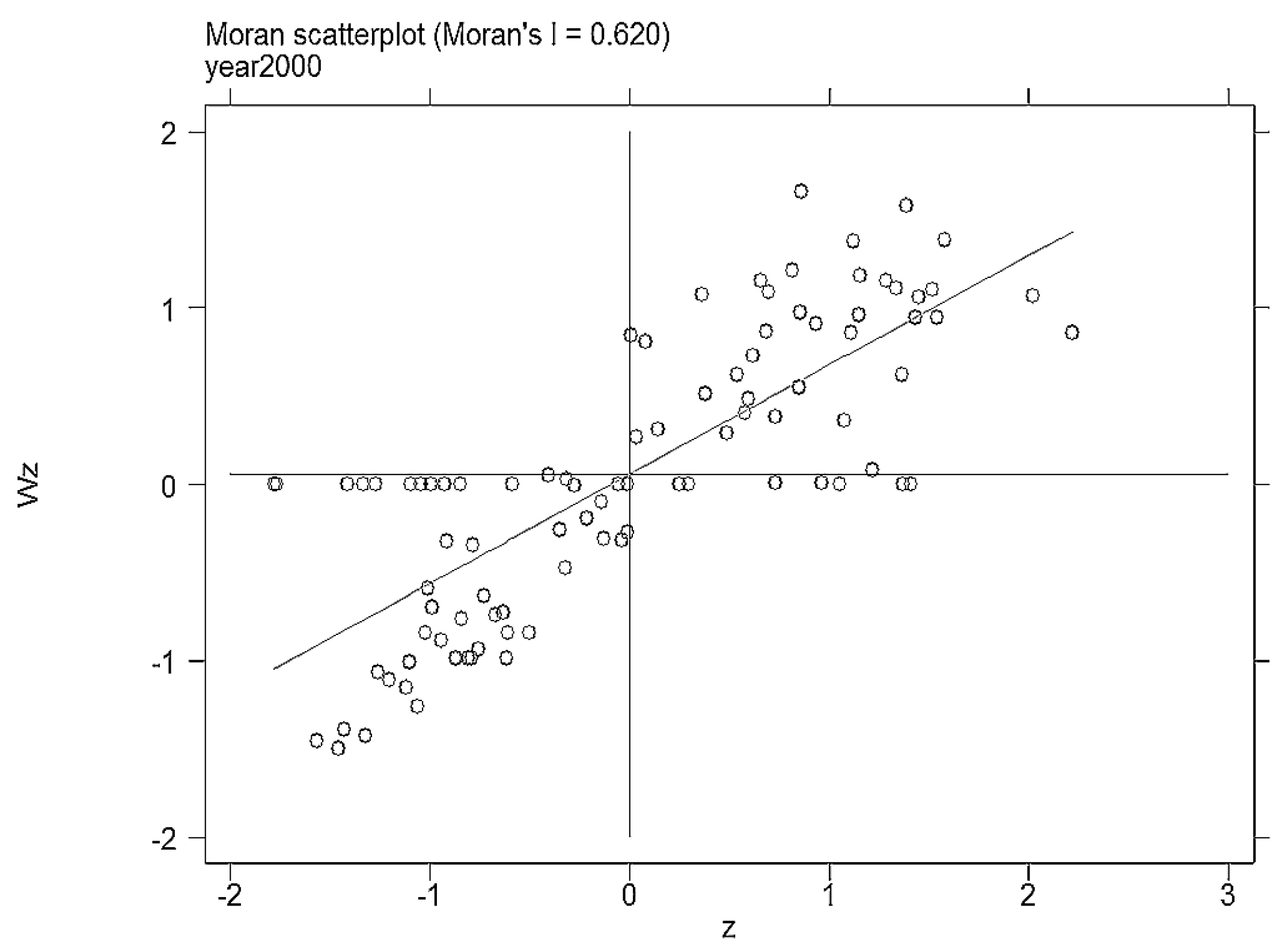
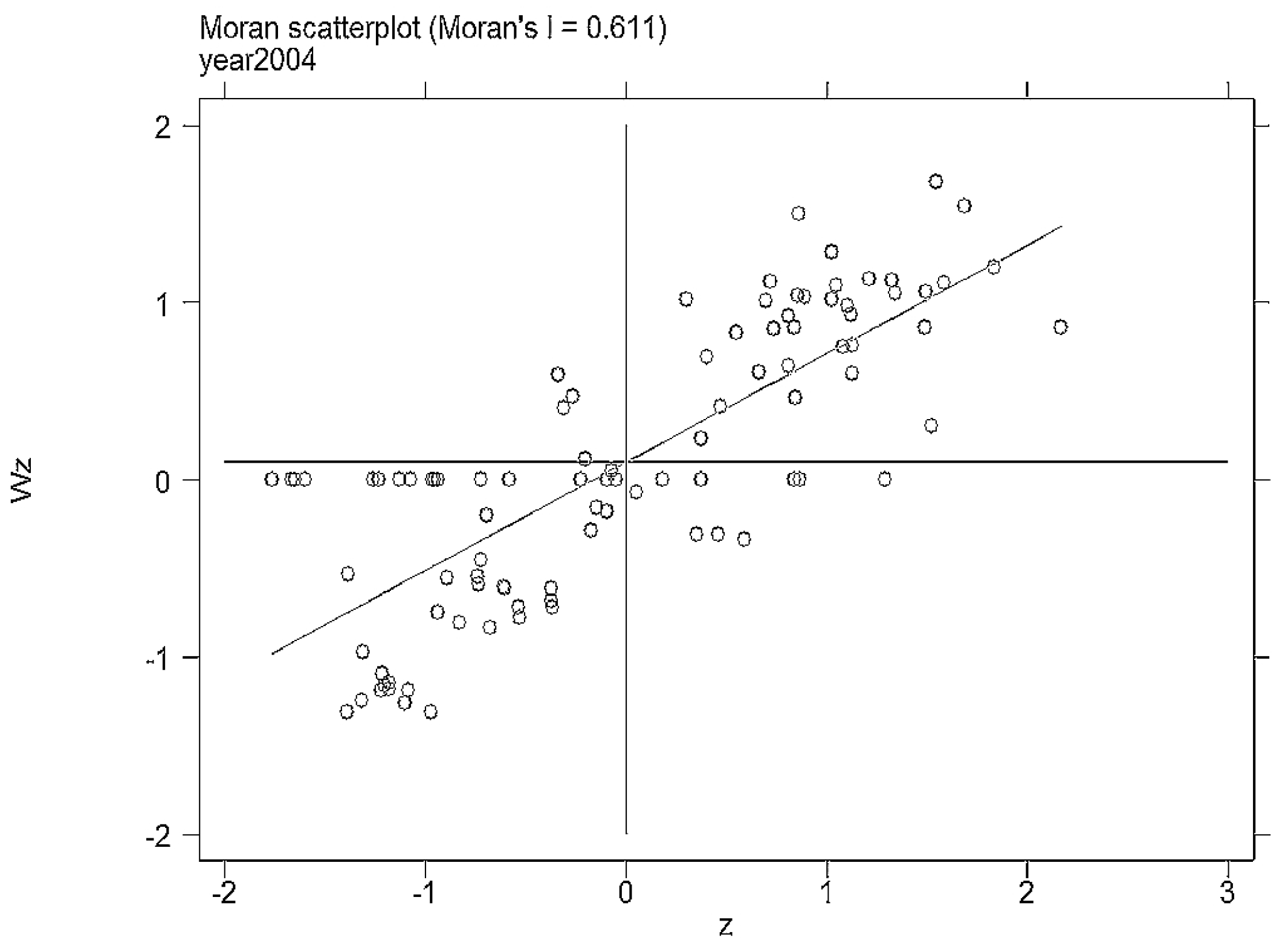
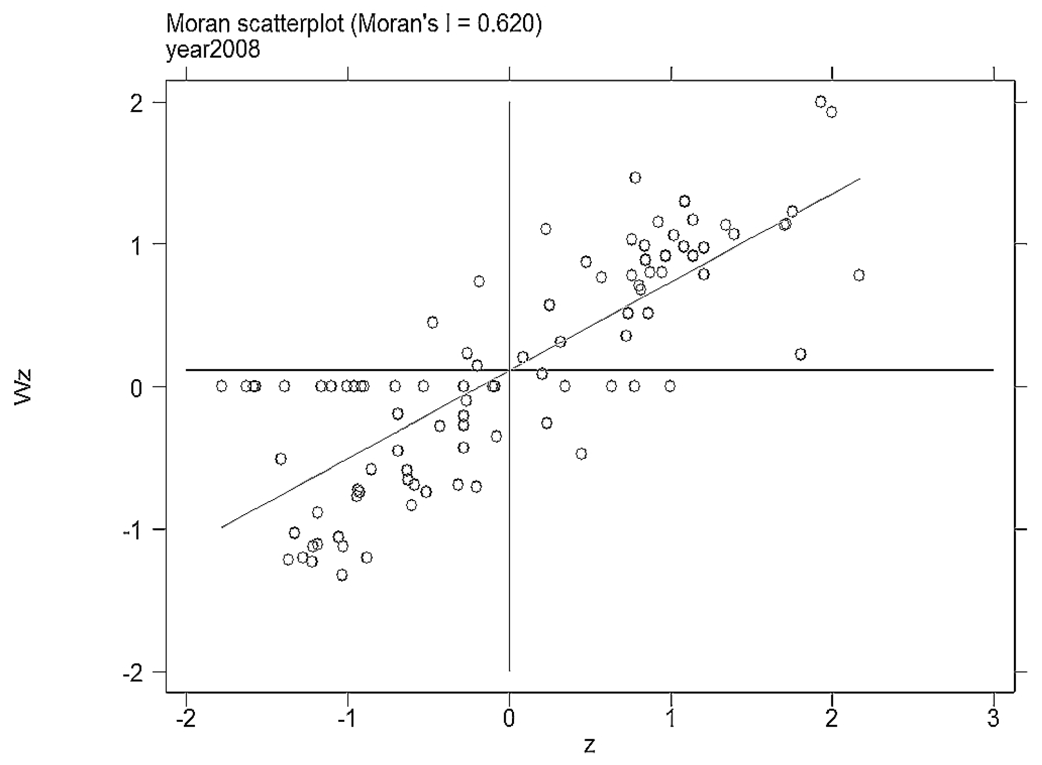
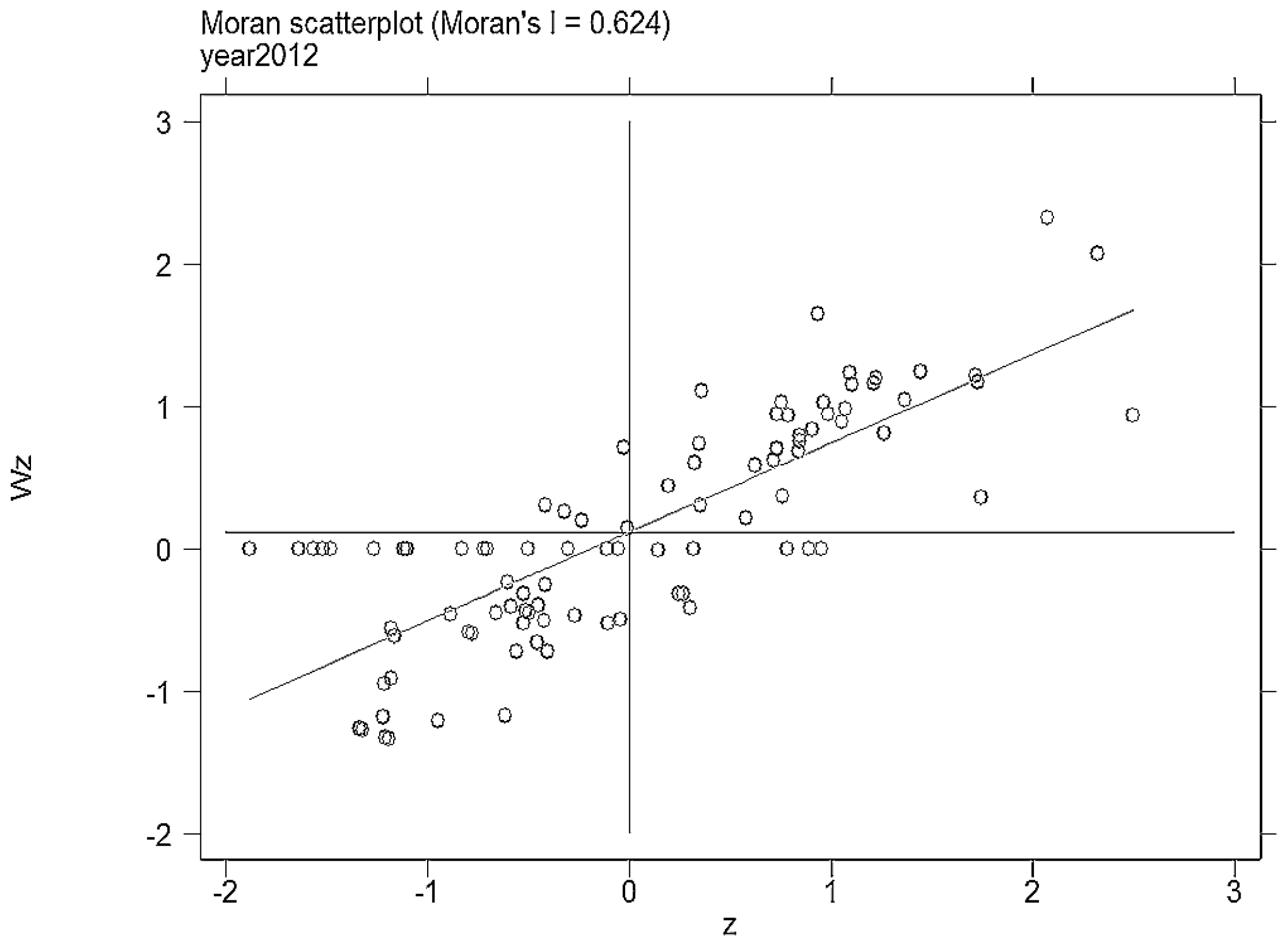
We further constructed the local Moran index based on the data of particulate matter emissions in China’s key cities from 2000 to 2012, to see whether there is a difference between the local Moran indices of different cities. Figure 1, Figure 2, Figure 3 and Figure 4 show the local Moran indices of key cities in 2000, 2004, 2008 and 2012, respectively (In fact, we have estimated the local moran indexes for each year from 2000 to 2012, which are not released here. If interested, please ask the author).
As shown in the figures, the local Moran indices of most cities fall in the first or third quadrants. This represents the existence of positive or negative correlations in the discharge of fine particulate matter in most cities. In the case of 2012, for example, there are only 11 cities displaying no spatial correlation. Through matching the relevant city serial number, there was an obvious correlation in eastern, central and western geographical space divisions.
According to the three economic zone division criteria proposed in “the National Economic and Social Development Seven Five-Year Plan” adopted by the National People’s Congress in 1985, we divided the sample of 95 cities into the eastern, central and western regions, and once again tested the convergence of fine particle emissions in different regions.
3.5. Spatial Convergence of PM 2.5
The regression results of the non-linear time-varying factor model of the sub-regional urban agglomeration are classified in Table 4. It can be seen that the three regions show a steady spatial convergence within regions. However, it should be noted that the convergence rate of PM 2.5 in the middle and west sub-regions, especially in the middle sub-region, are significantly higher than that in the east.
Through the sub-regional convergence test, we find that there exists an absolute time-converge of PM 2.5 emissions in 95 sample cities from 2000 to 2012. There has been a growing trend in the PM 2.5 emissions of China. Further, through the spatial converge test, we found that the convergence rates of PM 2.5 emissions in the middle and western regions are significantly higher than that of the eastern region. Since a large amount of previous research showed that China’s economic development had an obvious three-regional convergence situation [23,24,25], the further question is whether there is a different relation between the economic development and the pollution caused by the PM 2.5 emissions in different geographical regions in China. In the fourth section, we are prepared to test this problem.
4. Relationship between Regional Air Pollution and Economic Development
4.1. Test Model Construction of Environment Kuznets Curve
Our basic idea is to use the traditional Environmental Kuznets Curve (EKC) equation to investigate the existence of the EKC curve across the country as well as in different regions, and to further determine the shape of the curve. On the basis of this, in view of the possible spatial influence in different regions and the construction of the spatial panel for different regions, the existence of the EKC relationship hypothesis between PM 2.5 and the regional economic development is examined under the spatial effect.
Based on the idea above, we first construct the standard EKC test model shown in Equation (12):
where i is the number of the i-th city, and t is the corresponding year. is the estimated coefficient of the explained variable, is residual. refers to the average PM 2.5 concentration of city i in time t. refers to the per capita GDP of city i in the year of t, expressed in yuan. is the square of per capita GDP and refers to the cube of per capita GDP.
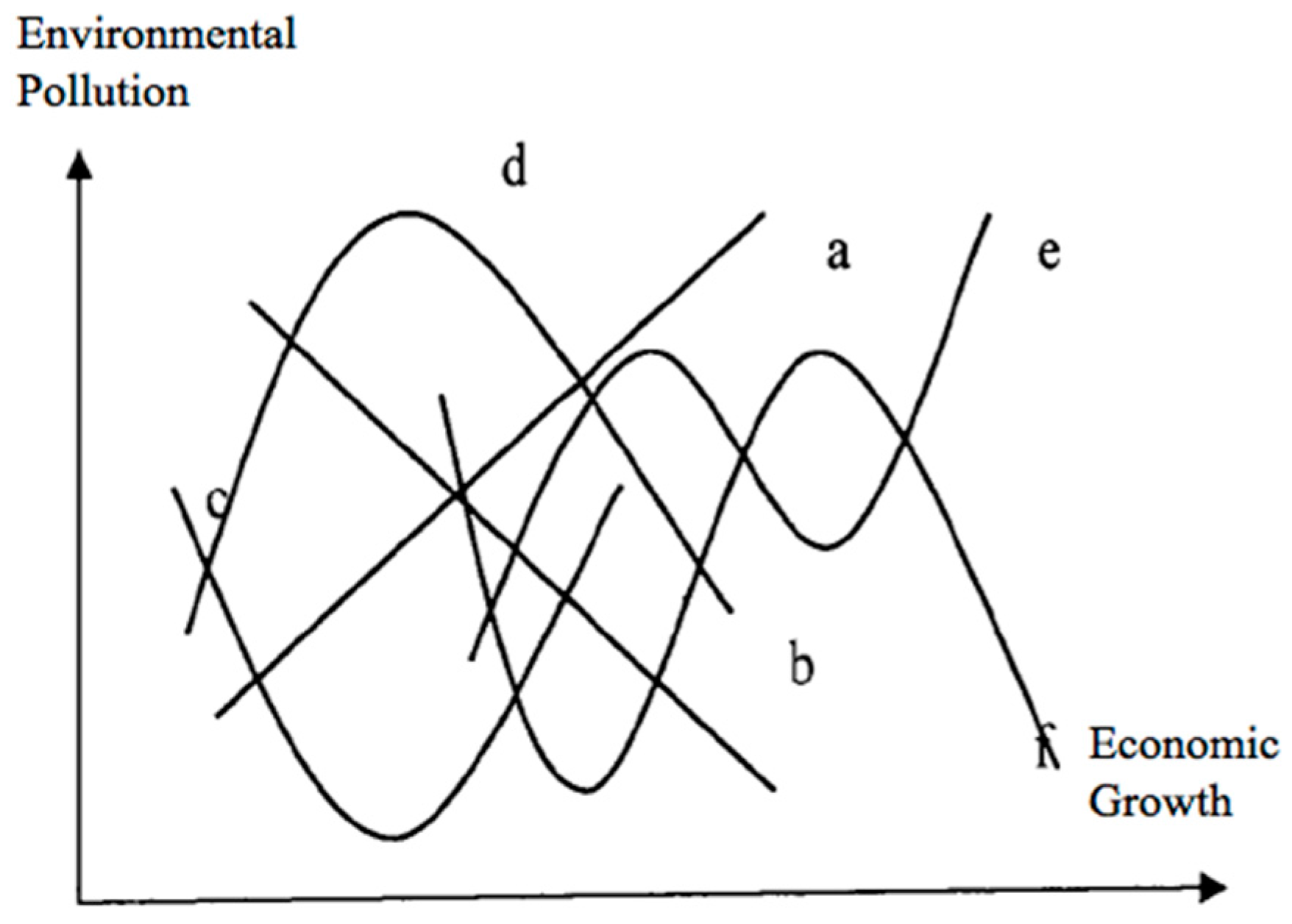
As in all EKC evaluation studies (e.g., Grossman G M, Krueger A B, 1992 [26]), Equation (12) includes the square per capita GDP and cube per capita GDP, with their coefficients and representing the solution of the first-order condition and the second-order condition, which help to evaluate the shape of ECK between pollution and economic development [26]. Different shape of EKC could be found from Figure 5, and the decision rule could be shown as follows:
- (1)
- when , and , , it indicates that environmental pollution becomes more serious with economic growth, as shown in straight line a in the following graph;
- (2)
- when , and , , it indicates that environmental pollution is improved with economic growth, as shown by straight line b;
- (3)
- when , and , , it indicates that the quality of the environment in the process of economic growth improves after deterioration, and there is a positive U-shaped relationship, as shown in curve c;
- (4)
- when , and , , it indicates that the quality of the environment in the process of economic growth deteriorates after improvement, there is an inverted U-shaped relationship, which conforms to the typical EKC hypothesis, as shown in curve d;
- (5)
- when , and , , it shows that environmental pollution has a positive N-type curve with the level of economic growth, that is, with economic growth, environmental pollution increases first and then decreases, and then increases again, as shown by curve e;
- (6)
- when , and , , it shows that there is an inverted N-type curve between environmental pollution and the level of economic growth, as shown by curve f;
- (7)
- when , and , , it suggests that there is no environmental EKC curve.
After completing the judgment of the common panel model, we further construct the spatial lag model, and the relationship between the PM 2.5 emissions and the regional economic development is further tested. Since the spatial lag model assumes that the dependent variable depends on the weighted average effects of the spatial adjacent unit variables, we construct the following equation:
where PM 2.5 refers to the dependent variable, X refers to independent variable, W is spatial autoregressive coefficient and ε is expressed as random error terms.
According to the spatial error effect model (SEM), in the setting process of the model, it is likely that some variables related to the explanatory variables will be omitted, and these variables have spatial autocorrelation. At the same time, there may be random error shock space spillover effect among regions. The equation is expressed as:
where refers to error of spatial autocorrelation.
4.2. Test Results
Table 5 shows the results of the correlation between PM 2.5 emissions and regional economic development in the urban sample of the whole cities, and sub-regional urban samples shown by panel regression.
According to the EKC judgment rules from the previous section, we can see from the table that there is a positive N-type EKC curve between the economic growth and PM 2.5 emissions of the whole sample. The same result also exists in the middle sub-region. The other test results show that, except for an inverted E-type EKC curve in the eastern region under a fixed effect model test, other test results do not support the hypothesis that correlation between economic growth and PM 2.5 emissions conformed to EKC in the eastern and western regions of China.
However, recent studies on geographic data panel analysis have shown that spatial lag effect and spatial error effect in spatial regional data may also have an effect on panel regression results. Therefore, we attempt to construct the spatial lag effect model (SLM) and the spatial error effect model (SEM) to try to further verify the relationship between economic growth and PM 2.5 emissions in the three regions of China from the perspective of the spatial panel. Before the construction of the relevant models, we consider what kind of spatial model should be tested.
In general, the spatial model study applied SLM or SEM based on the comparison of SLM model and SLM-LM and SEM-LM, as well as SLM-Robust and SEM-Robust. If SLM-LM is more significant than SEM-LM, and SLM-Robust passes the significant test while SEM-Robust does not, SLM will be selected. In the case of the contrary, SEM will be selected. In this study, our test results are shown in Table 6.
From the results of spatial lag and spatial error models, there are both spatial lag effect and spatial error effects in the sub-zone sample group. In this paper, we again carried out model tests of spatial lag effect and spatial error effect on the three regions, the results of which are shown in Table 7.
It can be seen from the results that, after considering spatial lag effect and spatial error effect, in the east, middle and west zones divided by study sample, there is a significant positive N-type EKC curve relationship between PM 2.5 emissions and regional economy. This indicates that during the observed period, China’s regional PM 2.5 emissions increased first, then declined, and then increased again with the development of the economy. The results of this test are also in accordance with the fact that Chinese residents had more significant physical reactions to haze pollution brought by PM 2.5 after the year of 2012.
5. Policy Recommendations
Based on the above analysis of air pollution and economic growth, we can get the following revelation on future sustainable governance policy for northeast Asia region and for China. First of all, in northeast Asian countries, resources and environmental issues have become an important factor affecting the economic growth. To some extent, they have even become the bottleneck of a country’s economic growth. The conclusion of this paper also shows that haze pollution emissions represented by PM 2.5 keep growing throughout China. Similar to all industrialized countries, China’s haze pollution problems are accompanied by industrialization. Environmental problems caused by industrial production are becoming more and more prominent, and the constraints of resources and the environment are becoming increasingly significant. Therefore, whether it is for the use of resource products or air pollution control, we should proceed from the overall situation paying attention to pollution control policy and the top design of resource utilization policy, and strengthening the consistency of policy implementation throughout the nation.
Secondly, although this paper mainly focused on the haze pollution issue inside China, as the first section introduced, haze is a boundary environmental pollution. Considering that most northeast Asian countries are border connected, the more haze pollution China faces, the more potential pollution risk there will be for its neighboring countries. Hence, all of northeast Asia should face such challenges together, and have more interaction through their governments and industries in order to bring out more concerted actions in the future.
Thirdly, economic development is an important driving force for industrial environmental efficiency convergence. China’s environmental efficiency and its cities’ respective levels of economic development, urban scale, financial capacity, and industrial development characteristics are often highly consistent. From 2000 to 2012, the phenomenon that PM 2.5 emissions increased first and then declined and further increased again with the development of the economy occurred in the east, middle and west regions of China. The selected cities, which again warned that the relationship between the economy and the environment does not necessarily follow a transformation path where the environmental quality improves, then deteriorates and further improves again with the economic growth, as assumed in traditional economic theory. In real world, due to the changes in economic structure and industrial structure, the environmental quality in the region is likely to have many inflection points with the change of the size of an economy.
Therefore, China’s future economic development mode must be transformed from quantity to quality to avoid the inhibition effect of China’s rising industrial development capacity to the convergence of environmental efficiency, especially for the middle and western sub-regions. As the main carriers to undertake the industrial transfer in the eastern developed areas, the middle and western sub-regions are regarded as the key areas of the development of future industrialization, urbanization, low-carbon industry and green transformation in China. Therefore, we need to start from the beginning to: reinforce the policy guidance of clean industrial production, energy saving, a recycling economy, and other aspects; strengthen the support to capital, technology and personnel of resource conservation and environmental protection; encourage the elimination of backward technology and enhance environmental control to reduce environmental pollution and improve industrial environmental efficiency.
Finally, there are significant differences in the environmental efficiency of industries in the different regions of China, as well as the possible spillover of environmental regulation policies’ impact and the diffusion of environmental pollution. In view of this, in the formulation of environmental governance policies, regional coordinated development policies and differentiated measures should be formulated on a case-by-case basis for spatial differences among regions. More importantly, such coordination should be taken into account more for geographically close cities or urban agglomerations. On this basis, it is possible to realize a win–win situation of economic growth and environmental protection by considering the conflict between the development policies of each administrative region and promoting the formation of a good environment cooperation mechanism across regions to gain a sustainable future.
6. Research Conclusions
This study used satellite telemetry data, the non-linear time-varying factor model, and the global and local Moran indices to test the spatial-time convergence of PM 2.5 in China. The results showed that there is an absolute convergence of PM 2.5 emissions in China in time trend, and there is a difference in the convergence rates of the eastern, central and western regions of China. This difference is manifested in the central and western regions, especially in the central region. The convergence rate in the central region of PM 2.5 is significantly higher than that of eastern region.
Furthermore, the results of the general panel model and the spatial analysis model reveal that the relationship between economic development and air pollution is still different in all regions of the country. First, there is a positive N-type EKC curve between economic growth and PM 2.5 emissions in selected sample cities. Secondly, considering spatial lag effect and spatial error effect, the regression model of the Environmental Kuznets Curve shows that there is also a significant positive N-type EKC curve relation between economic growth and PM 2.5 emissions in the east, middle and west sub-regions of China.
Acknowledgments
This research was funded by the China Social Science Fund (fund number 15CJL048. I would like to thank panel members from SAC 2017 for their delightful suggestions and comments on an early version of this paper. I would also like to thank anonymous reviewers for their comments on all drafts of this paper. Special thanks goes to Xu Xu for her help of all the grammar check. All remaining errors are mine.
Conflicts of Interest
The author declares that they have no conflict of interest.
References
- Song, M.; Wang, S.; Cen, L. Comprehensive efficiency evaluation of coal enterprises from production and pollution treatment process. J. Clean. Prod. 2015, 104, 374–379. [Google Scholar] [CrossRef]
- Song, M.; Zheng, W. Computational analysis of thermoelectric enterprises’ environmental efficiency and Bayesian estimation of influence factors. Soc. Sci. J. 2016, 53, 88–99. [Google Scholar] [CrossRef]
- Huang, B.; Meng, L. Convergence of per capita carbon dioxide emissions in urban China: A spatio-temporal perspective. Appl. Geogr. 2013, 40, 21–29. [Google Scholar] [CrossRef]
- Zhang, Y.-J.; Liu, Z.; Zhang, H.; Tan, T.-D. The impact of economic growth, industrial structure and urbanization on carbon emission intensity in China. Nat. Hazards 2014, 73, 579–595. [Google Scholar] [CrossRef]
- Tietenberg, T.; Lewis, L. Environmental & Natural Resources Economics: International Edition; Pearson Education: London, UK, 2011. [Google Scholar]
- Chameides, W.L.; Lindsay, R.W.; Richardson, J.; Kiang, C.S. The role of biogenic hydrocarbons in urban photochemical smog: Atlanta as a case study. Science 1988, 241, 1473–1476. [Google Scholar] [CrossRef] [PubMed]
- Rupasingha, A.; Goetz, S.J.; Debertin, D.L.; Pagoulatos, A. The environmental Kuznets curve for US counties: A spatial econometric analysis with extensions. Pap. Reg. Sci. 2004, 83, 407–424. [Google Scholar] [CrossRef]
- Englert, N. Fine particles and human health—A review of epidemiological studies. Toxicol. Lett. 2004, 149, 235. [Google Scholar] [CrossRef] [PubMed]
- Engel-Cox, J.A.; Hoff, R.M. Qualitative and quantitative evaluation of MODIS satellite sensor data for regional and urban scale air quality. Atmos. Environ. 2004, 38, 2495–2509. [Google Scholar] [CrossRef]
- Peters, A. Particulate matter and heart disease: Evidence from epidemiological studies. Toxicol. Appl. Pharmacol. 2005, 207 (Suppl. S2), 477. [Google Scholar] [CrossRef] [PubMed]
- Strazicich, M.C.; List, J.A. Are CO2 Emission Levels Converging Among Industrial Countries? Environ. Res. Econ. 2003, 24, 263–271. [Google Scholar] [CrossRef]
- Camarero, M.; Picazo-Tadeo, A.J.; Tamarit, C. Are the determinants of CO2 emissions converging among OECD countries? Econ. Lett. 2013, 118, 159–162. [Google Scholar] [CrossRef]
- List, J.A. Have Air Pollutant Emissions Converged among U.S. Regions? Evidence from Unit Root Tests. South. Econ. J. 1999, 66, 144–155. [Google Scholar] [CrossRef]
- Bulte, E.; List, J.A.; Strazicich, M.C. Regulatory Federalism and the Distribution of air Pollutant Emissions. J. Reg. Sci. 2007, 47, 155–178. [Google Scholar] [CrossRef]
- Phillips, P.C.B.; Sul, D. Transition Modeling and Econometric Convergence Tests. Econometrica 2007, 75, 1771–1855. [Google Scholar] [CrossRef]
- Donkelaar, A.V.; Martin, R.V.; Brauer, M.; Kahn, R.; Levy, R.; Verduzco, C.; Villeneuve, P.J. Global Estimates of Ambient Fine Particulate Matter Concentrations from Satellite-Based Aerosol Optical Depth: Development and Application. Environ. Health Perspect. 2010, 118, 847–855. [Google Scholar] [CrossRef] [PubMed]
- Van Donkelaar, A.; Martin, R.V.; Brauer, M.; Boys, B.L. Global Annual PM 2.5 Grids from MODIS, MISR and SeaWiFS Aerosol Optical Depth (AOD), 1998–2012; NASA Socioeconomic Data and Applications Center (SEDAC): Palisades, NY, USA, 2015. [Google Scholar]
- Van Donkelaar, A.; Martin, R.V.; Brauer, M.; Boys, B.L. Use of Satellite Observations for Long-term Exposure Assessment of Global Concentrations of Fine Particulate Matter. Environ. Health Perspect. 2015, 123, 135–143. [Google Scholar] [CrossRef] [PubMed]
- Environmental Protection Ministry of the People’s Republic of China. China Environmental Quality Report 2013; China Environmental Press: Beijing, China, 2014.
- Tobler, W.R.A. Computer Movie Simulating Urban Growth in the Detroit Region. Econ. Geogr. 2016, 46, 234–240. [Google Scholar] [CrossRef]
- Austin, E.; Coull, B.; Thomas, D.; Koutrakis, P. A framework for identifying distinct multipollutant profiles in air pollution data. Environ. Int. 2012, 45, 112–121. [Google Scholar] [CrossRef] [PubMed]
- Anselin, L. Local Indicators of Spatial Association—LISA. Geogr. Anal. 1995, 27, 93–115. [Google Scholar] [CrossRef]
- Lin, Y.; Liu, M. China’s Economic Growth Convergence and Income Distribution. World Econ. 2003, 8, 33–39. [Google Scholar]
- Peng, G. Convergence of Clubs in China’s Regional Economy. J. Quant. Tech. Econ. 2008, 12, 49–57. [Google Scholar]
- Shen, K.; Ma, J. The Characteristics of “Club Convergence” and Its Causes in China’s Economic Growth. Econ. Res. 2002, 1, 33–39. [Google Scholar]
- Grossman, G.M.; Krueger, A.B. Environmental Impacts of a North American Free Trade Agreement. Soc. Sci. Electr. Publ. 1992, 8, 223–250. [Google Scholar]
Figure 1.
The local Moran index in 2000.

Figure 2.
The local Moran index in 2004.

Figure 3.
The local Moran index in 2008.

Figure 4.
The local Moran index in 2012.

Figure 5.
The shape of the Environmental Kuznets Curve (EKC).


Table 1.
City names.
| Province | City | Province | City | Province | City | Province | City |
|---|---|---|---|---|---|---|---|
| Beijing | Beijing | Zhejiang | Hangzhou | Guangdong | Guangzhou | Hubei | Wuhan |
| Tianjin | Tianjin | Ningbo | Shenzhen | Yichang | |||
| Hebei | Shijiazhuang | Wenzhou | Zhuhai | Xiangyang | |||
| Tangshan | Jiaxing | Shantou | Hunan | Changsha | |||
| Qinghuangdao | Huzhou | Foshan | Zhuzhou | ||||
| Handan | Shaoxing | Jiangmen | Changde | ||||
| Baoding | Jinhua | Kanjiang | Inner Mongolia | Hohhot | |||
| Cangzhou | Quzhou | Huizhou | Baotou | ||||
| Langfang | Zhoushan | Dongguan | Guangxi | Nanning | |||
| Liaoning | Shenyang | Fujian | Fuzhou | Zhongshan | Liuzhou | ||
| Dalian | Xiamen | Hainan | Haikou | Guilin | |||
| Anshan | Putian | Sanya | Sichuan | Chengdu | |||
| Shanghai | Shanghai | Quanzhou | Shanxi | Taiyuan | Mianyang | ||
| Jiangsu | Nanjing | Zhangzhou | Jilin | Changchun | Yunnan | Kunming | |
| Wuxi | Longyan | Jilin | Shannxi | Xi’an | |||
| Xuzhou | Shandong | Jinan | Heilongjiang | Harbin | Baoji | ||
| Changzhou | Qingdao | Daqing | Gansu | Lanzhou | |||
| Suzhou | Zibo | Anhui | Hefei | Qinghai | Xining | ||
| Nantong | Dongying | Wuhu | Ningxia | Yinchuan | |||
| Lianyungang | Yantai | Maanshan | Xinjiang | Urumqi | |||
| Huai’an | Weifang | Jiangxi | Nanchang | ||||
| Yanchen | Jining | Henan | Zhenzhou | ||||
| Yanzhou | Weihai | Luoyang | |||||
| Zhenjiang | Linyi | Anyang | |||||
| Chongqing | Chongqing | Guizhou | Guiyang | Nanyang | |||
Table 2.
Study on convergence and robustness of whole city samples.
| L(t) = log(t + 1) | L(t) = log(t) | L(t) = log(t − 1) | |
|---|---|---|---|
| b | 18.41003 | 18.40986 | 18.40966 |
| 2.83 | 2.83 | 2.83 | |
| a | −52.02939 | −52.02884 | −52.02823 |
| −2.88 | −2.88 | −2.88 |
Data under each coefficient is standard deviation.
Table 3.
The global Moran index.
| Year | Moran Index | E(I) | sd(I) | p-Value |
|---|---|---|---|---|
| 2000 | 0.768 | −0.011 | 0.102 | 0.000 |
| 2001 | 0.749 | −0.011 | 0.102 | 0.000 |
| 2002 | 0.786 | −0.011 | 0.102 | 0.000 |
| 2003 | 0.806 | −0.011 | 0.102 | 0.000 |
| 2004 | 0.786 | −0.011 | 0.102 | 0.000 |
| 2005 | 0.764 | −0.011 | 0.102 | 0.000 |
| 2006 | 0.769 | −0.011 | 0.102 | 0.000 |
| 2007 | 0.761 | −0.011 | 0.102 | 0.000 |
| 2008 | 0.777 | −0.011 | 0.102 | 0.000 |
| 2009 | 0.817 | −0.011 | 0.102 | 0.000 |
| 2010 | 0.840 | −0.011 | 0.102 | 0.000 |
| 2011 | 0.820 | −0.011 | 0.102 | 0.000 |
| 2012 | 0.764 | −0.011 | 0.102 | 0.000 |
Table 4.
Sub-regional convergence test and robustness study.
| Region | Parameter | L(t) = log(t + 1) | L(t) = log(t) | L(t) = log(t − 1) |
|---|---|---|---|---|
| East | b | 1.434791 | 1.434617 | 1.434422 |
| 0.22 | 0.22 | 0.22 | ||
| a | −4.860393 | −4.859842 | −4.859232 | |
| −0.26 | −0.26 | −0.26 | ||
| Middle | b | 79.61884 | 79.61868 | 79.61949 |
| 4.78 | 4.78 | 4.78 | ||
| a | −222.0877 | −222.0872 | −222.0866 | |
| −4.79 | −4.79 | −4.79 | ||
| West | b | 71.89226 | 71.89209 | 71.8919 |
| 12.09 | 12.09 | 12.09 | ||
| a | −200.5981 | −200.5975 | −200.5969 | |
| −12.13 | −12.13 | −12.13 |
Data under each coefficient is standard deviation.
Table 5.
Panel estimation of the sub-regional Environmental Kuznets Curve.
| 95 Cities | East | |||||
|---|---|---|---|---|---|---|
| GLS | Random | Fixed | GLS | Random | Fixed | |
| C | 37.95818 *** | 37.95818 *** | 42.02255 *** | 42.80357 *** | 42.80357 *** | 60.3849 *** |
| 2.393372 | 1.314376 | 1.60851 | 4.629631 | 2.752783 | 3.326338 | |
| GDP | 0.0003144 *** | 0.0003144 *** | 0.0001439 | 0.0002078 | 0.0002078 | −0.000649 *** |
| 0.0000671 | 0.0000548 | 0.0000662 | 0.0001927 | 0.0001743 | 0.0001933 | |
| GDP2 | −1.26 × 10⁻⁹ *** | −1.26 × 10⁻⁹ * | −1.75 × 10⁻¹⁰ | −9.70 × 10⁻¹⁰ | −9.70 × 10⁻¹⁰ | 7.96 × 10⁻⁹ *** |
| 4.16 × 10⁻¹⁰ | 4.70 × 10⁻¹⁰ | 5.15 × 10⁻¹⁰ | 2.42 × 10⁻⁹ | 2.81 × 10⁻⁹ | 2.89 × 10⁻⁹ | |
| GDP3 | 1.64 × 10⁻¹⁵ ** | 1.64 × 10⁻¹⁵ * | −9.55 × 10⁻¹⁷ | 1.06 × 10⁻¹⁵ | 1.06 × 10⁻¹⁵ | −2.76 × 10⁻¹⁴ ** |
| 6.58 × 10⁻¹⁶ | 9.04 × 10⁻¹⁶ | 9.57 × 10⁻¹⁶ | 8.87 × 10⁻¹⁵ | 1.23 × 10⁻¹⁴ | 1.23 × 10⁻¹⁴ | |
| R2 | 0.0268 | 0.0268 | 0.0289 | 0.0062 | 0.0062 | 0.0174 |
| Hausman | 19.39 *** | 71.17 *** | ||||
| Middle | West | |||||
| GLS | Random | Fixed | GLS | Random | Fixed | |
| C | 35.87851 *** | 35.87851 *** | 36.41891 *** | 30.89278 *** | 30.89278 *** | 45.63498 *** |
| 1.381159 | 2.349397 | 2.601868 | 2.132795 | 5.16157 | 6.787467 | |
| GDP | 0.0005855 *** | 0.0005855 *** | 0.0005685 *** | 0.0001557 | 0.0001557 | −0.0010218 |
| 0.0000509 | 0.0000883 | 0.0000974 | 0.0003291 | 0.0006236 | 0.0007374 | |
| GDP2 | −2.90 × 10⁻⁹ *** | −2.90 × 10⁻⁹ *** | −2.85 × 10⁻⁹ *** | 1.89 × 10⁻⁹ | 1.89 × 10⁻⁹ | 2.37 × 10⁻⁸ |
| 3.72 × 10⁻¹⁰ | 6.27 × 10⁻¹⁰ | 6.67 × 10⁻¹⁰ | 1.10 × 10⁻⁸ | 2.05 × 10⁻⁸ | 2.30 × 10⁻⁸ | |
| GDP3 | 4.05 × 10⁻¹⁵ *** | 4.05 × 10⁻¹⁵ *** | 4.01 × 10⁻¹⁵ *** | −4.79 × 10⁻¹⁴ | −4.79 × 10⁻¹⁴ | −1.82 × 10⁻¹³ |
| 6.58 × 10⁻¹⁶ | 1.09 × 10⁻¹⁵ | 1.15 × 10⁻¹⁵ | 9.77 × 10⁻¹⁴ | 1.90 × 10⁻¹³ | 2.07 × 10⁻¹³ | |
| R2 | 0.1932 | 0.1932 | 0.1933 | 0.0077 | 0.0077 | 0.0164 |
| Hausman | 0.19 | 8.99 *** | ||||
*, **, *** respectively represented the results were significant at the level of 10%, 5% and 1%, data under each coefficient is standard deviation.
Table 6.
Test results of the Spatial Lag Effect (SLM) and Spatial Error Effect (SEM) Models.
| East | Middle | West | ||||
|---|---|---|---|---|---|---|
| Result | p-Value | Result | p-Value | Result | p-Value | |
| LM Test for Spatial Lag | 342.16 | 0.0000 | 21.1906 | 0.0000 | 20.393 | 0.0000 |
| Robust | 8.7567 | 0.0031 | 12.3319 | 0.0004 | 4.3701 | 0.0366 |
| LM Test for Spatial Error | 335.5374 | 0.0000 | 17.9619 | 0.0000 | 17.8563 | 0.0000 |
| Robust | 2.1337 | 0.1441 | 9.1032 | 0.0026 | 1.8334 | 0.1757 |
Table 7.
Results of Spatial Lag Effect and Spatial Error Effect.
| East | Middle | West | ||||
|---|---|---|---|---|---|---|
| SLM | SEM | SLM | SEM | SLM | SEM | |
| GDP | 1.251658 *** | 0.921818 *** | 0.00049175 *** | 0.000430432 *** | 0.001485549 *** | 0.001329185 *** |
| 22.55061 | 25.39407 | 12.232792 | 13.861633 | 8.427643 | 8.507777 | |
| GDP2 | −1.28 × 10⁻² *** | −9.36 × 10⁻³ *** | −1.90 × 10⁻⁹ *** | −1.78 × 10⁻⁹ *** | −3.54 × 10⁻⁸ *** | −3.13 × 10⁻⁸ *** |
| −14.1 | −16.2 | −6.86 | −8.75 | −6.04 | −6.07 | |
| GDP3 | 4.10 × 10⁻⁵ *** | 3.10 × 10⁻⁵ *** | 2.45 × 10⁻¹⁵ *** | 2.35 × 10⁻¹⁵ *** | 2.60 × 10⁻¹³ *** | 2.30 × 10⁻¹³ *** |
| 10.154337 | 12.4 | 5.34 | 7.06 | −3.65 | 4.73 | |
| R2 | 0.8983 | 0.9552 | 0.896 | 0.9344 | 0.9119 | 0.9346 |
| w | −0.236068 *** | −0.236068 *** | −0.236068 *** | |||
| e | 0.55599 *** | 0.334969 *** | 0.332994 *** | |||
*, **, *** respectively represented the results were significant at the level of 10%, 5% and 1%, data under each coefficient is standard deviation.
© 2017 by the author. Licensee MDPI, Basel, Switzerland. This article is an open access article distributed under the terms and conditions of the Creative Commons Attribution (CC BY) license (http://creativecommons.org/licenses/by/4.0/).
Share and Cite
MDPI and ACS Style
Pu, Z. Time-Spatial Convergence of Air Pollution and Regional Economic Growth in China. Sustainability 2017, 9, 1284. https://doi.org/10.3390/su9071284
AMA Style
Pu Z. Time-Spatial Convergence of Air Pollution and Regional Economic Growth in China. Sustainability. 2017; 9(7):1284. https://doi.org/10.3390/su9071284
Chicago/Turabian StylePu, Zhengning. 2017. "Time-Spatial Convergence of Air Pollution and Regional Economic Growth in China" Sustainability 9, no. 7: 1284. https://doi.org/10.3390/su9071284
Note that from the first issue of 2016, this journal uses article numbers instead of page numbers. See further details here.