Article

Parameter Estimation of the Farquhar—von Caemmerer—Berry Biochemical Model from Photosynthetic Carbon Dioxide Response Curves

1
Wye Research and Education Center, University of Maryland, Queenstown, MD 21658, USA
2
APEC Climate Center, 12 Centum 7-ro, Haeundae-gu, Busan 48058, Korea
3
USDA-ARS Crop Systems and Global Change Lab, Beltsville, MD 20705, USA
4
Department of Geographical Sciences, University of Maryland, College Park, MD 20742, USA
*
Author to whom correspondence should be addressed.
Sustainability 2017, 9(7), 1288; https://doi.org/10.3390/su9071288
Submission received: 26 April 2017 / Revised: 15 July 2017 / Accepted: 19 July 2017 / Published: 24 July 2017

Abstract

:
The Farquhar—von Caemmerer—Berry (FvCB) biochemical model of photosynthesis, commonly used to estimate CO2 assimilation at various spatial scales from leaf to global, has been used to assess the impacts of climate change on crop and ecosystem productivities. However, it is widely known that the parameters in the FvCB model are difficult to accurately estimate. The objective of this study was to assess the methods of Sharkey et al. and Gu et al., which are often used to estimate the parameters of the FvCB model. We generated An/Ci datasets with different data accuracies, numbers of data points, and data point distributions. The results showed that neither method accurately estimated the parameters; however, Gu et al.’s approach provided slightly better estimates. Using Gu et al.’s approach and datasets with measurement errors and the same accuracy as a typical open gas exchange system (i.e., Li-6400), the majority of the estimated parameters—Vcmax (maximal Rubisco carboxylation rate), Kco (effective Michaelis-Menten coefficient for CO2), gm (internal (mesophyll) conductance to CO2 transport) and Γ* (chloroplastic CO2 photocompensation point)—were underestimated, while the majority of Rd (day respiration) and α (the non-returned fraction of the glycolate carbon recycled in the photorespiratory cycle) were overestimated. The distributions of Tp (the rate of triose phosphate export from the chloroplast) were evenly dispersed around the 1:1 line using both approaches. This study revealed that a high accuracy of leaf gas exchange measurements and sufficient data points are required to correctly estimate the parameters for the biochemical model. The accurate estimation of these parameters can contribute to the enhancement of food security under climate change through accurate predictions of crop and ecosystem productivities. A further study is recommended to address the question of how the measurement accuracies can be improved.

1. Introduction

The FvCB leaf photosynthesis model for C3 plants [1,2] is fundamental for the prediction of leaf responses to environmental variation [3]. This model has been widely used to simulate CO2 assimilation and the response of plants to climate change for different spatiotemporal scales [4,5,6,7,8,9,10,11], due to its solid theoretical basis and simplicity [12]. It is also frequently used in reverse to quantify the underlying biochemical properties (i.e., the model parameters) of leaves under different environmental conditions [13,14,15,16,17]. These parameters are often considered easier to estimate from gas exchange measurements rather than making the required in vitro measurements to quantify enzyme activity. This is because it is difficult to extract functional enzymes from many species [18], and in vitro conditions seldom represent those experienced in vivo [19]. According to the different versions of FvCB model [1,20,21,22,23], up to 8 parameters (Vcmax, Kco, J, Tp, α, gi, Rd, and Γ*) can be estimated from an analysis of the response of the net assimilation rate (An) to intercellular CO2 concentration (Ci) if enough accurate data points are available [2].
There are numerous publications discussing the different parameterization methods associated with An/Ci curves [2,12,24,25,26,27,28,29]. Each method relies on different assumptions and has technical limitations. Most approaches assume that α = 0 and that the Kco and Γ* can be chosen a priori from estimates in previous studies to determinate Vcmax, Jmax, Tp, Rd and gm [2,12,22,26,27]. Gu et al. [2] extended the method of Ethier and Livingston [12] to propose an exhaustive dual optimization (EDO) approach to estimate the parameters from fitting An/Ci curves. All of the curve-fitting methods minimize an objective function; e.g., the sum of the square of errors (SSE), based on the nonlinear FvCB model, with a limited number of measurements (typically 8–12, [2,24,26,30]) and the expected accuracy of a measured An/Ci curve (see [2,25,26] for comprehensive reviews). Depending on the equations used for fitting the parameters, two major groups of methods can be distinguished: Group I directly fits parameters with the FvCB model [14,25,26,27,31] and Group II fits parameters with a quadratic equation [2,12]. The implementation is sensitive to the methods used. The estimated parameters can be substantially different when using different An/Ci curve-fitting methods on the same dataset [2,25,26,29]. It is frequently difficult to determine which method is superior based on the measures of SSE because of the characteristics of the FvCB model [2], the assumption that the assigned values of the kinetic properties of Rubisco are the correct ones, and the number of parameters to be estimated [24].
Some studies compared different fitting methods to determine the parameters of the FvCB model. Miao et al. [26] made a comparison of six different methods using 160 randomly selected An/Ci datasets from 4 shrubby indicator species, including highbush blueberry (Vaccinium corymbosum L.), dangleberry (Gaylusaccia frondosa L.), coastal fetterbush (Eubotrys racemosa L.) and sweet pepperbush (Clethra alnifolia L.). They concluded that the method developed by Sharkey et al. [27] was among the ‘best’, based on the lowest minimum of the root mean square error. Gu et al. [2] stated that their approach could estimate reliable FvCB parameters using error-free synthetic An/Ci curves and predicted limited states that matched chlorophyll fluorescence patterns from actual datasets.
An erroneous determination of the FvCB model parameters can lead to inaccurate predictions of ecosystem productivity, because the potential errors can worsen when moving to larger temporal and spatial scales (e.g., from field measurements over short periods to ecosystem predictions over long periods) [32,33]. However, to the best of our knowledge, there is little information on a comprehensive test of these different fitting methods using common generated datasets superimposed by possible measurement errors. The objective for this study was to assess the two approaches for fitting the FvCB model: group I (Sharkey et al.’s method) and group II (Gu et al.’s method).

2. Materials and Methods

2.1. The FvCB Model and Characteristics

An/Ci curves are fitted with the FvCB model for C3 leaves [1] that accounts for gm and whereby An is given as
A n = m i n { W c , W j , W p } ( 1 Γ * C c ) R d ,   for   C c > ( 1 + 3 α ) Γ *
A n = m i n { W c , W j , W p } ( 1 Γ * C c ) R d ,   for   C c > ( 1 + 3 α ) Γ * ,
A n = m i n { W c , W j } ( 1 Γ * C c ) R d ,   for   Γ * C c ( 1 + 3 α ) Γ * ,
A n = W c ( 1 Γ * C c ) R d ,   for   C c < Γ * ,
W c = V c m a x C c C c + K c o ,
W j = J C c 4 C c + 8 Γ * ,
where min{} denotes ‘the minimum of’.
α in Equation (6) is often set to zero, and Equation (6) can be then reduced to
W p = 3 T p C c C c Γ * ,   f o r   C c > Γ * .
In the above equations, Wc, Wj and Wp are the carboxylation rates limited by Rubisco (Ac state), the Ribulose 1,5-bisphosphate (RuBP) regeneration (Aj state) and triose phosphate utilization (TPU) (Ap state), respectively; Equation (3) is one of the points where the Aj state is equal to the An state (see next the section for an explanation); Cc is the chloroplastic CO2 partial pressure and can be estimated by
C c = C i A n g m .
A typical condition for assessing An/Ci curves at saturating light levels is to assume that J approaches Jmax, the maximum rate of electron transport. If light is not saturating at the time of measurement, Jmax must be calculated from J [24]. In this study, we assume that Jmax = J.
Combining Equations (1)–(8), the relationship between An and Ci in the Ac, Aj and Ap states can be expressed as three segment hyperbolic curves [2,12], respectively;
{ A n c 2 g m C i c A n c + p c A n c + q c C i c + u c = 0 , A n j 2 g m C i j A n j + p j A n j + q j C i j + u j = 0 , A n p 2 g m C i p A n p + p p A n p + q p C i p + u p = 0 ,
where the subscripts c, j and p refer to the Ac, Aj and Ap states, respectively; gm, p, q and u are 4 ‘coefficients’ in each segment of an An/Ci curve. The general form of Equation (9) is
A n 2 g m C i A n + p A n + q C i + u = 0
In the Ac state,
{ g m = g m ,   p c = [ ( V c m a x R d ) + g m K c o ] , q c = ( V c m a x R d   ) g m ,   u c = [ V c m a x Γ * + K c o R d ] g m .  
In the Aj state,
{ g m = g m ,   p j = [ ( J m a x 4 R d ) + 2 Γ * g m ] , q j = ( J m a x 4 R d   ) g m ,   u j = ( J m a x 4 + 2 R d ) Γ * g m .  
In the Ap state,
{ g m = g m ,   p p = [ ( 3 T p R d ) ( 1 + 3 α ) Γ * g m ] , q p = ( 3 T p R d   ) g m ,   u p = [ 3 T p ( 1 + 3 α ) R d ] Γ * g m .  
When α = 0 , Equation (9) in the Ap state is reduced to
A p   = 3 T p R d
Mathematically, there are two positive roots for the quadratic Equation (10),
A n = g m C i p ± ( g m C i p ) 2 4 ( u 4 q C i ) 2 ,
but only one root meets the constraints of the FvCB model.
A n = g m C i p ( g m C i p ) 2 4 u + 4 q C i 2 .
The above equation describes An as a function, Ci [12]. Equation (16) consists of up to three segments (states). The three states share one common coefficient gm, while the other coefficients (p, q and u) are combinations of the common parameters gm, Γ* and Rd and the state specific parameters Vcmax and Kco in the Ac state, Jmax in the Aj state, and Tp and α in the Ap state.

2.2. Data Generation

2.2.1. Constraints for the Parameters

To generate datasets in order to test the methods, the following constraints for the parameters are required. All parameters are greater than zero to keep their biological meanings. The FvCB model is a monotonic increasing function in both Ac and Aj states and a monotonically decreasing function when α > 0, or it is a constant in the Ap state when α = 0. The three states follow a fixed order along the Ci axis [2].
If an An/Cc curve consists of both Ac and Aj states, there could, mathematically, be two conditions: (1) The two states could be exactly the same if Jmax/4 = Vcmax and Kco = 2Γ*. Since Kco > 2Γ* [2,22], however, the two states cannot be the same. (2) There are two intersection points where Anc = Anj. The first point is at Cc = Γ*; Anj < Anc when Cc < Γ*. We define An = Anc when Cc < Γ* to create the fixed order of Ac and Aj states (Equation (3)). The second point is defined as the transition point Ccc_cj by combining Equations (4) and (5),
C c c _ c j = J m a x 4 V c m a x 2 Γ * / K c o 4 V c m a x J m a x .
Since 2Γ*/Kco < 1, the constraints for Vcmax and Jmax can be expressed as:
4 V c m a x > J m a x .
When Aj and Ap states coexist, the constraint for Jmax as a function of Tp is [2]:
J m a x > 12 T p .
When Ac and Ap states coexist, the constraint for Vcmax as a function of Tp is
V c m a x > 3 T p .
When three states coexist, the constrains are given by
{ V c m a x ,   J m a x , T p , K c o ,   Γ * , R d ,   g m , α > 0 , K c o > 2 Γ * ,   C c ( 1 + 3 α ) Γ * ,   in   A p   state ,   A n = A n c   when   C c Γ * ,   4 V c m a x > J m a x > 12 T p .  

2.2.2. Criteria for Deriving Parameters

An involved parameter is a parameter that is presented in the given dataset. A non-resolvable parameter is defined as an involved parameter whose value cannot be correctly derived. It should be noted that resolvable, non-resolvable, and noninvolved parameters were defined by Gu et al. [2]. More detailed information on these definitions can be found in Gu et al. [2]. The equality of an estimated parameter against its “true value” is defined by an equivalency at the accuracy of three decimal places if the lowest precision of the An/Ci dataset is three or higher, or at the lowest precision of the An/Ci dataset if the precision of An/Ci is less than three decimal places. Since there are limitations due to measurement accuracy, the number of data points of the An/Ci dataset, and the fitting methods used, an estimated parameter might be equal to its “true value” by chance. To stop this result from biasing our analysis, a correctly estimated parameter is defined here as one that is obtained only if all resolvable parameters in this dataset are equal to their “true values”. If the numbers of data points in Ac, Aj and Ap states are x, y and z, respectively, the data point distribution is written as (x, y, z). More detailed information on the theoretical resolvability of parameters can be found in Gu et al. [2].
In practice, all of the measurements are subject to measurement errors (Appendix A). Therefore, the measured points lie near to, but not on, the theoretical curve. A number of techniques are needed to obtain the optimal approximation of the “true value”. The common methods for estimating the parameters of the FvCB model are based on the minimization of an objective function which characterizes a goodness-of-fit of a particular curve with respect to the given set of data points. For example, the parameters are estimated by minimizing the SSE [2,29]:
f   = i = 1 n c ( A c i A c m i ) 2 + j = 1 n j ( A j j A j m j ) 2 + k = 1 n p ( A p k A p m k ) 2 ,
where Aci, Ajj and Apk are the calculated net assimilation rates at point i in the Ac, Aj, Ap states respectively; Acmi, Ajmj and Apmk are the measured counterparts, respectively; and subscripts nc, nj and np are the numbers of counterpart points, respectively. The objective equation used in the methods of Sharkey et al. and Gu et al. are similar to Equation (22); however, the calculation procedures are different.

2.2.3. Generation of Datasets

The parameters were randomly chosen from selected parameter ranges with three decimal places. Vmax varied from 20.000 to 160.000 μmol m−2 s−1, Jmax from 20.000 to 250.000 μmol m−2 s−1, Tp from 5.000 to 15.500 μmol m−2 s−1, Rd from 0.010 to 5.000 μmol m−2 s−1, gm from 0.100 to 30.000 μmol m−2 s−1 Pa−1, Γ* from 0.100 to 5.000 Pa, Kco from 20.000 to 100.000 Pa, and α from 0.001 to 1.000. As a special case, α = 0, with the requirement of the constraints mentioned in the previous section (Equation (21)). Ci ranges from 5 to 150 Pa in both cases. We assumed that the datasets were collected at a leaf temperature of 25 °C and an air pressure of 100 Pa. Each set of parameters (except for α) was used to generate datasets with either α = 0 or α > 0. There were 200 datasets within each accuracy level, of which 100 used α = 0 and 100 with α > 0.
There were three accuracy subgroups (high, normal, and varied). Firstly, a high accuracy implies the accuracy of the generated An and Ci to eight decimal places. Secondly, a normal accuracy dataset was defined as a dataset which is rounded off from a high accuracy dataset. Normal precision is the same as a typical open gas exchange system, e.g., Li-6400 (Li-Cor, Inc., Lincoln, NE, USA). In this case, An is rounded to three decimal places if An < 1.000 μmol m−2s−1, to two decimal places if 1.00 μmol s−1 m−1 < An < 10.00 μmol s−1 m−1, and to one decimal place if An > 10.0 μmol m−2 s−1; Ci is rounded to one decimal place if Ci < 100 μmol mol−1 and to an integer if Ci > 100 μmol mol−1. Datasets can commonly have measurement errors. The errors in An and Ci were calculated according to Equations (A5) and (A6), respectively, in the appendix. The precision of a dataset from the measurements is the same as a normal accuracy dataset. Varied accuracy datasets were generated without measurement errors, either with varied accuracy or varied data points. The parameters used to generate varied accuracy datasets were: Vcmax of 45.572 μmol m−2 s−1, Jmax of 111.315 μmol m−2 s−1, Tp of 7.871 μmol m−2 s−1, Rd of 1.381 μmol m−2 s−1, gm of 1.897 μmol m−2 s−1 Pa−1, Γ* of 4.396 Pa, Kco of 43.616 Pa, and α of 0.352. The maximum number of data points in each state was nine. There were two subgroups in this group:
(i)
Datasets with varied data points. The accuracy of this dataset was eight decimal places; and the numbers of data points were 4, 5, 6, 7, 8, 9, and 12. The varied data point dataset was used to evaluate the impact of the number of data points on parameterization. It should be noted that these datasets are included in the high accuracy dataset.
(ii)
Datasets with varied accuracy. These datasets were with either eight or 12 data points, and accuracies were from one to eight decimal places. The varied accuracy dataset was used to identify the impact of accuracy on parameterization.

2.3. Fitting Methods

2.3.1. Gu et al.’s Method

Gu et al. [2] developed a four-step method to estimate the parameters of the FvCB model.
(1)
The enumeration of all possible data point distributions of three states of a given dataset. The three limited states must follow a certain pattern along the Ci axis in an order dictated by the FvCB model. The minimum numbers of data points (3 or 0, 2 or 0, 3 or 0) and the number of data points higher than the number of parameters to be derived are required for resolvable parameters. Under these conditions, the resolvable parameters are defined as Gu et al.s resolvable parameters to differentiate them from resolvable parameters as a general case. Thus, the minimum numbers of data points (3, 2, 3) and a minimum number of nine observed data points are required for all eight parameters to be resolvable. We refer to these as Gu et al.s requirements for all eight resolvable parameters. If only one or two states are Gu et al.s resolvable states, the dataset is Gu et al.s partially resolvable dataset and the resolvable parameters are Gu et al.s partially resolvable parameters. If a state does not meet the minimum data point requirement of Gu et al., Gu et al.’s method forces the dataset to meet the requirements by moving data points from one state to another. If the number of observed data points is zero in the Ap state, α = 0 and Tp = (asymptote of An + Rd)/three.
(2)
Fitting the FvCB model to each limited state distribution separately. In this step, the transition points are never calculated and the carboxylation rates in different states are never compared. The An is calculated with the submodel of the limited state to which the data point is assigned.
(3)
Detection and correction of inadmissible fits. Gu et al., [2] defined “inadmissible fits” as cases where the limitation states of the points in the A/Ci curve have not consistently or correctly identified the derived parameters. This step is only used for a dataset that contains multiple limited states. If the calculated limited state distribution is the same as the assigned limited state distribution, then the fit is admissible; otherwise, the fit is inadmissible. If the fit is inadmissible, the fit will be corrected via a penalization strategy.
(4)
Section of best fit. The best fit for an observed set of data is the method that gives the smallest value for the minimized objective function. If the values of the minimized objective function are equal when comparing across different limited state distributions, the one with fewer parameters is selected.

2.3.2. Sharkey et al.’s Method

Sharkey et al.’s method requires an initial set of estimated parameter values to be assigned and iteratively improves this set. The algorithm starts with two initial transition values for Ac and Aj states and Aj and Ap states; it then changes the values until the objective function is minimized. Since the parameters Kco, α and Γ* are assigned a priori, a maximum of five parameters are estimated. The three states share common parameters—gm and Rd —with state specific parameters of Vcmax in the Ac state, Jmax in the Aj state, and Tp in the Ap state. Thus, the minimum data point distribution is (1, 1, 1) and the minimum number of points is five for all five parameters to be resolvable. If the data points are only distributed in one state or in two states, the minimum number of data points is three or four, respectively, for all involved parameters to be resolvable. It should be noted that, for the same dataset, the number of Gu et al.’s resolvable parameters is different from that of Sharkey et al.’s, and both are different from the resolvable parameters in the general case.

2.3.3. Parameter Calculations

The parameter estimations were conducted in May 2011 to March 2012. The generated datasets were uploaded to the website http://Leafweb.ornl.gov to estimate the parameters by Gu et al.’s method. The detailed procedures can be found on the website. The Excel spreadsheet-software created by Sharkey et al. [27] (An/Ci curve fitting utility version 1.1) was used to test Sharkey et al.’s method.

3. Results

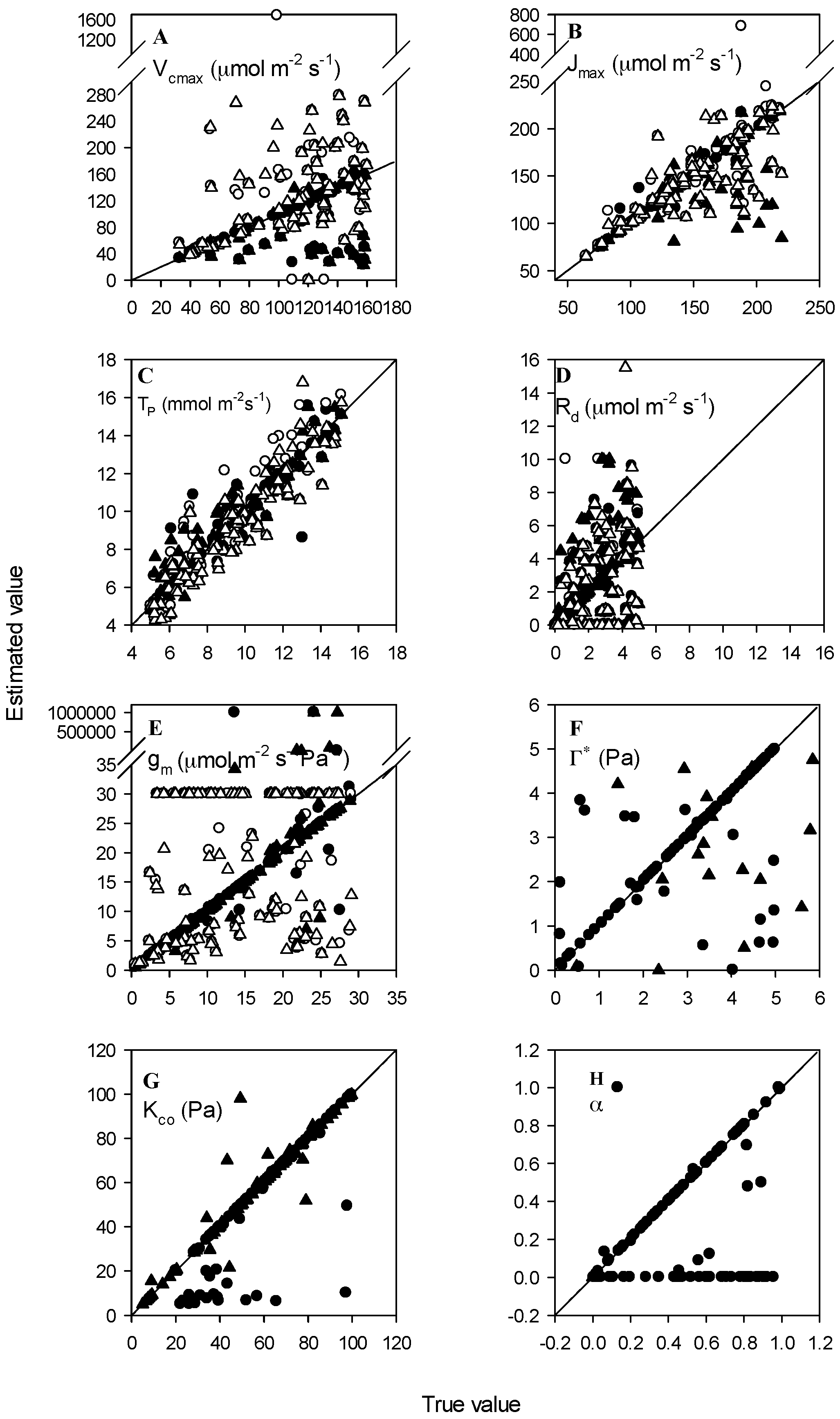
3.1. High Accuracy Dataset

Using Gu et al.’s method, all eight parameters were correctly retrieved in 23 datasets for high accuracy datasets with α > 0. In fact, there were a total of 33 datasets with all eight resolvable parameters, in which ten of the data sets did not meet the requirements set by Gu et al. for the minimum data point distribution (3, 2, 3) to retrieve all eight parameters. For datasets with α = 0, all eight parameters were correctly derived in 24 out of a total of 25 datasets that met the requirements of Gu et al. for all eight resolvable parameters. There was one exception, where a (3, 2, 10) dataset resulted in poor parameter estimation. These results imply that, when the dataset met Gu et al.’s requirements for all resolvable parameters in high accuracy datasets, Gu et al.s method obtained a full set of parameters for a dataset with α > 0, while the method might not correctly estimate all eight parameters for a dataset with α = 0.
For datasets with Gu et al.’s partially solvable parameters, the resolvable parameters may or may not be correctly estimated. For example, two datasets had the same data distribution (9, 0, 6). One dataset was able to correctly estimate all Gu et al.’s partially resolvable parameters, but another could not correctly estimate any parameter. Tp and α were non-involved parameters in this dataset, where the missing Ap state was incorrectly estimated because Tp was calculated by fitting the An/Ci curve with a sigmoid function and fixed α = 0. For example, one dataset (0, 15, 0) was identified as (5, 10, 0), and the non-involved parameters Vcmax, Kco, Tp and α were incorrectly derived.
For a dataset with one or two states which did not meet the minimum data point requirements set by Gu et al. for resolvable parameters, the specific parameters in this state could not be correctly estimated. For example, the method forced a dataset distribution of (7, 6, 2) to (7, 5, 3), leading to an incorrect estimation of all eight parameters.
The numbers of estimated parameters were larger than the resolvable parameters, which in turn were larger than the correctly estimated parameters. For example, for Vcmax, Jmax and Tp, when α > 0, the numbers of estimated parameters were 91, 74 and 100; the numbers of resolvable parameters were 71, 72 and 61; and the numbers of correctly estimated parameters were 52, 49, and 42, respectively (Table 1); when α = 0, the total numbers parameters were 86, 92 and 100 for estimated, 44, 62 and 45 for resolvable, and 37, 46 and 30 for correctly estimated parameters, respectively (Table 1). Obviously, gm was a resolvable parameter in any dataset, but could not always be correctly estimated.
Using Gu et al.’s method, more than half of the values of Vcmax, Kco, Jmax, gm, Tp and Γ* ranged within ±10% of error (Table 1). Some estimated values of gm could be very large; up to 100,000 μmol m−2 s−1 Pa−1 (Figure 1E). The estimated Rd values were more variable in comparison with other parameters, and many of the values were larger than the upper limit of 5.000 μmol m−2 s−1 used to generate datasets (Figure 1D). Most estimates of α were zero or very close to their “true values” when α > 0 (Figure 1H). The incorrectly estimated values of Vcmax, Kco, Jmax, Γ* and α showed a tendency to be underestimated, while Rd tended to be overestimated. About half of the incorrectly estimated gm values (except for extreme values) were overestimated, while Tp was evenly distributed around the 1:1 line (y = 1.002x, R2 = 0.941). The uneven distributions of the estimated parameters Vcmax, Kco, Γ*, Rd and α around the 1:1 line implied that the averages of these parameters may not be close to their “true values”.
Sharkey et al.’s method [27] was unable to correctly estimate any parameter for any dataset with both α = 0 and α > 0 (Table 1). All five unknown parameters—Vcmax, Jmax, gm, Tp and Rd—could be estimated for any dataset, and even for some noninvolved parameters in some datasets (Table 1), since Sharkey et al.’s method incorrectly forced data points into a missing state to minimize the objective function. Within ±10% of error ranges, the numbers for Vcmax, Jmax, gm, Tp and Rd were 22, 65, 41, 7 and 6, respectively, when α > 0, and were 23, 64, 63, 8, and 5 when α = 0, respectively. Vcmax and Jmax had extreme values in some datasets. Many values of gm reached their upper limit value of 30 μmol m−2 s−1 Pa−1. Overall, Vcmax, and gm were overestimated, about 40% of the Rd values were zero, Jmax was about evenly distributed around the 1:1 line (y = 1.016x, R2 = 0.462) with a few extreme large values, and Tp was about evenly distributed around the 1:1 line (y = 0.987x, R2 = 0.866) (Figure 1).

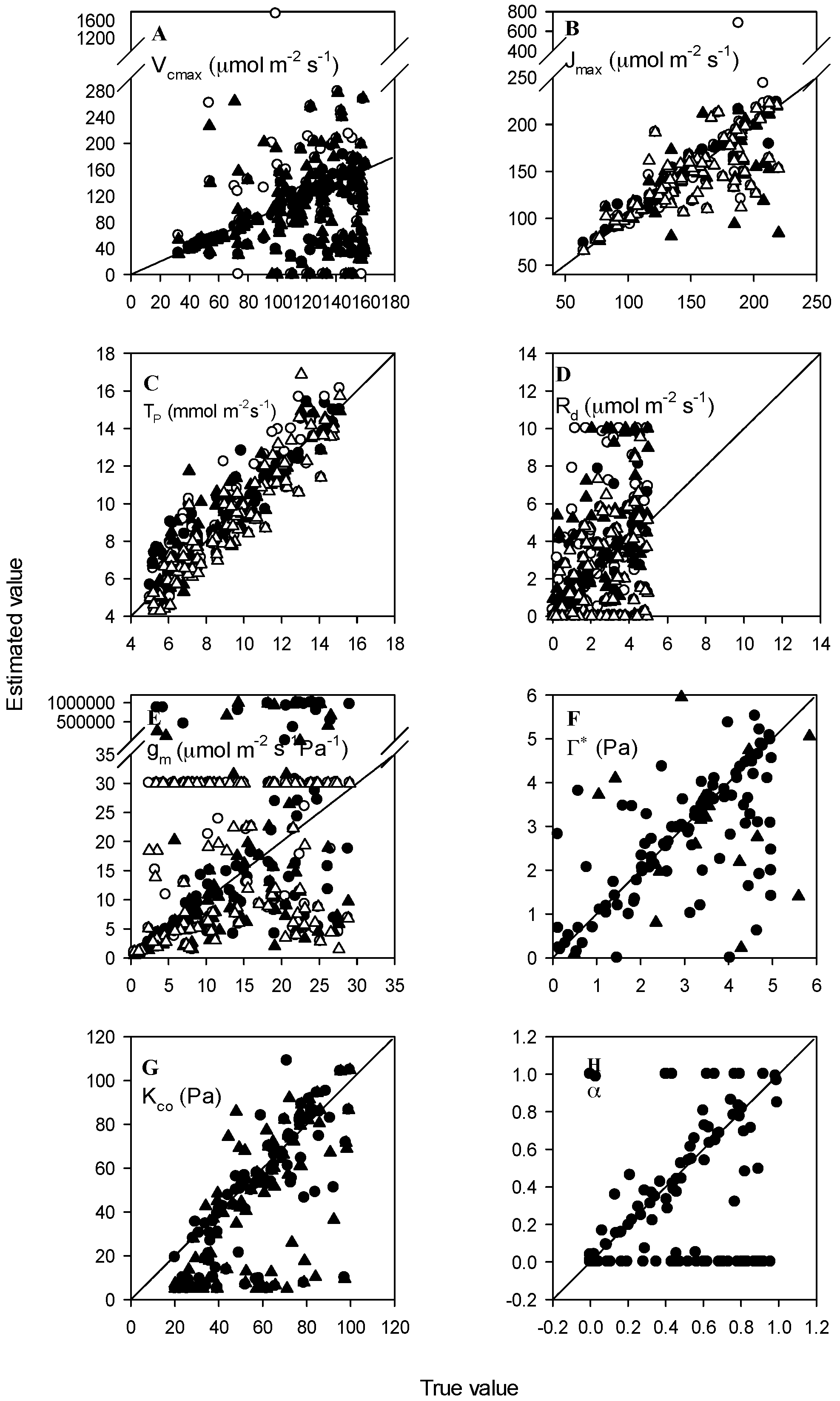
3.2. Normal Accuracy Datasets

For normal accuracy datasets with both α > 0 and α = 0, no parameters were correctly estimated using Gu et al.’s method. In comparison with the high accuracy dataset results, this suggests that the accuracy of An/Ci data was important for correctly determining the parameters. The total number of estimated parameters was more than the total number of resolvable parameters (except for gm) (Table 1). The number of estimated parameters was more than those utilizing high accuracy datasets, since more non-involved parameters were incorrectly estimated. Compared to the high accuracy datasets, more datasets with a missing state were incorrectly identified as datasets with all three states available by changing a missing state to an available one. For example, a dataset (3, 0, 12) was assigned to (4, 2, 9). The total number of values within ±10% of their “true values” for Vcmax, Kco, Jmax, Tp, gm, Rd, Γ* and α were 55, 40, 65, 70, 26, 16, 48 and 26 for α > 0; and were 43, 27, 64, 67, 20, 12, 42 and 99 for α = 0, respectively (Table 1). These numbers were fewer than the corresponding parameters in the high accuracy dataset. Overall, Vcmax, Kco, was underestimated, Rd was overestimated and gm was generally underestimated. In some cases, gm was overestimated when the estimated value was higher than 20 μmol m−2 s−1 Pa−1. Most of the estimated parameters Γ*, Jmax and Tp were evenly distributed around the 1:1 line (y = 0.952x and R2 = 0.531 for Jmax, y = 1.001x and R2 = 0.958 for Tp) (Figure 2).
Using Sharkey et al.’s method [27], there were no correct parameters for both α = 0 and α > 0 (Table 1). All five unknown parameters—Vcmax, Jmax, gm, Tp and Rd—were estimated for any dataset (Table 1) within ±10% of error. The values of Vcmax, Jmax, gm, Tp and Rd were 24, 70, 6, 57 and 6, respectively, when α > 0; and 22, 59, 8, 51, and 8, respectively, when α = 0. Vcmax and Jmax had extreme values in some datasets. Many values of gm reached their upper constrained value of 30 μmol m−2 s−1 Pa−1 for both α = 0 and α > 0. Overall, the parameters Vcmax and gm were underestimated, Jmax and Tp were evenly distributed around the 1:1 line (y = 0.991x and R2 = 0.572 for Jmax, y = 0.976x and R2 = 0.800 for Tp), and many values of Rd were over their upper limit of 5.000 μmol m−2 s−1 when generated (Figure 2).

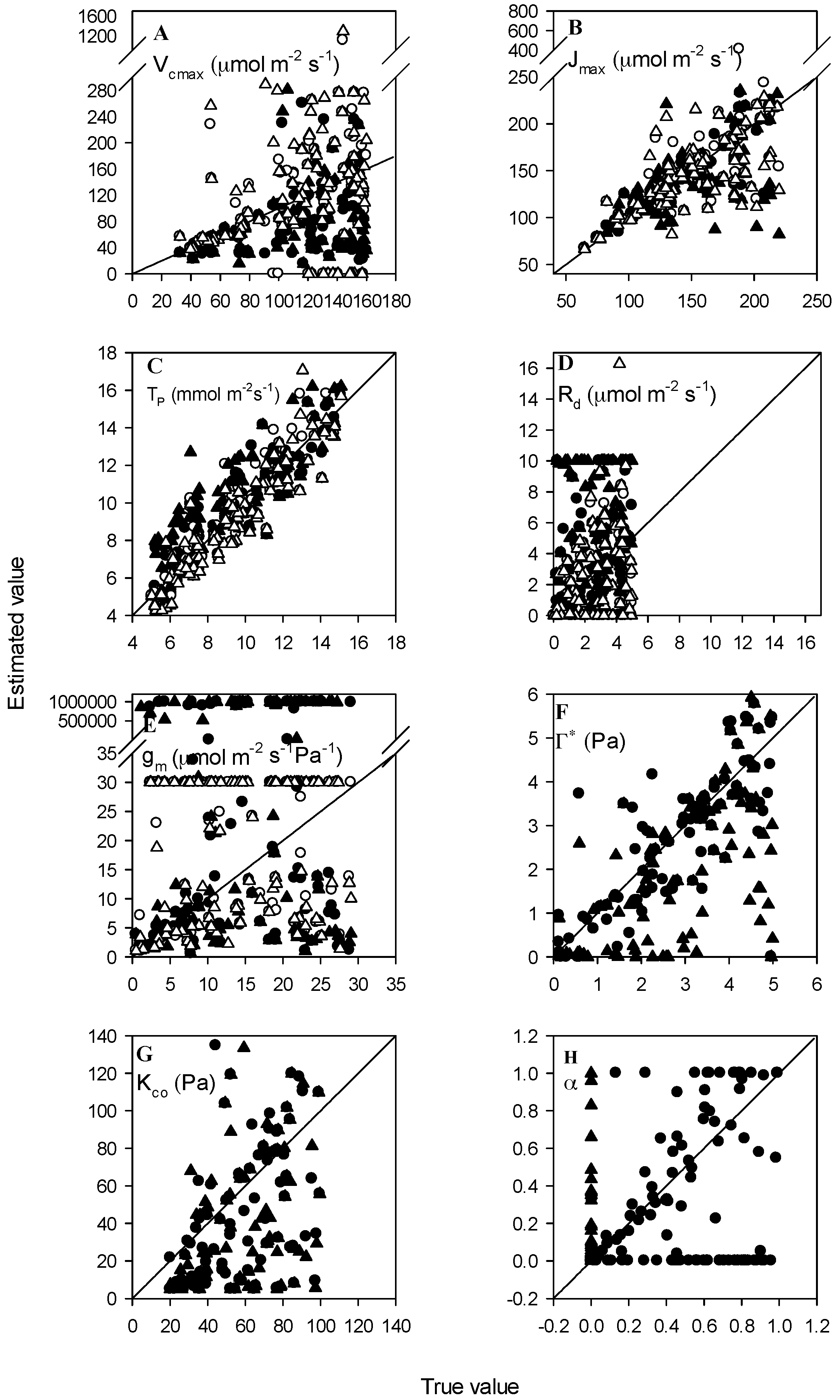
3.3. Datasets with Measurement Errors

Datasets with measurement errors are representative of observed data. Using Gu et al.’s method, the number of correctly estimated parameters was zero. The common parameters gm, Rd and Γ*, and the specific parameters Tp and α were estimated for all 100 datasets. The specific parameter Vcmax, Kco, or Jmax was estimated whenever its state was identified (Table 1). The number of estimated parameters was higher than that in normal accuracy datasets, indicating that more parameters would be estimated when using a less accurate dataset. The total numbers of values within ±10% of their “true values” for Vcmax, Kco, Jmax, Tp, gm, Rd, Γ* and α were 30, 10, 61, 64, 7, 7, 36 and 23 when α > 0; and 22, 7, 50, 51, 5, 8, 23 and 78 when α = 0, respectively (Table 1). The distributions of estimated parameters (except for Tp) were more scattered than that of normal accuracy datasets. Most of the values for Vcmax, Kco, gm and Γ* were underestimated (Figure 3A,G,E,F), while most of Rd and α were overestimated (Figure 3D,H). About half of the values of Tp and Jmax were overestimated.
Using Sharkey et al.’s method, there were no correctly estimated parameters for both α > 0 and α = 0 (Table 1). The numbers of parameters gm, Rd, Vcmax, Jmax, Tp, within ±10% errors were 8, 5, 24, 70 and 60 when α > 0, and 4, 7, 26, 61 and 63 when α = 0, respectively. There were similar numbers of estimated parameters within ±10% errors between datasets with measurement errors having α > 0 and α = 0 and for normal accuracy and measurement error datasets. This observation suggests that the impacts of the value of α and measurement errors on the estimated parameters were insignificant in datasets with large errors when using Sharkey et al.’s method. Overall, the distributions of the estimated parameters were similar to those of a normal accuracy dataset (Figure 3).

3.4. Datasets with Varied Data Points

Table 2 summarizes the results of the two methods using high accuracy datasets with a varied number of data points. Gu et al.’s method was unable to guarantee the correct estimation of any parameter values when the number of data points was eight or less. For datasets with nine and 12 points, all eight parameters could be correctly estimated if a dataset met the requirements set by Gu et al. for all eight resolvable parameters. However, the actual number of datasets with all eight resolvable parameters was much higher than the number of datasets that met the requirements of Gu et al. for all eight resolvable parameters. Gu et al.’s method could estimate the parameters gm, Rd, Γ*, Tp and α in any dataset (Table 2), though many of them were non-resolvable. Generally, the ratio of correctly estimated parameters to estimated parameters increased (except for Kco and Γ*) with an increasing number of observed data points for the An/Ci curve.
All parameters from the datasets were not correctly estimated by Sharkey et al.’s method (Table 2). The percentage of the number of estimated parameters with a ±10% error relative to the number of estimated parameters for Jmax and Tp ranged from about 33% when the number of data points was four. When the number of data points was 12 for gm, Rd and Γ*, this ranged from 0 to 20%. The estimated parameters were unevenly distributed around their “true values”.

3.5. Datasets with Varied Accuracy

Gu et al.’s method was unable to correctly estimate any parameter when the accuracy of datasets was four or fewer decimal places. For the datasets with decimal places 5, 6, 7 and 8, the numbers of datasets with correctly estimated parameters were 1, 4, 4, and 9 for datasets with eight data points, and 1, 9, 24 and 30 for datasets with 12 data points, respectively. If the number of data points was eight or fewer, there was no correct estimate for all eight parameters and no guarantee to correctly estimate any parameter. The numbers of datasets with a correctly estimated parameter increased with an increasing number of decimal places. For a dataset with 12 data points, it was possible to obtain all eight correct parameters when the accuracy was five or higher decimal places; however, to guarantee all eight parameters to be correctly estimated, a dataset must meet the requirements of Gu et al. for all eight resolvable parameters, and the accuracy must be seven or higher decimal places. In addition, in Gu et al.’s method, Vcmax was underestimated with an error of about 13–17% for datasets with eight data points and 11–15% for datasets with 12 data points. Jmax was slightly overestimated, with an error of about 0–7% for datasets with eight data points and 1–4% for datasets with 12 data points. Tp was overestimated, with an error of about 8–16% for for datasets with eight data points and 7–11% for for datasets with 12 data points. The estimated parameters gm, Kco Rd, α and Γ* had relatively large errors; for example, the errors of the mean values of Rd were from 80 to 243%.
Sharkey et al.’s method was unable to correctly estimate any parameter for datasets with varied accuracy. The estimated parameters did not change from their initial values when the accuracies of the datasets were five or more decimal places. Compared to the results using Gu et al.’s method, all the estimated parameters had less variation, as indicated by their smaller standard deviations (data not shown). The mean values of Vcmax were overestimated, with errors of 18% for datasets with eight data points, and 12–16% for datasets with 12 points. The mean values of Jmax were close to the “true value”, with errors of 5% for the datasets with eight data points, and 5–7% for datasets with 12 points. The means of Tp were overestimated with errors of 12–13% for datasets with eight data points, and 0–2% for datasets with with 12 points. Parameters gm and Rd had relatively large errors. The ranges of the relative changes of the mean gm and Rd were from 164 to 694%, and from −43 to 159%, respectively.

4. Discussion

Using high accuracy datasets, Gu et al.’s method was unable to correctly estimate the resolvable parameters that did not meet the requirements set by Gu et al. for resolvable parameters. This is because Gu et al.’s method forced these datasets to have the minimum number of data points as (0 or 3, 0 or 2, 0 or 3), which was an altered distribution. Gu et al.’s method could only correctly derive the resolvable parameters if the dataset satisfied the requirements of Gu et al. for resolvable parameters. However, since any observed dataset distribution is unknown and there are many fitted parameters, one cannot identify which set of parameters are correct.
Using normal accuracy datasets with measurement errors, Gu et al.’s and Sharkey et al.’s methods were unable to correctly estimate any parameter. As shown in Figure 1, Figure 2 and Figure 3, each set of estimated parameters from a high accuracy dataset, a normal accuracy dataset or a dataset with measurement errors were different. One of the main reasons for these differences was the accuracy of the datasets. Both methods were based on the standard nonlinear regression, which assumes that the error of An is a random variable whose population mean is zero and variance is constant, and that Ci is an independent variable without any error. Since only a few data points are available in each limited state, the sample error will vary considerably, simply by chance. A point with a larger error would tend to have a larger deviation from the curve and so would have a larger impact on the SSE. In contrast, a point with a smaller error would have a smaller influence. Minimizing the SSE would be inappropriate for datasets with a few data points with relative large errors.
The conditions for correctly estimating all eight parameters using Gu et al.’s method is a dataset with (1) a minimum of three data points for the limited state of Gu et al. for all resolvable parameters; (2) a minimum of nine data points for the An/Ci curve; (3) an accuracy of at least seven decimal places; and (4) α > 0. These requirements were necessary and sufficient conditions for Gu et al.’s method. If a dataset does not meet these conditions, Gu et al.’s method will be unable to guarantee a fit for any parameter. For example, in the dataset (2, 4, 2) with high accuracy, all the parameters were resolvable; however, Gu et al.’s method incorrectly identified it as (3, 5, 0), leading to all the parameters being incorrect (data not shown).
Sharkey et al.’s method (and other extant methods, see [26]) fits Vcmax, Jmax, Tp, Rd and gm simultaneously, using all the data points of an An/Ci curve, by fitting Equations (1)–(5) and (14), with fixed Kco and Γ*, and assuming α = 0. This approach simplifies the fitting method, but may introduce more errors to the estimated parameters if the wrong fixed values are used. Sharkey et al.’s method was unable to correctly estimate any parameters using all examined datasets. One of the major reasons for this could be the use of an incorrect value for the fixed parameters Kco, Γ*, and α. There are different Kco and Γ* values to choose from in the literature [12,27]. In addition, Kco changes across diverse species and environmental conditions. One can see from Equations (9)–(13) that a change in one or more parameters may lead to changes in all the other parameters; for example, if a dataset is only in the Ac state, by combining Equations (1), (4) and (8) and assuming independent of all involved parameters, one can have
V c m a x = ( C i + K c o ) g m A c ( C i Γ * ) g m A c ( A c + R d ) .
Thus, the direct impacts of Γ* and Kco on Vcmax are
V c m a x Γ * = ( C i + K c o ) g m A c [ ( C i Γ * ) g m A c ] 2 ( A c + R d ) g m ,
and
V c m a x K c o = ( A c + R d ) g m ( C i Γ * ) g m A c .
From the above equations, one can see that the direct effects of errors in Vcmax depend on the errors in Kco and Γ* and the values of Ac, Ci, gm and Rd. Thus, incorrect values for Kco and/or Γ* will inevitably lead to incorrect parameter estimates. This result is in agreement with that of Ethier and Livingston [12].
In Sharkey et al.’s methods, the CO2 partial pressure inside the chloroplast Ccs was estimated by (a similar estimation is also in the methods of Dubois et al. [24] and Miao et al. [26]):
C c s = C i A n m g m ,
where Anm is the measured net assimilation rate. Equation (26) is not identical to Equation (8); An in Equation (8) is the calculated value in the algorithm. Thus, a minimization of SSE based on Equation (26) or Equation (8) is different. The parameterization of a four-point curve in the Aj state (Table 3) illustrates this problem. The dataset with eight decimal places was generated using the same value of Γ* as in Sharkey et al.’s method to eliminate the effects of different values of Γ*. The two sets of estimated parameters were different from their “true values” and modeled Ajjs were slightly different from the ‘measured’ values. One can see that Sharkey et al.’s method was unable to correctly derive the parameters, even using a dataset with a high accuracy and the same fixed value as in the method.
Because the distribution of data points is unknown, it is possible for Sharkey et al.’s method to assign data points to the wrong states to minimize SSE, especially if a state is missing. Table 4 shows an example in which there was one dataset with 12 data points only in the Ac and Aj states. If the data points were assigned to the same states as when it was generated (I), the SSE was larger than if the last three data points were assigned to the Ap state, which was larger than if the transitional point between Ac and Aj was also adjusted. The estimated parameters were different among the three conditions (except for Rd and gm) and were different from their “true values.” It is worth noting that this is an intrinsic problem in Sharkey et al.’s method, because of the limited accuracy and number of data points of an An/Ci curve. It is very easy to miss a state, especially the Ap state [24]. This result can be explained by considering that the incorrect identification of the distribution of data points led to incorrect parameter estimation.
Both the methods of Sharkey et al. and Gu et al. have assigned constraints for some parameters based on prior knowledge; for example, gm ≤ 30 μmol m−2 s−1 Pa−1 in Sharkey et al.’s method, and Rd ≤ 10 μmol m−2 s−1, gm ≤ 1,000,000 μmol m−2 s−1 Pa−1, and Γ* ≥ 0 Pa in Gu et al.’s method. There were also different constraints found in other methods in the literature, such as the constraint of −3 < Rd < 50 μmol m−2 s−1 in Dubois et al. [24]. Firstly, if a parameter is estimated within the range of its constraint, the local minimum must be achieved in the range of the constraint. Secondly, the constraints are subjective choices which are probably not realistic; for example, we obtained Rd as zero by Sharkey et al.’s method (data not shown), and Γ* as zero (data not shown) by Gu et al.’s method. Thirdly, if a parameter is equal to its constraint, which is likely to be incorrect, this incorrect parameter may substantially affect the estimates of other parameters. The problems of finding a local minimum and non-uniqueness of the parameters is intrinsic to nonlinear regression; for example, in Sharkey et al.’s method, the estimates of the parameters were sensitive to the initial values (Table 3). There are similar problems in the method of Dubois et al. [24] and Miao et al. [26], as stated by Gu et al. [2].
However, the best fit but unreliable parameter set may be used to predict An from Ci if the SSE is small, as argued by Ethier and Livingston [12]. The four An/Ci curves modeled by the three sets of parameters with 15 data points (7, 6, 2) were compared. The three sets of parameters were high accuracy, including measurement errors, and derived from curves generated using the parameters fitted to the dataset with measurement errors by methods of Gu et al. and Sharkey et al., respectively. All curves are superposed.
The distributions of the estimated parameters (except for Tp) by both methods using a normal accuracy dataset and a dataset with measurement errors were very scattered. The majority of the estimated parameters were either overestimated or underestimated (Table 1, Figure 2 and Figure 3), implying that the mean values of these estimated parameters could not represent the “true values”. This can be explained by low data accuracies and by the intrinsic problems in both methods. The estimated Tp was evenly distributed around the 1:1 line, indicating that the mean Tp was close to its “true value”; this was because Tp is almost equal to A n 3 (Equations (1), (6), and (7)) since An >> Rd in the Ap state.

5. Conclusions

In this study, we tested Sharkey et al.’s [21] commonly-used An/Ci curve fitting method, and the method developed recently by Gu et al. [2], using datasets with a number of An/Ci curve points from four to 15 and accuracies from one to eight decimal places. The generated datasets were conservative. In the literature, the typical number of data points of an An/Ci curve is eight to 12, which is considered enough for estimation [2,24,26,30]. The accuracy of the measured data in a typical open gas exchange system is one decimal place; e.g., Li-6400. The error level of the generated datasets was lower than normally seen in practice, because only one source of measurement error, e.g., the random noise of CO2 ±0.2 μmol mol−1, was imposed as an error to the datasets; other error sources were not included [34].
To correctly estimate the parameters of an An/Ci curve, we have to consider data accuracy and the number and distribution of data points as well as error distribution. Based on the results using different generated datasets, we concluded that Sharkey et al.’s method failed to correctly estimate the parameters, while Gu et al.’s method was unable to correctly estimate the parameters using a dataset with a number of data points fewer than five or with an accuracy of four or fewer decimal places. At least eight data points were required for Gu et al.’s method to correctly estimate all eight parameters. For the datasets with measurement errors and the same accuracy of a typical open gas exchange system—i.e., Li-6400—using Gu et al.’s approach, the parameters Vcmax, Kco, gm and Γ* were underestimated, while Rd and α were often overestimated. The distributions of Tp were evenly dispersed around the 1:1 line using both approaches. Using Sharkey et al.’s approach, the parameters Jmax was overestimated, Vcmax and gm were underestimated, and many values of Rd were over their upper limit of 5.000 μmol m−2 s−1. The mean values of all estimated parameters, except for Tp, were not close to their “true values”.
This failure of parameterization was due to two types of problems. One was the limited number of data points and the limited accuracy of datasets in both methods that did not meet the assumptions for nonlinear regression (measurement errors in both An and Ci). The other problem was the failure to identify correct parameter estimates using Gu et al.’s method, due to the unknown data point distribution.
This study revealed that high accuracy An/Ci and enzyme kinetic measurements are required to correctly estimate these parameters, even when sufficient data points are provided. An accurate estimation of the parameters can contribute to the enhancement of food security under climate change by reducing potential errors when the biological and biophysical processes of CO2 assimilation are correctly spatially and temporally scaled-up for ecosystem studies. This study does not address the question of how these measurement accuracies can be improved. It is recommended that this question be addressed in a further study.

Acknowledgments

This research was supported by the APEC Climate Center.

Author Contributions

Qingguo Wang, David H. Fleisher and Jong Ahn Chun conceived and designed the experiments; Qingguo Wang and Jong Ahn Chun performed the experiments; Qingguo Wang, Jonathan P. Resop and Jong Ahn Chun analyzed the data; Dennis Timlin and Vangimalla Reddy contributed reagents/materials/analysis tools; Qingguo Wang and Jong Ahn Chun wrote the paper.

Conflicts of Interest

The authors declare no conflict of interest.

Nomenclature

AcNet assimilation rate assuming Rubisco-limited state, μmol m−2 s−1
AcmiMeasured net assimilation rates in the Ac state point i, μmol m−2 s−1
AjjCalculated net assimilation rates in the Aj state point j, μmol m−2 s−1
AnNet assimilation rate, μmol m−2 s−1
AnjNet assimilation rate at Aj state, μmol m−2 s−1
ApNet assimilation rate assuming triose phosphate utilization (TPU) limited state, μmol m−2 s−1
ApkCalculated net assimilation rates in the Ap state point k, μmol m−2 s−1
CcChloroplastic CO2 partial pressure, Pa
CiIntercellular CO2 partial pressure, Pa
gmInternal (mesophyll) conductance to CO2 transport, μmol m−2 s−1 Pa−1
JmaxMaximum rate of electron transport, μmol m−2 s−1
KoMichaelis–Menten constant for Rubisco for O2, Pa
RdDay respiration, μmol m−2 s−1
TpRate of triose phosphate export from the chloroplast, μmol m−2 s−1
WcMaximal Rubisco carboxylation rate, μmol m−2 s−1
WpTPU-limited carboxylation rate, μmol m−2 s−1
AciCalculated net assimilation rates in the Ac state point i, μmol m−2 s−1
AjNet assimilation rate assuming RuBP regeneration limited state, μmol m−2 s−1
AjmjMeasured net assimilation rates in the Aj state point j, μmol m−2 s−1
AncNet assimilation rate at Ac state, μmol m−2 s−1
AnmMeasured net assimilation rate, μmol m−2 s−1
Γ*Chloroplastic CO2 photocompensation point, Pa
ApmkMeasured net assimilation rates in the Ap state point k, μmol m−2 s−1
Ccc_cjChloroplastic CO2 partial pressure at transition point between Ac and Aj state, Pa
CsIntercellular CO2 partial pressure, Pa
JPotential electron transport rate at the measurement light level, μmol m−2 s−1
KcMichaelis-Menten constant for Rubisco for CO2, Pa
KcoEffective Michaelis–Menten coefficient for CO2, Kco = Kc(1 + O/Ko), Pa
OOxygen partial pressure, Pa
VcmaxMaximal Rubisco carboxylation rate, μmol m−2 s−1
WjRuBP regeneration-limited carboxylation rate, μmol m−2 s−1
αNon-returned fraction of the glycolate carbon recycled in the photorespiratory cycle (dimensionless)

Appendix A. Errors Superimposed to an Ideal Dataset

Both An and Ci are subject to measurement errors. The NORMINV function in Microsoft Excel 2007 (Microsoft, Seattle, WA, USA) was used to generate these errors. There are three arguments for the functions (Probability, Mean, and Standard Deviation). For this study, the RAND function was used for probability and the Mean and Standard Deviation values were 0 and 0.2, respectively. The values of An and Ci are not directly measured in an open gas exchange system (e.g., Li-6400). They are calculated from the measured environmental conditions of a leaf enclosed in the leaf chamber, assuming the leaf is homogeneous, implying that the photosynthesis of every portion of the measured leaf is in the same limited state in the same time. The environmental conditions are provided by some signal processing algorithm; for example, CO2 concentration was calculated from the signal of the infrared gas analyzer (IRGA). Under such conditions, the An/Ci curve can be described by the FvCB model if the measurements are without error. However, in practice, all physical measurements are subject to measurement errors. The accuracy of the measurements could be affected by many factors, including, but not limited to, random noise in the CO2 and water vapor sensors, leaf biological and environmental heterogeneity, leaf temperature variation, gas leaks, dark transpiration and respiration from the leaf under the gaskets, signal processing algorithms, and the calibration of the instrument. For simplicity, we only focus on the errors from CO2 sensors. Following von Caemmerer and Farquhar [23] and ignoring the dilution effects of water vapor, the gas exchange rate An and Ci in an open system can be simply expressed as:
A n = F S ( C r C s )
C i = C s A n g t c
where gtc is the total conductance to CO2; F is the incoming air flow rate; Cr and Cs are reference IRGA and sample IRGA CO2 concentrations, respectively; and S is the leaf chamber area. From Equations (A1) and (A2), one can see that Ci is not independent of An. The uncertainties of An will transfer to Ci.
It is reasonable to assume that errors in gtc, F, S, Cr and Cs are independent and randomly distributed, because the data were recorded at steady state. According to the principle of the propagation of errors, the uncertainties of An and Ci are given, respectively, by
ε A n = 1 S ( F ) 2 [ ( ε C r ) 2 + ( ε C s ) 2 ] + ( C r C s ) 2 [ ( ε F ) 2 + F 2 S 2 ( ε S ) 2 ]
ε C i = [ 1 ( F S g t c ) ] 2 ( ε C s ) 2 + ( F S g t c ) 2 ( ε C r ) 2 + ( C r C s g t c S ) 2 [ ( ε F ) 2 + ( F S ) 2 ( ε S ) 2 + F 2 ( g t c ) 2 ( ε g t c ) 2 ]
The bigger the area of the leaf chamber and/or the less flow rate and/or the closer the CO2 difference between the reference and the sample, the smaller measurement errors of An (Equation (A3)) and Ci (Equation (A4)). Each gas analysis system has its own specific errors for F, Cr and Cs; for example, the Li-6400 we used had errors of Cr ± 0.36 μmol mol−1 and errors of CS ± 0.12 μmol mol−1 at 370 μmol mol−1 [34].
For simplicity, we assume that the errors in S, F and gtc are ignorable, and εCr = εCs = εC Equations (A3) and (A4) become to
ε A n = 2 F S ε C
ε C i = ε C [ 1 2 ( F S g t c ) + 2 ( F S g t c ) 2 ]
For the typical area of the leaf chamber, S is 600 mm2, the flow rate is 400 μmol s−1 and the δC = ±0.2 μmol mol−1 [32], the error of An is approximately ±0.2 μmol m−2 s−1. The uncertainties of Ci also depend on gtc, which is mainly derived from stomatal conductance. For generating the An/Ci points, we assume that gs is linear with CO2 concentration and the range of gs is from 0.2 mol CO2 m−2 s−1 at Ci of 0 μmol mol−1 to 0.1 mol CO2 m−2 s−1 at Cs of 2000 μmol mol−1.

References

  1. Farquhar, G.D.; Von Caemmerer, S.; Berry, J.A. A biochemical model of photosynthetic CO2 assimilation in leaves of C3 species. Planta 1980, 149, 78–90. [Google Scholar] [CrossRef] [PubMed]
  2. Gu, L.; Pallardy, S.G.; Tu, K.; Law, B.E.; Wullschleger, S.D. Reliable estimation of biochemical parameters from C3 leaf photosynthesis-intercellular carbon dioxide response curves. Plant Cell Environ. 2010, 33, 1852–1874. [Google Scholar] [CrossRef] [PubMed]
  3. Long, S.P. Modification of the response of photosynthetic productivity to rising temperature by atmospheric CO2 concentrations: Has its importance been underestimated? Plant Cell Environ. 1991, 14, 729–739. [Google Scholar] [CrossRef]
  4. Amthor, J. Scaling CO2-photosynthesis relationships from the leaf to the canopy. Photosynth. Res. 1994, 39, 321–350. [Google Scholar] [CrossRef] [PubMed]
  5. Field, C.B.; Avissar, R. Bidirectional interactions between the biosphere and the atmosphere—Introduction. Glob. Chang. Biol. 1998, 4, 459–460. [Google Scholar] [CrossRef]
  6. Jones, J.W.; Hoogenboom, G.; Porter, C.H.; Boote, K.J.; Batchelor, W.D.; Hunt, L.A.; Wilkens, P.W.; Singh, U.; Gijsman, A.J.; Ritchie, J.T. The DSSAT Cropping System Model. Eur. J. Agron. 2003, 18, 235–265. [Google Scholar] [CrossRef]
  7. De Pury, D.G.G.; Farquhar, D.G. Simple scaling of photosynthesis from leaves to canopy without the errors of bigleaf models. Plant Cell Environ. 1997, 20, 537–557. [Google Scholar] [CrossRef]
  8. Sellers, P.J.; Bounoua, L.; Collatz, G.J.; Randall, D.A.; Dazlich, D.A.; Los, S.O; Berry, J.A.; Fung, I.; Tucker, C.J.; Field, C.B.; et al. Comparison of radiative and physiological effects of doubled atmospheric CO2 on climate. Science 1996, 271, 1402–1406. [Google Scholar] [CrossRef]
  9. Sellers, P.J.; Dickinson, R.E.; Randall, D.A.; Betts, A.K.; Hall, F.G.; Berry, J.A; Collatz, G.J.; Denning, A.S.; Mooney, H.A.; Nobre, C.A.; et al. Modeling the exchanges of energy, water, and carbon between continents and the atmosphere. Science 1997, 275, 502–509. [Google Scholar] [CrossRef] [PubMed]
  10. Wang, Y.P.; Leuning, R. A two-leaf model for canopy conductance, photosynthesis and portioning of available energy I: Model description and comparison with a multi-layered model. Agric. For. Meteorol. 1998, 91, 89–111. [Google Scholar] [CrossRef]
  11. Wittig, V.E.; Bernacchi, C.J.; Zhu, X.-G.; Calfapietra, C.; Ceulemans, R.; Deangelis, P.; Gielen, B.; Miglietta, F.; Morgan, P.B.; Long, S.P. Gross primary production is stimulated for three Populus species grown under free-air CO2 enrichment from planting through canopy closure. Glob. Chang. Biol. 2005, 11, 644–656. [Google Scholar] [CrossRef]
  12. Ethier, G.J.; Livingston, N.J. On the need to incorporate sensitivity to CO2 transfer conductance into the Farquhar-von Caemmerer-Berry leaf photosynthesis model. Plant Cell Environ. 2004, 27, 137–153. [Google Scholar] [CrossRef]
  13. Bunce, J.A. Acclimation of photosynthesis to temperature in eight cool and warm climate herbaceous C3 species: Temperature dependence of parameters of a biochemical photosynthesis model. Photosynth. Res. 2000, 63, 59–67. [Google Scholar] [CrossRef] [PubMed]
  14. Harley, P.C.; Loreto, F.; Di Marco, G.; Sharkey, T.D. Theoretical consideration when estimating the mesophyll conductance to CO2 flux by analysis of the response of Photosynthesis to CO2. Plant Physiol. 1992, 98, 1429–1436. [Google Scholar] [CrossRef] [PubMed]
  15. Harley, P.C.; Thomas, R.B.; Reynolds, J.F.; Strain, B.R. Modelling photosynthesis of cotton grown in elevated CO2. Plant Cell Environ. 1992, 15, 271–282. [Google Scholar] [CrossRef]
  16. Hikosaka, K.; Ishikawa, K.; Borjigidai, A.; Muller, O.; Onoda, Y. Temperature acclimation of photosynthesis: Mechanisms involved in the changes in temperature dependence of photosynthetic rate. J. Exp. Bot. 2006, 57, 291–302. [Google Scholar] [CrossRef] [PubMed]
  17. Possell, M.; Hewitt, C.N. Gas exchange and photosynthetic performance of the tropical tree Acacia nigrescens when grown in different CO2 concentrations. Planta 2009, 229, 837–846. [Google Scholar] [CrossRef] [PubMed]
  18. Von Caemmerer, S.; Berry, J.; Farquhar, G.D. Biochemical model of C3 photosynthesis. In Photosynthesis in Silico: Understanding Complexity from Molecules to Ecosystems; Laisk, A., NedbalGovindjee, L., Eds.; Springer Science + Business Media, B.V.: Dordrecht, The Netherlands, 2009; pp. 209–230. [Google Scholar]
  19. Bernacchi, C.J.; Bagley, J.E.; Serbin, S.P.; Ruiz-Vera, U.M.; Rosenthal, D.M.; Vanloocke, A. Modelling C3 photosynthesis from the chloroplast to the ecosystem. Plant Cell Environ. 2013, 36, 1641–1657. [Google Scholar] [CrossRef] [PubMed]
  20. Farquhar, G.D.; von Caemmerer, S. Modelling of photosynthetic responses to environmental conditions. In Physiological Plant Ecology II. Encyclopedia of Plant Physiology; Lange, O.L., Nobel, P.S., Osmond, C.B., Ziegler, H., Eds.; New Series; Springer: Heidelberg, Germany, 1982; Volume 12B, pp. 550–587. [Google Scholar]
  21. Sharkey, T.D.; Berry, J.A.; Raschke, K. Starch and sucrose synthesis in Phaseolus vulgaris as affected by light, CO2, and abscisic acid. Plant Physiol. 1985, 77, 617–620. [Google Scholar] [CrossRef] [PubMed]
  22. Von Caemmerer, S. Biochemical Models of Leaf Photosynthesis; Techniques in Plant Sciences No. 2; CSIRO Publishing: Collingwood, Australia, 2000. [Google Scholar]
  23. Von Caemmerer, S.; Farquhar, G.D. Some relationships between the biochemistry of photosynthesis and the gas exchange of leaves. Planta 1981, 153, 376–387. [Google Scholar] [CrossRef] [PubMed]
  24. Dubois, J.J.B.; Fiscus, E.L.; Booker, F.L.; Flowers, M.D.; Reid, C.D. Optimizing the statistical estimation of the parameters of the Farquhar-von Caemmerer-Berry model of photosynthesis. New Phytol. 2007, 176, 402–414. [Google Scholar] [CrossRef] [PubMed]
  25. Manter, D.K.; Kerrigan, J. A/Ci curve analysis across a range of woody plant species: Influence of regression analysis parameters andmesophyll conductance. J. Exp. Bot. 2004, 55, 2581–2588. [Google Scholar] [CrossRef] [PubMed]
  26. Miao, Z.W.; Xu, M.; Lathrop, R.G.; Wang, Y. Comparison of the A-Cc curve fitting methods in determining maximum ribulose 1.5-bisphosphate carboxylase/oxygenase carboxylation rate, potential light saturated electron transport rate and leaf dark respiration. Plant Cell Environ. 2009, 32, 109–122. [Google Scholar] [CrossRef] [PubMed]
  27. Sharkey, T.D.; Bernacchi, C.J.; Farquhar, G.D.; Singsaas, E.L. Fitting photosynthetic carbon dioxide response curves for C-3 leaves. Plant Cell Environ. 2007, 30, 1035–1040. [Google Scholar] [CrossRef] [PubMed]
  28. Su, Y.H.; Zhu, G.F.; Miao, Z.W.; Feng, Q.; Chang, Z. Estimation of parameters of a biochemically based model of photosynthesis using a genetic algorithm. Plant Cell Environ. 2009, 32, 1710–1723. [Google Scholar] [CrossRef] [PubMed]
  29. Yin, X.; Struik, P.C. Theoretical reconsiderations when estimating the mesophyll conductance to CO2 diffusion in leaves of C3 plants by analysis of combined gas exchange and chlorophyll fluorescence measurements. Plant Cell Environ. 2009, 32, 1513–1524. [Google Scholar] [CrossRef] [PubMed]
  30. Using the Li-6400/Li-6400XT Portable Photosynthesis System, version 6; Li-Cor, Inc.: Lincoln, NE, USA, 2008.
  31. Flexas, J.; Ribas-Carbó, M.; Díaz-Espejo, A.; Galmés, J.; Medrano, H. Mesophyll conductance to CO2: Current knowledge and future prospects. Plant Cell Environ. 2008, 31, 602–621. [Google Scholar] [CrossRef] [PubMed]
  32. Hanson, P.J.; Amthor, J.S.; Wullschleger, S.D.; Wilson, K.B.; Grant, R.F.; Hartley, A.; Hui, D.; Hunt, E.R., Jr.; Johnson, D.W.; Kimballet, J.S.; et al. Oak forest carbon and water simulations: Model intercomparisons and evaluations against independent data. Ecol. Monogr. 2004, 74, 443–489. [Google Scholar] [CrossRef] [Green Version]
  33. Harley, P.C.; Baldocchi, D.D. Scaling carbon dioxide and water vapour exchange from leaf to canopy in a deciduous forest. I. leaf model parameterization. Plant Cell Environ. 1995, 18, 1146–1156. [Google Scholar] [CrossRef]
  34. Wang, Q.; Fleisher, D.; Reddy, V.R.; Timlin, D.; Chun, J.A. Quantifying the Measurement Errors in a Potable Open Gas Exchange System and Their Effects on the Parameterization of Farquhar et al. model for C3 Leaves. Photosynthetica 2012, 50, 22–238. [Google Scholar] [CrossRef]
Figure 1. Comparison of the estimated parameters by Gu et al.s method (black circle for α > 0 and black triangle for α = 0) and Sharkey et al.’s method (open circle for α > 0 and open triangle for α = 0) vs. true parameter values for synthetic An/Ci curves, 100 datasets with α > 0 and 100 with α = 0. The datasets consisted of 15 data points with high accuracy (eight decimal points). The points in each figure may have less than 100 values because some datasets do not contain all three states.
Sustainability 09 01288 g001
Figure 2. The same as in Figure 1; here applied to normal accuracy datasets.
Sustainability 09 01288 g002
Figure 3. The same as in Figure 2; here applied to datasets with measurement errors.
Sustainability 09 01288 g003
Table 1. Summary of the parameterization of Gu et al.’s and Sharkey et al.’s methods using 15 data points An/Ci curves. Resolvable: the parameter can be correctly estimated by an appropriate method; Correctly estimated: the estimated parameter by a specific method with the same value as “true value”; Total estimated: total estimated parameters including correctly and incorrectly estimated parameters; Error within ±10%: the ranges of the error of estimated parameters within ±10% of the “true value”.
αDatasetMethodNumber of ParametersgmΓ*RdVcmaxKcoJmaxTpα
α > 0HDSGu et al.Resolvable a10090907180726161
Correctly estimated7262625262494242
Total estimated100100100919174100100
Error within ±10%8980757170698955
Sharkey et al.Resolvable a100NA10088NA7972NA
Correctly estimated b0NA00NA00NA
Total estimated d100NA100100NA100100NA
Error within ±10%41NA622NA657NA
NDSGu et al.Correctly estimated e00000000
Total estimated100100100989876100100
Error within ±10%2648165540657026
Sharkey et al.Error within ±10%6NA624NA7057NA
DSEGu et al.Total estimated100100100989886100100
Error within ±10%73673010616423
Sharkey et al.Error within ±10%8NA524NA7060NA
α = 0HDSGu et al.Resolvable a9862624472624545
Correctly estimated7246463763463030
Total estimated100100100868692100100
Error within ±10%82615764656874100
Sharkey et al.Resolvable a100NA10088NA9579NA
Error within ±10%63NA523NA648NA
NDSGu et al.Total estimated100100100939390100100
Error within ±10%2042124327646799
Sharkey et al.Error within ±10%8NA822NA5951NA
DSEGu et al.Total estimated100100100989893100100
Error within ±10%5238227505178
Sharkey et al.Error within ±10%4NA726NA6163NA
a The number of resolvable parameters is the same for all datasets (HDS: high accuracy dataset, NDS: normal accuracy dataset and DSE: dataset with measurement errors) when α > 0 (or α = 0) using the method of Gu et al. [2], and using the method of Sharkey et al. [27], respectively; b The number of correctly estimated parameters is the same for datasets using the method of Sharkey et al. [27]; c For values of α, the differences within 0.1 were listed; d The number of estimated parameters were the same for all datasets using the method of Sharkey et al. [27]; e The number of correctly estimated parameters is the same for all datasets (using the method of Gu et al. [2]).
Table 2. Effects of the number of data points of An/Ci curves on the quality of the parameter estimates obtained from Gu et al.’s and Sharkey et al.’s methods. The “true values” of the parameters are Vcmax = 45.572 μmol m−2 s−1, Jmax = 111.32 μmol m−2 s−1, Rd = 1.381 μmol m−2 s−1, gm = 1.897 μmol m−2 s−1 Pa−1, Tp = 7.871 μmol m−2 s−1, Γ* = 4.396 Pa, Kco = 43.616 Pa and α = 0.352. The descriptions of the terms are the same as in Table 1.
Number of Data PointsNumber of DatasetsMethodsNumber of ValuesgmΓ*RdVcmaxKcoJmaxTpα
415Gu et al.Resolvable31101000
Correctly estimated10001000
Total estimated15151522121515
Sharkey et al.Resolvable7NA75NA52NA
Correctly estimated a000NA00NANA
Total estimated15NA1511NA1310NA
521Gu et al.Resolvable93303300
Correctly estimated31100100
Total estimated2121211010192121
Sharkey et al.Resolvable13NA1310NA105NA
Total estimated21NA212121NA19NA
628Gu et al.Resolvable201010381033
Correctly estimated43323300
Total estimated2828281616252828
Sharkey et al.Resolvable21NA2117NA1714NA
Total estimated28NA2827NA2727NA
736Gu et al.Resolvable3220209151988
Correctly estimated75534511
Total estimated3636362323313636
Sharkey et al.Resolvable28NA2823NA2320NA
Total estimated28NA2828NA2827NA
845Gu et al.Resolvable4533332026262020
Correctly estimated76644533
Total estimated4545453131404545
Sharkey et al.Resolvable37NA3731NA3128NA
Total estimated45NA4445NA4545NA
955Gu et al.Resolvable5543432834392828
Correctly estimated15131310111188
Total estimated5555553737495555
Sharkey et al.Resolvable47NA4740NA4037NA
Total estimated55NA5553NA5555NA
1273Gu et al.Resolvable7371715657645656
Correctly estimated3030302525262424
Total estimated7373736161677373
Sharkey et al.Resolvable72NA7264NA6565NA
Total estimated73NA7373NA7373NA
a The same values for all parameters using the method of Sharkey et al.
Table 3. Parameters estimated from three datasets fitted by Sharkey et al.’s method. The dataset was generated with the fixed value of Sharkey et al.’s method (Γ* = 3.743 Pa−1) at a leaf temperature of 25 °C and an air pressure of 100 Pa. AjjI and AjjII and estimated parameters I and II are values estimated using two different sets of the initial values of the parameters. Ajmj and Ajj were measured (generated) values using Equation (8) and modeled values using Equation (26), respectively.
Ci (μmol mol−1)Ajmj (μmol m−2 s−1)AjjI (μmol m−2 s−1)AjjII (μmol m−2 s−1)Parameter/SSETrue ParameterEstimated Parameter IEstimated Parameter II
373.5642238520.5270786820.5312697520.52533184Jmax (μmol m−2 s−1)120.494126.278117.536
559.6452133422.9093158822.9032706022.91250945Rd (μmol m−2 s−1)1.6743.0141.039
672.5621856423.7682016923.7642359223.7701254gm (μmol m−2 s−1Pa−1)9.56430.0007.170
909.9654125324.9214636224.9272874424.91809557SSE (μmol m−2 s−1)2-0.0000.000
Table 4. Comparison of fitting results from a 12-point An/Ci using Sharkey et al.’s method by assigning a different transition point between the Ac, Aj and Ap states, as indicated by I, II, III or IV. The dataset was generated as containing only Ac and Aj states, and the transitional point of Ci is between 201 and 284 μmol mol−1.
AnCiParameter/SSETrue ValueI aII bIII c
2.1738.9Vcmax (μmol m−2 s−1)99.4108.9108.9112.0
4.4758.1Jmax (μmol m−2 s−1)136.2143.1146.1145.5
9.6099.4Tp (μmol m−2 s−1)- 10.110.1
15.3150Rd (μmol m−2 s−1)1.10.00.00.0
20.6201gm (μmol m−2 s−1 Pa−1)3.730.030.030.0
25.3284Kco (Pa)42.9---
27.0371Γ* (Pa)1.9---
28.2415SSE-9.9397.3157.266
29.4552-----
30.1673-----
30.1730-----
30.6908-----
a The transition point was the same as the corresponding error-free data set generated by true parameters; b is the same as a, except for the fact that the last 3 points were assigned to Ap state; c minimum of SSE where the transition point of Ci between Ac and Aj is 150 and 201 μmol mol−1, and between Aj and Ap it is between 552 to 673 μmol mol−1.

