Location Selection for Wind Farms Using GIS Multi-Criteria Hybrid Model: An Approach Based on Fuzzy and Rough Numbers


1
Department of logistic, University of Defence in Belgrade, 11000 Belgrade, Serbia
2
Department of geography, University of Defence in Belgrade, 11000 Belgrade, Serbia
3
Department of military-chemical engineering, University of Defence in Belgrade, 11000 Belgrade, Serbia
*
Author to whom correspondence should be addressed.
Sustainability 2017, 9(8), 1315; https://doi.org/10.3390/su9081315
Submission received: 1 June 2017
/
Revised: 25 July 2017
/
Accepted: 25 July 2017
/
Published: 27 July 2017
(This article belongs to the Section Energy Sustainability)
Abstract
:This paper presents spatial mathematical model in order to identify sites for the wind farms installment which can have significant support for the planners in the area of strategy and management of wind power use. The suggested model is based on combined use of Geographical Information Systems (GIS) with multi-criteria techniques of Best-Worst method (BWM) and MultiAttributive Ideal-Real Comparative Analysis (MAIRCA). Rough numbers and fuzzy logic are used to exploit uncertainty during data analysis in spatial mathematical model. The model is applied on the case study. Rough BWM model is used to determine weight coefficients of the criteria and rough MAIRCA method is used to rank separated sustainable locations. The implementation of MAIRCA method has shown that the location L3 is the most suitable for the wind farm in the area covered in the case study. Therefore, the suggested spatial mathematical model can be successfully used to identify the potential suitable sites for the wind farms in other areas with similar geographic conditions.
1. Introduction
The development of renewable energy sources (RES), together with measures aimed at more efficient use of energy, are priorities at a national and European level, as both the basis of environmental protection and of energy policy. According to Directive 2009/28/EZ [1] and the Decision of the Ministerial Council of the Energy Community [2] a binding target was determined that by 2020, renewable energy would make up 27% of the gross share of energy consumption in the Republic of Serbia. In order to achieve this level and to encourage use of RES, the Republic of Serbia has adopted a number of bylaws in the field of renewable energy which define the conditions for using renewable energy sources [3], and it has developed a National action plan for the use of sources of renewable energy [4].
States of the European Union (EU) have determined strategy that until 2020 increase the share of RES to 20% of total consumed energy aiming greater energetic independency [5]. Apart of being inexhaustible these energy sources are the most acceptable according to the environmental protection standards and global climate changes. The use of wind energy has a low impact on the environment compared to many serious effects of conventional electricity production that contribute to climate changes and disrupt the natural balance [6,7,8,9,10,11]. Wind power is renewable and clean, does not pollute the air or emit CO2 and does not cause acid rains. In addition, it does not radiate and does not destroy the ozone layer [8,9,10].
The choice of suitable locations for wind farms is a complex issue that requires the careful and combined analysis of numerous criteria [12,13,14,15,16,17]. On a global level, a large number of wind farms follow mainly economic criteria, ignoring any negative effects on the environment [18,19]. The optimal selection of locations for wind farms requires the resolution of mutually conflicting factors of an economic and technological nature, with ecological and social limitations, while also respecting public opinion [20,21,22,23,24,25,26]. In other words, spatial planners are faced with a double challenge, since they must answer for the wind farm projects they work on, which must be able to generate economic benefit on the one hand, while minimizing risks to the environment and the interests of stakeholders on the other [27,28,29,30,31,32,33,34,35,36,37,38,39]. In order to achieve this, it is essential to establish certain rules that will evaluate different locations on the basis of a range of environmental, economic and social criteria and constraints [18,40].
This paper presents a new model for identifying the best locations for wind farms. The model considers 7 evaluation criteria. In the hybrid GIS-MCDA model, the rough Best-Worst method [41] is implemented to determine criteria weights. Weight coefficients of the criteria are obtained as the output values from the rough Best-Worst method (BWM), which are then used in the GIS for obtaining the final map of most suitable locations for wind farms. After determining the most suitable locations, the rough MAIRCA method is used to select the most suitable location from them. Application of the model is presented as a case study of the region of Vojvodina in Serbia.
The paper is organized in three sections. The introductory section presents the importance of renewable sources of energy. The second section of the paper presents and describes the phases of the proposed rough GIS-MCDA model. In the third and final section the testing of the rough GIS-MCDA model through empirical study in the region of Vojvodina is presented along with the suggestions for future research in this area.
2. GIS-Multi-Criteria Model Based on Rough Numbers
The location selection for the construction of wind farms represent a spatial problem that requires manipulating a large number of geophysical data, data from the environmental and socio-economic data. Methodological hierarchical model in this paper is based on GIS—Multicriteria decision analysis structure (MCDA). Integrating GIS with the techniques for decision making creates a powerful tool for solving the problem of selecting optimal wind farm locations [42,43,44].
The rough approach was tested by means of a multi-criteria decision making (MCDM) model implemented in two phases: (1) determining the weight coefficients of the evaluation criteria; and (2) evaluation of the alternatives. To determine the weight coefficients of the criteria the BWM was modified using the rough approach. The BWM [41,42,43,44,45] is among the more recent methods. The primary advantages of the BW method suggested by the authors are as follows: (1) Compared with the Analytic Hierarchy Process (AHP) method, which in the literature is most commonly used to determine the weight coefficients [46,47], it requires significantly less pair wise comparison (the AHP method requires n(n − 1)/2 comparison, BWM 2n − 3 comparison); (2) the values of the weight coefficients obtained by the BWM are more reliable because comparison in the BWM is carried out with a higher consistency ratio compared with the AHP method; (3) while for the majority of MCDM models (e.g., AHP) the consistency ratio is a test of whether the comparison of criteria is consistent or not, in the BWM the consistency ratio is used to determine the level of confidence since the outputs from the BWM are always consistent; (4) the BWM for pair wise comparison of criteria uses only integers as opposed to other MCDM methods (e.g., AHP) which also require the use of fractional numbers.
After applying the BWM, in the second phase of the MCDM model for evaluating the alternatives is an original modification of the MAIRCA method [48,49,50] based on a rough approach. The authors chose the MAIRCA method because of its many advantages: (1) the mathematical framework of the method remains the same regardless of the number of alternatives and criteria; (2) it can be applied to greater numbers of alternatives and criteria; (3) it has a clearly defined rank of alternatives given in numerical values, enabling easier understanding of the results; (4) it is applicable for qualitative and quantitative criteria and (5) it gives stable solutions regardless of a change in the measuring scale for qualitative criteria or a change in the method of formulating quantitative criteria [48].
This approach uses capabilities of GIS in the management of geospatial data and flexibility of MCDA to combine factual information (e.g., land use, slope, communications, etc.) with a value-based information (e.g., expert opinion, standards, surveys, etc.) [51]. From a methodological point of view, the proposed GIS-MCDA model for selecting optimal locations for wind farms is comprising the following steps (Figure 1):
After defining the problem and establishing the model, the constraints and evaluation criteria are identified. The constraints are based on criteria which limit (dismiss) possible alternatives and which are based on the Boolean relation (true/false), while the evaluation criteria can be quantified according to their degree of suitability for all feasible alternatives [50,51].
After this, individual assessment of the evaluation criteria and standardization of the criteria takes place. The criteria on the maps are presented in the form of GIS layers in different ways and in different forms. Use of the method of weighted linear combination (WLC) requires that all data sets be standardized [51] or transformed into units that can be compared. Use of the WLC method requires normalization of the weights. When determining the weight coefficients of the criteria, the rough BWM is used for calculating the normalized weight criteria and for the final application of the WLC method. The next section gives a detailed algorithm for the application of the GIS-MCDM model.
2.1. Rough Numbers
In group decision making problems, the priorities are defined on multi-expert’s aggregated decision and process subjective evaluation of expert’s decisions. Rough numbers consisting of upper, lower and boundary interval respectively, determine intervals of their evaluations without requiring additional information by relying only on original data [12,51,52,53,54]. Hence, obtained expert decision makers (DMs) perceptions objectively present and improve their decision making process. According to [53], the definition of rough number is shown below.
Let’s be a universe containing all objects and be a random object from . Then we assume that there exists set build with classes representing DMs preferences, with condition . Then, lower approximation , upper approximation and boundary interval are determined, respectively, as follows [55]:
The object can be presented with rough number (RN) defined with lower limit and upper limit , respectively:
where and represent the sum of objects contained in the lower and upper object approximation of , respectively. For object , rough boundary interval presents interval between lower and upper limit as:
Rough boundary interval presents measure of uncertainty. The bigger value shows that variations in experts’ preferences exist, while smaller values show that experts had harmonized opinions without major deviations.
In are comprised all objects between lower limit and upper limit of rough.
Number . That means that can be presented using and .
Since rough numbers belong to the group of interval numbers, arithmetic operations applied in interval numbers is also appropriate for rough numbers [55].
Since rough numbers belong to the group of interval numbers, arithmetic operations applied in interval numbers is also appropriate for rough numbers [15]. If and presents two rough numbers and , denotes constant, , then the arithmetic operations with , and are as follows:
- (1)
- Addition of rough numbers “+”
- (2)
- Subtraction of rough numbers “−”
- (3)
- Multiplication of rough numbers “×”
- (4)
- Dividing of rough numbers “/”
- (5)
- Scalar multiplication of rough numbers, where
Ranking rule of rough numbers.
Any two rough numbers, and , where and , and , represent their lower and upper limits, respectively, are ranked by the use of the following rules [52,53]:
If the rough boundary interval of a rough number is not strictly bound by another, then the ranking order is easily determined, i.e.,
- (a)
- If then .
- (b)
- If and , then .
If the rough boundary interval of a rough number is strictly bound by another, then ranking becomes awkward and medians and of and respectively, are used in ranking.
- (a)
- If and then
- (b)
- Similar rules can be derived if and .
2.2. Rough Based Best-Worst Method (R-BWM)
In order to take into account the subjectivity that appears in group decision making more comprehensively, in this study a modification of the Best-Worst method (BWM) was carried out using rough numbers (RN). The application of RN eliminates the necessity for additional information when determining uncertain intervals of numbers. In this way the quality of the existing data is retained in group decision making and the perception of experts is expressed in an objective way in aggregated Best-to-Others (BO) and Others-to-Worst (OW) matrices. Since the method is very recent, the literature so far only has the traditional (crisp) BWM [44,45,56] and modification of the BWM carried out using fuzzy numbers [57,58]. The approach in this section introduces RN which enable more objective expert evaluation of criteria in a subjective environment. The proposed modification of the BWM using RN (R-BWM) makes it possible to take into account doubts that occur during the expert evaluation of criteria. R-BWM makes it possible to bridge the existing gap in the BWM methodology with the application of a novel approach in the treatment of uncertainty based on RN. The following section presents the algorithm for the R-BWM that includes the following steps:
Step 1. Determining the set of evaluation criteria. This starts from the assumption that the process of decision making involves m experts. In this step, experts consider the set of evaluation criteria and select the final set of criteria , where n represents the total number of criteria.
Step 2. Determining the most significant (most influential) and worst (least significant) criteria. The experts decide on the best and the worst criteria from the set of criteria . If the experts decide on two or more criteria as the best, or worst, the best and worst criteria are selected arbitrarily.
Step 3. Determining the preferences of the most significant (most influential) criteria (B) from set over the remaining criteria from the defined set. Under the assumption that there are m experts and n criteria under consideration, each expert should determine the degree of influence of the best criterion B on the criteria j (). This is how we obtain a comparison between the best criterion and the other criteria. The preference of criterion B compared to the j-th criterion defined by the e-th expert is denoted with (; ). The value of each pair takes a value from the predefined scale in interval . As a result a Best-to-Others (BO) vector is obtained:
where represents the influence (preference) of the best criterion B over criterion j, whereby . This is how we obtain BO matrices , ,…, for each expert.
Step 4. Determining the preferences of the criteria from set over the worst criterion (W) from the defined set. Each expert should determine the degree of influence of criterion j () in relation to criterion W. The preference of criterion j in relation to criterion W defined by the e-th expert is denoted as (; ). The value of each pair takes a value from the predefined scale in interval . As a result an Others-to-Worst (OW) vector is obtained:
where represents the influence (preference) of criterion j in relation to criterion W, whereby . This is how we obtain OW matrices , ,…, for each expert.
Step 5. Determining the rough BO matrix for the average answers of the experts. Based on the BO matrices of the experts’ answers , we form matrices of the aggregated sequences of experts
where represents sequences by means of which the relative significance of criterion B is described in relation to criterion j. Using Equations (1)–(7) each sequence is transformed into rough sequence , where represent the lower limits, and the upper limit of the rough sequence respectively.
So for sequence we obtain a BO matrix , ,…,. By applying Equation (16), we obtain the average rough sequence of the BO matrix
where e represents the e-th expert (), represent the rough sequences. We thus obtain the averaged rough BO matrix of average responses
Step 6. Determining the rough OW matrix of average expert responses. Based on the WO matrices of the expert responses , as with the rough BO matrices, for each element we form matrices of the aggregated sequences of the experts
where represents sequence with which the relative significance of criterion j is described in relation to criterion W.
As in step 5, using (1)–(7) the sequences are transformed into rough sequences . Thus, for each rough sequence of expert e () a rough BO matrix is formed. Equation (19) is used to average the rough sequences of the OW matrix of the experts to obtain an averaged rough OW matrix.
where e represents the e-th expert (), represents the rough sequences. Thus, we obtain the averaged rough OW matrix of average responses
Step 7. Calculation of the optimal rough values of the weight coefficients of the criteria from set . The goal is to determine the optimal value of the evaluation criteria, which should satisfy the condition that the difference in the maximum absolute values (21)
for each value of j is minimized. In order to meet these conditions, the solution that satisfies the maximum differences according to the absolute value and should be minimized for all values of j. For all values of the interval rough weight coefficients of the criteria the condition is met that for each evaluation criterion . The weight coefficient belongs to interval , that is for each value . On this basis we can conclude that in the case of the rough of the weight coefficients of the criteria the condition is met that and . In this way the condition is met that the weight coefficients are found at interval and that .
The previously defined limits will be presented in the following min-max model:
where is the rough weight coefficient of a criterion.
Model (22) is equivalent to the following model:
where represents the optimum values of the weight coefficients, and represent the weight coefficients of the best and worst criterion respectively, while and respectively represent the values from the average rough OW and rough BO matrices (see Equations (17) and (20)).
By solving model (23) we obtain the optimal values of the weight coefficients of the evaluation criteria and .
2.3. The Consistency Ratio of the R-BWM
The consistency ratio is a very important indicator by means of which we check the consistency of the pair wise comparison of the criteria in the rough BO and rough OW matrices.
Definition 1.
Comparison of the criteria is consistent when condition is fulfilled for all criteria j, where , and respectively represent the preference of the best criterion over criterion j, the preference of criterion j over the worst criterion, and the preference of the best criterion over the worst criterion.
However, when comparing the criteria it can happen that some pairs of criteria j are not completely consistent. Therefore the next section defines the consistency ratio (CR), which gives us information on the consistency of the comparison between the rough BO and rough OW matrices. In order to show how CR is determined we start from a calculation of the minimum consistency when comparing the criteria, which is explained in the following section.
As previously indicated, pair wise comparison of the criteria is carried out based on a predefined scale in which the highest value is 9 or any other maximum from a scale defined by the decision maker. The consistency of the comparison decreases when is less or greater than , that is when . It is clear that the greatest inequality occurs when and have the maximum values that are equal , which continues to affect the value of . Based on these relationships we can conclude that
As the largest inequality occurs when and have their maximum values, then we need to subtract the value from and and add . Thus, we obtain Equation (25)
Since for the minimum consistency applies, we present Equation (25) as
Since we are using rough numbers, and if there is no consensus between the DM on their preferences of the best criterion over the worst criterion, then will not have a crisp value but we will use . Since for RN the condition applies, we can conclude that the preference of the best criterion over the worst cannot be greater than . In this case, when we use upper limit for determining the value of CI, then all values connected with can use the CI obtained for calculating the value of CR. We can conclude this from the fact that the consistency index which corresponds to has the highest value in interval . Based on this conclusion we can transform Equation (26) in the following way
By solving Equation (27) for the different values of we can determine the maximum possible values of , which is the CI for the R-BW method. Since we obtain the values of i.e., on the basis of the aggregated decisions of the DM, and these change the IVFRN interval, it is not possible to predefine the values of . The values of depend on uncertainties in the decisions, since uncertainties change the RN interval. As explained in the algorithm for the R-BW method, interval change depending on uncertainties in evaluating the criteria.
If the DM agree on their preference for the best criterion over the worst then represents the crisp value of from the defined scale and then the maximum values of apply for different values of , Table 1.
In Table 1 the values are taken from the scale which is defined in [45]. On the basis of CI (Table 1) we obtain the consistency ratio (CR)
The CR takes values from interval , where values closer to zero show high consistency, while the values of CR closer to one show low consistency.
2.4. Rough MAIRCA Method
The basic assumption of MAIRCA method is to determine the gap between ideal and empirical weights. The summation of gaps for each criterion gives the total gap for every observed alternative. Finally, alternatives will be ranked, and the best ranked alternative is the one with the smallest value of the total gap. MAIRCA method shall be carried out in 6 steps [12,48,49]:
Step 1. Formation of the initial decision matrix (). The first step includes evaluation of l alternatives per n criteria. Based on response matrices Yk = [ykij]l×n by all m experts we obtain matrix of aggregated sequences of experts
where denote sequences for describing of relative importance of criterion i in relation to alternative j. By applying Equations (1) through (7), sequences are transformed into rough sequences . Consequently, rough matrices Y1L, Y2L,…,YmL will be obtained for the rough sequence , where m denotes number of experts. Therefore, for the group of rough matrices Y1, Y2,…,Ym we obtain rough sequences
By applying Equation (30) we obtain mean rough sequences
where e denotes e-th expert (), denote rough number .
In such a way, rough vectors of mean initial decision matrix is obtained, where denotes value of i-th alternative as per -th criterion ( ).
where l denotes number of alternatives, and n denotes total sum of criteria.
Step 2. Define preferences according to selection of alternatives . When selecting alternative, a decision maker (DM) is neutral, i.e., does not have preferences to any of the proposed alternatives. Since any alternative can be chosen with equal probability, preference per selection of one of l possible alternatives is as follows
where l denotes number of alternatives.
Step 3. Calculate theoretical evaluation matrix elements (). Theoretical evaluation matrix () is developed in format (l denotes number of alternatives, n denotes number of criteria). Theoretical evaluation matrix elements () are calculated as the multiplication of the preferences according to alternatives and criteria weights () obtained by application of R-BWM.
where denotes preferences per selection of alternatives, weigh coefficients of evaluation criteria, and theoretical assessment of alternative for the analyzed evaluation criterion. Elements constituting the matrix Tp will be then defined by applying Equation (34)
Since DM is neutral to the initial selection of alternatives, all preferences () are equal for all alternatives. Since preferences () are equal for all alternatives, then matrix (33) will have format ( denotes number of criteria).
where denotes number of criteria, preferences according to selection of alternatives, weigh coefficients of evaluation criteria.
Step 4. Determination of real evaluation (). Calculation of the real evaluation matrix elements () is done by multiplying the real evaluation matrix elements () and elements of the initial decision making matrix () according to the following equation:
where denotes elements of theoretical assessment matrix, and denotes elements of normalized matrix . Normalization of the mean initial decision matrix (31) is done by applying Equations (37) and (38).
(a) For the “benefit” type criteria (larger criterion value is preferable)
(b) For the “cost” type criteria (lower criterion value is preferable)
where and denote minimum and maximum values of the marked criterion by its alternatives, respectively:
Step 5. Calculation of the total gap matrix (). Elements of matrix are obtained as difference (gap) between theoretical () and real evaluations (), or by actually subtracting the elements of the theoretical evaluation matrix () with the elements of the real evaluation matrix ()
where n denotes number of criteria, l denotes number of alternatives, and gij represents the obtained gap of alternative i as per criterion j. Gap gij takes values from the interval rough number according to Equation (42)
It is preferable that value goes to zero () since the alternative with the smallest difference between theoretical () and real evaluation () shall be chosen. If alternative for criterion has a theoretical evaluation value equal to the real evaluation value () then the gap for alternative for criterion is zero, i.e., alternative per criterion is the best (ideal) alternative.
If alternative for criterion has a theoretical evaluation value and the real ponder value is zero, then the gap for alternative for criterion is . This means that alternative for criterion is the worst (anti-ideal) alternative.
Step 6. Calculation of final values of the criteria functions () per alternatives. Values of criteria functions are obtained by summing the gaps from matrix (41) for each alternative as per evaluation criteria, i.e., by summing matrix elements () per columns as shown in Equation (43)
where n denotes number of criteria, m denotes number of the chosen alternatives.
Ranking of alternatives can be done by applying rules governing ranking of rough numbers described in Section 2.1.
2.5. Aggregation of the Criteria
After determining the weight coefficients of the clusters/criteria, it is necessary to carry out aggregation of the criteria. WLC is used in the process of aggregating the criteria. The WLC aggregation method multiplies each standardized factor map (i.e., each raster cell within each map) by its factor weight and then sums the results. The following mathematical expression was used to combine the evaluation criteria (factors) according to the WLC method:
where S is suitability, wi is the normalized value of the weight of factor i, and xi is the criterion score of factor i.
All GIS software systems provide the basic tools for evaluation of such a model [51]. WLC is relatively easy to understand and can be applied in many different situations. In addition, it is compensatory, meaning that low scores in one criterion can be compensated for by high scores in another one, which is desired for this particular decision problem. For these reasons, WLC was selected as the method of aggregation. As the final result of applying WLC and the aggregation of criteria maps, a suitability map is obtained.
In the next step it is necessary to separate the suitable locations, by separating the cells with the highest values from the suitability map, which represent alternatives for the location of wind farms. The cells are filtered by combining the application of the GIS arithmetic operations and questions, by means of which feasible locations for installing wind farms are defined.
3. Selected Area Case Study
Based on the research of energy resources of wind and solar radiation, conducted by the Institute of Multidisciplinary Research (IMSI), which were published in the “Atlas of the energy potential of the sun and wind in Serbia” [59], it is recognized that in Serbia exist potentially suitable locations for the wind energy utilization. The results of study “Wind atlas of Vojvodina” [60] have shown that micro region of the southern Banat has the greatest wind energy potential in Serbia, with average annual rates of more than 6 m/s, is considered favorable for the realization of a wind farm project from the economic aspect.
South Banat is a micro region that is located in the southeast of the autonomous province of Vojvodina. It spreads between 44°39′ and 45°0′ N, 20°25′ and 21°34′ E, with area of 4252 km2 (Figure 2). It is an integral part of the Pannonian part of Serbia, with no relief barriers. Located at the entrance to the Djerdap gorge from which the east wind blows strongest in Serbia, so called košava. For the full utilization of the energy potential of Košava wind crucial question is the choice of location of wind turbines. An additional benefit of installing and maintaining wind farms is developed network of roads and railways in the region. This study was designed in order to submit a reliable spatial multicriteria model for the selection of suitable sites for the installation of wind farms in the area of micro region of South Banat.
3.1. Identification of Criteria that Influence the Wind Farms Location Selection
Identification of the criteria for the wind farms location selection is an important step in the proposed model [61]. Based on the geographical features of the Southern Banat, analysis of legislative acts in the field of environmental protection, protection of forests, water protection, life safety standards, review the recent literature and considering the opinion of decision-makers, who dealt with similar problems, the following criteria (Table 2) were adopted [18]:
3.2. Data Collection and Entry into GIS
Entering GIS, each of the criteria is presented in the form of spatially defined maps, which represent the attributes of cells which have different ranges or scale value. The data used in this study have been compiled from various sources. All the processes of transformation and GIS data modeling were derived using integrated tools ESRI ArcGIS 10.2 software. Map of land use is obtained on the basis of CORINE Land Cover 2006 (CLC2006) database gathered through the CORINE (Coordination of information on the environment program. Data on wind speed are shown using georeferencing method based on a study “Wind atlas of Serbia”. Further information is downloaded in digital format from the Digital Terrain Model DMT (25 × 25 m.) and Digital topographic map 1:300,000 made in Military Geographical Institute in Belgrade.
3.3. GIS-MCDA
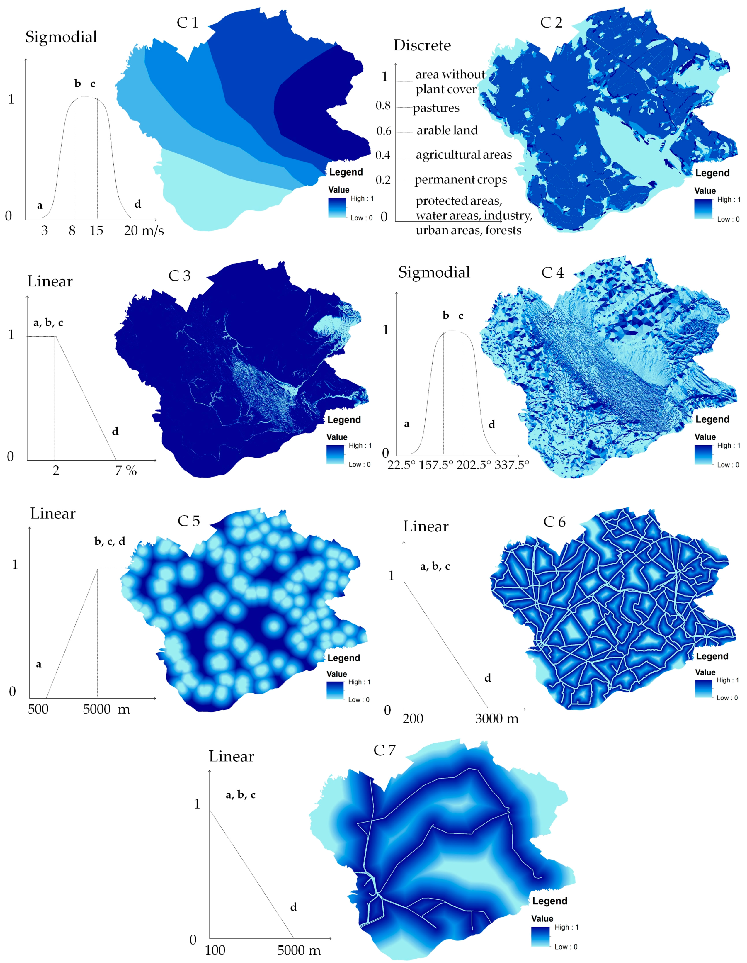
Given that the data on the criteria were collected in different ways and have different formats, it is necessary that data sets are standardized and converted into units that can be compared with each other. There are a number of approaches that can be used for attribute layers criteria to be comparable. In this case, with the criteria set whose elements are categorical values (Land use), the discrete classification is used, in which experts gave out value of the elements of fuzzy sets directly. In all other categories, which are the values of the gradual change from one location to another, elements of the set are standardized using fuzzy concept based on linear or sigmoidal membership function. For fuzzification scale ranges from 0 to 1 byte was used, where closer to 0 is the least, and closer to 1 the most appropriate value set in relation to the suitability of the location of the wind farm. Values with 0 are excluded from the analysis. Standardized criteria for evaluating the fuzzy membership functions and forms are shown in Table 3 and Figure 3.
It should be noted that the adopted criteria are not final and can be extended to a larger number of objective circumstances, taking into account application areas.
In this case study, when determining the weights of criteria, ten experts were involved with rich experience in the design of renewable energy sources and capital projects. Experts who have an experience of minimum five years in providing consulting services in the design of renewable energy sources were identified. After interviewing experts, the collected data are processed and aggregation of their opinions was executed.
In the first step of applying BWM experts used the following scale for the evaluation criteria: 1—No impact; 2—Very little impact; ...; 9—Very large impact. Seven experts took part in the research. The R-BWM was used to determine the weight coefficients of the criteria. After defining the criteria for evaluation, the experts also determined the best (B) and worst (W) criterion. On this basis, the experts determined the BO and OW matrices in which the preferences of the B and W over the criteria were considered for the remaining criteria from the defined set. Evaluation of the criteria was carried out using a scale [44]. The BO and OW matrices are presented in Table 4.
Using Equations (1)–(7) the evaluations in the BO and OW matrices were transformed into rough numbers, Table 5 and Table 6.
After transforming crisp numbers into rough numbers (Table 5 and Table 6), Equations (16) and (19) were used to transform the rough BO and OW matrices into aggregated rough BO and rough OW matrices, Table 7.
On the basis of the rough BO and OW matrices for criteria, the optimal values of the rough weight coefficients of the criteria were calculated. Based on model (18) the optimal values of the weight coefficients of the criteria were calculated, Table 8.
By solving the model (23) the value of is obtained, . The value of is used to determine the consistency ratio, Equation (28). Since we obtain the value of i.e., on the basis of the aggregated decisions of the experts, and they affect the interval of the RN, it is not possible to predefine the values of the consistency index . Using Equation (27), the values of the consistency index () is defined (CI = 0.0997).
3.4. The Summing of Pondered Maps into Suitability Map
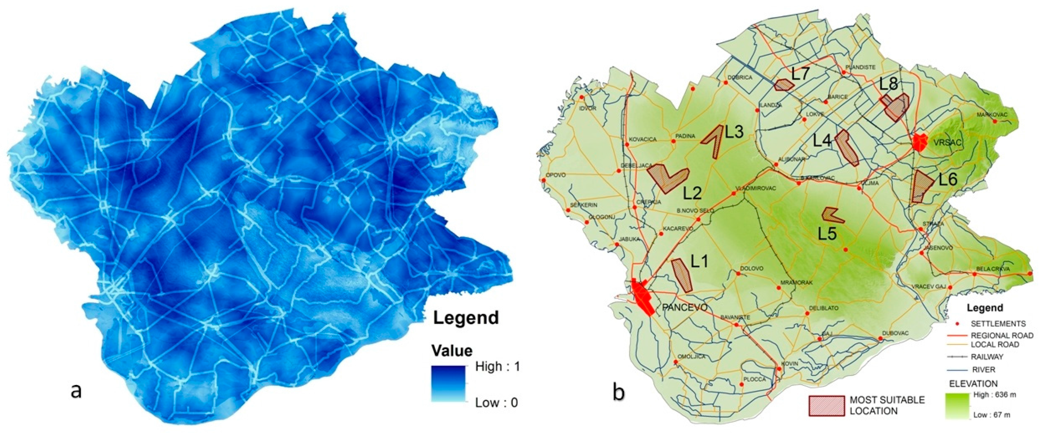
WLC method integrated into ArcGIS Advanced 10.2 software and ArcGIS Spatial Analyst extension were used in this step to sum normalized weighted criteria values. WLC aggregation of map criteria into the final suitability map of suitable location for wind farms is presented in the same value range from 0 to 1 was completed on the basis of the adopted criteria and particular weights determined by experts (Figure 4a). The greater cell values represent the area more suitable for the wind farm location.
The final step is to extract the cells with the highest values in the final suitability map. These are the areas which pixels have a value of 0.750 to 1 representing the most favorable locations for wind farms. There is 89.7 km2 of very suitable area for the construction of wind farms, obtained from the analysis in the Southern Banat, differentiated in eight locations (Figure 4b). These sites can be used as the main locations for the construction of wind farms in the Southern Banat.
3.5. The Location Ranking
Taking into account that the main purpose of this analysis is identification of the most suitable wind farm locations, this step involves ranking of the locations based on criteria parameters calculated using Zonal statistical algorithm ArcGis 10.2 software for each location (Table 9).
After identification of suitable locations, their ranking and selection of the best location using MAIRCA method is conducted. Locations evaluation and ranking were obtained using Expressions (29)–(43), Table 10.
Ranking of alternatives using MAIRCA method was carried out on the basis of the total value of the gap, whereby as the best alternative is taken one that has the lowest value of the gap, or the one that is closest to the ideal alternative. An alternative that is the worst is the one that has the highest value of the gap, or the one that is farthest from the ideal alternative. It is desirable that alternative has the lowest value of the total gap. Based on the conditions for ranking locations by using MAIRCA method it can be concluded that the best ranked alternative is L3.
4. Conclusions
This paper proposed the combination of rough sets in combination with multi-criteria methods within GIS software environment for the determination of suitable locations for the construction of wind farms. Developed rough BWM model that was used in this study is used to determine the weight or importance of each criterion. The WLC is used to sum up the weights and to identify the final suitable locations for wind farms. Application of GIS multi-criteria model in choosing locations for wind farms is carried out on a real case of micro region of the Southern Banat, Vojvodina, Serbia. The final suitability map is obtained defining eight locations that are most suitable for the construction of wind farms. In the following procedure, using rough MAIRCA model, the locations were ranked and the best one is proved to be location L3.
It should be pointed out that this procedure allows the inclusion of other criteria that were not included in this study. This model extends the theoretical framework of knowledge in location selection. The current problem is discussed using the new methodology, which creates the basis for further theoretical and practical upgrade.
Acknowledgments
The work reported in this paper is a part of the investigation within the research projects VA-TT/4/17-19 and VA/TT/3/17-19supported by the Ministry of Defence (Republic of Serbia) and the University of defence in Belgrade. This support is gratefully acknowledged.
Author Contributions
This research was carried out in collaboration between all authors. Ljubomir Gigović designed this research and collected data. Dragan Pamučar Zoran Bajić and Miljojko Janošević performed the simulation of the multi-criteria and the methodology. The discussions and analysis were carried out by all authors. All authors have read and approved the final manuscript.
Conflicts of Interest
The authors declare no conflict of interest.
References
- Aydin, N.Y.; Kentel, E.; Duzgun, S. GIS-based environmental assessment of wind energy systems for spatial planning: A case study from Western Turkey. Renew. Sustain. Energy. Rev. 2010, 14, 64–73. [Google Scholar] [CrossRef]
- Nadai, A. Planning ‘Siting’ and the local acceptance of wind power: Some lessons from the French case. Energy Policy 2007, 35, 15–26. [Google Scholar] [CrossRef]
- Wolsink, M. Near-shore wind power-Protected seascapes, environmentalists’ attitudes, and the technocratic planning perspective. Land Use Policy 2010, 27, 195–203. [Google Scholar] [CrossRef]
- Miller, A.; Ruopu, L. A Geospatial Approach for Prioritizing Wind Farm Development in Northeast Nebraska, USA. Int. J. Geo-Inf. 2014, 3, 68–79. [Google Scholar] [CrossRef]
- Global Wind Energy Council (GWEC). Wind Force 12, A Blueprint to Achieve 12% of the World’s Electricity from Wind Power by 2020; Greenpeace: Brussels, Belgium, 2005. [Google Scholar]
- Tegou, L.I.; Polatidis, H.; Haralambopoulos, D.A. Environmental management framework for wind farm siting: Methodology and case study. J. Environ. Manag. 2010, 91, 2134–2147. [Google Scholar] [CrossRef] [PubMed]
- Kang, R.; Zhang, T.; Tang, H.; Zhao, W. Adaptive Region Boosting method with biased entropy for path planning in changing environment. CAAI Trans. Intell. Technol. 2016, 1, 179–188. [Google Scholar] [CrossRef]
- Yeh, T.M.; Huang, Y.L. Factors in determining wind farm location: Integrating GQM, fuzzy DEMATEL and ANP. Renew. Energy 2014, 66, 159–169. [Google Scholar] [CrossRef]
- Douglas, N.G.; Saluja, G.S. Wind energy development under the UK non-fossil fuel and renewables obligations. Renew. Energy 1995, 6, 701–711. [Google Scholar] [CrossRef]
- Hansen, H. GIS-based multi-criteria analysis of wind farm development. In Proceedings of the 10th Scandinavian Research Conference on Geographical Information Science (ScanGIS), Stocholm, Sweden, 13–15 June 2005; pp. 75–85. [Google Scholar]
- Gourgiotis, A.; Kyriazopoulos, E. Electrical energy production from wind turbine Parks: The Finistere wind turbine Chart (France) and the Greek spatial planning experience (in Greek). In Proceedings of the INTERDISCIPLINARY Congress on “Education, Research, Technology. From Yesterday Till Tomorrow”, Athin, Greek, 21–25 July 2007; pp. 27–30. [Google Scholar]
- Pamučar, D.; Mihajlović, M.; Obradović, R.; Atanasković, P. Novel approach to group multi-criteria decision making based on interval rough numbers: Hybrid DEMATEL-ANP-MAIRCA model. Expert Syst. Appl. 2017, 88, 58–80. [Google Scholar] [CrossRef]
- Stevanovic, D.; Petkovic, P. Utility needs smarter Power Meters in Order to reduce economic Losses. Facta Univ. Ser. Electron. Energetics 2015, 28, 407–421. [Google Scholar] [CrossRef]
- Liu, H.; Wang, C.; Gao, Y. Scene-adaptive hierarchical data association and depth-invariant part-based appearance model for indoor multiple objects tracking. CAAI Trans. Intell. Technol. 2016, 1, 210–224. [Google Scholar] [CrossRef]
- Chang, N.B.; Parvathinathan, G.; Breeden, J.B. Combining GIS with fuzzy multicriteria decision-making for landfill siting in a fast-growing urban region. J. Environ. Manag. 2008, 87, 139–153. [Google Scholar] [CrossRef] [PubMed]
- Latinopoulos, D.; Kechagia, K. A GIS-based multi-criteria evaluation for wind farm site selection. A regional scale application in Greece. Renew. Energy 2015, 78, 550–560. [Google Scholar] [CrossRef]
- Ji, W.; Tang, L.; Li, D.; Yang, W.; Liao, Q. Video-based construction vehicles detection and its application in intelligent monitoring system. CAAI Trans. Intell. Technol. 2016, 1, 162–172. [Google Scholar] [CrossRef]
- Gigović, L.J.; Pamučar, D.; Božanić, D.; Ljubojević, S. Application of the GIS-DANP-MABAC multi-criteria model for selecting the location of wind farms: A case study of Vojvodina, Serbia. Renew. Energy 2017, 103, 501–521. [Google Scholar] [CrossRef]
- Gorsevski, P.V.; Cathcart, S.C.; Mirzaei, G.; Jamali, M.M.; Ye, X.; Gomezdelcampo, E. A group-based spatial decision support system for wind farm site selection in northwest Ohio. Energy Policy 2013, 55, 374–385. [Google Scholar] [CrossRef]
- Van Haaren, R.; Fthenakis, V. GIS-based wind farm site selection using spatial multicriteria analysis (SMCA): Evaluating the case for New York State. Renew. Sustain. Energy Rev. 2011, 15, 3332–3340. [Google Scholar] [CrossRef]
- Kim, J.Y.; Oh, K.Y.; Kang, K.S.; Lee, J.S. Site selection of offshore wind farms around the Korean Peninsula through economic evaluation. Renew. Energy 2013, 54, 189–195. [Google Scholar] [CrossRef]
- Gong, M.; Wang, S.; Liu, W.; Yan, J.; Jiao, L. Evolutionary computation in China: A literature survey. CAAI Trans. Intell. Technol. 2016, 1, 334–354. [Google Scholar] [CrossRef]
- Szurek, M.; Blachowski, J. A Gis-based method for wind farm location multi-criteria analysis. Min. Sci. 2014, 21, 65–81. [Google Scholar]
- Mekonnen, A.D.; Gorsevski, P.V. A web-based participatory GIS (PGIS) for offshore wind farm suitability within Lake Erie, Ohio. Renew. Sustain. Energy Rev. 2015, 41, 162–177. [Google Scholar] [CrossRef]
- Al-Yahyai, S.; Charabi, Y.; Gastli, A.; Al-Badi, A. Wind farm land suitability indexing using multi-criteria analysis. Renew. Energy 2012, 44, 80–87. [Google Scholar] [CrossRef]
- Watson, J.J.W.; Hudson, M.D. Regional Scale wind farm and solar farm suitability assessment using GIS-assisted multi-criteria evaluation. Landsc. Urban Plan. 2015, 138, 20–31. [Google Scholar] [CrossRef]
- Tsoutsos, T.; Tsitoura, I.; Kokologos, D.; Kalaitzakis, K. Sustainable siting process in large wind farms case study in Crete. Renew. Energy 2015, 75, 474–480. [Google Scholar] [CrossRef]
- Bagocius, V.; Zavadskas, E.K.; Turskis, Z. Multi-person selection of the best wind turbine based on the multi-criteria integrated additive-multiplicative utility function. J. Civ. Eng.Manag. 2014, 20, 590–599. [Google Scholar] [CrossRef]
- Jin, H.; Chen, Q.; Chen, Z.; Hu, Y.; Zhang, J. Multi-Leap Motion sensor based demonstration for robotic refine tabletop object manipulation task. CAAI Trans. Intell. Technol. 2016, 1, 104–113. [Google Scholar] [CrossRef]
- Azizi, A.; Malekmohammadi, B.; Jafari, H.R.; Nasiri, H.; Parsa, V.A. Land suitability assessment for wind power plant site selection using ANP-DEMATEL in a GIS environment: Case study of Ardabil province, Iran. Environ. Monit. Assess. 2014, 186, 6695–6709. [Google Scholar] [CrossRef] [PubMed]
- Janke, J.R. Multicriteria GIS modeling of wind and solar farms in Colorado. Renew. Energy 2010, 35, 2228–2234. [Google Scholar] [CrossRef]
- Dagdougui, H.; Ouammi, A.; Sacile, R. A regional decision support system for onsite renewable hydrogen production from solar and wind energy sources. Int. J. Hydrogen Energy 2011, 36, 14324–14334. [Google Scholar] [CrossRef]
- Gamboa, G.; Munda, G. The problem of wind farm location: A social multicriteria evaluation framework. Energy Policy 2007, 35, 1564–1583. [Google Scholar] [CrossRef]
- Baban, S.; Parry, T. Developing and applying a GIS-based approach to locating wind farms in the UK. Renew. Energy 2001, 24, 59–71. [Google Scholar] [CrossRef]
- Rodman, L.C.; Meentemeyer, R.K. A geographic analysis of wind turbine placement in Northern California. Energy Policy 2006, 34, 2137–2149. [Google Scholar] [CrossRef]
- Taghilo, A. Calculation of Wind Potential for Wind Power Construction Plant (Case Study in Zanjan Province); Tarbiat Modarres University: Tehran, Iran, 2011. [Google Scholar]
- Lee, K.H.; Jun, S.O.; Pak, K.H.; Lee, D.H.; Lee, K.W.; Park, J.P. Numerical optimization of site selection for offshore wind turbine installation using genetic algorithm. Curr. Appl. Phys. 2010, 10, S302–S306. [Google Scholar] [CrossRef]
- Xu, Y.; Dong, J.; Zhang, B.; Xu, D. Background modeling methods in video analysis: A review and comparative evaluation. CAAI Trans. Intell. Technol. 2016, 1, 43–60. [Google Scholar] [CrossRef]
- Denholm, P.; Hand, M.; Jackson, M.; Ong, S. Land-Use Requirements of Modern Wind Power Plants in the United States; National Renewable Energy Laboratory: Golden, CO, USA, 2009.
- Yang, Y.P.O.; Shieh, H.M.; Leu, J.D. A novel hybrid MCDM model combined with DEMATEL and ANP with applications. Int. J. Oper. Res. 2008, 5, 160–168. [Google Scholar]
- Rezaei, J. Best-worst multi-criteria decision-making method. Omega 2015, 53, 49–57. [Google Scholar] [CrossRef]
- Zhao, P.; Wang, J.; Xia, J.; Dai, Y.; Sheng, Y.; Yue, J. Performance evaluation and accuracy enhancement of a day-ahead wind power forecasting system in China. Renew. Energy 2012, 43, 234–241. [Google Scholar] [CrossRef]
- Xu, X.; Law, R.; Chen, W.; Tang, L. Forecasting tourism demand by extracting fuzzy Takagi-Sugeno rules from trained SVMs. CAAI Trans. Intell. Technol. 2016, 1, 30–42. [Google Scholar] [CrossRef]
- Rezaei, J.; Wang, J.; Tavasszy, L. Linking supplier development to supplier segmentation using Best Worst Method. Expert Syst. Appl. 2015, 42, 9152–9164. [Google Scholar] [CrossRef]
- Rezaei, J. Best-worst multi-criteria decision-making method: Some properties and a linear model. Omega 2016, 64, 126–130. [Google Scholar] [CrossRef]
- Zhu, G.N.; Hu, J.; Qi, J.; Gu, C.C.; Peng, J.H. An integrated AHP and VIKOR for design concept evaluation based on rough number. Adv. Eng. Inform. 2015, 29, 408–418. [Google Scholar] [CrossRef]
- Qazi, K.; Lam, H.K.; Xiao, B.; Ouyang, G.; Yin, X. Classification of epilepsy using computational intelligence techniques. CAAI Trans. Intell. Technol. 2016, 1, 137–149. [Google Scholar] [CrossRef]
- Pamučar, D.; Vasin, L.; Lukovac, L. Selection of railway level crossings for investing in security equipment using hybrid DEMATEL-MARICA Model. In Proceedings of the XVI International Scientific-Expert Conference on Railway, Railcon, Niš, Serbia, 9–10 October 2014; pp. 89–92. [Google Scholar]
- Gigović, L.J.; Pamučar, D.; Bajić, Z.; Milićević, M. The combination of expert judgment and GIS-MAIRCA analysis for the selection of sites for ammunition depot. Sustainability 2016, 8, 372. [Google Scholar] [CrossRef]
- Liu, H.; Tang, H.; Xiao, W.; Guo, Z.Y.; Tian, L.; Gao, Y. Sequential Bag-of-Words model for human action classification. CAAI Trans. Intell. Technol. 2016, 1, 125–136. [Google Scholar] [CrossRef]
- Malczewski, J. GIS and Multicriteria Decision Analysis; John Wiley and Sons: New York, NY, USA, 1999; p. 392. [Google Scholar]
- Zhai, L.Y.; Khoo, L.P.; Zhong, Z.W. A rough set enhanced fuzzy approach to quality function deployment. Int. J. Adv. Manuf. Technol. 2008, 37, 613–624. [Google Scholar] [CrossRef]
- Zhai, L.Y.; Khoo, L.P.; Zhong, Z.W. Towards a QFD-based expert system: A novel extension to fuzzy QFD methodology using rough set theory. Expert Syst. Appl. 2010, 37, 8888–8896. [Google Scholar] [CrossRef]
- Zhang, Q.; Xie, Q.; Wang, G. A survey on rough set theory and its applications. CAAI Trans. Intell. Technol. 2016, 1, 323–333. [Google Scholar] [CrossRef]
- Gigović, L.; Pamučar, D.; Bajić, Z.; Drobnjak, S. Application of GIS-Interval Rough AHP Methodology for Flood Hazard Mapping in Urban Areas. Water 2017, 9, 360. [Google Scholar] [CrossRef]
- Ren, J.; Liang, H.; Chan, F.T.S. Urban sewage sludge, sustainability, and transition for Eco-City: Multi-criteria sustainability assessment of technologies based on best-worst method. Technol. Forecast. Soc. Chang. 2017, 116, 29–39. [Google Scholar] [CrossRef]
- Zhong, Q.B.; Chen, F. Trajectory planning for biped robot walking on uneven terrain—Taking stepping as an example. CAAI Trans. Intell. Technol. 2016, 1, 197–209. [Google Scholar] [CrossRef]
- Guo, S.; Zhao, H. Fuzzy best-worst multi-criteria decision-making method and its applications. Knowl. Based Syst. 2017, 121, 23–31. [Google Scholar] [CrossRef]
- Institute of Multidisciplinary Research. 2017. Available online: http://www.imsi.bg.ac.rs/publications/?pub=2 (accessed on 16 March 2017).
- Provincial Secretariat for Energy and Mineral Resources. Wind Atlas in AP Vojvodina. Part of the Project: Wind Atlas on the Territory of AP Vojvodina, Novi Sad. 2008. Available online: http://www.psemr.vojvodina.gov.rs/index.php/studije/item/5-studije-potencijala-i-mogucnosti-koriscenja-energije-vetra-u-apv (accessed on 16 March 2017).
- Yang, W.; Sun, X.; Deng, W.; Zhang, C.; Liao, Q. Fourier Locally Linear Soft Constrained MACE for facial landmark localization. CAAI Trans. Intell. Technol. 2016, 1, 241–248. [Google Scholar] [CrossRef]
Figure 1.
Model for wind farm location selection.
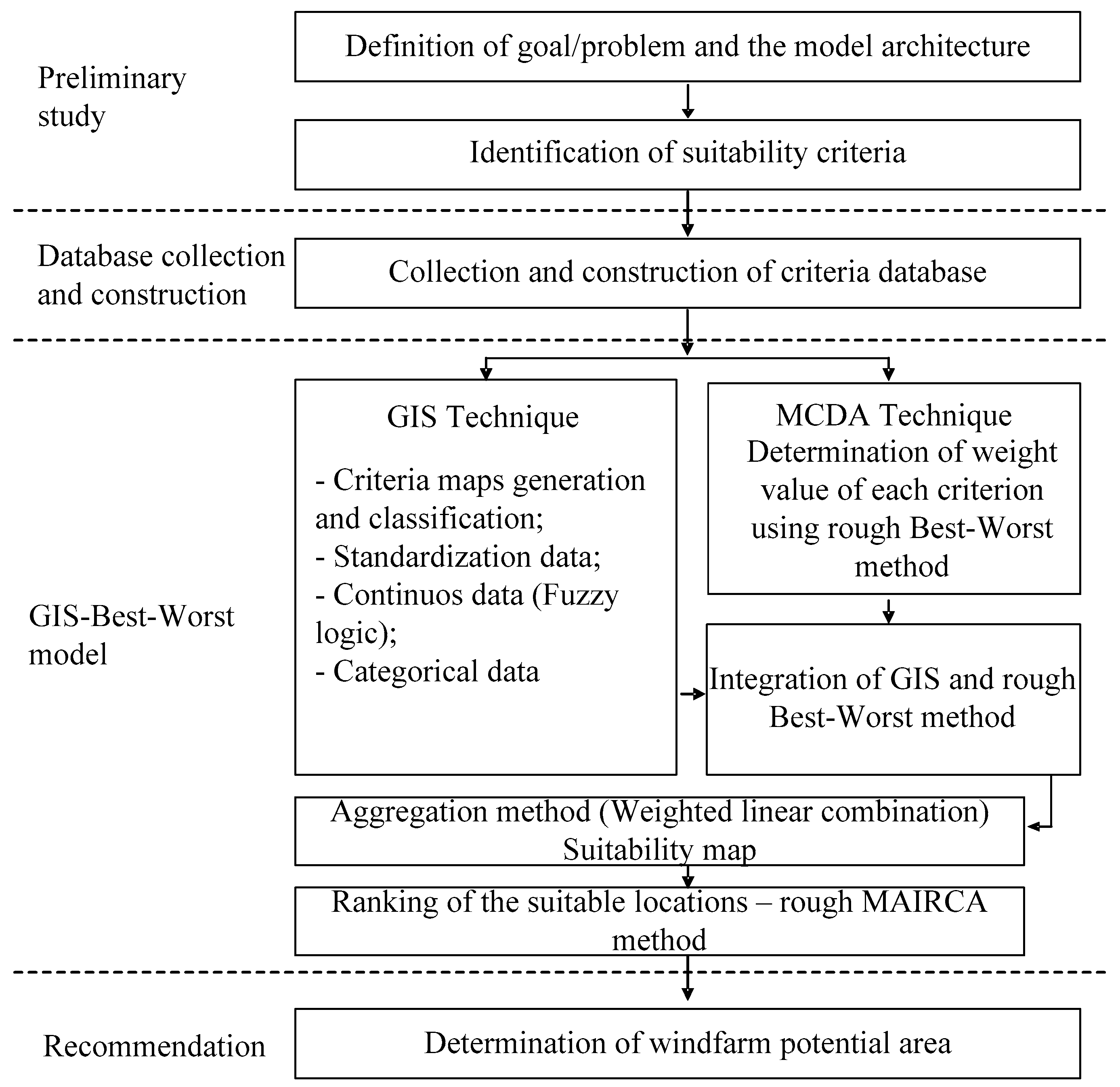
Figure 2.
The geographical position of study area.
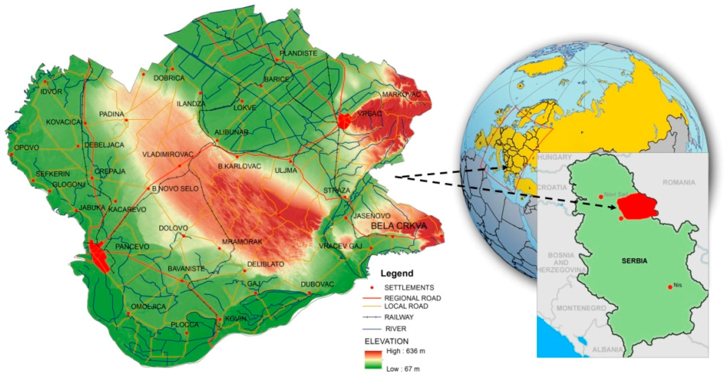
Figure 3.
Standardized criteria maps with fuzzy membership sets.

Figure 4.
Final suitability map (a) and most suitable locations (b) for the wind farm in the Southern Banat, Vojvodina, Serbia.
Figure 4.
Final suitability map (a) and most suitable locations (b) for the wind farm in the Southern Banat, Vojvodina, Serbia.

Table 1.
Values of the consistency index (CI).
| 1 | 2 | 3 | 4 | 5 | 6 | 7 | 8 | 9 | |
|---|---|---|---|---|---|---|---|---|---|
| CI () | 0.00 | 0.44 | 1.00 | 1.63 | 2.30 | 3.00 | 3.73 | 4.47 | 5.23 |
Table 2.
Criteria description.
| Crit. | Description |
|---|---|
| C1 | Wind speed average. The most important economic factor to consider when building a wind power plant on the wind speed at the monitored site. Locations with an average wind speed of more than 3 m/s are evaluated continuously, with the recommendation of the selection of sites to the average wind speed of 20 m/s. At speeds over 20 m/s it is possible that wind will damage the equipment. |
| C2 | Land cover/use. Land is one of the most important factors for energy investments. Wind farms should be installed in the area in which they negligibly interfere with existing land use outside protected areas, artificial surfaces, wetlands, aquatic and forest areas. The provided information on the land use is completed using CORINE project that provides sufficient comprehensiveness and consistency in European states. |
| C3 | Distance from main communication. The specificity of the installation equipment transport and subsequent maintenance of the wind farm is reflected in the need for secure road network to the location of wind turbines, with maximum use of the existing road network. In order to reduce the cost of transport is desirable that the distance from the roads outside the safety zone of 200 m, is as small as possible. |
| C4 | Slope. In a physical sense the wind farm should be located at suitable locations. Areas with steep slopes are generally considered less suitable, because of the extra costs of construction and maintenance. |
| C5 | Orientation Aspect. Orientation of slopes relative to the direction of the wind is an important criterion from the point of full utilization of the wind potential. It is desirable that the orientation of the slope on the location of the wind farm is toward the dominant wind blow. |
| C6 | Distance from urban places. Wind farms near urban areas can cause negative impacts on the local population. In order to minimize negative impacts on the environment it is recommended that wind farms are at the greatest possible distance from urban areas, at least 500 m. |
| C7 | Distance from power lines. One of the most important issues when it comes to reducing the cost of building wind farms is reducing costs for the construction of energy transmission infrastructure. When choosing a location, it is necessary to consider the availability of and access to existing electrical power lines. Due to the risk of potential accidents on power lines, the minimum distance of 100 m should be provided with adequate space between the columns and cable of power lines. |
Table 3.
Fuzzy standardization of criteria.
| Criteria | Fuzzy and Shape Membership Function | Control Points/Value Points | Final Utility |
|---|---|---|---|
| Wind speed (C1) | Sigmoidal Symmetric | A = 3 m/s c = 8 m/s | 0–3 m/s equal 0, 3–8 m/s between 0–1, 8–15 m/s equal l, 15–20 m/s between 1–0, more than 20 m/s equal to 1 |
| b = 15 m/s d = 20 m/s | |||
| Land use (C2) | Discrete categorical data | protected areas, water areas, industry, urban areas, forests equal 0, permanent agricultural areas equal 0.2, diverse agricultural areas equal 0.4, arable land equals 0.6, pastures equal 0.8, the area with minor and without plant cover equals 1 | |
| Distance from communications (C3) | Linear | c = 200 m | 0–200 m equal 0, 100–3000 m between 1–0, more than 3000 m equal to 0 |
| Monotonically decreasing | d = 3000 m | ||
| Slope (C4) | Linear | c = 2% | 0–2% equal 1, 2–7% between 1–0, more than 7% equal to 0 |
| Monotonically decreasing | d = 7% | ||
| Orientation aspect (C5) | Sigmoidal | a = 22.5° c = 202.5° | 337,5–22,5° equal 0, 22.5–157.5° between 0–1, 157.5–202.5° equal 1, 202.5–337.5° between 1–0 |
| Symmetric | b = 157.5° d = 337.5° | ||
| Distance from urban areas (C6) | Linear | a = 500 m | 0–500 m equal 0, 500–5000 m between 0–1, more than 5000 m equal to 1 |
| Monotonically increasing | b = 5000 m | ||
| Distance from power lines (C7) | Linear | c = 100 m | 0–100 m equal 0, 100–5000 m between 1–0, more than 5000 m equal to 0 |
| Monotonically decreasing | d = 5000 m | ||
Table 4.
The BO and OW expert evaluation matrices.
| Best: C1 | Expert Evaluation (E1, E2, ..., E7) | Worst: C3 | Expert Evaluation (E1, E2, ..., E7) |
|---|---|---|---|
| C1 | 1; 1; 1; 1; 1; 1; 1; 1; 1 | C1 | 9; 8; 9; 9; 9; 8; 8; 8; 9 |
| C2 | 5; 5; 4; 5; 4; 4; 4; 4; 5 | C2 | 3; 4; 3; 3; 3; 4; 3; 3; 3 |
| C3 | 9; 8; 8; 9; 8; 9; 9; 9; 9 | C3 | 1; 1; 1; 1; 1; 1; 1; 1; 1 |
| C4 | 2; 3; 2; 2; 2; 2; 2; 2; 2 | C4 | 8; 7; 8; 8; 8; 8; 8; 8; 8 |
| C5 | 4; 2; 4; 4; 4; 4; 2; 2; 4 | C5 | 6; 5; 6; 6; 6; 6; 5; 5; 6 |
| C6 | 8; 7; 7; 7; 7; 7; 8; 8; 8 | C6 | 2; 2; 2; 3; 2; 2; 2; 2; 2 |
| C7 | 6; 7; 6; 6; 6; 7; 6; 6; 6 | C7 | 2; 3; 2; 2; 2; 3; 3; 3; 2 |
Table 5.
Rough BO matrices.
| Best: C1 | Expert Evaluation (E1, E2, ..., E7) |
|---|---|
| C1 | [1, 1]; [1, 1]; [1, 1]; [1, 1]; [1, 1]; [1, 1]; [1, 1] |
| C2 | [4.57, 5]; [4.57, 5]; [4, 4.57]; [4.57, 5]; [4, 4.57]; [4, 4.57]; [4, 4.57] |
| C3 | [8.71, 9]; [8, 8.71]; [8, 8.71]; [8.71, 9]; [8.71, 9]; [8.71, 9]; [8.71, 9] |
| C4 | [2, 2.14]; [2.14, 3]; [2, 2.14]; [2, 2.14]; [2, 2.14]; [2, 2.14]; [2, 2.14] |
| C5 | [3.43, 4]; [2, 3.43]; [3.43, 4]; [3.43, 4]; [3.43, 4]; [2, 3.43]; [3.43, 4] |
| C6 | [7.43, 8]; [7, 7.43]; [7, 7.43]; [7, 7.43]; [7, 7.43]; [7, 7.43]; [7, 7.43] |
| C7 | [6, 6.29]; [6.29, 7]; [6, 6.29]; [6, 6.29]; [6.29, 7]; [6, 6.29]; [6, 6.29] |
Table 6.
Rough OW matrices.
| Worst: C3 | Expert Evaluation (E1, E2, ..., E7) |
|---|---|
| C1 | [8.57, 9]; [8, 8.57]; [8.57, 9]; [8.57, 9]; [8, 8.57]; [8.57, 9]; [8.57, 9] |
| C2 | [3, 3.29]; [3.29, 4]; [3, 3.29]; [3, 3.29]; [3.29, 4]; [3, 3.29]; [3, 3.29] |
| C3 | [1, 1]; [1, 1]; [1, 1]; [1, 1]; [1, 1]; [1, 1]; [1, 1] |
| C4 | [7.86, 8]; [7, 7.86]; [7.86, 8]; [7.86, 8]; [7.86, 8]; [7.86, 8]; [7.86, 8] |
| C5 | [5.71, 6]; [5, 5.71]; [5.71, 6]; [5.71, 6]; [5.71, 6]; [5, 5.71]; [5.71, 6] |
| C6 | [2, 2.14]; [2, 2.14]; [2, 2.14]; [2.14, 3]; [2, 2.14]; [2, 2.14]; [2, 2.14] |
| C7 | [2, 2.43]; [2.43, 3]; [2, 2.43]; [2, 2.43]; [2.43, 3]; [2.43, 3]; [2, 2.43] |
Table 7.
Aggregated rough BO and rough OW matrices.
| Best: C1 | RN | Worst: C3 | RN |
|---|---|---|---|
| C1 | [1.00, 1.00] | C1 | [8.41, 8.88] |
| C2 | [4.24, 4.76] | C2 | [3.08, 3.49] |
| C3 | [8.51, 8.92] | C3 | [1.00, 1.00] |
| C4 | [2.02, 2.27] | C4 | [7.73, 7.98] |
| C5 | [3.02, 3.84] | C5 | [5.51, 5.92] |
| C6 | [7.06, 7.51] | C6 | [2.02, 2.27] |
| C7 | [6.08, 6.49] | C7 | [2.18, 2.67] |
Table 8.
Optimal values of the criteria.
| Criterion | Weights | Rank |
|---|---|---|
| C1 | [0.364, 0.416] | 1 |
| C2 | [0.114, 0.127] | 4 |
| C3 | [0.037, 0.060] | 7 |
| C4 | [0.235, 0.339] | 2 |
| C5 | [0.159, 0.253] | 3 |
| C6 | [0.044, 0.058] | 6 |
| C7 | [0.048, 0.059] | 5 |
Table 9.
Initial matrix for location evaluation.
| Locations | Criteria | ||||||
|---|---|---|---|---|---|---|---|
| C1 | C2 | C3 | C4 | C5 | C6 | C7 | |
| L1 | [0.38, 0.42] | [0.74, 0.80] | [0.97, 1.00] | [0.48, 0.55] | [0.97, 1.02] | [0.62, 0.69] | [0.82, 0.86] |
| L2 | [0.47, 0.53] | [0.75, 0.81] | [0.96, 1.00] | [0.65, 0.69] | [0.94, 1.00] | [0.61, 0.68] | [0.73, 0.78] |
| L3 | [0.46, 0.54] | [0.75, 0.80] | [0.97, 1.00] | [0.42, 0.48] | [0.95, 1.00] | [0.80, 0.86] | [0.80, 0.85] |
| L4 | [0.59, 0.63] | [0.74, 0.80] | [0.97, 1.00] | [0.51, 0.58] | [0.91, 0.98] | [0.62, 0.66] | [0.48, 0.52] |
| L5 | [0.58, 0.62] | [0.74, 0.79] | [0.97, 1.00] | [0.30, 0.35] | [0.94, 1.01] | [0.55, 0.61] | [0.49, 0.55] |
| L6 | [0.75, 0.81] | [0.75, 0.81] | [0.96, 1.00] | [0.64, 0.69] | [0.76, 0.82] | [0.63, 0.71] | [0.80, 0.85] |
| L7 | [0.57, 0.63] | [0.70, 0.76] | [0.97, 1.00] | [0.71, 0.75] | [0.69, 0.75] | [0.62, 0.68] | [0.81, 0.86] |
| L8 | [0.56, 0.64] | [0.73, 0.80] | [0.96, 1.00] | [0.60, 0.65] | [0.88, 0.93] | [0.63, 0.69] | [0.71, 0.78] |
Table 10.
Location rankings using MAIRCA method.
| Location | Rough Value | Rank |
|---|---|---|
| L1 | [0.0233, 0.0666] | 3 |
| L2 | [0.0295, 0.0505] | 6 |
| L3 | [0.0135, 0.0658] | 1 |
| L4 | [0.0287, 0.0808] | 5 |
| L5 | [0.0437, 0.0609] | 7 |
| L6 | [0.0238, 0.0818] | 4 |
| L7 | [0.0447, 0.0588] | 8 |
| L8 | [0.0217, 0.0185] | 2 |
© 2017 by the authors. Licensee MDPI, Basel, Switzerland. This article is an open access article distributed under the terms and conditions of the Creative Commons Attribution (CC BY) license (http://creativecommons.org/licenses/by/4.0/).
Share and Cite
MDPI and ACS Style
Pamučar, D.; Gigović, L.; Bajić, Z.; Janošević, M. Location Selection for Wind Farms Using GIS Multi-Criteria Hybrid Model: An Approach Based on Fuzzy and Rough Numbers. Sustainability 2017, 9, 1315. https://doi.org/10.3390/su9081315
AMA Style
Pamučar D, Gigović L, Bajić Z, Janošević M. Location Selection for Wind Farms Using GIS Multi-Criteria Hybrid Model: An Approach Based on Fuzzy and Rough Numbers. Sustainability. 2017; 9(8):1315. https://doi.org/10.3390/su9081315
Chicago/Turabian StylePamučar, Dragan, Ljubomir Gigović, Zoran Bajić, and Miljojko Janošević. 2017. "Location Selection for Wind Farms Using GIS Multi-Criteria Hybrid Model: An Approach Based on Fuzzy and Rough Numbers" Sustainability 9, no. 8: 1315. https://doi.org/10.3390/su9081315
Note that from the first issue of 2016, this journal uses article numbers instead of page numbers. See further details here.