Article

Evaluating the Comprehensive Performance of Demand Response for Commercial Customers by Applying Combination Weighting Techniques and Fuzzy VIKOR Approach

School of Economics and Management, North China Electric Power University, Beijing 102206, China
*
Author to whom correspondence should be addressed.
Sustainability 2017, 9(8), 1332; https://doi.org/10.3390/su9081332
Submission received: 29 June 2017 / Accepted: 6 July 2017 / Published: 31 July 2017
(This article belongs to the Section Energy Sustainability)

Abstract

:
In order to guarantee the sustainability of power industries, demand response is widely developed in China with the improvement of power markets. Massive potential flexible resources in the commercial sector are valuable to carry out continuous demand response programs. This paper presented a hybrid framework to evaluate the performance of such programs. Considering that assessment processes involve multiple decisions for massive criteria under fuzzy conditions, we proposed a fuzzy multi-criteria decision making model to evaluate the performance of commercial demand response based on the concepts of a fuzzy Vlsekriterijumska Optimizacijia I Kompromisno Resenje method and a L2-metric distance. The weighting determination process in the model was modified by integrating subjective opinions and objective information according to a fuzzy Analytic Hierarchy Process and Criteria Importance Through Intercriteria Correlation methods. Then a comprehensive evaluation index system for demand response performance was established by using a fuzzy Delphi method based on experts’ opinions, including the five aspects of economy, society, technology, environment and management. Finally, the practicality of the proposed hybrid framework was verified through an empirical analysis of five such programs in Chinese commercial buildings. Their comprehensive performances were ranked effectively. Sub-criteria affiliated with society and environment should be more attention than the other evaluation criteria based on experts’ judgments and objective information. Moreover, a set of sensitivity analyses were performed to confirm the robustness and effectiveness of the proposed framework and the evaluation results. The study findings can offer references for the improvement of demand response and relevant policy formulation.

1. Introduction

Conventional power industries relying heavily on fossil fuels have caused increasing environmental ecological issues worldwide, such as pollutant emissions, greenhouse effect, water quality degradation and fog and haze weather [1]. With a growing consensus of sustainability development, renewable energy sources (RES) are introduced into power systems to replace depleted fossil fuels and realize energy transition, which are recognized as a global trend of power industries. China, for example, committed to increase a proportion of RES power generations to around 40% by 2020 [2]. However, a lot of uncertain RES power generations, especially wind and solar, may lead to potential imbalances between supply and demand on power systems [3,4]. In order to process the problem, flexibility at the demand side is recommended to introduce into the power grids as more as possible. Demand response (DR) can lead to variations in energy consumption habits of users in response to different electric prices over time or in the presence of economic incentives. It is increasingly regarded as an elegant solution to compensate these imbalances and improve energy efficiency [5,6]. Massive potential flexible resources can be aggregated to reduce peak loads and handle the variability of RES power generations [7]. Moreover, DR is an essential ingredient to decrease traditional power generations by adjustment of electricity demand and utilization of flexible resources [8,9].
DR programs have been researched and implemented widely in the industrial and commercial sectors worldwide [10]. For instance, many DR programs in the United States were provided by the New York Independent System Operator in which participants can change their loads based on price fluctuations or emergency signals [11]. In Europe, various DR programs were studied or put into practice [12,13], such as in the cases of Germany [14], Sweden [15], the United Kingdom [16] and Italy [17]. Torriti [13] summarized the researches on these programs in the above European countries, containing DR status quo, economic potential and policy levels. In China, the National Development and Reform Commission announced the “Electricity Demand-side Management Measures” in 2010, which aimed to promote the DR programs in the industrial sector [18]. Many regions were selected as pilots to conduct such programs with the support of special financial funds since 2012, including Suzhou, Beijing, Foshan, Tangshan and Shanghai cities [19]. Following the industrial structure adjustment, commercial customers have been strong electric consumers and can account for the major increment of Chinese final electricity consumption. A lot of commercial flexible resources in lighting, electronic equipment, heating-ventilation and air conditioning (HVAC) systems should play a significant role in maintaining electricity balances and offering a series of options for demand management [20]. Thus, many DR programs should be designed and performed for commercial users to control the flexibility through deploying smart meters widely, such as time-of-use tariff mechanisms, demand side bidding and interruptible load management [21].
It is noted that implementing DR programs needs not only deployment of required automated devices, but also a thorough evaluation of their performance. In order to support decisions, it is essential to provide insight into the performance of these programs. Some researchers have already analyzed these assessments on some countries and regions, such as Conchado [22] for Spain, FERC [23] for the USA, Klaassen [24] for Netherlands, Cepeda [25] for France. Pinson [7] offered an overview of the benefits and challenges for DR programs from the perspectives of operation, plans, economy, market regulations and business cases. Nolan [26] summarized the DR evaluation methodologies from the aspects of production cost simulation and capacity value assessment. Previous researchers paid much attention to the DR performance in energy system operation, economic feasibility and environment protection, including energy cost saving [22], flexible load aggregation [27], peak load reductions [28], the potential profits for project participants [29], RES penetration [30] and CO2 emissions [31]. Gils [32] assessed demand response potential of the 40 European countries in all consumer sectors, involving shiftable loads, temporal availability and geographic allocation for flexible loads. However, these relevant researches with a few criteria are still relatively insufficient to reflect DR performance completely. It is essential to establish an evaluation system to measure the comprehensive performance of DR programs reasonably.
For comprehensive evaluation, a sustainable perspective is introduced to develop the evaluation system of DR performance. Based on a traditional sustainability paradigm, it should contain three dimensions: economic, social and environmental [33]. Because the flexible resources of commercial customers are more dispersed than these of industrial users, massive elements on technology and management should be properly considered at the basis of relevant electric consumption processes. These elements may impact on customers’ response extremely, containing automated equipment construction and operation, technical standard implementation, a loss of productivity, prior experiences [
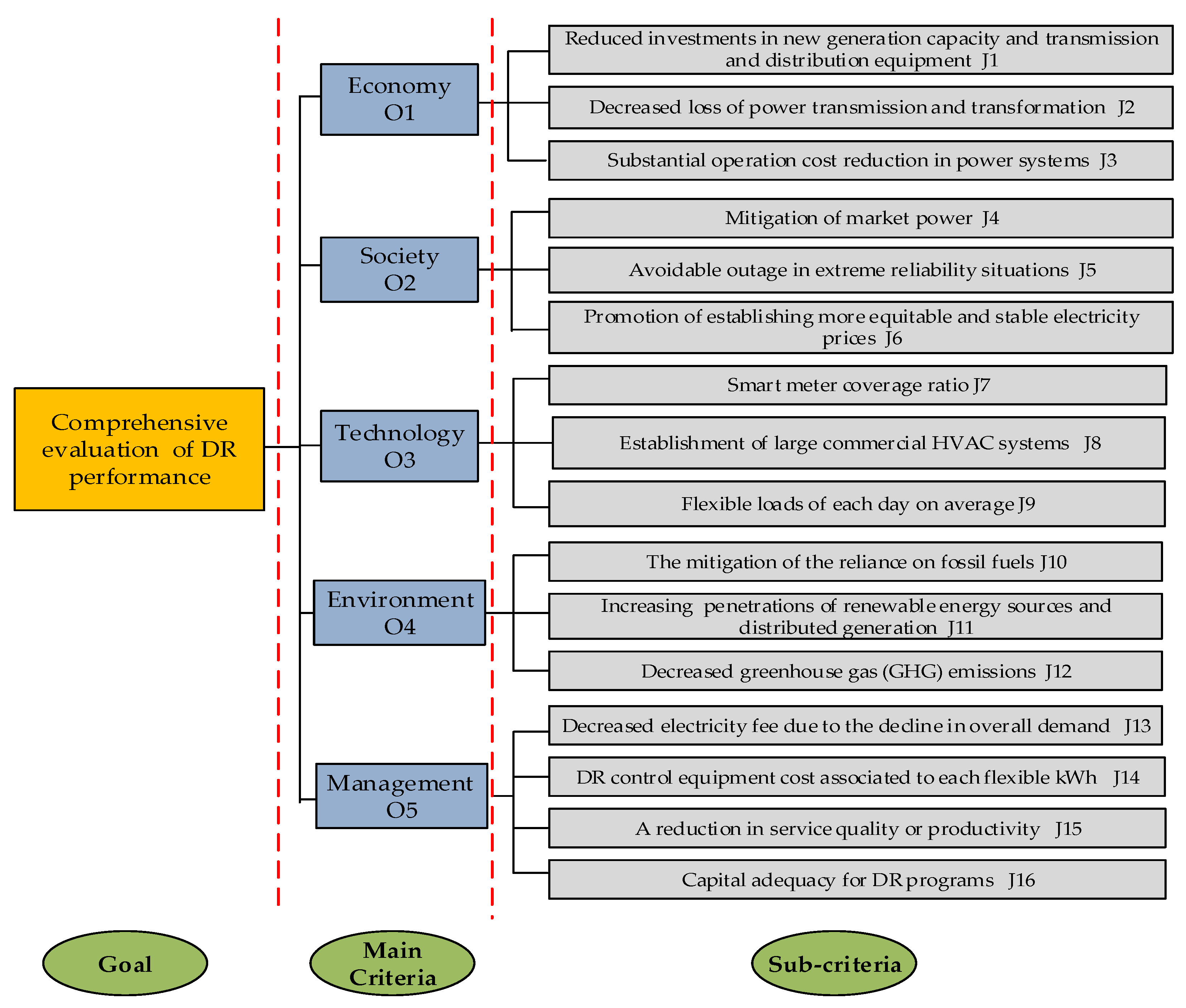
32,34]. Hence, a comprehensive evaluation index system can be formed to reveal the performance of commercial DR from five dimensions, namely economy, society, technology, environment and management. An initial index system can be built firstly according to existing literatures. In order to ensure the rationality of the evaluation index system, a fuzzy Delphi method can be applied to remove redundant criteria according to experts’ linguistic ratings.
In view of the fact that the performance evaluation of DR involves many dimensions, a multiple criteria decision making (MCDM) technique should be proposed to conduct the evaluation processes. A variety of MCDM methods have been applied to assess the performances of enterprises or projects, such as the entropy weight method [35], the analytic hierarchy process (AHP), the technique for order preference by similarity to an ideal solution (TOPSIS) [36] and the elimination et choice translating reality (ELECTRE) [37]. Based on previous research, we introduced a hybrid MCDM technique to the performance evaluation of commercial DR programs. Vlsekriterijumska Optimizacija I Kompromisno Resenje (VIKOR) method, put forward by Opricovic firstly [38], has been regarded as a compensatory aggregation approach to handle discrete MCDM issues with conflicting and noncommensurable criteria. This method focuses on proposing acceptable compromise solutions closed to the ideal state and sorting a set of evaluation alternatives, which has been widely applied to simply multi criteria of complex decision systems and handle the balance between the overall benefits and individual satisfaction in real MCDM issues [39,40,41]. However, experts often fail to provide precise decision makings for criteria performance due to lack of experience and accurate data. The decision making information, such as important, poor, good and so on, is almost impossible to describe through conventional quantitative expressions. To process vague decisions, a fuzzy VIKOR method was developed at the basis of a fuzzy logic theory [42,43,44]. Linguistic ratings given by decision makers were expressed as triangular fuzzy numbers (TFNs) to perform calculations. Then to better effectively calculate distances between TFNs as well as sort priorities of alternatives with precise numbers, a L2-metric distance approach was applied to modify the traditional aggregating function. Moreover, a combination weight technique based on fuzzy AHP and Criteria Importance Through Intercriteria Correlation (CRITIC) methods was developed to promote the weighting determination processes for the fuzzy VIKOR.
Primary contributions in this paper are:
  • A comprehensive index system for DR performance in the commercial sector was formed firstly, including the five perspectives of economy, society, technology, environment and management. The fuzzy Delphi method with easy implementation was applied to select rational evaluation criteria based on decision makers’ opinions.
  • A hybrid MCDM model were established firstly to assess the comprehensive performance of commercial DR. A modified fuzzy VIKOR method with L2-metric distances was firstly developed. The fuzzy AHP and CRITIC methods were combined to innovate the weighting determination. Due to the application of the fuzzy logic theory, this model may effectively capture fuzziness of human decisions. The modified fuzzy VIKOR with the characteristics of clear concepts can measure precise distances between TFNs to better process conflicting criteria in complex decision-making systems. The combination weight technique not only contains decision makers’ judgments, but also utilizes objective information for all alternatives. It can ensure the rationality and practicality of weighting determination.
  • Considering that decision makers with diverse professional backgrounds may give different judgments, we conducted a set of sensitivity analyses to verify the impacts of criteria weights and parameter fluctuations on performance evaluation results. The detailed discussions can illuminate the robustness of the proposed framework under various cases. This is the first study that analyzes the important of evaluation criteria for commercial DR performance by changing the weights. The analysis results can contribute to help experts’ decision makings on DR programs.
The remainder of this paper is organized as follows. Section 2 describes the basic methodology; the research framework is presented in detail in Section 3; Section 4 establishes a comprehensive evaluation index system for commercial DR performance. In Section 5, an empirical analysis is illustrated by carrying out the DR performance assessment of five commercial buildings in China. We perform sensitivity analyses and discuss the results in Section 6. Conclusions are drawn in the final section.

2. Methodology

We introduce relevant mathematics methods briefly, including the fuzzy logic theory, the fuzzy AHP, the CRITIC and the modified fuzzy VIKOR methods, which will be employed to propose a hybrid research framework.

2.1. Fuzzy Logic Theory

The fuzzy logic theory, introduced by Zadeh [45] in 1965, is used to cope with vague linguistic information from human decisions in a real world. Fuzzy sets are defined to map ambiguous linguistic ratings into precise numerical terms. A fuzzy set is featured by a membership function with continuous grades. Each criterion can obtain a membership value among [0,1] to express its degree belonging to the fuzzy set. If a membership value is one, the criterion belongs to the set absolutely. If a membership value is zero, the criterion doesn’t belong to the set. If a membership value is between zero and one, the criterion belongs to the set partially. Besides, some linguistic ratings such as “poor”, “fair” and “good” can be described as a series of numerical intervals.
A TFN, denoted by a triplet A ˜ = ( a L ,   a M ,   a R ) , is used widely in fuzzy applications. a L ,   a M and a R are the minimum value, the middle value and the maximum value, which are all crisp numbers and < a L a M a R < + . Let x be a vague variable, then its membership function μ A ˜ ( x ) can be expressed as:
μ A ˜ ( x ) = { x a L a M a L , a L x < a M a R x a R a M , a M x a R 0 o t h e r w i s e ,
Suppose A ˜ 1 = ( a 1 L ,   a 1 M ,   a 1 R ) and A ˜ 2 = ( a 2 L ,   a 2 M ,   a 2 R ) are TFNs, some basic operations are:
A ˜ 1 A ˜ 2 = ( a 1 L + a 2 L ,   a 1 M + a 2 M ,   a 1 R + a 2 R ) ,
A ˜ 1 A ˜ 2 = ( a 1 L a 2 L ,   a 1 M a 2 M ,   a 1 R a 2 R ) ,
A ˜ 1 A ˜ 2 = ( a 1 L × a 2 L ,   a 1 M × a 2 M ,   a 1 R × a 2 R ) ,
A ˜ 1 1 = ( 1 / a 1 R ,   1 / a 1 M ,   1 / a 1 L ) ,
The distance between A ˜ 1 = ( a 1 L ,   a 1 M ,   a 1 R ) and A ˜ 2 = ( a 2 L ,   a 2 M ,   a 2 R ) can be computed easily based on the L2-metric distance approach, which can better consider the different importance of the minimum value, the middle value and the maximum value of a TFN [46].
d ( A ˜ 1 , A ˜ 2 ) = { [ ( a 1 L a 2 L ) 2 + 4 × ( a 1 M a 2 M ) 2 + ( a 1 R a 2 R ) 2 ] / 6 } 1 / 2 ,
Human often make vague answers instead of accurate values in MCDM processes. Qualitative linguistic values and the fuzzy set theory are suitable to evaluate performances rather than traditional numerical methods under fuzzy circumstances. As we know, the fuzzy logic theory has been gathered into a lot of traditional MCDM methods, such as fuzzy AHP, fuzzy Delphi, fuzzy TOPSIS, and fuzzy VIKOR methods. At the aim of comparing alternatives and obtaining precise information, a center of area (COA) defuzzification method is introduced to compute a best non-fuzzy performance (BNP) number [47]. Let A ˜ = ( a L ,   a M ,   a R ) be a TFN, its BNP value B ( A ˜ ) is:
B ( A ˜ ) = ( a R a L ) + ( a M a L ) 3 + a L ,

2.2. Fuzzy Delphi Method

The Delphi method, put forward by Dalky and Helmer [48], is an important expert survey technique with the merits of anonymous responses, controlled and iterative feedback and statistical group responses. In order to make a consistent judgment, decision makers can get feedback information and revise previous opinions by several rounds of written communications. The traditional method has been widely used in economic forecasting, management strategy evaluation and public policy analysis etc. However, in terms of processing uncertain decision information, it has many shortcomings, such as long feedback time, high decision cost, low convergence rate, the possibility of distorting experts’ opinions. Thus, the fuzzy logic theory is introduced by Murry [49] to improve the traditional method. The fuzzy Delphi method allows experts to express their opinions thought linguistic variables and has the following benefits compared with the traditional method: (a) Subjective judgments are reserved entirely to prevent distortion of decision results. (b) Consistent comments may be received by one round of a questionnaire survey instead of multiple rounds of modifications, which is considered to improve decision efficiency. Thus, the fuzzy Delphi method is applicable to recognize vital evaluation criteria for commercial DR performance. Calculation procedures are shown as:
Step 1: Collect opinions on evaluation criteria importance. Decision makers should give judgments on the relative importance of the m criteria, which is represented by several numerical intervals ranging from 0 to 10. 0 and 10 mean “extremely unimportant” and “extremely important”, respectively. The maximum of the numerical interval denotes optimistic cognition, whereas the minimum one denotes pessimistic cognition.
Step 2: Assemble several optimistic TFNs and pessimistic TFNs to reveal overall decisions. The maximum and minimum values of the number interval for each criterion are sorted out respectively. Their corresponding geometric mean values are computed. Then an optimistic TFN O j = ( L j o , M j o , R j o ) and a conservative TFN P j = ( L j p , M j p , R j p ) for criterion j can be assembled. L j o and L j p are the minimum values of optimistic cognition and pessimistic cognition given by all decision makers respectively. R j o and R j p are the maximum values of optimistic cognition and pessimistic cognition. M i o and M i p respectively correspond to the geometric mean values of all decision makers’ optimistic cognition and pessimistic cognition.
Step 3: Check the consistency of all decision makers’ opinions. A consensus significance value G j is introduced to determine a consistent degree of each criterion j. The larger the G j value is, the more consistent the opinions are. It can be calculated by:
  • If L j o R j p , criterion j reaches a consensus, the G j value can be:
    G j = M j o + M j p 2 ,
  • If L j o < R j p , G j can be calculated according to the gray interval T j = R j p L j o .
    • If T j is smaller than the interval H j = R j o M j p , the opinions for criterion j are a consensus
      G j = M j o × R j p L j o × M j p ( R j p M j p ) + ( M j o L j o ) ,
    • If T j is greater than H j , the opinions for criterion j are not a consensus. Steps 1 to 3 need to be conducted repeatedly until all opinions reach a consensus.
Step 4: Choose vital criteria by setting a threshold θ . The θ value can be determined by the decision makers to reflect a minimum level of the acceptable consistency. If G j is lower than θ , the criterion j will be eliminated from an evaluation index system.

2.3. Fuzzy VIKOR Method

Conventional VIKOR method is usually employed for multi-criteria optimization of complex systems. Its obvious characteristics are that a multi-criteria ranking index is defined based on the special measurement of closeness to ideal points and the proposed compromise solutions offer the balance between maximization of whole utility and minimization of individual regret [50]. Its basic idea lies in building an aggregated function that can reveal distances from the positive and negative ideal points. In order to cope with subjectivity and uncertainty of decision makings, the fuzzy logic theory is posited into the conventional VIKOR. The fuzzy VIKOR is much more rational to rank various alternatives including conflicting criteria in a real decision environment. In this section, the L2-metric distance approach is introduced to modify the normal aggregated function.
Assume that there are m alternatives, n criteria and K decision makers in a MCDM issue. Each alternative is evaluated with relative to the n criteria. Considering imprecision and uncertainty of subjective opinions, decision makers assess criteria performance based on linguistic variables in Table 1. Let x ˜ i j k = ( x i j k L , x i j k M , x i j k R ) be the fuzzy performance of the alternative i with respect to criterion j given by decision maker k, i = 1 , 2 , , m , j = 1 , 2 , , n  and k = 1 , 2 , , K .
More procedures of the modified approach are shown as:
Step 1: Establish an initial fuzzy decision matrix.
These fuzzy ratings of alternatives should be aggregated as:
x ˜ i j = ( x i j L , x i j M , x i j R ) ,
where x i j L = 1 K k = 1 K x i j k L , x i j M = 1 K k = 1 K x i j k M and x i j R = 1 K k = 1 K x i j k R .
Then a MCDM issue can be presented concisely in a fuzzy matrix by assembling these aggregated fuzzy ratings, as is:
X = [ x ˜ 11 x ˜ 12 x ˜ 1 n x ˜ 21 x ˜ 22 x ˜ 2 n x ˜ m 1 x ˜ m 2 x ˜ m n ] ,
Step 2: Standardize the initial fuzzy decision matrix.
At the aim of avoiding criteria dimensional differences, it is vital to normalize the aggregated rating values. An evaluation index system usually contains benefit-type criteria with the higher the better and cost-type criteria with the lower the better. The linear scaling transformation method [52] is applicable to transform the aggregated ratings into comparable format. Let Y = [ y ˜ i j ] m × n denote a normalized fuzzy decision matrix. The normalization processes are as below.
For a benefit-type criterion
y ˜ i j = ( y i j L , y i j M , y i j R ) = ( x i j L u i + , x i j M u i + , x i j R u i + )   and   u i + = max j { x i j R } ,
For a cost-type criterion
y ˜ i j = ( y i j L , y i j M , y i j R ) = ( u i x i j R , u i x i j M , u i x i j L )   and   u i = min j { x i j L } ,
Step 3: Define the fuzzy positive ideal solutions and negative ideal solutions for all criteria.
In order to obtain the comparative sequences of all alternatives, the fuzzy positive ideal solution z ˜ j + and negative ideal solution z ˜ j with respect to each criterion can be defined as:
z ˜ j + = { max i   y ˜ i j , for   benefit-type   criteria min i   y ˜ i j , for   cost-type   criteria ,
z ˜ j = { min i   y ˜ i j , for   benefit-type   criteria max i   y ˜ i j , for   cost-type   criteria ,
where max i   y ˜ i j = ( max i   y i j L , max i   y i j M , max i   y i j R ) and min i   y ˜ i j = ( min i   y i j L , min i   y i j M , min i   y i j R ) .
Step 4: Compute normalized distances from the positive ideal solutions.
d i j = d ( z ˜ j + , y ˜ i j ) d ( z ˜ j + , z ˜ j ) ,
where d i j denotes the normalized distance of alternative i on criterion j to the positive ideal solution z ˜ j + . It is worth highlighting that the L2-metric distance approach is introduced to improve the normal formula of fuzzy VIKOR. d ( z ˜ j + , y ˜ i j ) and d ( z ˜ j + , z ˜ j ) can be obtained according to Equation (6).
Step 5: Compute whole benefits S i and individual regret R i for each alternative
S i = j = 1 n w j d i j ,
R i = max j   w j d i j ,
where w j is the weight of criterion j. The S i value implies the maximization of the whole benefits. The lower the S i value is, the larger the whole benefits are. The R i value implies dissatisfaction of individual criteria performances. The lower the R i value, the less the individual regret.
Step 6: Determine the compromise index Q i for each alternative.
Q i = η S i S S * S + ( 1 η ) R i R R * R ,
where S = min i   S i , S * = max i   S i , R = min i   R i and R * = max i   R i . η denotes the weight of the strategy of the maximum whole benefits, whereas 1 η is the weight of the individual regret strategy.
Step 7: Sort the alternatives by comparing S i , R i and Q i .
All alternatives should be sorted by the Q i values in a deceasing order. The lower the Q i value is, the more optimal the related alternative is. Moreover, only the following conditions are satisfied, the alternative with the minimum Q i value is a top priority.
(i) Acceptable advantage:
Q ( A ( 2 ) ) Q ( A ( 1 ) ) 1 ( m 1 ) ,
where A ( 1 ) and A ( 2 ) is the first and the second alternatives ranked by Q i . m is the number of evaluation alternatives
(ii) Acceptable stability in decision making:
The alternative A ( 1 ) must be the best sorted by S i and R i in a decreasing order. This compromise solution is steady in decision making processes, which could be “voting by majority principle” ( η > 0.5 ), “by consensus” ( η = 0.5 ) or “with veto” ( η < 0.5 ).
If the above two conditions are met simultaneously, A ( 1 ) is the best alternative. If one of the conditions are not met, a set of compromise solutions are developed, including:
  • A ( 1 ) and A ( 2 ) , if the second condition is not met, or
  • A ( 1 ) , A ( 2 ) ,…, A ( m ) , If the first condition is not met; A ( m ) is defined by the relation Q ( A ( m ) A ( 1 ) ) < 1 ( m 1 ) for the maximum value m.

2.4. Combination Weight Technique

To enhance decision weighting accuracy for the modified fuzzy VIKOR, combination weights are recommended based on subjective and objective methods, which involves subjective judgment and objective information comprehensively. The fuzzy AHP method is introduced to determine subjective weights based on decision maker’s comments. On the other, the CRITIC approach is proposed to obtain objective weights according to criteria performances.

2.4.1. Fuzzy AHP Method for Subjective Weights

Analytic Hierarchy Process (AHP), proposed by Saaty [53], is a useful tool to clear complex interactions among criteria. A hierarchical structure of the AHP is often applied to divide a MCDM problem into sub-problems, which can be handled easily. This conventional approach has been considered as a useful method to determine criterion weights based on subjective judgments. Due to uncertain decision making, the fuzzy AHP with linguistic variables is more suitable to compute criteria weights than the conventional one. Moreover, TFNs are often introduced to map fuzzy linguistic ratings into quantitative data. Thus, the fuzzy AHP with TFNs will be applied to calculate subjective weights.
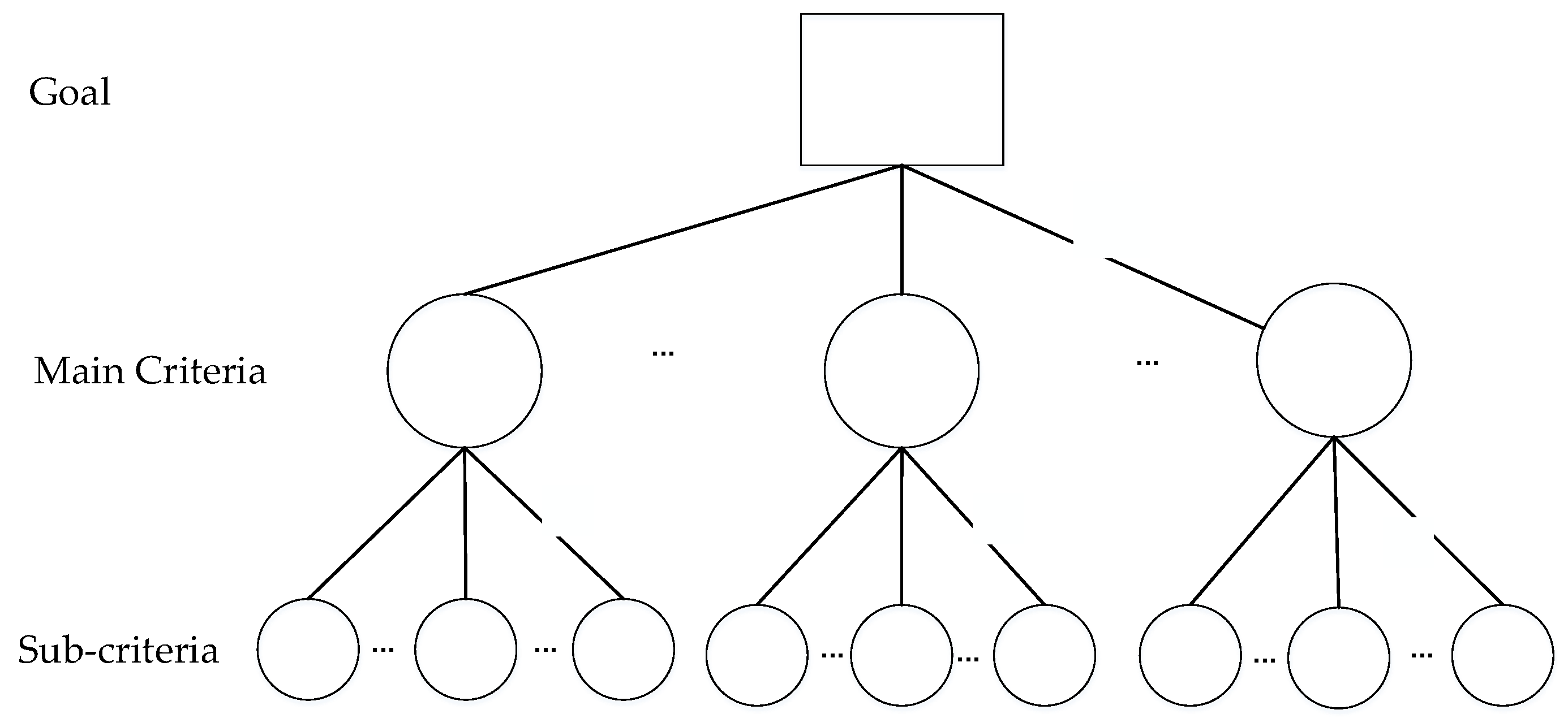
Let C I = { C 1 , C 2 , , C N } be a main criterion set, C i = { C 1 , C 2 , , C n } be a sub-criterion set. According the fuzzy AHP, a hierarchy structure should be built firstly. It contains the evaluation goal to be achieved at the top level, followed by the main criteria and sub-criteria to accomplish the goal, as shown in Figure 1. Upon forming the hierarchy, pairwise comparison judgments with TFNs can be obtained from selected experts’ judgments according to Chang [54], shown in Table 2. Let a I J k and a i j k represent the pairwise comparative judgments of expert k with TFNs at the main criteria layer and the sub-criteria layer, I , J = 1 , 2 , , N and i , j = 1 , 2 , , n . The following procedures are:
Step 1: Form individual fuzzy comparison matrices at each layer.
In order to understand relative importance of the criteria, the pairwise comparison judgments are aggregated as the individual fuzzy matrices with symmetric. Arithmetic rules should be complied in the following process: if i > j , a ˜ i j k is equal to the TFNs in Table 2. If i = j , a ˜ i j k is (1, 1, 1,). If i < j , a ˜ i j k is the reciprocal of these TFNs according to Equation (5). There is an example of an individual fuzzy comparison matrix W k given by expert k at the sub-criterion layer.
W k = | a ˜ 11 k a ˜ 12 k a ˜ 1 n k a ˜ 21 k a ˜ 22 k a ˜ 2 n k a ˜ n 1 k a ˜ n 2 k a ˜ n n k | n × n ,
Step 2: Check the consistency of individual comparison matrices.
The fuzzy elements in the individual matrices should be mapped to crisp BNP numbers using Equation (7) at first. Consistency ratio (CR) is introduced to test the consistency, as is:
C R = C I R I ,
where CI is a consistency index and RI is a random index. Let λmax be a largest eigenvalue of a fuzzy matrix, CI is
C I = λ max n n 1 ,
The RI values for different matrix orders are shown in Table 3. The lower the CR value is, the more consistent the matrix is. Experiential threshold 0.2 is usually recommended as the upper limit for CR of a fuzzy comparison matric [55]. If the CR value is less than 0.2, the matric is consistent approximately.
Step 3: Determine and transform fuzzy synthetic extent for each criterion.
In order to estimate the relative weights, the individual comparison matrices are aggregated according to an arithmetic average method. Let a ˜ I J and a ˜ i j be elements, the aggregated fuzzy comparison matrices at the main criteria layer ( W ¯ m ) and the sub-criteria layer ( W ¯ s ) are:
W ¯ m = ( a ˜ I J ) N × N ,
W ¯ s = ( a ˜ i j ) n × n ,
where a ˜ I J = 1 K k = 1 K a ˜ I J k and a ˜ i j = 1 K k = 1 K a ˜ i j k .
Let T I m = ( t I m L , t I m M , t I m R ) be the fuzzy synthetic extent at the main criteria layer, it is:
T I m = J N a ˜ I J N ,
where t I m L = J = 1 N a I J L N , t I m M = J = 1 N a I J M N , t I m L = J = 1 N a I J R N Similarly, the fuzzy synthetic extent T i s = ( t i s L , t i s M , t i s R ) at the sub-criteria layer is:
T i s = j n a ˜ i j n ,
where t i s L = j = 1 n a i j L n , t i s M = j = 1 n a i j M n , t i s L = j = 1 n a i j R n . In order to remove the fuzziness, T I m and T i s should be transformed into BNP values B I m and B i s .
Step 4: Compute normalized weights for all criteria
Consequently, the main criterion weight w I m and the sub-criterion local weight w i s can be obtained through normalization, as are:
w I m = B I m I = 1 N B I m ,
w i s = B i s i = 1 n B i s ,
According to the hierarchy structure, the normalized global weight w i s g for sub-criteria is:
w i s g = w I m × w i s ,

2.4.2. CRITIC Method for Objective Weights

Criteria Importance Through Intercriteria Correlation (CRITIC), proposed by Diakoulaki [56] in 1995, is a technique to determine objective weights of relative importance for criteria in many areas, such as engineering, economic, management and so on. The objective weights are derived based on contrast intensity and conflict in MCDM issues, which contain not only the criterion standard deviations among alternatives, but also the correlations of various criteria [57]. The method is suitable to be employed as an objective weighting decision technique in MCDM processes. Suppose that there are m alternatives and n criteria in a MCDM issue. Then an initial decision making matrix X is:
X = [ x i j ] m × n ,
Specially, for fuzzy MCDM problems, the decision making matrix containing fuzzy numbers should be transformed as BNP values based on Equation (7). Then the objective criteria weights can be obtained according to the following processes.
Step 1: Compute standard deviation σ j of each column vector x j to measure criterion contrast intensity among different alternatives, as is:
σ j = 1 m i = 1 m ( x i j x ¯ j ) 2 ,
where x ¯ j is the mean value of criterion j on all alternatives. The greater the σ j values are, the more obvious the divergence degree of the various alternatives.
Step 2: Determine the correlation coefficient r j k between different column vectors x j and x k to quantify the conflict resulted from criteria j and k. According to Pearson correlation coefficient, r j k is defined as:
r j k = i m ( x i j x ¯ j ) ( x i k x ¯ k ) i m ( x i j x ¯ j ) 2 × i m ( x i k x ¯ k ) 2 ,
It can be known that the more inconsistent the performances of criteria j and k, the lower the r j k value. Thus, the conflicting performance of criterion j associated with the rest is measured as:
k = 1 n ( 1 r j k ) ,
where the stronger positive correlations between criteria j and the others, the lower the conflicting performance.
Step 3: Integrate the contrast intensity and the conflicting performance to measure comprehensive decision information for each criterion through:
D j = σ j × k = 1 n ( 1 r j k ) ,
Step 4: Determine the normalized weights of all criteria by:
w j = D j j = 1 n D j ,

2.4.3. The Combination of Fuzzy AHP and CRITIC Weighting Methods

As mentioned above, subjective and objective mathematical techniques are introduced to determine criteria weights simultaneously. Let w j s be subjective weight determined by the fuzzy AHP and w j o be objective weight determined by the CRITIC method. The combination weight w ¯ j can be obtained in accordance with multiplicative synthesis, as is:
w ¯ j = w j s × w j o j = 1 n w j s × w j o ,

3. The Research Framework for the Hybrid MCDM Model

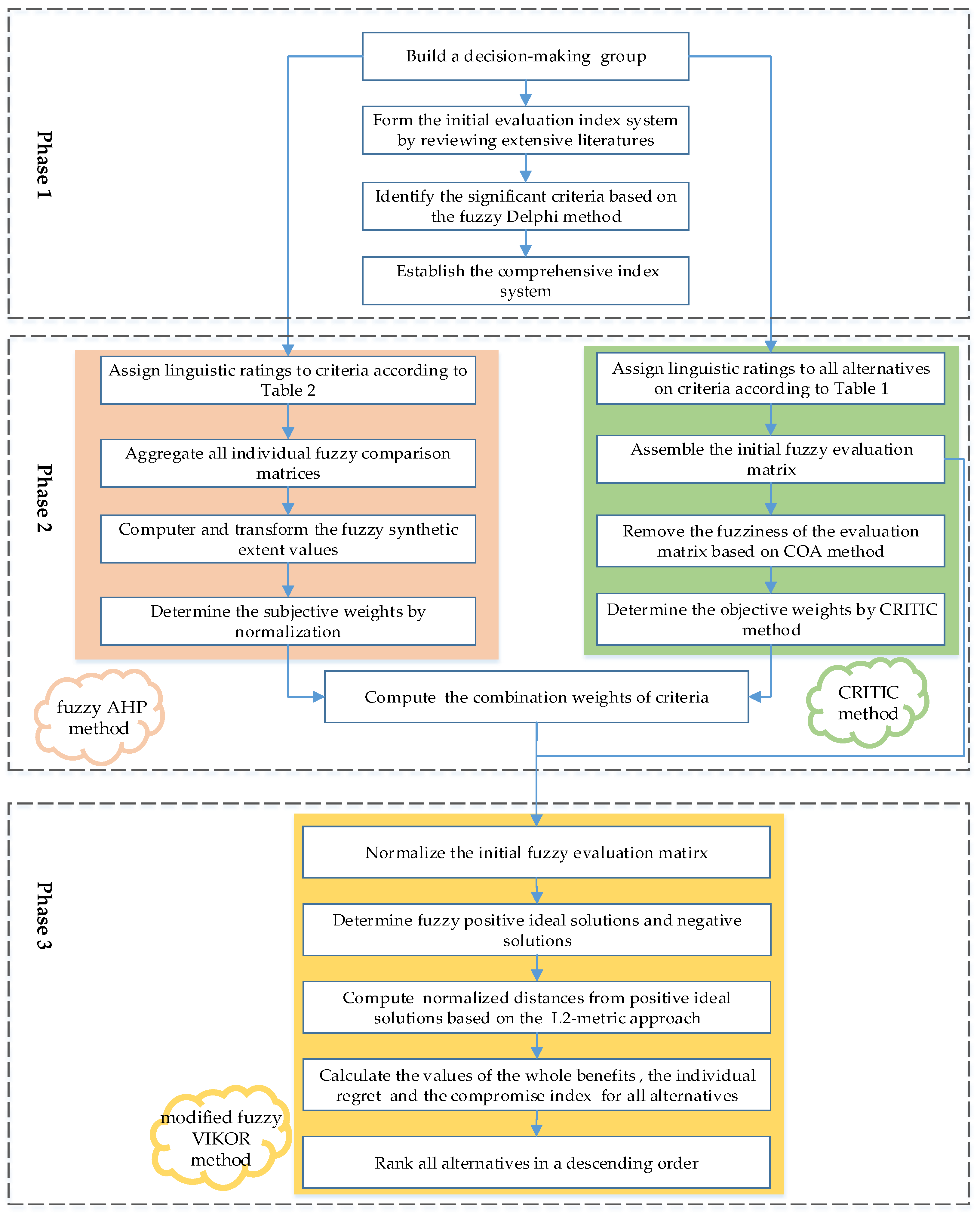
The integrated MCDM model is developed to evaluate the comprehensive performance of DR programs. Criteria weights are determined firstly by the combination weighting technique on the basis of fuzzy AHP and CRITIC methods. Then the alternative performances can be evaluated using the modified fuzzy VIKOR approach. The detailed evaluation procedures involve the following three phases, as shown in Figure 2.
Phase 1: Identify evaluation criteria to form a comprehensive index system based on the fuzzy Delphi method.
In the first phase, experts in the research fields of DR are invited to form a decision-making group. At the aim of descripting the performance of commercial DR from a comprehensive perspective, an initial index system is built by reviewing extensive literatures. Then, considering commercial DR features and experts’ opinions, significant criteria are selected to constitute a comprehensive evaluation index system by applying the fuzzy Delphi method. In addition, evaluation alternatives are confirmed.
Phase 2: Determine the aggregate weights of evaluation criteria based on fuzzy AHP and CRITIC methods.
At the basis of the comprehensive evaluation index system, the evaluation criteria are weighted by aggregating subjective weights and objective weights. For the subjective weights determined by the fuzzy AHP, relevant experts are asked to assign linguistic ratings to the evaluation criteria based on the linguistic variables (Table 2). Then, the consistencies of all individual comparison matrices are checked and all the matrices are aggregated. After computing and transforming the fuzzy synthetic extent values, the subjective weights can be obtained by normalization. For the objective weights determined by the CRITIC approach, vague linguistic ratings with respect to all alternatives on criteria are expressed by TFNs in Table 1. Then the initial fuzzy evaluation matrix is assembled and defuzzified through the COA method. The subjective weights can be determined by calculating the values of σ j , r j k and D j . On the basis of the above results, the aggregate weights for all criteria can be eventually obtained through multiplicative synthesis.
Phase 3: Assess comprehensive performance of the DR alternatives using the modified fuzzy VIKOR method.
In the last phase, the initial fuzzy evaluation matrix in the second phase is normalized firstly to eliminate the criterion dimension differences based on the linear scaling transformation method. Next, a series of fuzzy positive ideal solutions and negative solutions are determined. Then, the L2-metric approach is recommended to compute the normalized distances from positive ideal solutions. Finally, all evaluation results are calculated and all alternative performances are ranked in a descending order based on the values S i , R i and Q i .
The research framework of the proposed hybrid evaluation model based on the fuzzy Delphi, the combination weighting and the modified fuzzy VIKOR methods has the following four advantages in evaluating the comprehensive performance of DR. First, the application of the fuzzy logic theory may capture the fuzziness of human decision making. Second, employing the fuzzy Delphi method to select the evaluation criteria can reflect DR performance reasonably from multiple perspectives based on experts’ opinions. In addition, the combination weighting technique can integrate subjective and objective information to determine criteria weights, which also innovate the weighting determination process of conventional fuzzy VIKOR. Last, the modified fuzzy VIKOR is capable to efficiently handle vague decision making processes and the conflicting criteria existing in the performance evaluation. Therefore, the hybrid MCDM model is much more applicable to cope with real world issues.

4. A Comprehensive Evaluation Index System for DR Performances

4.1. The Initial Evaluation Index System

Evaluation criteria are particularly important to evaluate the performance of DR scientifically. For comprehensively reflect commercial DR inherent features, it is essential to build an initial evaluation index system. However, since DR programs are still in a primary stage of development in China, there are no unified criteria to evaluate the DR performance in the commercial sector. We try to establish an index system to evaluate the performance comprehensively from a sustainable perspective. Such programs are often applied to facilitate optimum allocation of energy resources as well as ensure reliable and economic operation of electrical power systems. According to the conventional sustainability theory, the initial index system should not only reflect short term economic benefits, but also include long term performance in social and environmental benefits [33]. Furthermore, considering complex technical conditions and management levels in the DR programs, some criteria from the two aspects should be much attention. Accordingly, the initial evaluation index system to comprehensively reveal the DR performance is proposed from five dimensions: economy, society, technology, environment and management. Further, relevant criteria are collected from some literatures and presented in Table 4.

4.2. The Final Evaluation Index System

Based on the research framework, final evaluation sub-criteria can be extracted from the initial index system by applying the fuzzy Delphi method. First of all, 50 experts from China are selected to form five advisory groups, which involves administrators, scholars, professors and project managers in the field of DR. Based on the current stable policy environment, incomplete electric power markets and imperfect energy trading mechanisms in China, they were asked to express opinions on sub-criteria significance as number intervals by e-mail. Then, the significance values of all initial sub-criteria were computed according to the fuzzy Delphi method procedures. In addition, the threshold value was recommended as 6 by most of the experts. Detailed calculation results are shown in Table 5. At last, the selected criteria marked with √ were aggregated to form the final evaluation index system, as shown in Figure 1.
The final evaluation index system for DR is established from a comprehensive perspective, which contains 5 main criteria and 16 sub-criteria. They are listed in the Figure 3.
(1) Economy criteria
The economy evaluation criteria of DR indicate various reductions of electric conduction investments and economic loss caused by power outages based on a perspective of power systems. Cost and profit criteria for specific DR programs are excluded. The main criterion includes 3 sub-criteria: reduced investments in new generation capacity and transmission and distribution equipment (J1), decreased loss of power transmission and transformation (J2), substantial operation cost reduction in power systems (J3), which are all benefit-type. All of these sub-criteria can effectively reflect DR performance from an economic aspect
(2) Society criteria
The society evaluation criteria focus on the role of DR programs in promoting social stability development, including electricity market construction, power supply reliability and sustainability. DR is considered as a powerful tool to improve the power industry transformation [27]. 3 sub-criteria are affiliated with the main criteria: mitigation of market power (J4), promotion of establishing more equitable and stable electricity prices (J5), avoidable outage in extreme reliability situations (J6). They can all attribute to benefit-type.
(3) Technology criteria
The technology evaluation criteria imply terminal equipment upgrades for DR programs. Because DR has been in an automation development stage, it is essential to apply new technologies as soon as possible [9]. Different technical levels may lead to different DR results. Smart meter coverage ratio (J7), establishment of large commercial HVAC systems (J8), flexible loads of each day on average (J9) constitute the technology criteria for commercial users, which are all benefit-type.
(4) Environment criteria
The environment evaluation criteria refer to pollution emission reduction and resource conservation caused by DR. Because of the DR role in decreasing peak loads and improving electric equipment utilization, a series of environmental advantages are prominent, including the mitigation of the reliance on fossil fuels (J10), increasing penetrations of renewable energy sources and distributed generation (J11), decreased GHG emissions (J12). They all belong to benefit-type.
(5) Management t criteria
The management evaluation criteria of DR performance refer to the internal management level of evaluation alternatives, which can be measured from the aspect of cost control, capital support and customer management. It includes the following sub-criteria: decreased electricity fee due to the decline in overall demand (J13), DR control equipment cost associated to each flexible kWh (J14), a reduction in service quality or productivity (J15) and capital adequacy for DR programs (J16). J14 and J15 are cost-type criteria, the rest are benefit-type criteria.

5. Empirical Analysis

5.1. Illustrate the Example

Shanghai is the first pilot city of DR implementation in China, which owns rich flexible resources and the potential to reduce peak loads. A series of DR programs have been carried out by load integrators and commercial building users to ease power shortages and ensure electric reliability. Therefore, at the aim of promoting the management level and the sustainable development of DR programs, the proposed framework can be applied to evaluate their performances. Building users are the focus of DR in Shanghai. We chose five commercial building users located in Pudong District as the empirical analysis objectives. Table 6 presents the characteristics of the five DR programs in the commercial buildings. In addition, they consume electricity from a coal-fired power plant with two 600 MW power capacity in Jiangsu Province.
The final evaluation index system is applied to rank the DR alternative performances. While four groups of decision-making experts familiar with DR were established to complete the linguistic ratings for criteria and alternatives. Table 7 shows the characteristics of the four expert groups. They responded to our research team's invitation by mail and participated in a communication meeting to finish a series of surveys.

5.2. Compute the Subjective Weights of Evaluation Criteria

Step 1: Assemble all individual fuzzy comparison matrices with respect to criteria importance.
Four groups of experts provided the importance of each criterion by using linguistic ratings and TFNs in Table 2. These TFNs can be assembled as a set of individual fuzzy comparison matrices based on a layer-by-layer analysis. Their consistencies should be confirmed by computing a series of CR values, as listed in Table 8. All CR values are below 0.2, which imply that all of the matrices are consistent and the judgments are credible.
Step 2: Obtain an initial fuzzy comparison matrix by aggregating these individual matrices.
Suppose A ˜ i j (i = 1,2…16, j = 1,2…16) be an element in an initial fuzzy comparison matrix. Take A ˜ 12 affiliated in economic main criteria as an example. The linguistic ratings from expert groups are MI, SI, SI and EI. It can be aggregated as:
A 12 L = 1 4 ( 1 + 3 2 + 3 2 + 1 2 ) = 1.13 ,
A 12 M = 1 4 ( 3 2 + 2 + 2 + 1 ) = 1.63 ,
A 12 R = 1 4 ( 2 + 5 2 + 5 2 + 3 2 ) = 2.13 ,
Thus, A ˜ 12 = ( 1.13 , 1.63 , 2.13 ) . Similarly, all initial fuzzy matrices in terms of criteria importance are obtained as shown in Table 9, Table 10, Table 11, Table 12, Table 13 and Table 14.
Step 3: Computer fuzzy synthetic extent values and determine the normalized subjective weights.
These fuzzy synthetic extent values T can be obtained under fuzzy environment by Equations (24)–(27), and then be mapped to BNP values. The subjective weights w i s g can be determined by normalization, which are shown in Table 15.

5.3. Compute the Objective Weights of Evaluation Criteria

Step 1: Establish the initial fuzzy evaluation matrix for alternatives.
After reviewing the performance and operation data of the five alternatives, the four groups of experts assigned the linguistic judgments to the evaluation criteria (Table 16) on the basis of Table 1.
Then the aggregated TFNs can be obtained to establish the initial fuzzy matrix. There is an example of aggregating the TFNs for alternative U1 with respect to sub-criteria J1.
x 11 L = 1 4 ( 3 + 1 + 3 + 5 ) = 3 ,
x 11 M = 1 4 ( 5 + 3 + 5 + 7 ) = 5 ,
x 11 R = 1 4 ( 7 + 5 + 7 + 9 ) = 7 ,
Thus, the aggregated TFN is x ˜ 11 = ( 3 , 5 , 7 ) . Similarly, the initial fuzzy evaluation matrix can be obtained by aggregating all TFNs, as shown in Table 17.
Step 2: Defuzzify the fuzzy numbers for the alternative performances.
Transform the aggregated TFNs in the initial fuzzy matrix to the BNP numbers according to the Equation (7), as show in Table 18.
Step 3: Calculate σ , r and D values for each criterion and normalized the objective weights.
The σ , r and D can be obtained using the Equations (32)–(36). The normalization of the objective weights w j o are computed. Detailed calculations are listed in Table 18.

5.4. Determine the Combination Weights of Evaluation Criteria

Integrating the merits of the fuzzy AHP and CRITIC methods, the combination weights of evaluation criteria can be obtained according to the multiplicative synthesis, shown in Table 19.

5.5. Evaluate the Comprehensive Performance of Alternatives

Step 1: Standardize the initial fuzzy evaluation matrix with linear scaling transformation method.
In order to ensure the compatibility of all criteria, the normalized fuzzy ratings of the five alternatives can be drawn based on Table 16, which are given as below:
J1(0.31,0.51,0.72)(0.62,0.82,0.97)(0,0.05,0.21)(0.67,0.87,1)(0.23,0.41,0.62)
J2(0.22,0.44,0.69)(0.5,0.75,1)(0.19,0.34,0.56)(0.44,0.69,0.94)(0.5,0.75,1)
J3(0.57,0.8,1)(0.23,0.46,0.69)(0.17,0.4,0.63)(0.2,0.4,0.63)(0.14,0.34,0.57)
J4(0.26,0.46,0.67)(0.72,0.90,1)(0.41,0.62,0.82)(0.67,0.85,0.95)(0,0.03,0.15)
J5(0.63,0.84,1)(0.21,0.42,0.63)(0.21,0.42,0.63)(0.32,0.53,0.74)(0.39,0.55,0.71)
J6(0.13,0.31,0.56)(0.52,0.76,1)(0.24,0.48,0.76)(0.45,0.69,0.97)(0.17,0.38,0.62)
J7(0.63,0.84,1)(0.47,0.68,0.89)(0,0.05,0.21)(0.42,0.63,0.84)(0.16,0.37,0.58)
J8(0.42,0.63,0.84)(0.63,0.84,1)(0.42,0.63,0.84)(0.68,0.87,1)(0.32,0.53,0.74)
J9(0.7,0.88,0.98)(0.8,0.9,1)(0.2,0.4,0.6)(0.7,0.85,0.98)(0.03,0.15,0.35)
J10(0.46,0.69,0.91)(0.56,0.78,0.97)(0.14,0.33,0.56)(0.67,0.86,1)(0.5,0.72,0.92)
J11(0.08,0.21,0.42)(0.63,0.84,1)(0.47,0.68,0.89)(0.53,0.74,0.92)(0.13,0.32,0.53)
J12(0.24,0.49,0.73)(0.55,0.79,1)(0.06,0.24,0.48)(0.55,0.79,1)(0.15,0.36,0.61)
J13(0.45,0.65,0.85)(0.75,0.9,1)(0.25,0.45,0.65)(0.75,0.9,1)(0.4,0.6,0.78)
J14(0.05,0.08,0.2)(0.03,0.04,0.05)(0.05,0.07,0.11)(0.03,0.03,0.05)(0.1,0.25,1)
J15(0.23,0.29,0.41)(0.23,0.29,0.44)(0.32,0.5,1)(0.23,0.29,0.44)(0.32,0.47,0.7)
J16(015,0.3,0.55)(0.8,0.9,1)(0.05,0.2,0.4)(0.6,0.75,0.88)(0.3,0.5,0.7)
Step 2: Determine the fuzzy positive ideal solutions and negative ideal solutions for all criteria
According to the Equations (14)–(15), the fuzzy positive ideal solutions z ˜ + and negative ideal solutions z ˜ with respect to all criteria can be determined, as shown in Table 20.
Step 3: Compute normalized distances from the positive idea solutions
Based on the L2-metric approach, the normalized distance of each alternative from the positive ideal solutions are calculated by Equation (16), respectively (Table 21).
Step 4: Calculate the values of S i , R i Q i and rank all alternatives
S i , R i and Q i values for all alternatives can be calculated by Equations (17)–(19) and sorted in a decreasing order, in which η = 0.5. They are shown in Table 22. Based on the conditions of “Acceptable advantage” and “Acceptable stability in decision making”, the final priority order is U2 > U4 > U3 > U1 > U5, shown in Table 23.

6. Findings and Discussions

We sorted the performances of the five DR programs by applying the combination weights and modified fuzzy VIKOR methods. Their ranking results in a descending order are U2, U4, U3, U1 and U5. The best alternative is U2 and the second one is U4. The above results imply that this proposed research framework can effectively evaluate and chose a best alternative to implement DR programs. Meanwhile, according to the Table 19, sub-criteria J4, J11 and J6 affiliated with society and environment main criteria get much more attention from expert groups, which reflect the goals and strategies of Chinese governmental apartments in electricity market construction and environmental protection. While the sub-criteria affiliated with economy and technology main criteria are not so important. As we all know, the electricity sector in China faces serious challenges from the “thirteen five-year” plan and an electricity market reform in 2015. The fact implies the target of the electricity industry for social responsibility and environment protection [60]. Competitive electricity market mechanisms are gradually being established to promote energy conservation and pollution reduction [61]. Therefore, the society and environment dimensions have been fully taken into account by experts for the DR performance evaluation in China.
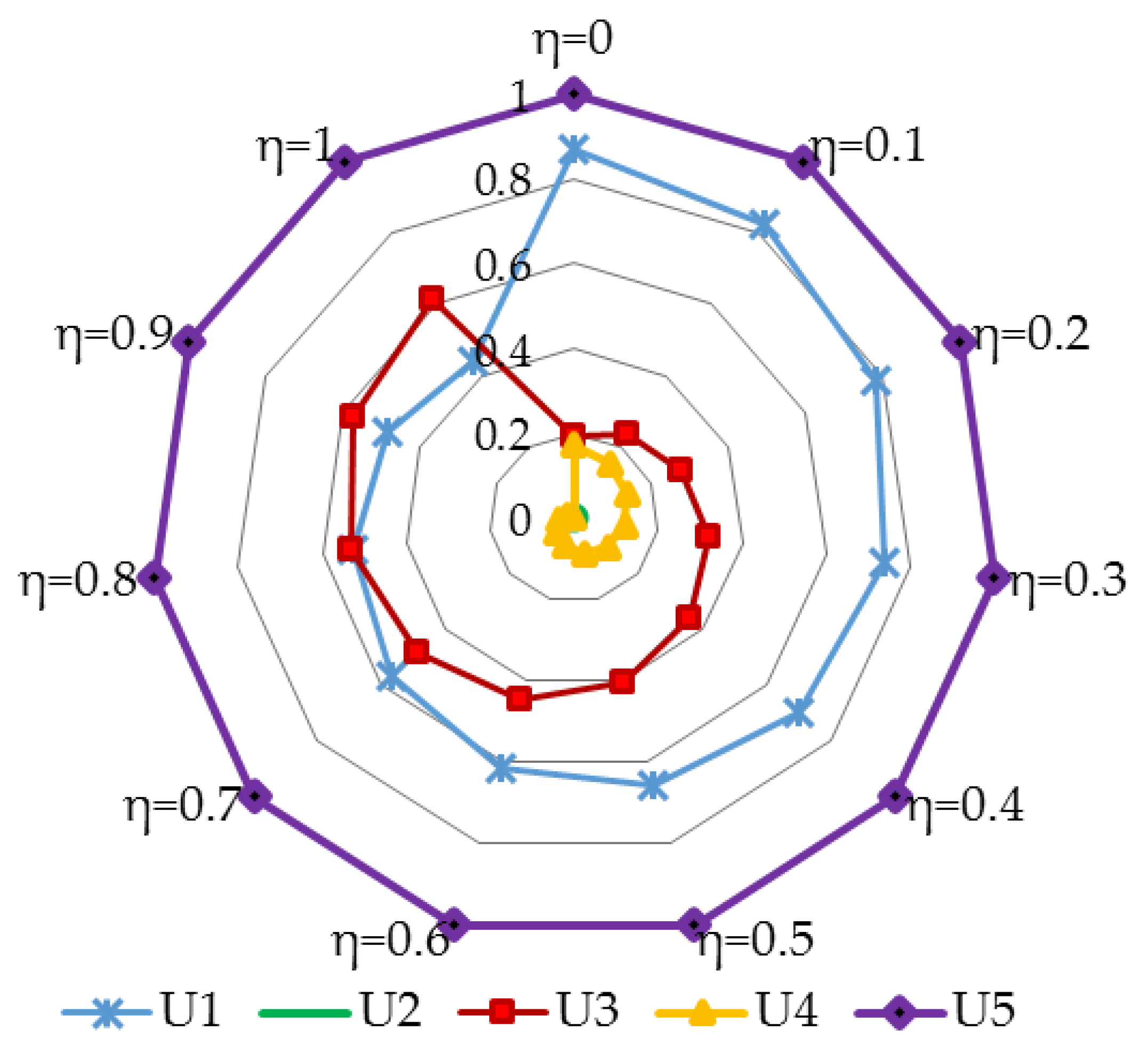
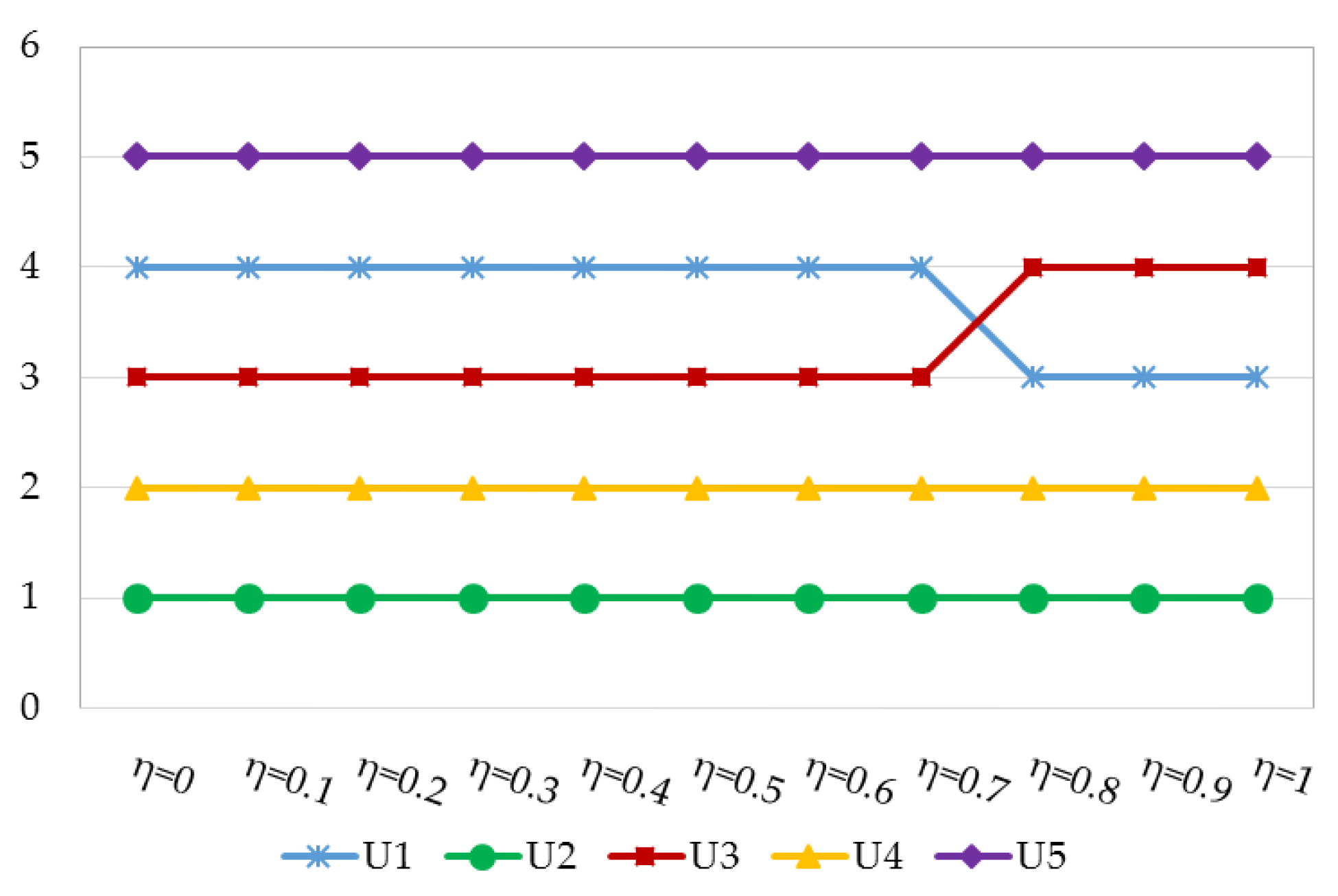
In order to validate the stability and rationality of the framework and research results, a series of sensitivity analyses for parameter η and criteria weights are conducted. First, the weight parameter for maximum overall benefits η is used from 0.0 to 1.0 increasing by 0.1 to reveal the impacts on final ranking results. The results are graphically presented in Figure 4. The final rankings of the five alternatives are shown in Figure 5. The best is still alternative U2, followed by U4. This study confirms that the ranking results determined by the proposed framework are effective and reliable.
Then a set of sensitive analyses on the impacts of criteria weights are conducted to obtain better insight of raking results and prove the robustness of these results. Sixteen sub-criteria affiliated in five main criteria have 20%, 40% and 60% more weight than the base weights and 20%, 40% and 60% less weight than the base weights. These base weights are presented in Table 19.
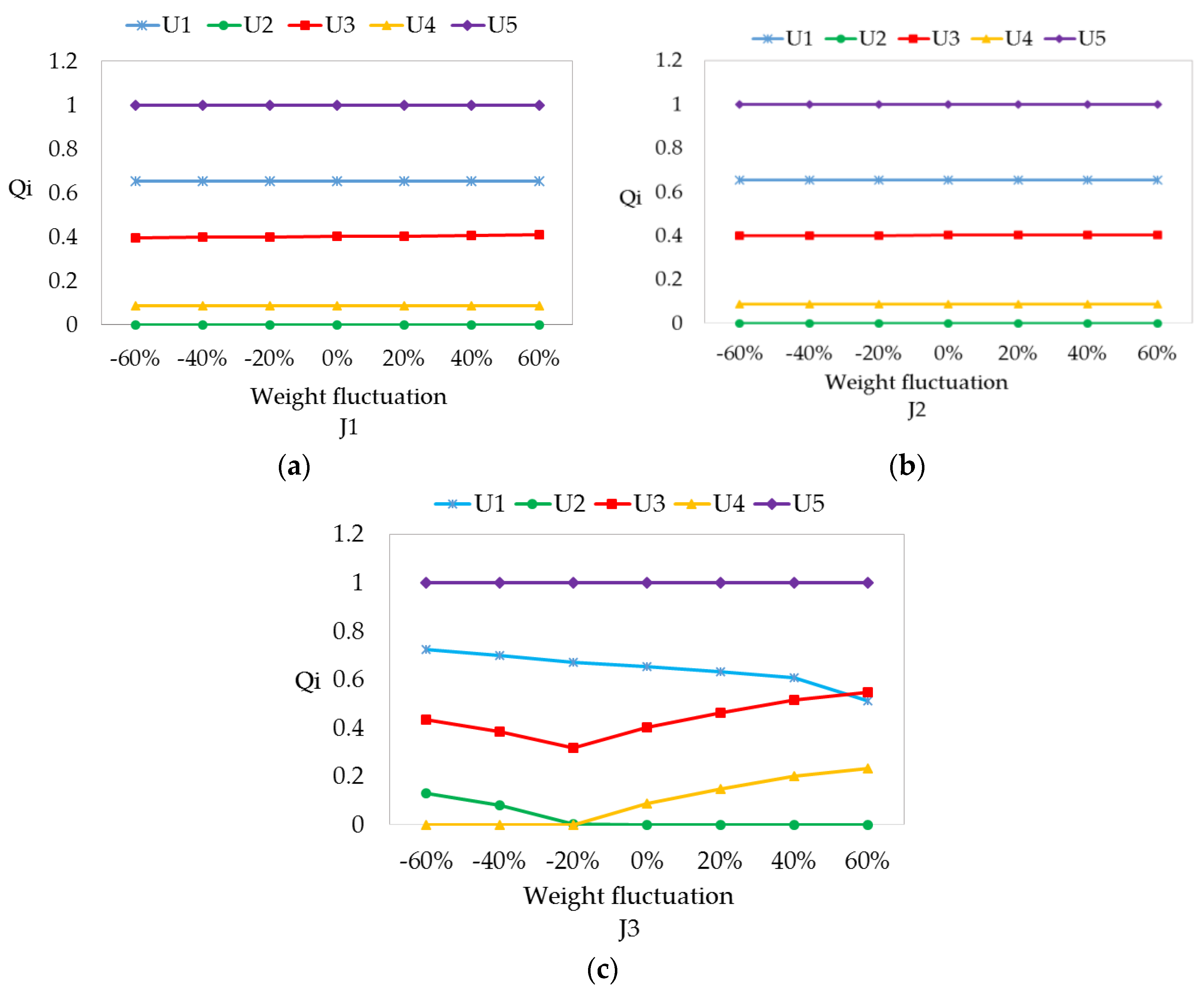
For the weight variations of sub-criteria in the economy main criterion, the Q i values of the five DR programs have small changes, no matter how the sub-criteria J1 and J2 change (Figure 6.). Moreover, as the weights of J3 decreases, the Q i values and rankings of U2 and U4 change obviously. It is seen that J3 is a sensible sub-criterion. However, no matter how the weight changes in the economy main criterion, U2 and U4 are still optimal alternatives.
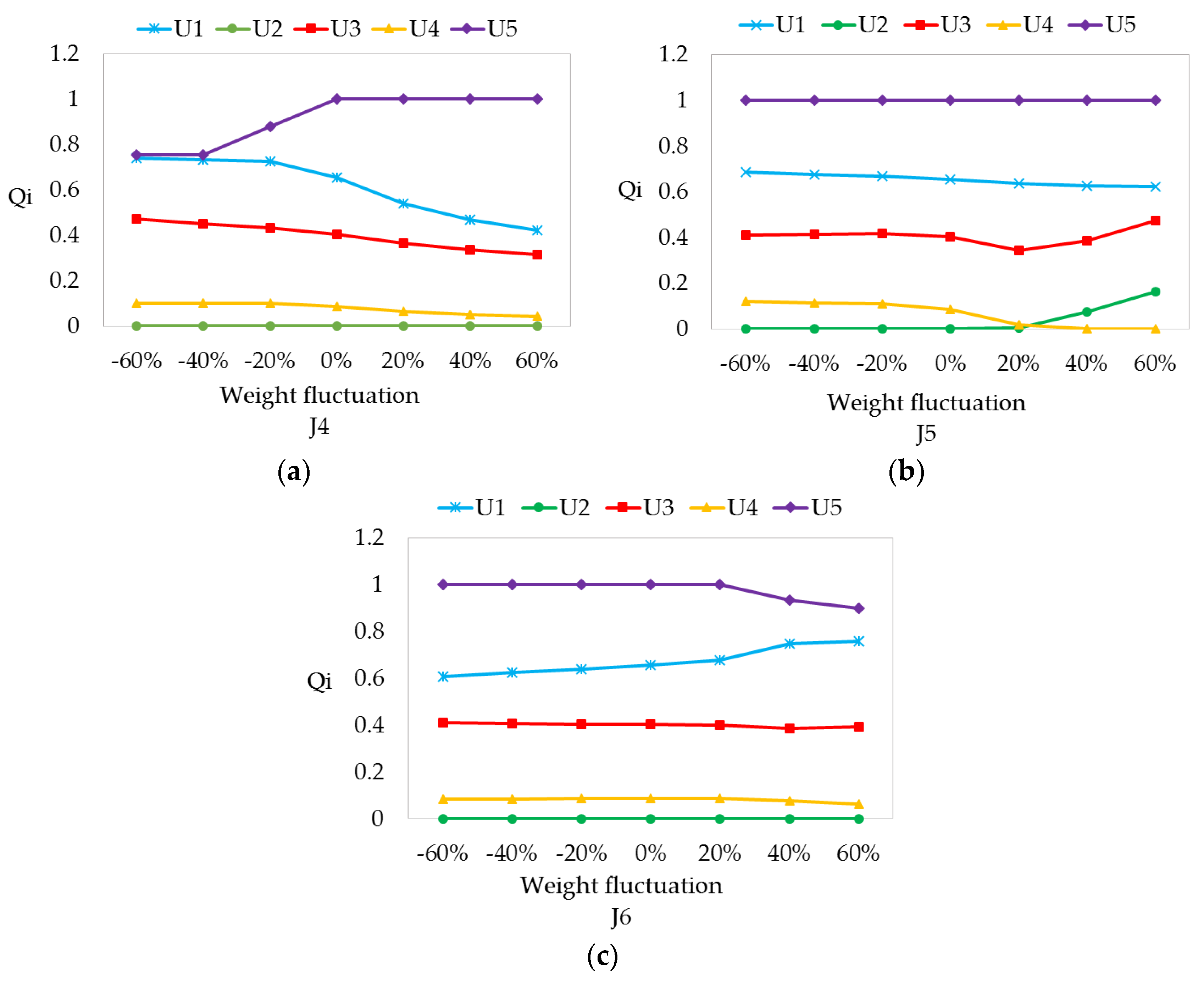
Figure 7 presents the cases of the sub-criteria weight fluctuations in the society main criterion. As J4 is more important, the Q i of U1, U3 and U4 are decreasing, while the value of U5 is increasing. With the increasing weight of J5, the Q i for U2, U3 and U4 are apparent variations and the sorting of U2 and U4 is inverted. Except for U2, the other values are changed in different degrees along with the weight fluctuation of J6. No matter how the sub-criteria weighs in the society main criterion change, U2 and U4 are priority choices. In addition, all the sub-criteria affiliated with the society main criterion are sensitive to weight fluctuations.
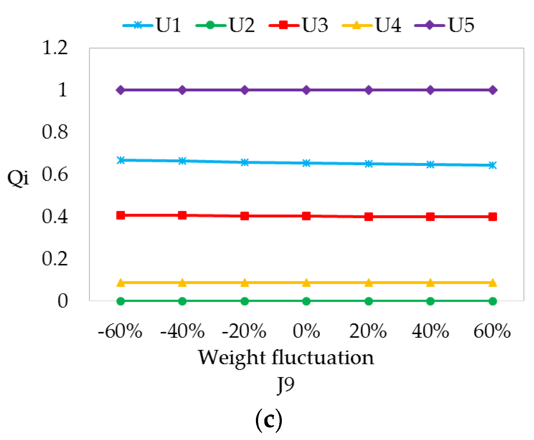
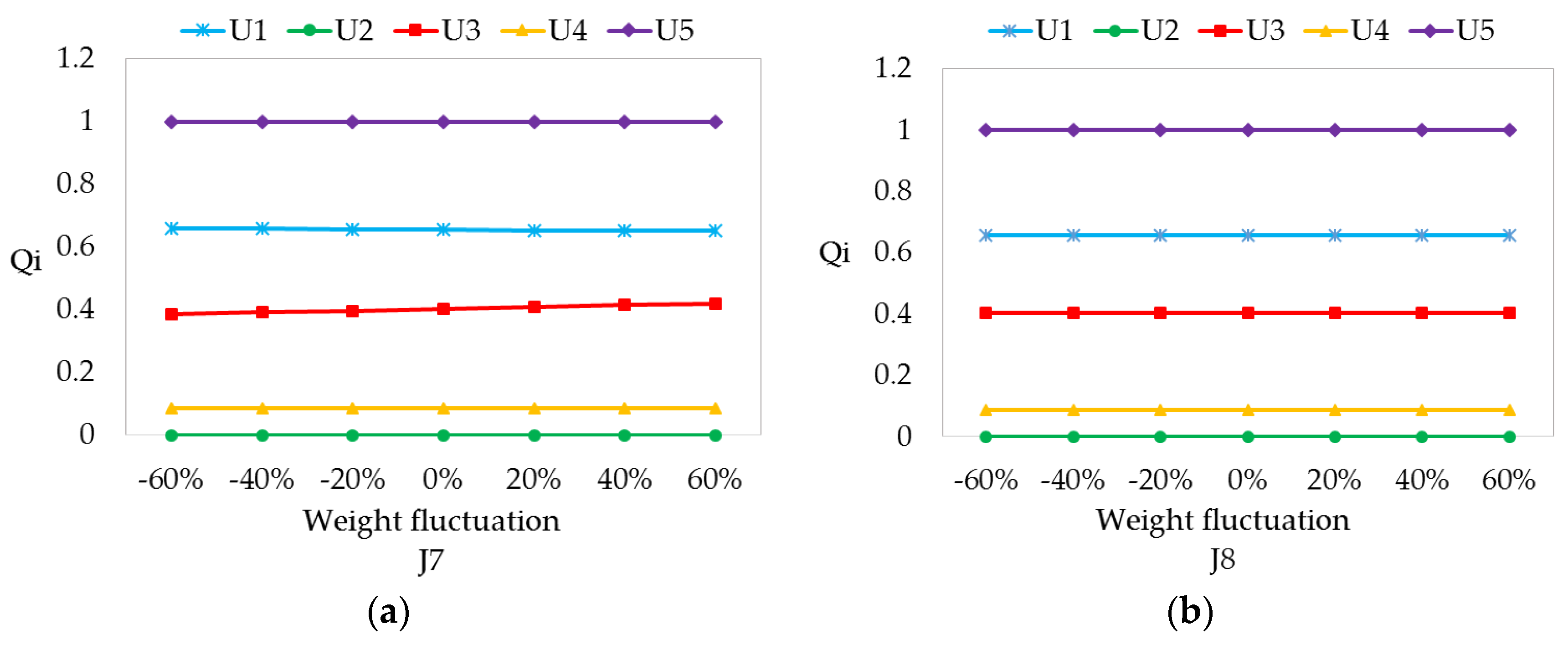
For the sub-criteria in the technology main criterion, the Q i of the five alternatives remain stable as the corresponding weights increase, which indicate that sub-criteria J7, J8 and J9 are stable (Figure 8).
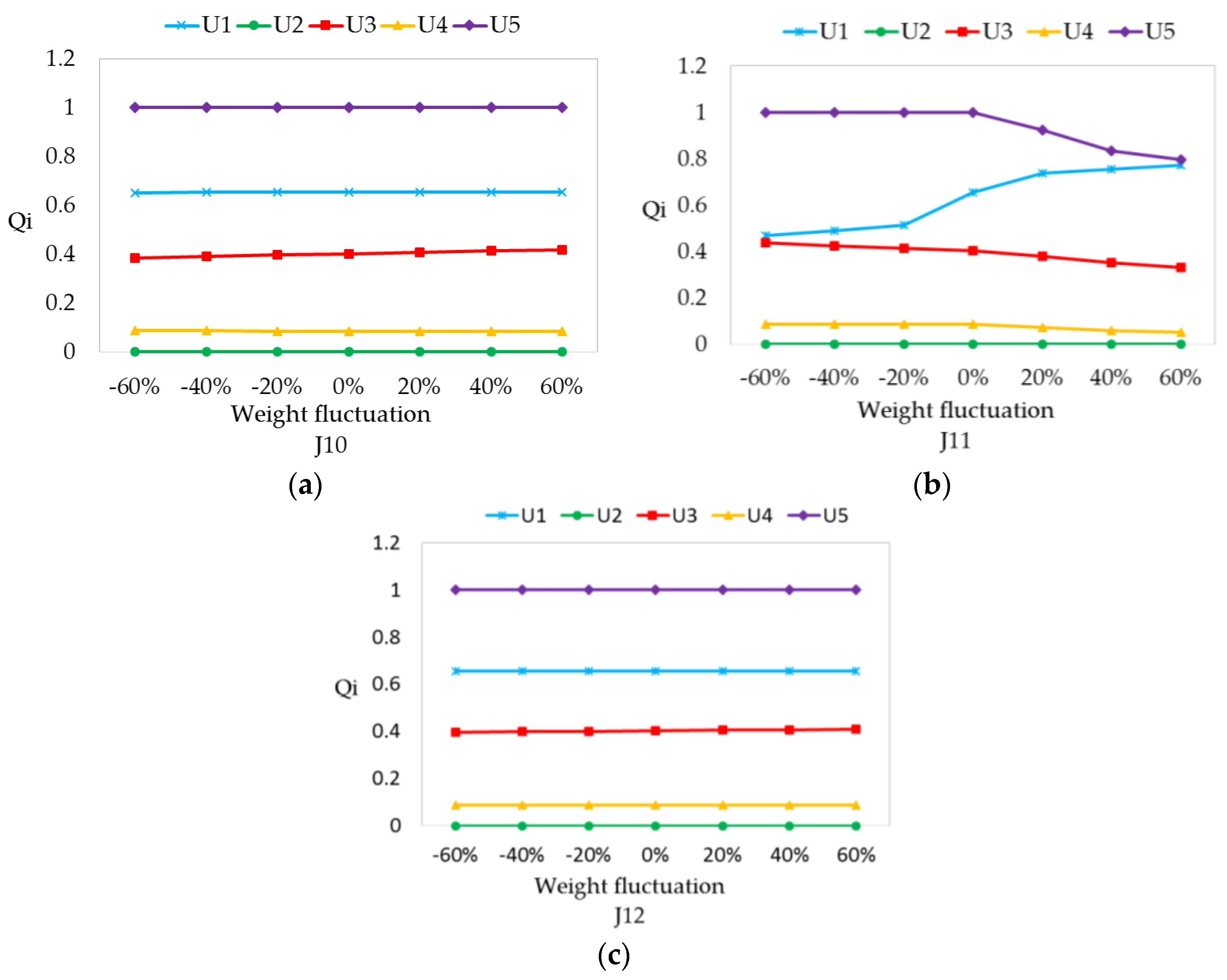
The cases in which the weights of three sub-criteria fluctuate in the environment main criteria are presented in Figure 9. As J10 and J12 are more important, the values Q i for all alternatives are tiny fluctuations. The Q i values have obvious variations along the weight of J11 increases. U1 and U5 get closer and closer significantly, which is similar to the trend of U2 and U4. However, no matter how the weights in the environment main criterion, U2 always keeps the supreme in the DR performance evaluation.
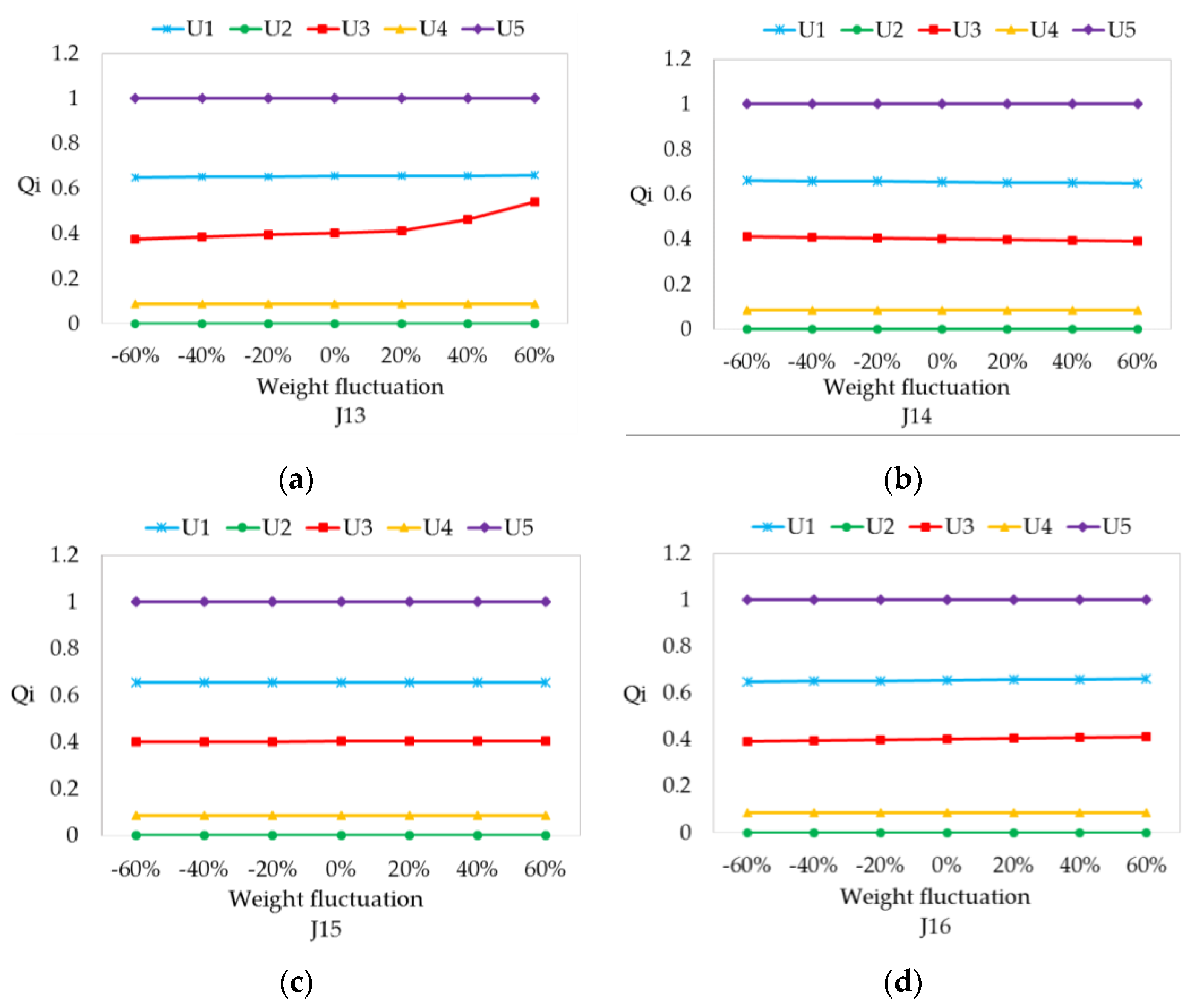
For the sub-criteria in the management main criterion, the Q i value of U3 presents an increasing trend along with J13 becomes more important (Figure 10). While in the cases of weight fluctuations of J14, J15 and J16, the Q i of the five alternatives hold a small variation trend. Just as that in the technology and environment main criteria, the final ranks of these five alternatives keep relatively stable, even though J13 carries a large weight in DR performance evaluation.
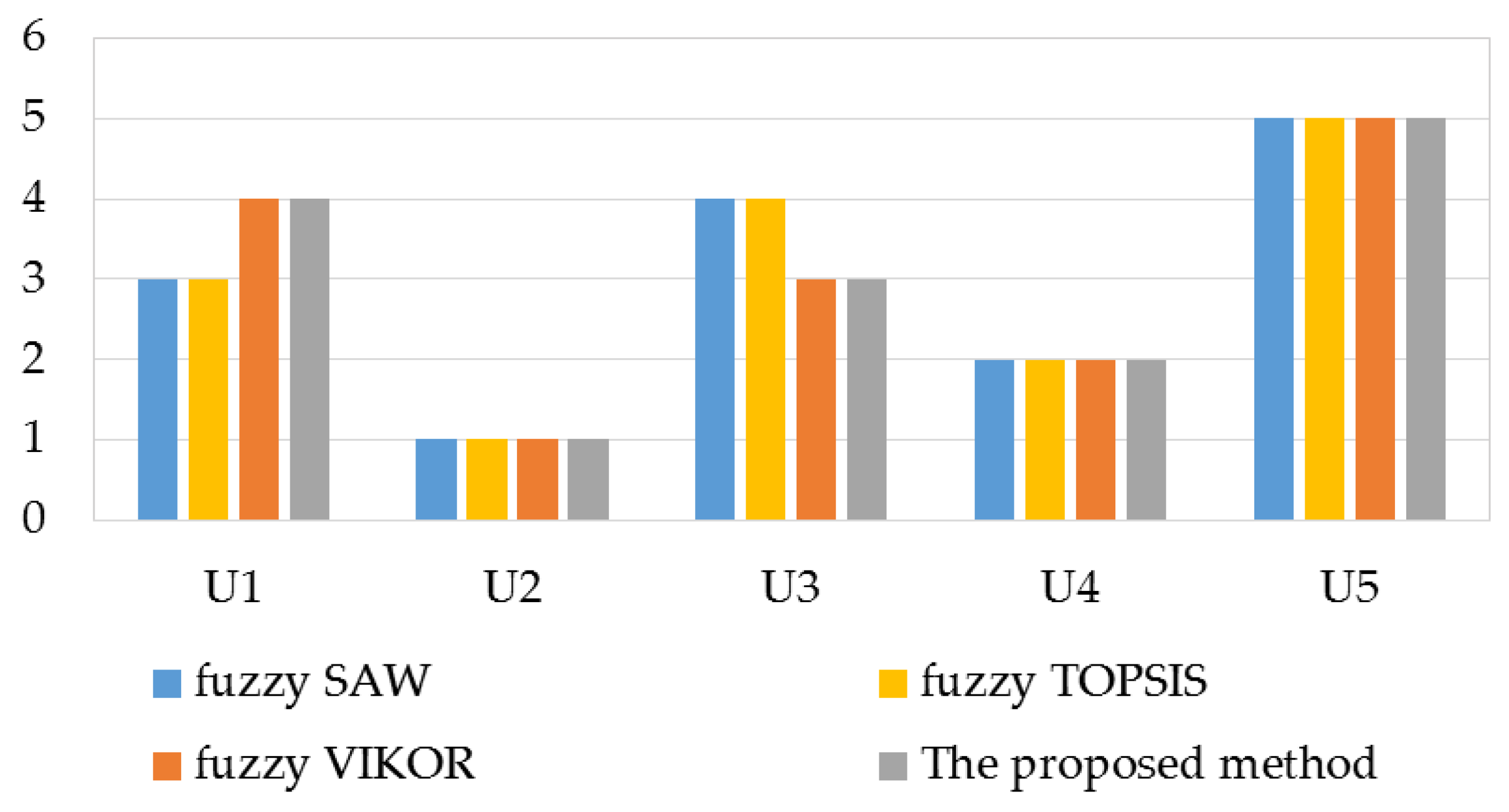
At the basis of the above analysis results, it is seen that the proposed method can effectively chose a best alternative. Moreover, to prove its validity, we applied the above cases to compare the results of the proposed method with the other comparable methods, including fuzzy simple additive weighting (SAW), fuzzy TOPSIS and previous fuzzy VIKOR methods. The fuzzy SAW approach, put forward by Chou [62], is to obtain a series of weighted sums of the performance ratings for all alternative. The fuzzy TOPSIS method, proposed by Chen [63], is that the selected alternative should present the shortest distance from the positive ideal values and the farthest distance from the negative ideal values. The previous fuzzy VIKOR method, developed by Kim [64], is used to find out compromise solutions based on differences of the fuzzy numbers rather than their precise distances. Here, the weights for the maximum overall benefits in the previous fuzzy VIKOR and the proposed method are set to 0.5. The linguistic ratings for all criteria performances listed in Table 16 and the base weights presented in Table 19 are uniformly applied to the four methods. Table 24 and Figure 11 show the analysis results. It is found that U2 and U4 are the best and the second choices in the three comparable approaches, which are consistent with the proposed method. The raking orders of the five alternatives using the fuzzy VIKOR and the proposed framework are the same.
Reference standards for criteria performances aren’t considered in the fuzzy SAW, which may result in an unconvincing ranking order. Although the fuzzy TOPSIS have contained the concept of ideal points, the weighting difference between positive and negative ideal values is ignored in the synthetic processes of each alternative performance. When an alternative is regarded as the top choice determined by the fuzzy TOPSIS, it does not mean that the alternative is always the closest to the ideal points. For the previous fuzzy VIKOR, the connection between alternatives and ideal points are defined as the uncertain differences between the corresponding TFNs, which have multiple feasible operations. For the proposed method, we introduced the precise L2-metric distances to determine the differences between alternatives and ideal points.

7. Conclusions

A hybrid framework for evaluating the performance of DR programs in the commercial sector was developed in this paper, which can efficiently promote the operation management of DR. In view of the sustainable development concept and commercial DR program features, an evaluation index system for performance evaluation of such programs was established, including five pillars: economy, society, technology, environment and management. The fuzzy Delphi method was recommended to select final evaluation criteria scientifically based on experts’ opinions. In order to cope with the fuzziness of human decisions and conflicts of evaluation criteria, the modified fuzzy VIKOR containing the L2-metric distance was applied to assess the comprehensive performance of the commercial DR. The method can not only grasp the vagueness in available information as well as the uncertainty of subjective judgments, but also solve the direct ranking of fuzzy numbers with respect of evaluation alternatives. In addition, in order to ensure a scientific weighting determination system, the evaluation weights were computed by integrating the subjective weights of the fuzzy AHP and the objective weights of the CRITIC, which replaced the weighting procedure of traditional fuzzy VIKOR. The hybrid framework with clear calculation processes was proven feasibly and effectively in the empirical study. The analysis results show that the sub-criteria J4, J11 and J6 affiliated with society and environment main criteria get much more attention from expert groups. To verify the robustness and effectiveness of evaluation results, a set of sensitivity analyses were performed, which presents that U2 and U4 always remain respectively the first and the second preferences along with criteria weight fluctuations and η value changes. Finally, a comparative study was conducted to demonstrate that our proposed framework can be used to determine the alternatives rankings and the priorities of improving criteria of weak alternatives.
There are still some limitations existing in the evaluation index system. Considering policy changes and electricity market development, we must timely update the evaluation criteria for commercial DR programs. The proposed framework will be performed again based on a new index system in order to track the DR evolutions. In our further study, we will test the proposed framework with other techniques from a methodological perspective. Moreover, the results from these techniques will be compared with the results in this paper to better overcome fuzziness in group decisions.

Acknowledgments

This study is supported by the Fundamental Research Funds for the Central Universities under Grant No. 2016XS68 and Energy Foundation No. G-1509-23762.

Author Contributions

Jun Dong and Huijuan Huo conceived and designed the research method framework; Dongran Liu performed the empirical analysis, Huijuan Huo and Rong Li analyzed the empirical results and wrote the paper.

Conflicts of Interest

The authors declare no conflict of interest.

References

  1. Zhao, X.; Luo, D. Driving force of rising renewable energy in China: Environment, regulation and employment. Renew. Sustain. Energy Rev. 2017, 68, 48–56. [Google Scholar] [CrossRef]
  2. Sun, W.; Meng, M.; He, Y.; Chang, H. CO2 Emissions from China’s Power Industry: Scenarios and policies for 13th Five-Year Plan. Energies 2016, 9, 825. [Google Scholar] [CrossRef]
  3. Thomaidis, N.S.; Santos-Alamillos, F.J.; Pozo-Vázquez, D.; Usaola-García, J. Optimal management of wind and solar energy resources. Comput. Oper. Res. 2016, 66, 284–291. [Google Scholar] [CrossRef]
  4. Ferruzzi, G.; Cervone, G.; Monache, L.D.; Graditi, G.; Jacobone, F. Optimal bidding in a day-ahead energy market for micro grid under uncertainty in renewable energy production. Energy 2016, 106, 194–202. [Google Scholar] [CrossRef]
  5. Siano, P. Demand response and smart grids—A survey. Renew. Sustain. Energy Rev. 2014, 30, 461–478. [Google Scholar] [CrossRef]
  6. Gellings, C.W. The Smart Grid: Enabling Energy Efficiency and Demand Response, Chapter 7; Taylor & Francis Group: Oxfordshire, UK, 2009; pp. 131–148. [Google Scholar]
  7. Pinson, P.; Madsen, H. Benefits and challenges of electrical demand response: A critical review. Renew. Sustain. Energy Rev. 2014, 39, 686–699. [Google Scholar]
  8. Goldman, C.; Hopper, N.; Bharvirkar, R.; Neenan, B.; Cappers, P. Estimating Demand Response Market Potential among Large Commercial and Industrial Customers: A Scoping Study; Lawrence Berkeley National Laboratory: Berkeley, CA, USA, 2007.
  9. Ferruzzi, G.; Graditi, G.; Rossi, F.; Russo, A. Optimal operation of a residential microgrid: The role of demand side management. Intell. Ind. Syst. 2015, 1, 61–82. [Google Scholar] [CrossRef]
  10. Paterakis, N.G.; Erdinç, O.; Catalão, J.P.S. An overview of Demand Response: Key-elements and international experience. Renew. Sustain. Energy Rev. 2017, 69, 871–891. [Google Scholar] [CrossRef]
  11. Cappers, P.; Goldman, C.; Kathan, D. Demand response in US electricity markets: Empirical evidence. Energy 2010, 35, 1526–1535. [Google Scholar] [CrossRef]
  12. Hu, Z.; Kim, J.; Wang, J.; Byrne, J. Review of dynamic pricing programs in the U.S. and Europe: Status quo and policy recommendations. Renew. Sustain. Energy Rev. 2015, 42, 743–751. [Google Scholar] [CrossRef]
  13. Torriti, J.; Hassan, M.G.; Leach, M. Demand response experience in Europe: Policies, programmes and implementation. Energy 2010, 35, 1575–1583. [Google Scholar] [CrossRef]
  14. Gils, H.C. Economic potential for future demand response in Germany-Modeling approach and case study. Appl. Energy 2016, 162, 401–415. [Google Scholar] [CrossRef] [Green Version]
  15. Campillo, J.; Dahlquist, E.; Wallin, F.; Vassileva, I. Is real-time electricity pricing suitable for residential users without demand-side management? Energy 2016, 109, 310–325. [Google Scholar] [CrossRef]
  16. Bradley, P.; Leach, M.; Torriti, J. A review of the costs and benefits of demand response for electricity in the UK. Energy Policy 2013, 52, 312–327. [Google Scholar] [CrossRef]
  17. Torriti, J. Price-based demand side management: Assessing the impacts of time-of-use tariffs on residential electricity demand and peak shifting in Northern Italy. Energy 2012, 44, 576–583. [Google Scholar] [CrossRef]
  18. Li, W.; Xu, P.; Lu, X.; Wang, H.; Pang, Z. Electricity demand response in China: Status, feasible market schemes and pilots. Energy 2016, 114, 981–994. [Google Scholar] [CrossRef]
  19. Yang, C.J. Opportunities and barriers to demand response in China. Resour. Conserv. Recycl. 2017, 121, 51–55. [Google Scholar] [CrossRef]
  20. Boßmann, T.; Eser, E.J. Model-based assessment of demand-response measures—A comprehensive literature review. Renew. Sustain. Energy Rev. 2016, 57, 1637–1656. [Google Scholar] [CrossRef]
  21. Qadrdan, M.; Cheng, M.; Wu, J.; Jenkins, N. Benefits of demand-side response in combined gas and electricity networks. Appl. Energy 2017, 192, 360–369. [Google Scholar] [CrossRef]
  22. Conchado, A.; Linares, P.; Lago, O.; Santamaría, A. An estimation of the economic and environmental benefits of a demand-response electricity program for Spain. Sustain. Prod. Consum. 2016, 8, 108–119. [Google Scholar] [CrossRef]
  23. FERC. Assessment of demand response and advanced metering. In Staff Report; Federal Energy Regulatory Commission: Wanshington, DC, USA, 2008. [Google Scholar]
  24. Klaassen, E.; Van Gerwen, R.; Frunt, J.; Slootweg, J. A methodology to assess demand response benefits from a system perspective: A Dutch case study. Util. Policy 2017, 44, 25–37. [Google Scholar] [CrossRef]
  25. Cepeda, M.; Saguan, M. Assessing long-term effects of demand response policies in wholesale electricity markets. Int. J. Electr. Power 2016, 74, 142–152. [Google Scholar] [CrossRef]
  26. Nolan, S.; O’Malley, M. Challenges and barriers to demand response deployment and evaluation. Appl. Energy 2015, 152, 1–10. [Google Scholar] [CrossRef]
  27. Siano, P.; Sarno, D. Assessing the benefits of residential demand response in a real time distribution energy market. Appl. Energy 2016, 161, 533–551. [Google Scholar] [CrossRef]
  28. Coughlin, K.; Piette, M.A.; Goldman, C.; Kiliccote, S. Estimating Demand Response Load Impacts: Evaluation of Baseline Load Models for Non-Residential Buildings in California; Lawrence Berkeley National Laboratory: Berkeley, CA, USA, 2008.
  29. Fera, M.; Macchiaroli, R.; Iannone, R.; Miranda, S.; Riemma, S. Economic evaluation model for the energy Demand Response. Energy 2016, 112, 457–468. [Google Scholar] [CrossRef]
  30. Karimi, E.; Kazerani, M. Impact of demand response management on improving social welfare of remote communities through integrating renewable energy resources. In Proceedings of the Electrical and Computer Engineering (CCECE), 2017 IEEE 30th Canadian Conference, Windsor, ON, Canada, 30 April 2017; pp. 1–6. [Google Scholar]
  31. Rodríguez-García, J.; Álvarez-Bel, C.; Carbonell-Carretero, J.-F.; Alcázar-Ortega, M.; Peñalvo-López, E. A novel tool for the evaluation and assessment of demand response activities in the industrial sector. Energy 2016, 113, 1136–1146. [Google Scholar] [CrossRef]
  32. Gils, H.C. Assessment of the theoretical demand response potential in Europe. Energy 2014, 67, 1–18. [Google Scholar] [CrossRef]
  33. Cobuloglu, H.I.; Büyüktahtakın, İ.E. A stochastic multi-criteria decision analysis for sustainable biomass crop selection. Expert Syst. Appl. 2015, 42, 6065–6074. [Google Scholar] [CrossRef]
  34. Bel, C.Á.; Ortega, M.A.; Escrivá, G.E.; Marín, A.G. Technical and economical tools to assess customer demand response in the commercial sector. Energy Convers. Manag. 2009, 50, 2605–2612. [Google Scholar]
  35. Safari, H.; Fagheyi, M.S.; Ahangari, S.S.; Fathi, M.R. Applying Promethee method based on entropy weight for supplier selection. Bus. Manag. Strategy 2012, 3, 97–106. [Google Scholar] [CrossRef]
  36. Zhang, S.; Sun, B.; Yan, L.; Wang, C. Risk identification on hydropower project using the IAHP and extension of TOPSIS methods under interval-valued fuzzy environment. Nat. Hazards 2013, 65, 359–373. [Google Scholar] [CrossRef]
  37. Daher, S.D.F.D.; de Almeida, A.T. Group preference aggregation based on ELECTRE methods for ERP system selection. In Enterprise Information Systems of the Future; Springer: Berlin/Heidelberg, Germany, 2013; pp. 215–222. [Google Scholar]
  38. Opricovic, S. Multicriteria optimization of civil engineering systems. Fac. Civ. Eng. Belgrad. 1998, 2, 5–21. [Google Scholar]
  39. Li, N.; Zhao, H. Performance evaluation of eco-industrial thermal power plants by using fuzzy GRA-VIKOR and combination weighting techniques. J. Clean. Prod. 2016, 135, 169–183. [Google Scholar] [CrossRef]
  40. San Cristóbal, J. Multi-criteria decision-making in the selection of a renewable energy project in spain: The Vikor method. Renew. Energy 2011, 36, 498–502. [Google Scholar] [CrossRef]
  41. Jahan, A.; Edwards, K. VIKOR method for material selection problems with interval numbers and target-based criteria. Mater. Des. 2013, 47, 759–765. [Google Scholar] [CrossRef]
  42. El-Wahed, W.F.A. Intelligent fuzzy multi criteria decision making: Review and analysis. In Fuzzy Multi-Criteria Decision Making: Theory and Applications with Recent Developments; Kahraman, C., Ed.; Springer Science & Business Media: Berlin/Heidelberg, Germany, 2008; Volume 16, pp. 19–37. [Google Scholar]
  43. Liao, H.; Xu, Z.; Zeng, X.J. Hesitant fuzzy linguistic VIKOR method and its application in qualitative multiple criteria decision making. IEEE Trans. Fuzzy Syst. 2015, 23, 1343–1355. [Google Scholar] [CrossRef]
  44. Safari, H.; Faraji, Z.; Majidian, S. Identifying and evaluating enterprise architecture risks using FMEA and fuzzy VIKOR. J. Intell. Manuf. 2016, 27, 475–486. [Google Scholar] [CrossRef]
  45. Zadeh, L.A. Fuzzy sets as a basis for a theory of possibility. Fuzzy Sets Syst. 1978, 1, 3–28. [Google Scholar] [CrossRef]
  46. Li, D.F. Compromise ratio method for fuzzy multi-attribute group decision making. Appl. Soft Comput. 2007, 7, 807–817. [Google Scholar] [CrossRef]
  47. Patel, A.V.; Mohan, B. Some numerical aspects of center of area defuzzification method. Fuzzy Sets Syst. 2002, 132, 401–409. [Google Scholar] [CrossRef]
  48. Dalkey, N.; Helmer, O. An experimental application of the Delphi method to the use of experts. Manag. Sci. 1963, 9, 458–467. [Google Scholar] [CrossRef]
  49. Murray, T.J.; Pipino, L.L.; van Gigch, J.P. A pilot study of fuzzy set modification of Delphi. Hum. Syst. Manag. 1985, 5, 76–80. [Google Scholar]
  50. Opricovic, S.; Tzeng, G.-H. Extended VIKOR method in comparison with outranking methods. Eur. J. Oper. Res. 2007, 178, 514–529. [Google Scholar] [CrossRef]
  51. Tiryaki, F.; Ahlatcioglu, M. Fuzzy stock selection using a new fuzzy ranking and weighting algorithm. Appl. Math. Comput. 2005, 170, 144–157. [Google Scholar] [CrossRef]
  52. Sanayei, A.; Mousavi, S.F.; Yazdankhah, A. Group decision making process for supplier selection with VIKOR under fuzzy environment. Expert Syst. Appl. 2010, 37, 24–30. [Google Scholar] [CrossRef]
  53. Saaty, T.L. What is the analytic hierarchy process? Math. Model. Decis. Support 1988, 48, 109–121. [Google Scholar]
  54. Chang, D.Y. Applications of the extent analysis method on fuzzy AHP. Eur. J. Oper. Res. 1996, 95, 649–655. [Google Scholar] [CrossRef]
  55. Junior, F.R.L.; Osiro, L.; Carpinetti, L.C.R. A comparison between Fuzzy AHP and Fuzzy TOPSIS methods to supplier selection. Appl. Soft Comput. 2014, 21, 194–209. [Google Scholar] [CrossRef]
  56. Diakoulaki, D.; Mavrotas, G.; Papayannakis, L. Determining objective weights in multiple criteria problems: The critic method. Comput. Oper. Res. 1995, 22, 763–770. [Google Scholar] [CrossRef]
  57. Wang, Y.M.; Luo, Y.; Wang, Y. Integration of correlations with standard deviations for determining attribute weights in multiple attribute decision making. Math. Comput. Model. 2010, 51, 1–12. [Google Scholar] [CrossRef]
  58. Hledik, R.; Faruqui, A. Valuing Demand Response: International Best Practices, Case Studies, and Applications. Available online: http://www.brattle.com/system/publications/pdfs/000/005/343/original/Valuing_Demand_Response__International_Best_Practices__Case_Studies__and_Applications.pdf?1468964700 (accessed on 26 July 2017).
  59. Juneja, S.; Black, J. Demand side response—A discussion paper. In Promoting Choice and Value for All Gas and Electricity Customers; Ofgem: London, UK, 2010. [Google Scholar]
  60. Zhou, K.; Yang, S. Demand side management in China: The context of China’s power industry reform. Renew. Sustain. Energy Rev. 2015, 47, 954–965. [Google Scholar] [CrossRef]
  61. Cherni, J.A.; Kentish, J. Renewable energy policy and electricity market reforms in China. Energy Policy 2007, 35, 3616–3629. [Google Scholar] [CrossRef]
  62. Chou, S.Y.; Chang, Y.H.; Shen, C.Y. A fuzzy simple additive weighting system under group decision-making for facility location selection with objective/subjective attributes. Eur. J. Oper. Res. 2008, 189, 132–145. [Google Scholar] [CrossRef]
  63. Chen, C.T. Extensions of the TOPSIS for group decision-making under fuzzy environment. Fuzzy Sets Syst. 2000, 114, 1–9. [Google Scholar] [CrossRef]
  64. Kim, Y.; Chung, E.S. Fuzzy VIKOR approach for assessing the vulnerability of the water supply to climate change and variability in South Korea. Appl. Math. Model. 2013, 37, 9419–9430. [Google Scholar] [CrossRef]
Figure 1. The hierarchical structure for the fuzzy analytic hierarchy process (AHP).
Sustainability 09 01332 g001
Figure 2. The research framework of the hybrid multiple criteria decision making (MCDM) model for evaluating demand response (DR) performance.
Sustainability 09 01332 g002
Figure 3. The final evaluation index system for DR performance in the commercial sector.
Sustainability 09 01332 g003
Figure 4. Sensitivity analysis results for different maximum overall benefits.
Sustainability 09 01332 g004
Figure 5. Alternative rankings for different maximum overall benefits.
Sustainability 09 01332 g005
Figure 6. Sensitivity analysis results of sub-criteria affiliated in economy main criterion.
Sustainability 09 01332 g006
Figure 7. Sensitivity analysis results of sub-criteria affiliated in society main criterion.
Sustainability 09 01332 g007
Figure 8. Sensitivity analysis results of sub-criteria affiliated with technology main criterion.
Sustainability 09 01332 g008aSustainability 09 01332 g008b
Figure 9. Sensitivity analysis results of sub-criteria affiliated in environment main criterion.
Sustainability 09 01332 g009
Figure 10. Sensitivity analysis results of sub-criteria affiliated in management main criterion.
Sustainability 09 01332 g010
Figure 11. The rankings of five alternatives using the four method.
Sustainability 09 01332 g011
Table 1. Linguistic variables for evaluating criteria performance [51].
Linguistic VariablesTFNs
Very poor (VP)(0,0,1)
Poor (P)(0,1,3)
Medium poor (MP)(1,3,5)
Fair (F)(3,5,7)
Medium good (MG)(5,7,9)
Good (G)(7,9,10)
Excellent (E)(9,10,10)
Table 2. Linguistic ratings and triangular fuzzy numbers (TFNs) for criterion weights.
Linguistic TermsTFNsMeaning
Equally important (EI)(1/2,1,3/2)Criteria i and j are equally important
Moderately important (MI)(1,3/2,2)Criterion i is moderately more important than j
Strongly important (SI)(3/2,2,5/2)Criterion i is strongly more important than j
Very strongly important (VI)(2,5/2,3)Criterion i is very strongly more important than j
Absolutely important (AI)(5/2,3,7/2)Criterion i is absolutely more important than j
Table 3. The values of RI.
n1,23456789101112131415
RI00.520.891.121.261.361.411.451.491.521.541.561.571.58
Table 4. An initial evaluation index system for DR performances.
Evaluation CriteriaLiteratures
Main CriteriaSub-Criteria
EconomyReduced investments in new generation capacity and transmission and distribution equipment[22,28]
Avoidable construction of new conventional power plants[22]
Decreased loss of power transmission and transformation[22,58]
Avoidable transmission and distribution network congestion due to overload[22,28,59]
Delay of power network upgrade and reinforcement[58]
Decreased capacity requirements of inefficient and expensive peaking power plants[28,58]
Substantial operation cost reduction in power systems[22,28]
Declining need for reserve and ancillary services[34,59]
Efficiency improvement of generating units in power systems[8]
SocietyImprovement of power system security and reliability[22,28]
Mitigation of market power[22]
Promotion of establishing equitable and stable electricity prices[22,58,59]
Enhancement of blackout restoration ability[58]
Avoidable outage in extreme reliability situations[58]
Weakening dependence on electricity import and export in neighboring areas[28]
Contribution to an incentive to consume electricity in an economical and effective manner[28,58]
TechnologySmart meter coverage ratio[48]
Capability of handling a large amount of data transfer[48]
Coverage ratio of energy efficiency equipment[34]
Satisfaction degree of technical standards for demand response[48]
Establishment of large commercial HVAC systems[22,48]
Flexible loads of each day on average[22,34]
EnvironmentThe mitigation of the reliance on fossil fuels[22]
Increasing penetrations of renewable energy sources and distributed generations[22,28]
Decreased greenhouse gas (GHG) emissions[28]
Decreased hazardous pollutant emissions in peak periods[58]
ManagementDecreased electricity fee due to the decline in overall demand[8,22]
DR control equipment cost associated to each flexible kWh[34]
Energy storage equipment cost related to each flexible kWh[34]
Metering and monitoring cost related to each flexible kWh[34]
Distributed energy system cost associated to each flexible kWh[59]
A reduction in service quality or productivity[34]
Prior experiences with load management projects[8]
Capital adequacy for DR programs[8]
Potential participation rate of power consumers[8]
Table 5. Calculation results of evaluation index based on the fuzzy Delphi method.
Main-CriteriaSub-CriteriaPessimistic TFNsOptimistic TFNs H i T i G i Results
EconomyReduced investments in new generation capacity and transmission and distribution equipment(6,7.33,9)(8,9.36,10)1.678.45
Avoidable construction of new conventional power plants(3,4.48,6)(5,6.52,8)2.525.50-
Decreased loss of power transmission and transformation(6,7.16,8)(8,9.17,10)2.848.17
Avoidable transmission and distribution network congestion due to overload(2,3.44,5)(5,5.55,7)3.564.50-
Delay of power network upgrade and reinforcement(3,4.13,5)(5,5.93,7)2.875.03-
Decreased capacity requirements of inefficient and expensive peaking power plants(3,4.04,6)(5,6.12,7)1.965.36-
Substantial operation cost reduction in power systems(6,6.78,8)(8,8,98,10)3.247.87
Declining need for reserve and ancillary services(3,3.57,4)(5,5.75,7)4.434.66-
Efficiency improvement of generating units in power systems(1,2.22,3)(4,4.74,6)4.783.48-
SocietyImprovement of power system security and reliability(1,2.05,3)(4,4.74,6)4.953.40-
Mitigation of market power(5,5.97,7)(7,8.16,9)3.037.07
Avoidable outage in extreme reliability situations(5,6.15,7)(7,7.95,9)2.857.05
Enhancement of blackout restoration ability(1,2.22,3)(4,5.14,6)4.783.68-
Promotion of establishing more equitable and stable electricity prices(5,6.15,7)(7,8.54,10)3.857.35
Weakening dependence on electricity import and export in neighboring areas(1,2.17,4)(3,4.79,7)3.833.49-
Contribution to an incentive to consume electricity in an economical and effective manner(2,2.93,4)(5,5.58,6)4.074.26-
TechnologySmart meter coverage ratio(4,5.14,6)(7,7.97,9)4.866.56
Capability of handling a large amount of data transfer(1,2.49,4)(4,5.14,6)3.513.82-
Coverage ratio of energy efficiency equipment(1,2.05,3)(4,4.54,6)4.953.30-
Satisfaction degree of technical standards for demand response(1,1.64,3)(3,4.28,6)4.362.96-
Establishment of large commercial HVAC systems(4,5.5,7)(6,7.35,8)1.56.47
Flexible loads of each day on average(5,5.75,7)(7,8.16,9)3.256.96
EnvironmentThe mitigation of the reliance on fossil fuels(5,5.75,7)(7,8.16,9)3.256.96
Increasing penetrations of renewable energy sources and distributed generations(4,5.14,6)(6,7.53,9)3.866.34
Decreased greenhouse gas (GHG) emissions(5,6.15,7)(7,8.36,9)2.857.26
Decreased hazardous pollutant emissions in peak periods(2,2.49,4)(4,4.92,6)3.513.71-
ManagementDecreased electricity fee due to the decline in overall demand(5,5.55,7)(7,8.16,9)3.456.86
DR control equipment cost associated to each flexible kWh(4,5.88,7)(7,8.72,10)4.127.30
Energy storage equipment cost related to each flexible kWh(1,1.64,3)(4,4.74,6)5.363.19-
Metering and monitoring cost related to each flexible kWh(2,3.25,5)(5,5.58,6)2.754.42-
Distributed energy system cost associated to each flexible kWh(1,2.17,4)(4,4.74,6)3.833.46-
A reduction in service quality or productivity(5,6.15,7)(7,8.16,9)2.857.16
Prior experiences with load management projects(1,2.46,5)(4,5.26,7)3.544.33-
Capital adequacy for DR programs(6,6.97,8)(8,9.17,10)3.038.07
Potential participation rate of power consumers(1,2.17,4)(3,4.48,6)2.833.45-
Table 6. The characteristics of the five DR programs in commercial buildings.
AlternativeU1U2U3U4U5
CategoryHotelShopping mallOfficeOfficeOffice
Built year19982005199420031989
Area (square meters)48,00063,00042,00057,00034,000
DR servicesHeating/Ventilation and air conditioningLighting/Ventilation and air conditioningLighting/Ventilation and air conditioningLighting/Ventilation and air conditioning/Information Communication and data transmissionLighting
DR operating year610585
Table 7. The characteristics of the four expert groups.
GenderAge RangeEducational LevelExperience (Year)Affiliation
MaleFemale
Expert group 1 (E1)3236–47Master or above≥5Government
Expert group 2 (E2)4138–56Doctor≥8Research institutions
Expert group 3 (E3)2328–41Master or above≥7Electricity utilities
Expert group 4 (E4)3232–44Bachelor or above≥5Building users
Table 8. Consistency ratio (CR) values of individual fuzzy comparative matrices for all the levels.
CRGoalO1O2O3O4O5
E10.0190.0090.0050.0110.0730.046
E20.1370.0520.0190.1810.0110.108
E30.0390.010.1810.1810.0050.141
E40.0450.010.0510.000.030.019
Table 9. The initial fuzzy comparison matrix of main criteria importance.
O1O2O3O4O5
O1(1,1,1)(0.60,0.83,1.17)(0.63,1.04,1.50)(0.53,0.81,1.10)(1.58,1.98,2.38)
O2(1,1.42,1.88)(1,1,1)(1,1.5,2)(1.06,1.35,1.67)(1.1,1.50,1.92)
O3(0.71,1.04,1.75)(0.52,0.71,1.17)(1,1,1)(1,1.33,1.75)(0.48,0.71,1.04)
O4(1.42,1.79,2.38)(1.06,1.35,1.67)(0.71,1.02,1.38)(1,1,1)(0.45,0.75,1.08)
O5(0.75,0.93,1.14)(0.71,0.93,1.25)(1.04,1.50,2.13)(1.08,1.50,2.25)(1,1,1)
Table 10. The initial fuzzy comparison matrix of sub-criteria importance affiliated in O1.
J1J2J3
J1(1,1,1)(1.13,1.63,2.13)(0.41,0.60,0.83)
J2(0.49,0.67,1.08)(1,1,1)(0.34,0.41,0.52)
J3(1.42,1.88,2.5)(2,2.5,3)(1,1,1)
Table 11. The initial fuzzy comparison matrix of sub-criteria importance affiliated in O2.
J4J5J6
J4(1,1,1)(1.13,1.63,2.13)(0.75,1.17,1.63)
J5(0.49,0.67,1.08)(1,1,1)(0.8,1,1.27)
J6(0.67,0.96,1.38)(1.33,1.73,2.13)(1,1,1)
Table 12. The initial fuzzy comparison matrix of sub-criteria importance affiliated in O3.
J7J8J9
J7(1,1,1)(1.63,2.13,2.63)(0.50,0.92,1.38)
J8(0.39,0.49,0.67)(1,1,1)(0.82,1.13,1.48)
J9(0.75,1.13,2)(1.13,1.48,2)(1,1,1)
Table 13. The initial fuzzy comparison matrix of sub-criteria importance affiliated in O4.
J10J11J12
J10(1,1,1)(0.6,0.92,1.29)(0.75,1.17,1.63)
J11(0.92,1.29,1.88)(1,1,1)(1.5,2,2.5)
J12(0.67,0.96,1.5)(0.43,0.58,0.92)(1,1,1)
Table 14. The initial fuzzy comparison matrix of sub-criteria importance affiliated in O5.
J13J14J15J16
J13(1,1,1)(0.88,1.38,1.88)(1.38,1.79,2.25)(1.25,1.67,2.13)
J14(0.56,0.79,1.42)(1,1,1)(0.73,1.13,1.54)(1.13,1.54,2)
J15(0.53,0.73,0.96)(0.79,1.08,1.63)(1,1,1)(0.43,0.56,0.79)
J16(0.56,0.77,1.04)(0.60,0.85,1.29)(1.38,1.88,2.38)(1,1,1)
Table 15. The fuzzy synthetic extent values and the weights of the evaluation criteria.
Main CriteriaSub-Criteria
T w I m T w i s w i s g
O1(0.06,0.28,0.91)0.137J1(0.15,0.33,0.59)0.1670.023
J2(0.06,0.09,0.19)0.0520.007
J3(0.94,1.56,2.5)0.7810.107
O2(0.23,0.86,2.4)0.380J4(0.28,0.63,1.15)0.4400.167
J5(0.13,0.22,0.46)0.1720.066
J6(0.3,0.55,0.97)0.3880.148
O3(0.03,0.14,0.74)0.100J7(0.27,0.65,1.2)0.4320.043
J8(0.11,0.18,0.33)0.1260.013
J9(0.28,0.55,1.33)0.4420.044
O4(0.1,0.37,1.18)0.179J10(0.15,0.36,0.7)0.2500.045
J11(0.46,0.86,1.56)0.5970.107
J12(0.1,0.18,0.46)0.1530.027
O5(0.12,0.39,1.36)0.204J13(0.38,1.03,2.24)0.5300.108
J14(0.11,0.34,1.09)0.2250.046
J15(0.05,0.11,0.31)0.0680.013
J16(0.12,0.31,0.8)0.1770.036
Table 16. Linguistic judgments for criteria performances of five alternatives.
J1J2J3J4J5J6J7J8J9J10J11J12J13J14J15J16
U1E1FPMGFGMPGFGFPFMGFGF
E2MPFFMPGPGFGMGPMPMGMPFMP
E3FMPGFMGPMGMGEFFMPFPPMP
E4MGFMGFMGFMGMGMGMGPFMGMPGMP
U2E1MGFFEMPFMGMGEFGFGMGMPG
E2GMGMPMGFMGMGMGGMGGMGGFGG
E3MGMGMPGFGFGGMGMGFEFFE
E4GFFGMPPMGGEGMGGGEMGE
U3E1VPFMPMGFFVPMGFFMGPFMPFMP
E2PPMPMGFFPMGFPMGPFVPPP
E3VPVPFFMPPVPFMPMPFMPMPMPMPMP
E4PFMPFMPMPPFMPMPMGMPFGFP
U4E1MGFFEFFMGMGEFGFGMGMPG
E2GMGMPFMGMGFMGGGFMGGMGGG
E3GFPGFMGMGEGEMGFEFFE
E4GFFGMPPFGMGMGMGGGEMGMP
U5E1MGFPVPFFMPFMPFFFGPMGF
E2PFMPVPGMPMPMPPFMPPMPVPMGMG
E3FMGMPPMGVPFMGPGMPMPMGVPVPMP
E4MPMGFVPVPMPMPFPMGPMPFMPFF
Table 17. The initial fuzzy evaluation matrix for alternatives based on the criteria performance.
U1U2U3U4U5
J1(3,5,7)(6,8,9.5)(0,0.5,2)(6.5,8.5,9.75)(2.25,4,6)
J2(1.75,3.5,5.5)(4,6,8)(1.5,2.75,4.5)(3.5,5.5,7.5)(4,6,8)
J3(5,7,8.75)(2,4,6)(1.5,3.5,5.5)(1.75,3.5,5.5)(1.25,3,5)
J4(2.5,4.5,6.5)(7,8.75,9.75)(4,6,8)(6.5,8.25,9.25)(0,0.25,1.5)
J5(6,8,9.5)(2,4,6)(2,4,6)(3,5,7)(3.75,5.25,6.75)
J6(1,2.5,4.5)(3.75,5.5,7.25)(1.75,3.5,5.5)(3.25,5,7)(1.25,2.75,4.5)
J7(6,8,9.5)(4.5,6.5,8.5)(0,0.5,2)(4,6,8)(1.5,3.5,5.5)
J8(4,6,8)(6,8,9.5)(4,6,8)(6.5,8.25,9.50)(3,5,7)
J9(7,8.75,9.75)(8,9,10)(2,4,6)(7,8.5,9.75)(0.25,1.5,3.5)
J10(4,6,8)(5,7,8.75)(1.25,3,5)(6,7.75,9)(4.5,6.5,8.25)
J11(0.75,2,4)(6,8,9.5)(4.5,6.5,8.5)(5,7,8.75)(1.25,3,5)
J12(2,4,6)(4.5,6.5,8.25)(0.5,2,4)(4.5,6.5,8.25)(1.25,3,5)
J13(4.5,6.5,8.5)(7.5,9,10)(2.5,4.5,6.5)(7.5,9,10)(4,6,7.75)
J14(1.25,3,5)(5,6.75,8.25)(2.25,3.75,5.25)(5.5,7.25,8.75)(0.25,1,2.5)
J15(4.25,6,7.5)(4,6,7.75)(1.75,3.5,5.5)(4,6,7.75)(2.5,3.75,5.5)
J16(1.5,3.5,5.5)(8,9,10)(0.5,2,4)(6,7.5,8.75)(3,5,7)
Table 18. BNP numbers and objective weights of the evaluation criteria based on Criteria Importance Through Intercriteria Correlation (CRITIC) method.
J1J2J3J4J5J6J7J8J9J10J11J12J13J14J15J16
U15.003.586.924.507.836.177.836.008.506.002.254.006.503.085.923.50
U27.836.004.008.504.0010.926.507.839.006.927.836.428.836.675.929.00
U30.832.923.506.004.007.830.836.004.003.086.502.174.503.753.582.17
U48.255.503.588.005.0010.336.008.088.427.586.926.428.837.175.927.42
U54.086.003.080.585.256.333.505.001.756.423.083.085.921.253.925.00
x ¯ j 5.204.804.225.525.328.324.936.586.336.005.324.426.924.385.055.42
( 1 r ) 4.829.6815.457.099.638.968.088.608.269.6413.157.097.545.736.665.31
σ 2.711.301.382.852.221.982.481.182.921.552.221.731.692.231.072.50
D 13.0312.5521.3320.2321.417.7620.0810.1824.114.9529.2112.2812.7812.777.113.29
w j o 0.050.0480.0810.0770.0810.0680.0760.0390.0910.0570.1110.0470.0490.0480.0270.05
Table 19. The Combination weights of evaluation criteria.
J1J2J3J4J5J6J7J8J9J10J11J12J13J14J15J16
w i s g 0.0230.0070.1070.1670.0660.1480.0430.0130.0440.0450.1070.0270.1080.0460.0130.036
w j o 0.0500.0480.0810.0770.0810.0680.0760.0390.0910.0570.1110.0470.0490.0480.0270.050
w ¯ j 0.0160.0050.1210.180.0740.140.0460.0070.0560.0360.1660.0180.0740.0310.0050.025
Table 20. The fuzzy positive ideal solutions and negative ideal solutions.
z ˜ + z ˜
J1(0.67,0.87,1)(0,0.05,0.21)
J2(0.5,0.75,1)(0.19,0.34,0.56)
J3(0.57,0.8,1)(0.14,0.34,0.57)
J4(0.72,0.9,1)(0,0.03,0.15)
J5(0.63,0.84,1)(0.21,0.42,0.63)
J6(0.52,0.76,1)(0.14,0.34,0.62)
J7(0.63,0.84,1)(0,0.05,0.21)
J8(0.68,0.87,1)(0.32,0.53,0.74)
J9(0.8,0.9,1)(0.03,0.15,0.35)
J10(0.67,0.86,1)(0.14,0.33,0.56)
J11(0.6320.84,1)(0.08,0.21,0.42)
J12(0.55,0.79,1)(0.06,0.24,0.48)
J13(0.75,0.9,1)(0.25,0.45,0.65)
J14(0.03,0.03,0.05)(0.1,0.25,1)
J15(0.23,0.29,0.41)(0.32,0.5,1)
J16(0.8,0.9,1)(0.05,0.2,0.4)
Table 21. Normalized distances of each alternative on criteria.
U1U2U3U4U5
J10.1920.004100.316
J20.598010.0250
J300.5710.780.7611
J40.25400.1040.0041
J50110.5560.465
J6100.4510.0260.862
J700.03910.070.37
J80.4730.0080.47301
J90.00400.4640.0061
J100.1340.026100.07
J11100.0610.0280.708
J120.3160100.609
J130.3070100.451
J140.03100.00801
J1500.00110.0010.405
J160.637010.0510.34
Table 22. The values of S i , R i and Q i for the five alternatives.
U1U2U3U4U5
Si0.4110.1460.5150.1470.747
Ri0.1660.0740.0940.0920.18
Qi0.65500.4030.0861
Table 23. The performance rankings of the five alternatives.
U1U2U3U4U5
Si31425
Ri41325
Qi41325
Table 24. The rating results of five alternatives using three methods.
Fuzzy SAWRankFuzzy TOPSISRankFuzzy VIKORRankProposed MethodRank
U10.52630.47930.25640.6554
U20.72310.82510101
U30.46840.37840.14930.4033
U40.68520.75820.09820.0862
U50.34950.15850.57515

