Measuring Efficiency and Effectiveness of Highway Management in Sustainability


1
Community Wellbeing Research Center, Graduate School of Public Administration, Seoul National University, Seoul 08826, Korea
2
Social Disaster & Safety Management Center, College of Liberal Arts, Korea University, Seoul 02841, Korea
*
Author to whom correspondence should be addressed.
Sustainability 2017, 9(8), 1347; https://doi.org/10.3390/su9081347
Submission received: 26 June 2017
/
Revised: 20 July 2017
/
Accepted: 21 July 2017
/
Published: 1 August 2017
(This article belongs to the Section Economic and Business Aspects of Sustainability)
Abstract
:This study analyses efficiency and effectiveness of highway management at the state level in the United States. While the current literature on highway management has contributed to understanding infrastructure budget and finance, the relationship between efficiency and effectiveness measurements has not been sufficiently discussed in the context of sustainability. To fill this gap, this study was systemically designed to test the relationship by controlling the states’ political factors, fiscal capacity, median voter, and economic conditions. Data envelopment and principal component analysis with panel data covering 11-year time waves were used to measure both efficiency and effectiveness. The results of the fixed effects model and the spatial autoregressive panel model show a statistically strong relationship between efficiency and effectiveness which are respectively measured by two analysis approaches.
1. Introduction
While the current literature on highway management has contributed to understanding infrastructure budget and finance, the relationship between efficiency and effectiveness measurements has not been sufficiently discussed in the context of sustainability. The purpose of this study was to empirically examine the relationship between efficiency and effectiveness of highway management in the field of sustainability.
Highway management has great consequences because public infrastructure management is closely connected to economic and social well-being and sustainability. Despite the significance, the topic, highway management, has not been spotlighted in the field of public budgeting and finance, compared with other budgeting issues [1]. So far, previous literature on infrastructure investment in the field of public affairs can be classified into two groups. One group deals with early studies that are about the normative approach of how to manage or improve capital assets [2,3,4]. For example, Millar [3] criticized that prior literature on capital budgeting is not useful for local governments to set capital project priorities. Rather, it was suggested that technical issues, organizational issues, and feasibility issues should form the criteria for setting priorities for capital projects. The other group is includes determinant studies of capital or infrastructure spending [5,6] and performance [7,8].
This study contributes to the discussion on sustainability management by focusing on highways as the target of empirical analyses. The study deals with efficiency and effectiveness that were discussed as performance proxies in prior literature and examines the empirical investigation between them. The importance of this study is summarized in its following contributions. First, the relationship between them has not been adequately discussed, though efficiency and effectiveness are the most important values in the public sector. Second, even though some studies deal with the relation between the two values [9,10,11], they do not provide empirical evidence on the relationship. Third, in terms of measuring efficiency, many studies for the public sector used efficiency as a dependent variable but employed just a fragmentary concept, such as a ratio of one input factor to one output factor. The concept of efficiency needs to be developed with the combination of multiple input and output factors. Fourth, the effectiveness of infrastructure management has been discussed mostly in the engineering field rather than in the field of sustainability management. Thus, the study aims to build up the concept of efficiency and effectiveness for infrastructure spending, to suggest measurement strategies, and to find empirical evidence on their relationship.
2. Theoretical Considerations
2.1. Sustainability and Highway Management
Sustainability is generally defined as “the capacity to maintain” [12]. In the field of highway management, suitability management is discussed with four aspects: environment, economy, financial management, and society [13]. U.S. Federal Highway Administration (FHWA) also presents three dimensions—environmental, economic, and social values—for the concept of the sustainable highway [14]. Similarly, the center for sustainable transportation defines a sustainable highway system as the one with safety, human and ecosystem health, and affordable costs, and one that is an environmentally friendly system [15].
A sustainable approach seeks to meet all of these needs while hitting economic targets for cost-effectiveness throughout a highway’s life cycle [14]. Again, a sustainable approach to highway management means helping stakeholders and decision makers reach balanced goals among environmental, socioeconomic, and public values—the triple bottom line of sustainability [13,14]—that will benefit current and future road users. This approach considers public access as more than just enhancing mobility and movement of people and goods, more than just managing vehicles and provision of transportation choices, e.g., optimized routes for walking, bicycling, and transit. That is, highway management in the field of sustainability includes various concepts including efficiency and effectiveness of funding, incentives for construction quality, regional air quality, resilience considerations, livability, and environmental management systems [14].
2.2. Concept of Efficiency
In the field of sustainability management, the definition of efficiency is well known and measured by the ratio of output to input. Similarly, the International Transport Forum [16] defines efficiency as “some combination of reduced costs and/or increased benefits to society (p. 89).” From this view, three specific definitions are explained: “reducing inputs for the same outputs; obtaining more outputs or improved quality for the same inputs; obtaining proportionally more outputs or improved quality in return for an increase in resources.”
However, the meaning of efficiency encompasses several concepts according to various perspectives, such as technical efficiency, allocative efficiency, and overall efficiency. Technical efficiency focuses on lower spending. It implies the maximum possible output at a given cost for a set of inputs in terms of output or, in cost terms, a certain level of output at the minimum possible cost [17,18]. Allocative efficiency is explained as “the right things are being done”; that is, the resources of a community should be allocated and used to maximize its welfare. More specifically, allocative efficiency is very close to Pareto efficiency, which means it is impossible to make a person better off without another person becoming worse off. “Another formal version of the same idea is to define an allocatively efficient level of production of a commodity as that level for which the difference between the ‘total social benefits’ from the consumption of the commodity and the ‘total social costs’ of its production is as large as possible’ [17] (p. 425).
Economists define allocative efficiency, technical efficiency, and overall efficiency by using geometrical and mathematical terms [19,20,21,22]. In Figure 1, the isoquants Ya and Yb indicate the same levels of output at different levels of input (A-D). First, the input mix for achieving allocative efficiency (AE) is defined as a set that minimizes production costs or a set that maximizes the level of output under “a fixed money outlay” [20] (p. 74). To compute the allocative efficiency (AE), the relative price of the input factor is required. In Figure 1, AE is measured as OD/OB and allocative inefficiency is 1 − OD/OB. Second, technical efficiency (TE) is defined as when an authority produces the same level of output with a lower level of input compared with others. Since the ability to create the difference in efficiency is regarded as a technique that can reduce the level of input, this efficiency is called technical efficiency. For example, in Figure 1, authority A uses a lower level of input than authority B; thus, authority A is appraised as technically more efficient than authority B, given the same levels of output (Ya and Yb). TE is OB/OA and inefficiency is measured as 1 − OB/OA. Third, overall efficiency is the product of AE and TE, which is defined as OD/OA (p. 75). In sum, allocative efficiency (AE) = OD/OB, technical efficiency (TE) = OB/OA, overall efficiency (OE) = AE * TE = OD/OA.
2.3. Concept of Effectiveness
Effectiveness is defined as a degree of goal achievement [23] (p. 149); however, many studies [24,25,26] discuss it as several aspects: goal attainment, system resource, reputation, and multi-dimensional model. First, in the goal attainment aspect, effectiveness is defined as the extent to which an organization achieves its goal, assuming goals that are stable, specific, objective, and able to be discovered [27] (p. 108). Second, the system resource approach regards effectiveness as “viability or survival,” which means the capacity of an organization to survive by obtaining or utilizing resources from environments [24,28]. Third, the reputation aspect sets forth effectiveness as a subjective opinion or perception on effectiveness. Opinions and perceptions are collected from individuals such as clients, staff, and other stakeholders familiar with the organization [24,25,26]. Lastly, the multi-dimensional aspects imply that effectiveness is measured by several components that can encompass aspects of goal attainment and system resource [24]. Cameron [29], citing his and his colleague’s prior research [30] said that a principal standard for effectiveness does not exist because the value is a combination of several preferences of individuals. Kushner and Poole [31] classified effectiveness into several types: constituent satisfaction, resource acquisition effectiveness, internal process effectiveness, goal attainment, and organizational effectiveness.
Based on the existing literature, this study employs the goal attainment approach. Since the study focuses on highway management and evaluates its performance, the system resource approach of organization capacity or the reputation model with subjective opinions do not fit with the study. Thus, multiple goals of highway policy are utilized for assessing effectiveness. For instance, Jimenez and Pagano [32] input several factors as drivers of effectiveness that were set using the Government Performance Project (GPP) data so as to set the proxy of capital management quality. They set GPP as a function of political variables (P), fiscal institutions (FI), state fiscal condition (FC), and environmental demand factors (E). Neshkova and Guo [7], who studied the citizen participation effect on highway expenditure efficiency and effectiveness, used two kinds of effectiveness indicators: road condition and fatality rate. They used citizen participation, task difficulty (e.g., public road length in miles, percentage of poor and mediocre conditioned road and bridges, and percent of miles traveled by trucks) and program resources (e.g., state owned source revenue on highway, federal aid in public transit, average payroll per employee, gasoline price, and motor fuel tax) as drivers of the two indicators.
2.4. Relation between Efficiency and Effectiveness
There are some studies encompassing contents on the relation between efficiency and effectiveness [9,10,11]. Peter Drucker insisted that efficiency is an inevitable consequence of effectiveness [9]. That is, effectiveness is prior to efficiency because the most important thing is to achieve what a government proposed to do rather than to work efficiently. Mandl, Dierx, and Ilzkovitz [10] explain the relationship between the two values by using the process of input-output-outcome (see Figure 2). The authors state, “effectiveness is more difficult to assess than efficiency, since the outcome is influenced political choice” (p. 3) which implies the impact of environmental factors is more crucial on effectiveness than on efficiency.
The 2 by 2 matrix of values depicted in Table 1 shows that some states achieve both effectiveness and efficiency together while some would have one of the two values or fail to attain either. For a government or an organization, the top priority is to achieve its goal, and the effectiveness is assessed by the extent to which a government’s outputs reach the goal. At the point when a government produces outputs for their goals with the least expenses, it is called an efficient government. For comparison, the best practice happens when the effectiveness accompanies the efficiency; the second best practice indicates when an organization achieves goals effectively but is less efficient than others; the third best practice means less effective but more efficient results, and the worst practice occurs when a government fails both values.
According to the theoretical literature and the conceptual framework, we assume efficiency and effectiveness are related. Prior studies present how to measure the two values, how the values are conceptualized in the process of input-output-outcome, and why effectiveness is prioritized over efficiency. However, few studies have empirically examined the relationship of the values. Thus, it is important and interesting to investigate whether and how efficiency and effectiveness are related.
3. Data, Methods, and Results
The study examines whether the two values, effectiveness and efficiency, are compatible and what the determinants of effectiveness are. The examination comprises a three-step process: (1) to measure efficiency; (2) to measure effectiveness with multiple quality factors; and (3) to examine whether the two values have a relation, controlling for other factors. For the purpose of the examination, we employ highway infrastructure cases. The unit of analysis is the state, and the analysis model is a spatial panel regression model. Thus, the data are obtained from the 48 adjoining U.S. states, excluding the non-contiguous states, Hawaii and Alaska, in order to use a spatial panel data model. Data cover 11 years (2000–2008 and 2012–2013). The data sources, Highway Statistics series, have some missing values at one point-in-time. For example, the 2009 data source does not have the information of “Estimated lane-miles” (HM-81) and “Weighted average daily traffic per lane” (HM-62). The data 2010 does not provide “Length by ownership” (HM-10), expenditure for highway (SF-12), pavement roughness (IRI, HM-64), and HM-62. SF-12 is missed in the 2011 data source. Highway Statistics, the Book of States, Comprehensive Annual Financial Reports (CAFR), National Association of State Budget Officers’ (NASBO’s) State Expenditure Report, and the U.S. census data are the sources of data.
3.1. Measuring Efficiency: Data Envelopment Analysis Approach
Banker, Janakiraman, and Natarajan [19] (pp. 14–28) distinguished concepts of productivity and efficiency. Following their explanation, we suppose two governments (A and B) who use x input and produce y output. The average productivities (AP) are defined as and for governments A and B, respectively. Higher AP means a higher level of productivity. Thus, the productivity index of government A is measured as . If П exceeds one, it means that government A is relatively more productive than the reference government. If we suppose that technology is known, then the maximum level of output is expressed as . Technical efficiency (TE) is measured as the ratio of actual output to “the maximum producible quantity,” and . In addition, the equation can be expressed as . This technical efficiency is output-oriented.
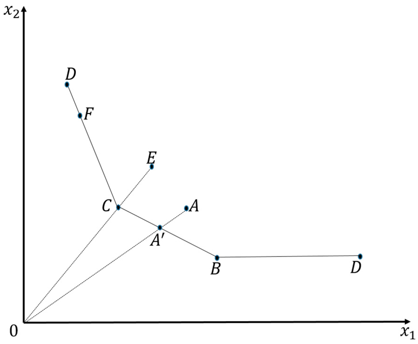
Data Envelopment Analysis (DEA) is useful for comparing the efficiency of each decision-making unit (DMU) [18,20,33]. Thus, DEA calculates the degree of efficiency of DMUs that produce the same kind of product, regarding the relative level of efficiency rather than an idealized standard of efficiency [18] (p. 471). As seen in Figure 3, which assumes one output with two inputs, five DMUs have efficient bundles of input among seven DMUs. Since the isoquant line envelops the inefficient DMUs A and E, it is called “data envelopment analysis” [20].
The basic function of DEA, according to Sherman and Zhu [34] (p. 64), is expressed as . The efficiency rating of the service unit is evaluated by DEA: y is amount of output, x is amount of input, i means number of inputs, r represents number of outputs, j indicates service unit, u is the coefficient or weight assigned by DEA to output r; and v is the coefficient or weight assigned by DEA to input i.
Data envelopment analysis was conducted to identify variations in the efficiency scores of 48 states. In the panel data of 11 years, we entered the length of lanes and the daily vehicle-miles traveled (DVMT) as output factors, and investment and maintenance expenditure of state highways were entered as input factors. Table 2 shows the information of data used in DEA.
Assuming constant return to scale and output-oriented DEA, the analysis yielded efficiency scores and their rankings. DEA efficiency scores are relative values among which the highest score is one. Table 3 presents a part of the DEA results, which has each state’s relative technical efficiency scores (TES) and its rankings. For example, in 2000, Georgia, Idaho, Ohio, and South Dakota are ranked first, but New Jersey is ranked the lowest. This efficiency score is more useful when comparing cases, whereas previous literature used the ratio of vehicle-miles to expenditures as an efficiency measure.
3.2. Measuring Effectiveness: Principal Component Analysis Approach
Based on the goal attainment approach, the study investigated goals of highway management. The American Association of State Highway and Transportation Officials (AASHTO), whose members are the officials of highway and transportation departments of 50 states, explains its goals as “development, operation, and maintenance” on their website [35]. The Office of Operations of the Federal Highway Administration (FHWA) mentions “transportation mobility, productivity, and safety” as its overall goals [36]. Referring to the aims of the federal agency and the association of state DOT (Department of Transportation) members, the study sets three goals of highway management: maintenance, mobility, and safety.
Measuring highway conditions acts as a proxy of maintenance. The Highway Statistics Reports have an international roughness index (IRI) and a present serviceability rating (PSR). The study adopts IRI because PSR is a subjective measure. The rule of thumb for interpretation of IRI is that values less than 95 indicate a good condition of road roughness and values less than 170 mean an acceptable condition. Therefore, higher values represent worse road conditions. Qiu [37] used safety and mobility as highway maintenance performance elements. Safety can be measured by “persons fatally injured in motor vehicle crashes” per 100 million vehicle-miles traveled. In addition, mobility can be shown by annual average daily traffic and volume-to-service flow ratio.
In terms of measuring effectiveness, we employ a factor analysis method. Previous studies normally adopted factor analysis to create effectiveness indicators [23,30]. To estimate the effectiveness indicator, we first estimate factor scores using the principal component analysis (PCA) and then apply a variance value as a weight for each component. Thus, the total value of effectiveness is computed as the summation of each state’s product of weights and factor scores:
where i means each state, W is a weight, m indicates each component, and F means a factor score.
To find the effectiveness indicator, we employ road condition (IRI), fatality (the number of people fatally injured), and congestion (the annual average daily traffic: AADT). First, we recode raw data values to establish a consistent direction for each variable’s value. IRI has score ranges of “<60, 60–94, 95–170, 171–220, and >220,” and a higher value of IRI means poorer quality. We divided the ranges into “good (IRI < 95),” “fair (95 ≤ IRI ≤ 170),” and “unacceptable (IRI > 170)” according to the literature [38,39,40] and coded them as 3, 2, and 1, respectively. Then, we computed the weighted mean of each state highway by using the ratio of the certain quality road miles to the total miles: . Fatality and congestion are calculated as the reciprocal of the number of people fatally injured over lane-mile and the reciprocal of AADT per lane-mile and renamed as safety and mobility respectively. Thus, the recoded factors (road condition, safety, and mobility) indicate that a higher value means a better performance. Table 4 has the detailed data information of each component for measuring effectiveness indicator.
Second, running the principal component analysis, we found one main component and its factor score. I employed the component’s percentage points of variance as a weight value. Thus, the effectiveness indicator is calculated as the product of the factor score and weights value:
Table 5 presents states’ effectiveness indicators, road conditions, safety, and mobility in 2000, 2005, and 2012. For instance, in 2012, West Virginia was the most effective in highway management, but New Jersey was ranked the lowest. With respect to road conditions, Georgia was the best at highway maintenance, but Rhode Island was the worst. West Virginia was ranked first in safety and mobility, but New Jersey and California were the lowest.
3.3. Modeling Relationship between Efficiency and Effectiveness
3.3.1. Data and Unit of Analysis
To conduct regression analysis, we collected data regarding state highway management. Highway data came from the highway statistics series by the U.S. Federal Highway Administration. Financial data are available from the U.S. Census Bureau. We also used data from the National Conference of State Legislatures (NCSL) and the National Association of State Budget Officers (NASBO).
We pooled data for 48 U.S. states from 2000 to 2013, except 2009 to 2011. Consequently, Alaska and Hawaii were dropped from the analysis because the study analyzes only contiguous states, considering the geographical effect by using a spatial regression model. Our data also do not include 2009–2011 data because of missing information on capital outlay and maintenance, the length of lanes, and DVMT, as explained in Table 2.
3.3.2. Dependent and Explanatory Variables
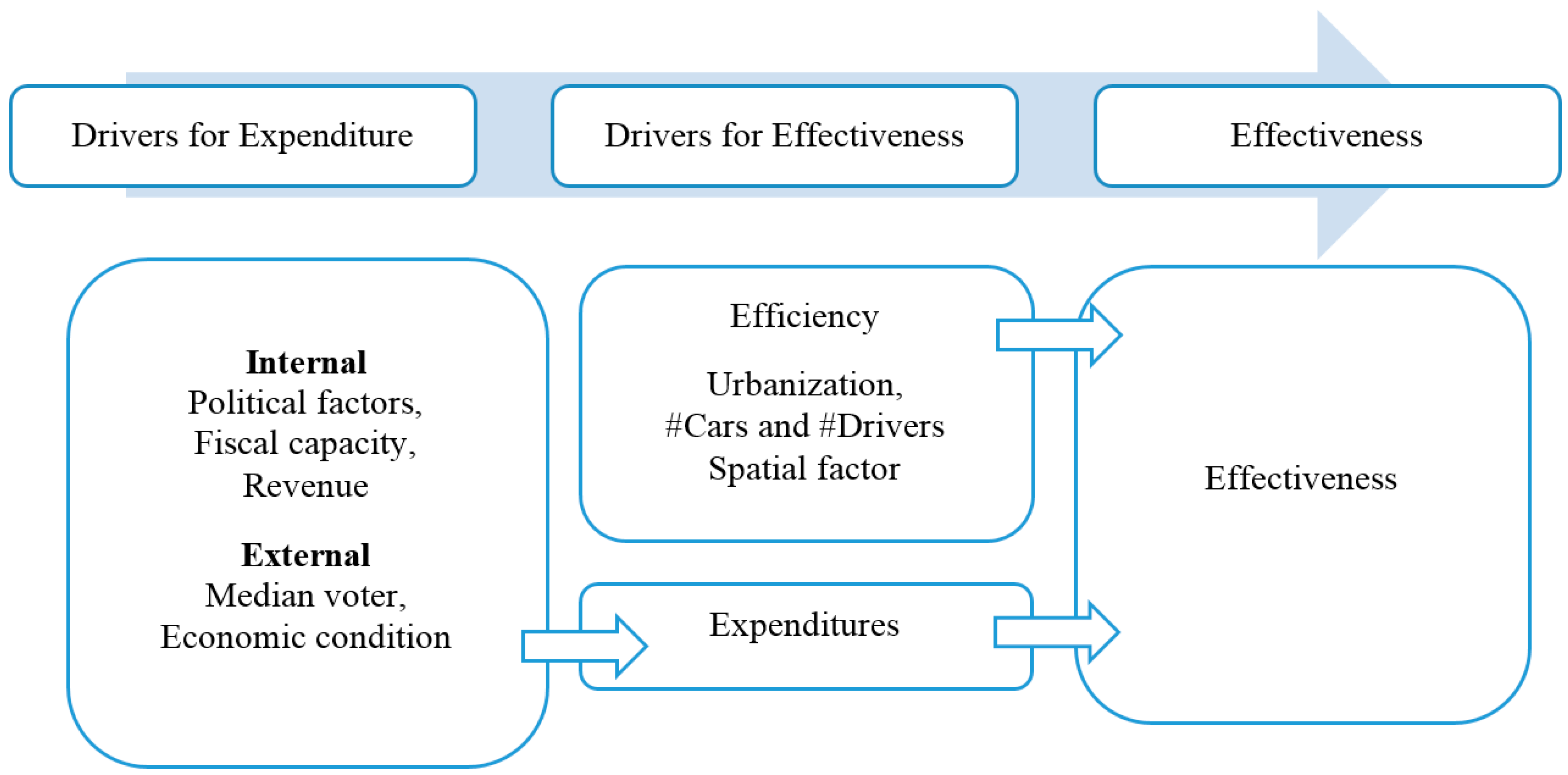
As seen in Figure 4, to investigate the relationship between efficiency and effectiveness, we set the two-stage regression model. At the first stage, we examine the determinants of highway expenditure, in which the model considers political factors, fiscal capacity, median voter, and economic condition as explanatory variables, according to prior literature [5,41,42,43,44]. At the second stage, we explain the dependent variable, effectiveness, as the function of the predicted value of expenditure by the first regression, efficiency scores by DEA, urbanization, the number of cars, the number of drivers, and spatial factor (rho) conducted by a spatial regression model.
The study operationalizes raw data in order to articulate variables and adjust for regression analysis. The effectiveness indicator, which is estimated using a combination of road condition, mobility, and safety, was modified by adding the constant 1 to take the log in the regression model (this is because the indicator’s original value has negative values that become imaginary numbers when taking the log). For road conditions, a higher value means better conditions. Mobility and safety are coded as the reciprocal of the annual average daily traffic (AADT) and the number of people fatally injured, respectively. Higher values of the reciprocals of these two variables indicate greater effectiveness.
The study suggests that effectiveness is determined by expenditures and other conditions such as the level of urbanization, the number of automobiles and drivers, and spatial factors while controlling other variables that affect expenditures at the first stage. In addition, efficiency scores are added as the independent variables so as to test for any meaningful relationship between efficiency and effectiveness.
3.3.3. Estimation Routine
We utilize the two-stage regression model approach. At the first stage, we use the fixed effects panel data model to estimate the predicted values of highway expenditure.
where α means the individual fixed effect and u is an error term.
At the second stage, the study employs the Spatial Autoregressive Panel Model to control the geographical spatial effect among continental states. Assuming that present performance depends on past performance, regression models include the lagged dependent variable on the right-hand side. We set the effectiveness indicator, which is produced by the principal component analysis, as the dependent variable. In addition, the other decomposed components (road condition, mobility, and safety) are also tested as dependent variables for comparison.
where W is the spatial matrix, α means the individual fixed effect, γ indicates the time effect, and u is an error term.
4. Results: Explaining the Relationship between Efficiency and Effectiveness
The study conducts a two-stage regression analysis. At the first stage, the highway expenditure is predicted with six explanatory variables using the fixed effects model. Table 8 reports that highway expenditure is associated with the following two factors: revenue and the median voter. The result shows one additional dollar of revenue for highway per capita increase highway expenditure per capita when holding the other variables constant. Median voter also increases highway expenditure which is consistent with prior literature [5,6].
Spatial regression results are reported in Table 9. Past performance is strongly and positively associated with each dependent variable. That is, one percentage change of past performance increases road condition by 0.5%, mobility by 0.95%, safety by 0.5%, and effectiveness indicator by 0.76%. Effects of the efficiency score, which is the key independent variable, are statistically significant. Since the efficiency score is calculated by data envelopment analysis that conducts a cross-sectional analysis, it cannot be used for comparing each state’s efficiency over time. Rather, it represents relative dominance compared with others in each year. The regression results reveal that efficiency has a positive effect on mobility, safety, and the effectiveness indicator. Thus, it can be said that a relatively dominant state in efficiency is likely also more effective in highway management. However, the efficiency variable has a negative effect on road condition. A possible explanation of the different effect directions could be found in the concept and measurement of efficiency and road condition. Efficiency can be represented by the ratio of output to input. Road condition would depend upon frequent maintenance such as resurfacing, which requires a higher level of input.
In terms of control variables, urbanized states with higher population densities are doing well on highway management, one percentage change of population density makes a 0.3% increase of the effectiveness indicator. The number of automobiles negatively affects effectiveness: road condition and safety. Rho represents the impact of spatial relations and shows positive effects, which means that a state is influenced by the surrounding states’ highway condition and management.
There is an interesting point regarding expenditure. Total highway expenditure predicted at the first stage has negative effects, whereas maintenance and capital outlay (investment) have positive effects on effectiveness. Particularly, maintenance expenditure is reported as having an all positive effect, though the effect on road conditions is not statistically significant. The results imply that specific direct spending on highways directly affects effectiveness, while indirect spending, such as operating expenses, does not enhance effectiveness.
5. Conclusions
This study begins with a question on why scholars rarely deal with the relationship between efficiency and effectiveness despite vast volumes of literature on both. Especially in the management of sustainable infrastructure, these two values are fundamental aims of governments that must respond to citizens’ needs under a limited budget. Despite this, previous literature regarding highway management has not empirically investigated the relationship between the two values. Therefore, this study focused on presenting empirical evidence for explaining how two core values of highway management are related and how efficiency and other determinants affect effectiveness. It is noteworthy that efficiency and effectiveness might not be compatible because efficiency is about cost reduction and effectiveness is about enhancing quality. As a result of quantitative models, however, this study found that the two significant values can be compatible with each other, highlighting developed definitions and measurements for them.
The findings show significant effects of efficiency on effectiveness of highway management. A more efficient government does the “right things” in terms of highway management, particularly better mobility and safety as well as overall effectiveness. Thus, it can be said that a government which does “things right” is likely to be more effective than an inefficient government. In addition, regarding expenditure on highways, maintenance and investment (capital outlay) enhance effectiveness as shown by the evidence that maintenance expenditure positively affects mobility, safety, and overall effectiveness, and investment has a significant impact on the mobility and the overall effectiveness indicator. This implies that direct spending on highways is important to improve the effectiveness of highway management. Furthermore, the study suggests ways to measure efficiency and effectiveness and states the kinds of inputs, outputs, and outcomes that are appropriate for this measurement. This also provides a useful example for students and practitioners.
As highlighted, the contributions of this study to theory and practice are: (1) the relationship between efficiency and effectiveness are empirically investigated, proposing developed measurements and methods such as multiple input and output factors; (2) the proposed concept of efficiency and effectiveness of highway management can be applied to the field of sustainability management; and (3) the empirical models using efficiency and effectiveness suggests new strategies of managing performance of sustainability in which state and local governments have been working together beyond the sector and level of public and private organizations.
Despite the contributions of this study, there are several limitations. First, entire state-level data relies on annual construction and, thus, needs more accurate data sets such as from the local level. We hope that scholars in the field of sustainability can build upon the relationship between efficiency and effectiveness by identifying key factors at the local, regional, and national level. Future research should focus on structures and procedures of highway management that can explain resolutions to overcome the barriers to performance management by using a simulation model. Also, the next step should include ways of computing the index of efficiency-effectiveness combined by using objective measures derived from secondary datasets such as detailed socioeconomic factors. More importantly, an in-depth interview with working professionals who fully understand highway management in sustainability is expected to provide validity of future research.
Acknowledgments
This research was supported by a grant (MPSS-NH-2015-82) through the Disaster and Safety Management Institute funded by Ministry of Public Safety and Security of Korean Government and also partially supported by the Ministry of Education of the Republic of Korea and the National Research Foundation of Korea (NRF-2016S1A3A2924563).
Author Contributions
NakHyeok Choi designed this research and analyzed data sets; Kyujin Jung contributed to elaborating theoretical and policy implications as well as structuring of this research.
Conflicts of Interest
The authors declare no conflict of interest.
References
- Mullins, D.R.; Pagano, M.A. Local budgeting and finance: 25 years of developments. Public Budg. Financ. 2005, 25, 3–45. [Google Scholar] [CrossRef]
- Kamensky, J.M. Budgeting for the state and local infrastructure: Developing a strategy. Public Budg. Financ. 1984, 4, 3–17. [Google Scholar] [CrossRef]
- Millar, A. Selecting capital investment projects for local governments. Public Budg. Financ. 1988, 8, 63–77. [Google Scholar] [CrossRef]
- Nunn, S. Budgeting for public capital. J. Urban Aff. 1990, 12, 327–344. [Google Scholar] [CrossRef]
- Congleton, R.; Bennett, R. On the political economy of state highway expenditures: Some evidence of the relative performance of alternative public choice models. Public Choice 1995, 84, 1–24. [Google Scholar] [CrossRef]
- Walden, M.L.; Eryuruk, G. Determinants of local highway spending in north carolina. Growth Chang. 2012, 43, 462–481. [Google Scholar] [CrossRef]
- Neshkova, M.I.; Guo, H. Public participation and organizational performance: Evidence from state agencies. J. Public Adm. Res. Theory 2012, 22, 267–288. [Google Scholar] [CrossRef]
- Rodriguez, A. Reformed County Government Structure and Service Delivery Performance: An Integrated Study of Florida Counties. Ph.D. Thesis, Florida International University, Miami, FL, USA, 1999. [Google Scholar]
- Mihaiu, D.M.; Opreana, A.; Cristescu, M.P. Efficiency, effectiveness and performance of the public sector. Rom. J. Econ. Forecast. 2010, 4, 132–147. [Google Scholar]
- Mandl, U.; Dierx, A.; Ilzkovitz, F. The Effectiveness and Efficiency of Public Spending; Directorate General Economic and Financial Affairs (DG ECFIN); European Commission: Brussels, Belgium, 2008. [Google Scholar]
- Karlaftis, M.G. A dea approach for evaluating the efficiency and effectiveness of urban transit systems. Eur. J. Oper. Res. 2004, 152, 354–364. [Google Scholar] [CrossRef]
- Starik, M.; Kanashiro, P. Toward a theory of sustainability management. Organ. Environ. 2013, 26, 7–30. [Google Scholar] [CrossRef]
- Bartle, J.R.; Devan, J. Sustainable highways. Public Works Manag. Policy 2006, 10, 225–234. [Google Scholar] [CrossRef]
- Sustainable Highways Initiative. Available online: https://www.sustainablehighways.dot.gov/overview.aspx#quest1 (accessed on 11 July 2017).
- Cormier, A.; Gilbert, R. Defining Sustainable Transportation. Available online: http://cst.uwinnipeg.ca/documents/Defining_Sustainable_2005.pdf (accessed on 3 July 2017).
- International Transport Forum. Transport Infrastructure Investment Options for Efficiency: Options for Efficiency; OECD Publishing: Paris, France, 2008. [Google Scholar]
- Le Grand, J. The theory of government failure. Br. J. Political Sci. 1991, 21, 423–442. [Google Scholar] [CrossRef]
- Worthington, A.C.; Dollery, B.E. Measuring efficiency in local governments’ planning and regulatory function. Public Prod. Manag. Rev. 2000, 23, 469–485. [Google Scholar] [CrossRef]
- Banker, R.D.; Janakiraman, S.; Natarajan, R. Analysis of trends in technical and allocative efficiency: An application to texas public school districts. Eur. J. Oper. Res. 2004, 154, 477–491. [Google Scholar] [CrossRef]
- Barrow, M.; Wagstaff, A. Efficiency measurement in the public sector: An appraisal. Fisc. Stud. 1989, 10, 72–97. [Google Scholar] [CrossRef]
- Brueckner, J.K. A test for allocative efficiency in the local public sector. J. Public Econ. 1982, 19, 311–331. [Google Scholar] [CrossRef]
- Taylor, L.L. Allocative inefficiency and local government. J. Urban Econ. 1995, 37, 201–211. [Google Scholar] [CrossRef]
- Herman, R.D.; Renz, D.O. Board practices of especially effective and less effective local nonprofit organizations. Am. Rev. Public Adm. 2000, 30, 146–160. [Google Scholar] [CrossRef]
- Forbes, D.P. Measuring the unmeasurable: Empirical studies of nonprofit organization effectiveness from 1977 to 1997. Nonprofit Volunt. Sect. Q. 1998, 27, 183–202. [Google Scholar] [CrossRef]
- Liket, K.C.; Maas, K. Nonprofit organizational effectiveness: Analysis of best practices. Nonprofit Volunt. Sect. Q. 2015, 44, 268–296. [Google Scholar] [CrossRef]
- Thordarson, T.B. Use of Funds in a Nonprofit Organization as Predictor of Organizational Effectiveness and Efficiency. Ph.D. Thesis, Andrews University, Berrien Springs, MI, USA, 2014. [Google Scholar]
- Herman, R.D.; Renz, D.O. Theses on nonprofit organizational effectiveness. Nonprofit Volunt. Sect. Q. 1999, 28, 107–126. [Google Scholar] [CrossRef]
- Eisinger, P. Organizational capacity and organizational effectiveness among street-level food assistance programs. Nonprofit Volunt. Sect. Q. 2002, 31, 115–130. [Google Scholar] [CrossRef]
- Cameron, K. A study of organizational effectiveness and its predictors. Manag. Sci. 1986, 32, 87–112. [Google Scholar] [CrossRef]
- Cameron, K.S.; Whetten, D.A. Organizational Effectiveness: A Comparison of Multiple Models; Academic Press: New York, NY, USA, 1983. [Google Scholar]
- Kushner, R.J.; Poole, P.P. Exploring structure-effectiveness relationships in nonprofit arts organizations. Nonprofit Manag. Leadersh. 1996, 7, 119–136. [Google Scholar] [CrossRef]
- Jimenez, B.S.; Pagano, M.A. What factors affect management quality? State infrastructure management and the government performance project. Public Works Manag. Policy 2011, 17, 124–151. [Google Scholar] [CrossRef]
- Salerno, C.S. On the Technical and Allocative Efficiency of Research-Intensive Higher Education Institutions. Ph.D. Thesis, The Pennsylvania State University, Old Main, PA, USA, 2002. [Google Scholar]
- Sherman, H.D.; Zhu, J. Service Productivity Management: Improving Service Performance Using Data Envelopment Analysis (DEA); Springer: New York, NY, USA, 2006. [Google Scholar]
- AASHTO. Available online: http://www.transportation.org/home/organization/ (accessed on 30 June 2017).
- FHWA. Available online: http://ops.fhwa.dot.gov/perf_measurement/index.htm (accessed on 30 June 2017).
- Qiu, L. Performance Measurement for Highway Winter Maintenance Operations. Ph.D. Thesis, The University of Iowa, Iowa City, IA, USA, 2008. [Google Scholar]
- Chan, C.Y.; Huang, B.; Yan, X.; Richards, S. Investigating effects of asphalt pavement conditions on traffic accidents in tennessee based on the pavement management system (pms). J. Adv. Transp. 2010, 44, 150–161. [Google Scholar] [CrossRef]
- Islam, S.; Buttlar, W.; Aldunate, R.; Vavrik, W. Measurement of pavement roughness using android-based smartphone application. Transp. Res. Rec. J. Transp. Res. Board 2014, 2457, 30–38. [Google Scholar] [CrossRef]
- Settich, J.F. Need and Politics: A Study of Federal Highway Funding and State Road Status Data between 1983 and 2000. Ph.D. Thesis, University of Illinois at Chicago, Chicago, IL, USA, 2003. [Google Scholar]
- Wang, W.; Hou, Y.; Duncome, W. Determinants of pay-as-you-go financing of capital projects: Evidence from the states. Public Budg. Financ. 2007, 27, 18–42. [Google Scholar] [CrossRef]
- Alt, J.E.; Lowry, R.C. Divided government, fiscal institutions, and budget deficits: Evidence from the states. Am. Political Sci. Rev. 1994, 88, 811–828. [Google Scholar] [CrossRef]
- Hou, Y.; Smith, D. Do state balanced budget requirements matter? Testing two explanatory frameworks. Public Choice 2010, 145, 57–79. [Google Scholar] [CrossRef]
- McGranahan, L. State budgets and the business cycle: Implications for the federal balanced budgets amendment debate. Econ. Perspect. 1999, 23, 3–17. [Google Scholar]
Figure 1.
Graph for efficiency concept.
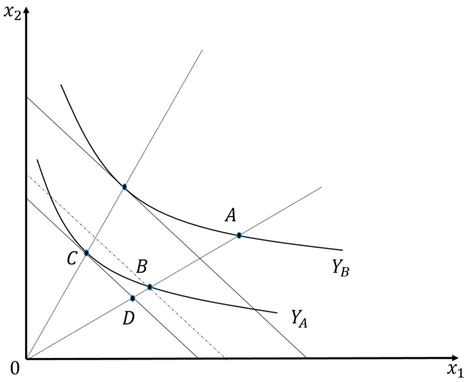
Figure 2.
Framework of Efficiency and Effectiveness [10].
Figure 2.
Framework of Efficiency and Effectiveness [10].
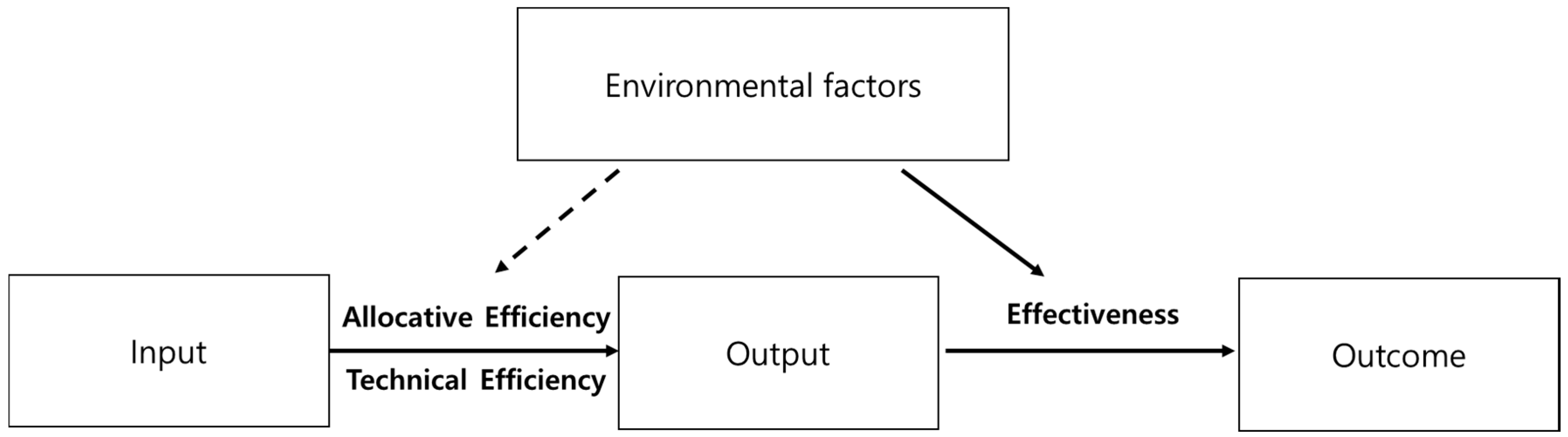
Figure 3.
Graph for data envelopment analysis (DEA) adapted from [20] (p. 83).
Figure 3.
Graph for data envelopment analysis (DEA) adapted from [20] (p. 83).

Figure 4.
Research Framework.


Table 1.
Matrix of Effectiveness and Efficiency.
| Ineffective | Effective | |
|---|---|---|
| Efficient | 3rd best practice | Best practice |
| Inefficient | Worst practice | 2nd best practice |
Table 2.
Input and Output factors for DEA.
| Input and Output Factors | Description | Data Source | |
|---|---|---|---|
| Input | Highway investment | State capital outlay and maintenance expenditure (SF-12) | Highway Statistics (2000–2008, 2012–2013) |
| Highway maintenance | |||
| Output | Length of lanes | Estimated lane-miles (HM-81) | |
| DVMT | Daily vehicle-miles traveled (HM-81) | ||
Table 3.
DEA Result Examples: Rankings and Technical Efficiency Scores (TES).
| 2000 | 2005 | 2012 | |||||||
|---|---|---|---|---|---|---|---|---|---|
| Ranking | State | TES | Ranking | State | TES | Ranking | State | TES | |
| Top 10 states | 1 | GA | 1 | 1 | CA | 1 | 1 | GA | 1 |
| 1 | ID | 1 | 1 | NH | 1 | 1 | NH | 1 | |
| 1 | OH | 1 | 1 | SC | 1 | 1 | NM | 1 | |
| 1 | SD | 1 | 1 | SD | 1 | 1 | SC | 1 | |
| 5 | SC | 1 | 5 | WV | 1 | 1 | VA | 1 | |
| 6 | CA | 0.98 | 6 | GA | 1 | 6 | WV | 1 | |
| 7 | NH | 0.94 | 7 | NM | 1 | 7 | CA | 0.9 | |
| 8 | LA | 0.85 | 8 | ND | 0.98 | 8 | NC | 0.79 | |
| 9 | MD | 0.85 | 9 | VA | 0.93 | 9 | MO | 0.77 | |
| 10 | WI | 0.85 | 10 | WI | 0.86 | 10 | DE | 0.76 | |
| Bottom 10 states | 39 | WY | 0.54 | 39 | MI | 0.52 | 39 | ND | 0.39 |
| 40 | UT | 0.54 | 40 | TX | 0.51 | 40 | KS | 0.38 | |
| 41 | NM | 0.54 | 41 | RI | 0.50 | 41 | RI | 0.38 | |
| 42 | NV | 0.53 | 42 | KS | 0.47 | 42 | NV | 0.36 | |
| 43 | KS | 0.53 | 43 | IL | 0.46 | 43 | NY | 0.36 | |
| 44 | ND | 0.52 | 44 | OR | 0.45 | 44 | UT | 0.35 | |
| 45 | CO | 0.50 | 45 | WA | 0.43 | 45 | IL | 0.34 | |
| 46 | PA | 0.44 | 46 | NY | 0.42 | 46 | NJ | 0.28 | |
| 47 | NY | 0.41 | 47 | FL | 0.40 | 47 | VT | 0.26 | |
| 48 | NJ | 0.41 | 48 | NJ | 0.31 | 48 | WA | 0.17 | |
Table 4.
Variable Description and Data Source for Principal Component Analysis (PCA).
| Variable | Description | Source |
|---|---|---|
| Road condition | Highway Statistics | |
| Mobility | Reciprocal of Annual Average Daily Traffic (AADT)/lane-miles | |
| Safety | Reciprocal of the number of people fatally injured/lane-miles |
Table 5.
Effectiveness Indicators for States’ Highway Management.
| 2000 | 2005 | 2012 | |||||||
|---|---|---|---|---|---|---|---|---|---|
| Rank | State | Score | Rank | State | Score | Rank | State | Score | |
| Effectiveness indicator | 1 | ND | 3.39 | 1 | ND | 2.64 | 1 | WV | 1.53 |
| 2 | WV | 1.14 | 2 | WV | 1.27 | 2 | VA | 0.90 | |
| 3 | VA | 0.62 | 3 | VA | 0.61 | 3 | SD | 0.81 | |
| 4 | WY | 0.58 | 4 | MT | 0.56 | 4 | MT | 0.73 | |
| 5 | SD | 0.44 | 5 | SD | 0.45 | 5 | WY | 0.72 | |
| 44 | MI | −0.44 | 44 | MD | −0.42 | 44 | MD | −0.34 | |
| 45 | CT | −0.46 | 45 | RI | −0.43 | 45 | FL | −0.36 | |
| 46 | MA | −0.56 | 46 | MA | −0.53 | 46 | MA | −0.44 | |
| 47 | CA | −0.60 | 47 | CA | −0.58 | 47 | CA | −0.52 | |
| 48 | NJ | −0.64 | 48 | NJ | −0.63 | 48 | NJ | −0.55 | |
| Road condition | 1 | GA | 97.18 | 1 | NV | 92.65 | 1 | GA | 89.95 |
| 2 | WY | 81.06 | 2 | GA | 92.31 | 2 | NV | 87.34 | |
| 3 | FL | 80.95 | 3 | FL | 82.70 | 3 | FL | 83.22 | |
| 4 | KS | 74.32 | 4 | KS | 81.14 | 4 | TN | 79.70 | |
| 5 | AL | 74.24 | 5 | MT | 77.97 | 5 | AL | 77.82 | |
| 44 | CA | 17.31 | 44 | CA | 31.46 | 44 | CA | 34.85 | |
| 45 | OR | 12.21 | 45 | CT | 24.31 | 45 | MA | 33.32 | |
| 46 | MA | 11.05 | 46 | MA | 23.95 | 46 | NJ | 32.38 | |
| 47 | MO | 10.47 | 47 | RI | 16.16 | 47 | CT | 31.64 | |
| 48 | NJ | 9.61 | 48 | NJ | 12.01 | 48 | RI | 18.57 | |
| Safety | 1 | ND | 195.52 | 1 | WV | 187.05 | 1 | WV | 210.08 |
| 2 | WV | 169.81 | 2 | ND | 136.85 | 2 | VA | 162.45 | |
| 3 | VA | 136 | 3 | VA | 132.17 | 3 | SD | 135.43 | |
| 4 | NC | 106.72 | 4 | NC | 109.94 | 4 | NC | 132.00 | |
| 5 | ME | 105.01 | 5 | ME | 107.31 | 5 | WY | 129.86 | |
| 44 | MI | 19.79 | 44 | MA | 19.81 | 44 | MA | 27.43 | |
| 45 | AZ | 16.80 | 45 | AZ | 15.72 | 45 | AZ | 23.50 | |
| 46 | FL | 13.27 | 46 | FL | 11.71 | 46 | FL | 17.82 | |
| 47 | CA | 13.18 | 47 | CA | 11.68 | 47 | CA | 17.66 | |
| 48 | NJ | 11.44 | 48 | NJ | 11.34 | 48 | NJ | 14.42 | |
| Mobility | 1 | ND | 0.74 | 1 | ND | 0.65 | 1 | WV | 0.16 |
| 2 | WV | 0.15 | 2 | WV | 0.14 | 2 | MT | 0.11 | |
| 3 | SD | 0.11 | 3 | SD | 0.11 | 3 | SD | 0.11 | |
| 4 | WY | 0.10 | 4 | MT | 0.11 | 4 | WY | 0.09 | |
| 5 | MT | 0.10 | 5 | WY | 0.09 | 5 | ND | 0.09 | |
| 44 | CT | 0.01 | 44 | MD | 0.01 | 44 | FL | 0.02 | |
| 45 | FL | 0.01 | 45 | FL | 0.01 | 45 | MD | 0.01 | |
| 46 | MA | 0.01 | 46 | MA | 0.01 | 46 | MA | 0.01 | |
| 47 | CA | 0.01 | 47 | CA | 0.01 | 47 | NJ | 0.01 | |
| 48 | NJ | 0.01 | 48 | NJ | 0.01 | 48 | CA | 0.01 | |
Table 6.
Variable Description and Data Source. NCSL = National Conference of State Legislatures; NASBO = National Association of State Budget Officers.
Table 6.
Variable Description and Data Source. NCSL = National Conference of State Legislatures; NASBO = National Association of State Budget Officers.
| Variable | Description | Data Source |
|---|---|---|
| Effectiveness indicator | Combination of road condition, mobility, and safety | Author’s computation with PCA |
| Road condition | ||
| Mobility | Reciprocal of Annual Average Daily Traffic (AADT)/lane-miles | |
| Safety | Reciprocal of the number of people fatally injured/lane-miles | |
| Efficiency score | Theta from DEA (Data Envelopment Analysis) | Author’s computation with DEA |
| Urbanization | Population density | U.S. Census |
| Automobiles per capita | Number of automobiles/population | Highway Statistics |
| Drivers/driving age people | Number of drivers/population of driving age | Highway Statistics |
| Maintenance expenditure per capita | Maintenance expenditure per capita | Highway Statistics |
| Capital outlay per capita | Capital outlay per capita | Highway Statistics |
| Highway expenditure per capita | Highway expenditure per capita | U.S. Census |
| Revenue for highway per capita | Revenue for highway per capita | Highway Statistics |
| Own source ratio | 1 − (Intergovernmental revenue/Total revenue) | U.S. Census |
| Republican governor | Republican governor = 1, otherwise = 0 | NCSL, NASBO |
| Divided government | 1 = governor’s party equal to the majority partisanship of legislature, 0 = otherwise | NCSL, NASBO |
| Median voter | Median income of household | U.S. Census |
| Economic condition | Unemployment rate | U.S. Census |
Table 7.
Descriptive Statistics.
| Variable | N | Mean | Std. Dev. | Min | Max |
|---|---|---|---|---|---|
| Effectiveness indicator | 528 | 0.996 | 4.015 | 0.000004 | 39.818 |
| Road condition | 528 | 2.443 | 0.242 | 1.775 | 2.971 |
| Mobility | 528 | 0.54 | 0.087 | 0.009 | 0.741 |
| Safety | 528 | 58.355 | 38.409 | 10.992 | 213.692 |
| Efficiency score | 528 | 0.687 | 0.194 | 0.161 | 1 |
| Urbanization | 528 | 192.870 | 257.903 | 5.307 | 1201.497 |
| Automobiles per capita | 528 | 0.441 | 0.079 | 0.151 | 0.641 |
| Drivers/driving age people | 528 | 894.833 | 62.973 | 704.746 | 1115.696 |
| Maintenance expenditure per capita | 528 | 0.047 | 0.033 | 0.002 | 0.271 |
| Capital outlay per capita | 528 | 0.239 | 0.112 | 0.072 | 1.115 |
| Highway expenditure per capita | 528 | 0.376 | 0.151 | 0.159 | 1.579 |
| Revenue for highway per capita | 528 | 0.409 | 0.194 | 0.156 | 1.952 |
| Own source ratio | 528 | 73.339 | 5.882 | 47.161 | 85.491 |
| Republican governor | 528 | 0.534 | 0.499 | 0 | 1 |
| Divided government | 528 | 0.526 | 0.499 | 0 | 1 |
| Median income of household | 528 | 46306.91 | 7965.03 | 29359 | 72483 |
| Unemployment rate | 528 | 5.198 | 1.512 | 2.3 | 11.1 |
Table 8.
First Stage Regression with the Fixed Effects Model.
| Highway Expenditure Per Capita | ||
|---|---|---|
| Coef. | S.E. | |
| Revenue for highway per capita | 0.238 *** | 0.030 |
| Own source ratio | 0.001 | 0.001 |
| Republican governor | 0.011 | 0.007 |
| Divided government | 0.009 | 0.007 |
| Median voter | 0.01 *** | 0.001 |
| Economic condition | −0.002 | 0.003 |
| Constant | −0.030 | 0.064 |
| Number of observations | 432.000 | |
| Number of groups | 48.000 | |
| Prob > F | 0.001 | |
Note: *** p < 0.01. Time-period: 11 waves (2000–2013 except 2009–2011). Forty-eight continental U.S. states.
Table 9.
Second Stage Regression Using the Spatial Autoregressive Panel Model.
| Road Condition | Mobility | Safety | Effectiveness Indicator | |
|---|---|---|---|---|
| Coef. (S.E.) | Coef. (S.E.) | Coef. (S.E.) | Coef. (S.E.) | |
| Past performance (lagged dependent variable) | 0.542 *** | 0.952 *** | 0.520 *** | 0.769 *** |
| (0.031) | (0.042) | (0.041) | (0.041) | |
| Efficiency score | −0.084 * | 0.167 *** | 0.081 *** | 0.079 *** |
| (0.046) | (0.032) | (0.030) | (0.023) | |
| Urbanization | −0.005 | 0.319 ** | 0.749 *** | 0.311 *** |
| (0.198) | (0.131) | (0.135) | (0.097) | |
| Automobiles per capita | −0.111 * | −0.007 | −0.088 ** | −0.031 |
| (0.058) | (0.040) | (0.039) | (0.030) | |
| Drivers/driving age people | −0.020 | 0.084 | 0.237 * | 0.106 |
| (0.202) | (0.138) | (0.130) | (0.099) | |
| Highway expenditure per capita | 0.045 | −0.164 *** | −0.080 | −0.109 *** |
| (0.079) | (0.053) | (0.050) | (0.038) | |
| Maintenance expenditure per capita | 0.004 | 0.043 *** | 0.022 ** | 0.025 *** |
| (0.017) | (0.012) | (0.011) | (0.008) | |
| Capital outlay per capita | −0.011 | 0.107 *** | 0.041 | 0.054 ** |
| (0.043) | (0.029) | (0.028) | (0.021) | |
| Rho (spatial) | 0.059 | 0.224 *** | 0.387 *** | 0.408 *** |
| (0.058) | (0.058) | (0.046) | (0.056) | |
| Variance | 0.017 *** | 0.008 *** | 0.007 *** | 0.004 *** |
| (0.001) | (0.001) | (0.001) | (0.001) | |
| Number of observations | 480 | 480 | 480 | 480 |
| Number of groups | 48 | 48 | 48 | 48 |
| Log-likelihood | 318.0782 | 494.6012 | 518.8232 | −636.5719 |
Note: *** p < 0.01, ** p < 0.05, * p < 0.1. Time-period: 11 waves (2000–2013 except 2009–2011). Forty-eight continental U.S. states. All variables are log-transformed.
© 2017 by the authors. Licensee MDPI, Basel, Switzerland. This article is an open access article distributed under the terms and conditions of the Creative Commons Attribution (CC BY) license (http://creativecommons.org/licenses/by/4.0/).
Share and Cite
MDPI and ACS Style
Choi, N.; Jung, K. Measuring Efficiency and Effectiveness of Highway Management in Sustainability. Sustainability 2017, 9, 1347. https://doi.org/10.3390/su9081347
AMA Style
Choi N, Jung K. Measuring Efficiency and Effectiveness of Highway Management in Sustainability. Sustainability. 2017; 9(8):1347. https://doi.org/10.3390/su9081347
Chicago/Turabian StyleChoi, NakHyeok, and Kyujin Jung. 2017. "Measuring Efficiency and Effectiveness of Highway Management in Sustainability" Sustainability 9, no. 8: 1347. https://doi.org/10.3390/su9081347
Note that from the first issue of 2016, this journal uses article numbers instead of page numbers. See further details here.