Experimental Investigations and Numerical Simulation of Thermal Performance of a Horizontal Slinky-Coil Ground Heat Exchanger

1
Key Laboratory of Energy Thermal Conversion and Control of Ministry of Education, School of Energy and Environment, Southeast University, Nanjing 210096, Jiangsu, China
2
School of Hydraulic, Energy and Power Engineering, Yangzhou University, Yangzhou 225127, Jiangsu, China
*
Authors to whom correspondence should be addressed.
Sustainability 2017, 9(8), 1362; https://doi.org/10.3390/su9081362
Submission received: 6 July 2017
/
Revised: 27 July 2017
/
Accepted: 31 July 2017
/
Published: 3 August 2017
(This article belongs to the Section Energy Sustainability)
Abstract
:A model test system of horizontal slinky coil ground heat exchanger (HSCGHE) was established according to the similarity theory. A 2-D mathematical model of HSCGHE was built and experimentally validated. Experimental and numerical investigations of effects of different parameters on the thermal behavior of HSCGHE were undertaken. The results show that the heat release rate of the slinky coil and soil temperature around it increase as the inlet fluid temperature of coil increases. The soil temperature operated in intermittent mode can get a recovery, and thus the heat release rate of the coil can be improved effectively. For a given condition, reducing the coil central interval distance can increase the heat release rate of the HSCGHE, but also results in the decrease of the heat release rate per unit length of the coil. Therefore, the coil central interval distance cannot be decreased without limit. At the same time, the thermal performance of HSCGHE is related to the ground surface wind velocity. The heat release rate in the sandstone is the largest, followed by sand, the lowest for clay. Additionally, with the increase of buried depth of coil, the heat release rate increases, but the increase degree gradually becomes small. Thus, the buried depth cannot be too deep and should be determined by thermal performance, excavation cost and safety requirements.
1. Introduction
Ground-coupled heat pump (GCHP) is one of the most efficient means to provide space heating and cooling of buildings [1]. It utilizes the ground as heat source/sink of the heat pump and provides higher energy efficiencies than conventional air-conditioning system due to the more favorable temperature level in the ground [2], thus it has become more and more popular for heating and cooling application in various kinds of buildings [3,4].
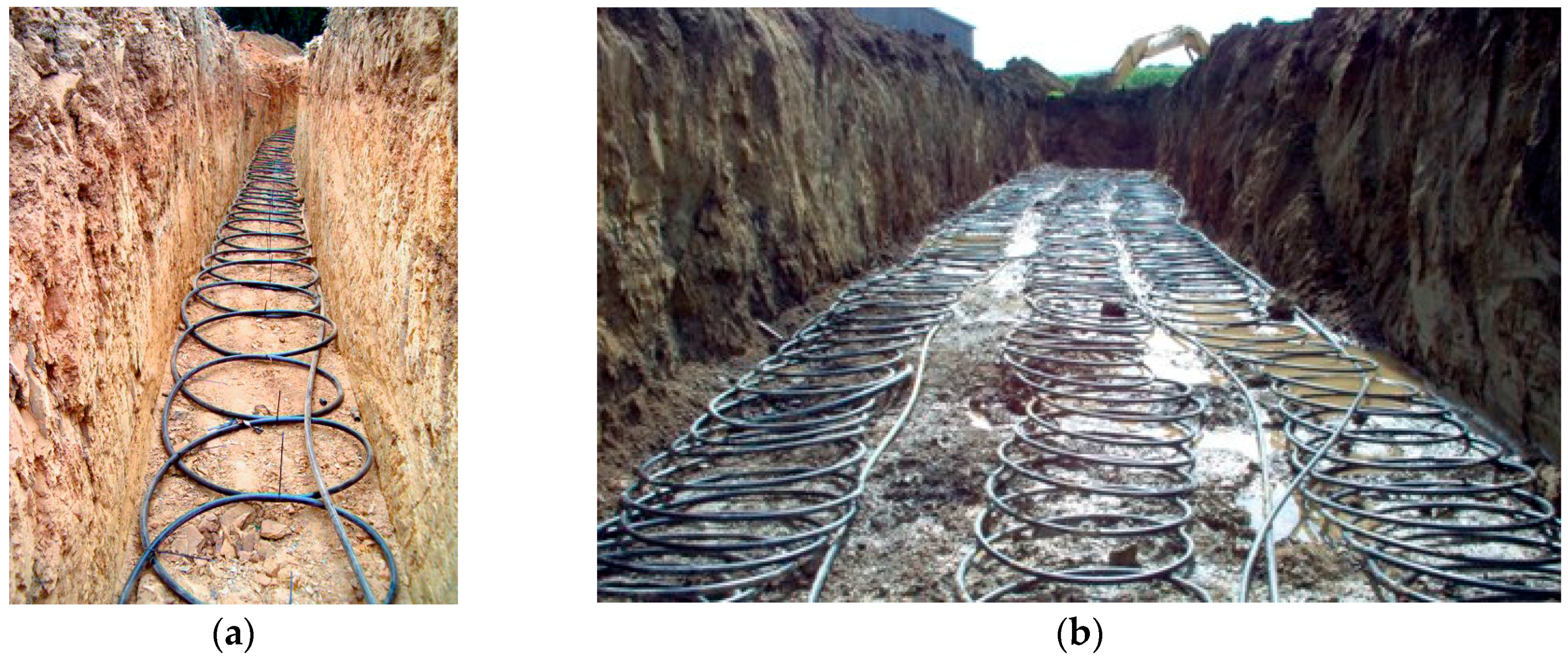
A GCHP system is usually composed of a heat pump and a ground heat exchanger (GHE). The GHE can be horizontally installed in trenches or vertically in boreholes [5]. Vertical GHEs need smaller buried pipe area and can obtain the most efficient system performance. However, the depth of borehole in which vertical GHEs are installed often varies from 40 to 100 m, thus resulting high drilling costs. Horizontal GHEs, consisting of straight or coil pipes that are installed in a trench with a depth of 1.5–2.0 m, can provide a viable alternative solution that obtains a good compromise between high efficiency and low costs. However, conventional straight horizontal GHE requires a large amount of land surface, this limits its application [6]. As an alternative, horizontal slinky coil ground heat exchangers (HSCGHE) (Figure 1) have higher pipe density and need less land area and excavation work than conventional straight horizontal GHE. Because of these advantages, the HSCGHE has been widely concerned for the case that needs high efficiency and low costs [6].
Some studies discuss the thermal performance of horizontal GHEs, by either numerical modeling or experimental investigation. Pulat et al. [7] assessed the system performance of a ground coupled heat pump with horizontal ground heat exchangers by using different system parameters for winter climate condition of Bursa, Turkey. A set of experimental device previously used for cooling cycle was changed to experimentally investigate the effects of various factors on operation performance of system and heat pump unit. The results showed that the coefficient of performance (COP) of the system and heat pump unit range 2.46–2.58 and 4.03–4.18, respectively. Cui et al. [8] proposed a transient heat source model of ring coil to study the thermal conduction surrounding the buried spiral coils, and the explicit solutions for the temperature response were obtained using the Green’s function theory and image method. Xiong et al. [9] presented the development and validation of a slinky coil GHE model intended for use in building simulation programs. The model uses analytical ring source solutions to compute temperature response functions for both horizontal and vertical slinky coil GHEs. Go et al. [10] presented an optimization design algorithm for a GCHP system with horizontal spiral coil GHE. A 3-D numerical analysis model was proposed to simulate the thermal characteristics of a horizontal spiral coil GHE, and the model was verified by thermal response tests. Li et al. [11] developed a numerical model to investigate the operation characteristics of a GCHP system with horizontal spiral-coil. The model considers the geothermal gradient and the varying ambient air temperature. Wang et al. [12] developed a ring-coil model by using Green’s function method. The spiral coil is regarded as a series of ring coils that inject or extract heat in/from a semi-infinite medium. Yoon et al. [13] investigated experimentally the heat transfer rate of the horizontal slinky coil, spiral-coil and U-type GHEs installed in a steel box. The heat exchange rate of these three kinds of horizontal GHEs was evaluated by in situ thermal response tests. The results indicated that the U-type GHE has the highest heat exchange rate per pipe length. Kupiec et al. [14] proposed a one-dimensional numerical model for a horizontal GHE. The model was validated by comparison with the experimental results presented in literature. Kim et al. [15] investigated experimentally the thermal performance of horizontal slinky coil and spiral coil GHEs installed in a 5 m × 1 m × 1 m steel box. Various parameters that affect the performance of horizontal GHE were examined by numerical simulation and validated with the experimental results. The results indicated that the horizontal coil GHEs is better than the slinky GHE. Dasare et al. [16] presented a numerical model for predicting the thermal performance of horizontal GHEs with a different type. A numerical simulation was undertaken to study the effects of the major factors that determine the thermal characteristics of the GHEs. The results indicated that the soil thermal conductivity and flow rate are two important factors affecting the heat transfer performance of GHEs, and the effect of installation depth on the thermal performance of GHEs can be neglected. Congedo et al. [17] compared the thermal performance of three types of horizontal GHEs, linear, helical and slinky; the most important parameters for the evaluation of their performance were obtained by changing different parameters that affect the thermal performance of the GHEs. It can be found that the depth of the horizontal GHE has little effect on the system performance. Go et al. [18] presented a new performance evaluation method for horizontal GCHP system with rainfall infiltration. The effect of rainfall infiltration on the thermal performance of shallow trenches was performed by infiltration analyses, and a numerical simulation was also performed to analyze the effect of rainfall infiltration on the performance of the horizontal GHE. Sofyan et al. [19] developed a new 3-D transient mathematical model of a horizontal GHE. The influence of seasonal variations of ground temperature on the performance of the horizontal GHE was considered in the model by an energy balance in the ground surface, and the seasonal variations of ground temperature are expressed as an internal source term. Chong et al. [20] proposed a 3-D mathematical model of HSGHE. Based on the model, the numerical investigation of the effects of different loop pitches, loop diameters, ground thermal properties and operation modes were performed. The results indicated that system parameters have a significant effect on the thermal performance of the system. Wu et al. [21] monitored the performance of a GCHP with HSCGHE and the tested results were used to predict the thermal performance of HSCGHE with different slinky diameters and slinky interval distances. It can be concluded that the average COP of the horizontal-coupled GCHP was 2.5 and there was no significant difference in the heat extraction of the slinky heat exchanger at different coil diameters. Fujii et al. [22,23] compared the heat exchange rates of double-layer slinky-coil horizontal GHEs and single-layer horizontal GHEs by long term cooling and heating tests. The results showed that the heat exchange rate per unit land area is obviously improved by using double-layer horizontal GHEs. The optimum depth of the upper layer GHE was 1.5 m when the lower layer was located at 2.0 m. Li et al. [24] proposed a moving ring source model to investigate the thermal performance of a spiral GHE under groundwater flow. The experiments were also carried out to test the soil temperature variations of two different spiral GHE layouts with different groundwater velocities. The results showed that the groundwater flow has a large effect on the system performance, and thus it is important to measure the water direction and velocity before system construction. Selamat et al. [25] examined the methods to optimize horizontal GHEs design through using different layouts and pipe materials. The optimum objective was obtained by a CFD simulation. The comparable heat exchange rates for all cases are obtained for an equal trench length. Naili et al. [26] have conducted the energy and exergy calculating of horizontal GHE under hot climatic condition of northern Tunisia. The overall heat transfer coefficient and heat exchange rate of GHE were calculated, and the effects of GHE length, diameter and the fluid flow rate on the thermal performance of GHE were investigated. It can be seen that the energy efficiency are found to vary between 18% and 52%, and the exergy efficiency lies between 12% and 36%. Gao et al. [27] proposed a horizontal GHE with a rain garden. The experiments were undertaken in a sandy soil container and the results indicated that water immigration was possible by the thermal action of the horizontal GHE. Verda et al. [28] investigated the operation conditions for a horizontal GSHP by an exergetic analysis. The main reasons of performance reduction were evaluated, and the optimal depth and position of the GHE were obtained to change the operating parameters.
However, the above studies are mainly focused on the numerical investigations of thermal characteristics of horizontal slinky coil GHE and its model construction. Few studies have been performed to deeply investigate the effects of various factors such as inlet temperature, coil central interval distance, ground surface wind velocity, soil type, buried depth and possible ground water flow on thermal performance of HSCGHE. Specifically, the influence mechanism of different factors on the thermal behavior of HSCGHE was still less understood. In this paper, a model test system of HSCGHE was built according to the similarity theory. A 2-D heat transfer model of HSCGHE was developed and validated by the experimental results. The effects of various parameters on the thermal performance of HSCGHE were experimentally and numerically investigated.
2. Experimental Investigation
2.1. Experimental Device
The experimental device, which is a model test system designed based on the similarity theory, was installed in Yangzhou University [29]. As shown in Figure 2, the experimental system includes a soil tank, constant temperature water tank, circulation water pump, flow meter, adjust valves, and data logger system. The water was heated by the electric heaters installed in the water tank and then the heat was discharged into the soil by the slinky-coil GHE. Different inlet water temperature can be set by adjusting the power of the heaters. The flow adjust valve and flow meter were utilized to set and test the flow rate of circulating water, respectively. The temperature data were tested and recorded at a time-interval by a data logger system.
The soil tank in this model test system was a wooden box sized 1.6 m × 1.2 m × 0.6 m and full of soil. The HSCGHE, which is made by PU pipe with 8 mm outer diameter and 5 mm internal diameter (shown in Figure 3), was constructed by horizontally wounding the PU pipe with 0.2 m diameter and 0.04 m center spacing. To explore the influence laws of ground surface wind velocity on the thermal behavior of the slinky coil, an adjustable fan was used to create different ground surface wind velocities, and a 25-mm-thick insulating plate was covered at the top of the soil tank to simulate zero wind velocity case. To guarantee the heat transfer similarity between the model test device and the corresponding physical prototype, similarity theory [30] was cited here to ensure the Reynolds number in the model test device is equal to that in the physical prototype, and the corresponding parameters in the two cases can also be obtained as listed in Table 1.
2.2. Temperature Measurement System
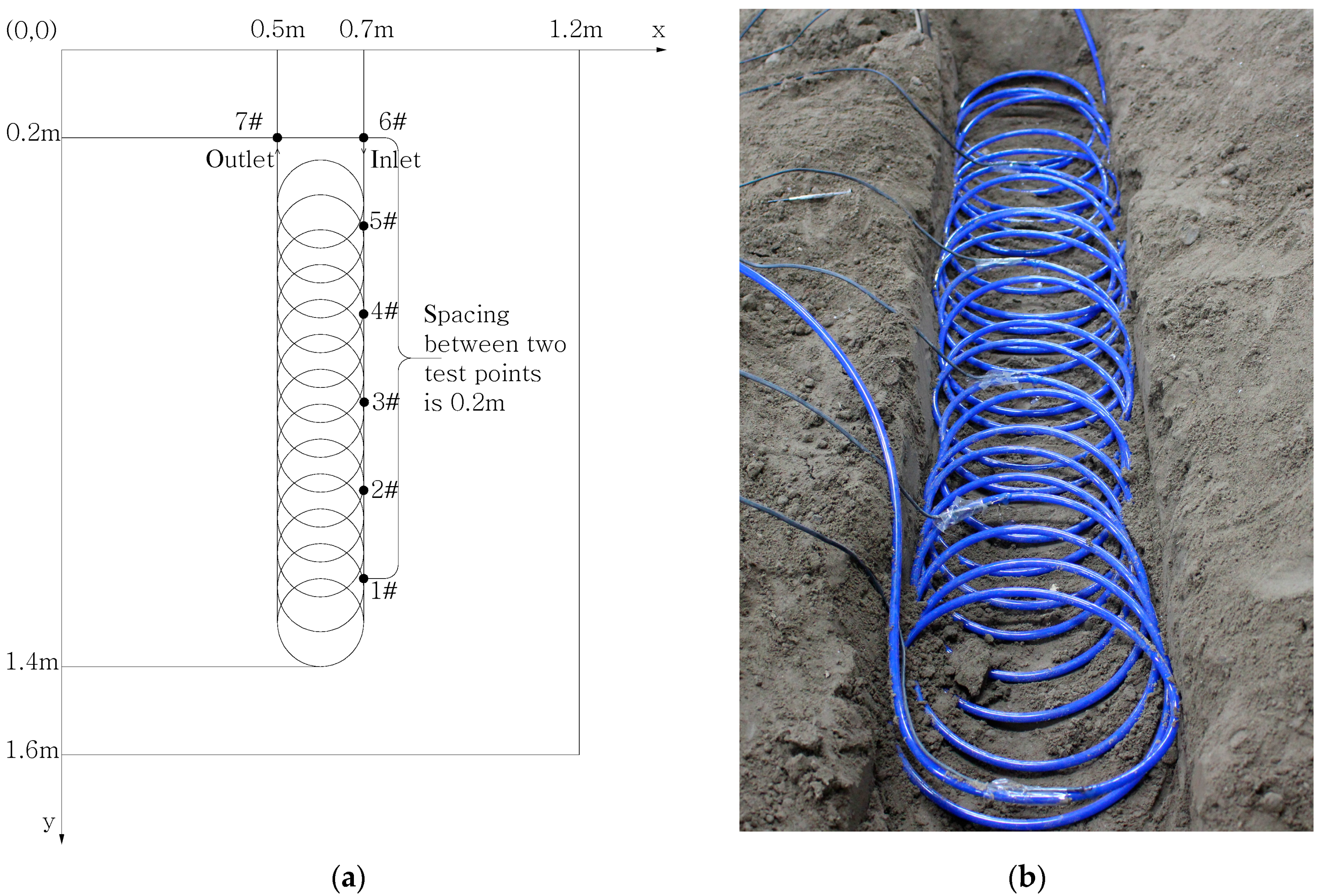
As shown in Figure 3, seven thermocouples (named from 1# to 7#) were wrapped on the outer wall of pipe along the coil to measure the fluid temperature variation along the coil. Among them, the inlet and outlet fluid temperature of coil were measured by 6# and 7# thermocouples, respectively. The soil temperature distribution around the coil pipe was monitored by 19 thermocouples (named from 8# to 26#) buried at different locations in the soil (shown in Figure 4). All temperature sensors were made with T-type thermocouples. The Agilent data logger instrument shown in Figure 2 was used to automatically record the values of all temperature test points.
2.3. Experimental Performance Analysis
2.3.1. Experimental Data Processing
During this experiment, the heat release rate of coil and soil excess temperature were calculated through using the experimental data.
The heat release rate of coil can be obtained from:
where Qg is the heat release rate of coil. cp is the specific heat of fluid. is the mass flow rate in the coil. Tin and Tout are the fluid temperature of coil at the inlet and outlet, respectively.
The heat release rate per unit pipe length, ql, can be expressed as:
where Lp is the coil length in a trench.
To further investigate the soil temperature variation characteristics, the excess temperature of the soil, defined as the difference between the tested temperature and original temperature of soil, is used here to reflect the soil temperature rise velocity. It is a positive value for heat release and negative value for heat extraction and can be written as:
where θ is the soil excess temperature. Tg and T0 are the tested soil temperature and corresponding original temperature, respectively.
2.3.2. Error Analysis
In this experiment, measurement and calculation error estimations are included in the error analysis. The temperature and flow rate are the measured parameters, and the calculated parameters include the heat release rate and soil excess temperature.
The errors δxi and relative errors δRxi for the measured parameters are expressed as:
where A is the upper limit of the measurement range, and γi is the accuracy grade.
To estimate the relative error of the calculated parameters, the basic root-sum-square method [31] was used here. If F is a function of independent measured variables xi, the relative error δRF of the F can be expressed as:
The relative errors for all parameters can be calculated through Equations (4)–(6), and the typical values for the major parameters in the experiments are listed in Table 2.
2.4. Experimental Results and Discussions
2.4.1. Effects of Inlet Water Temperature
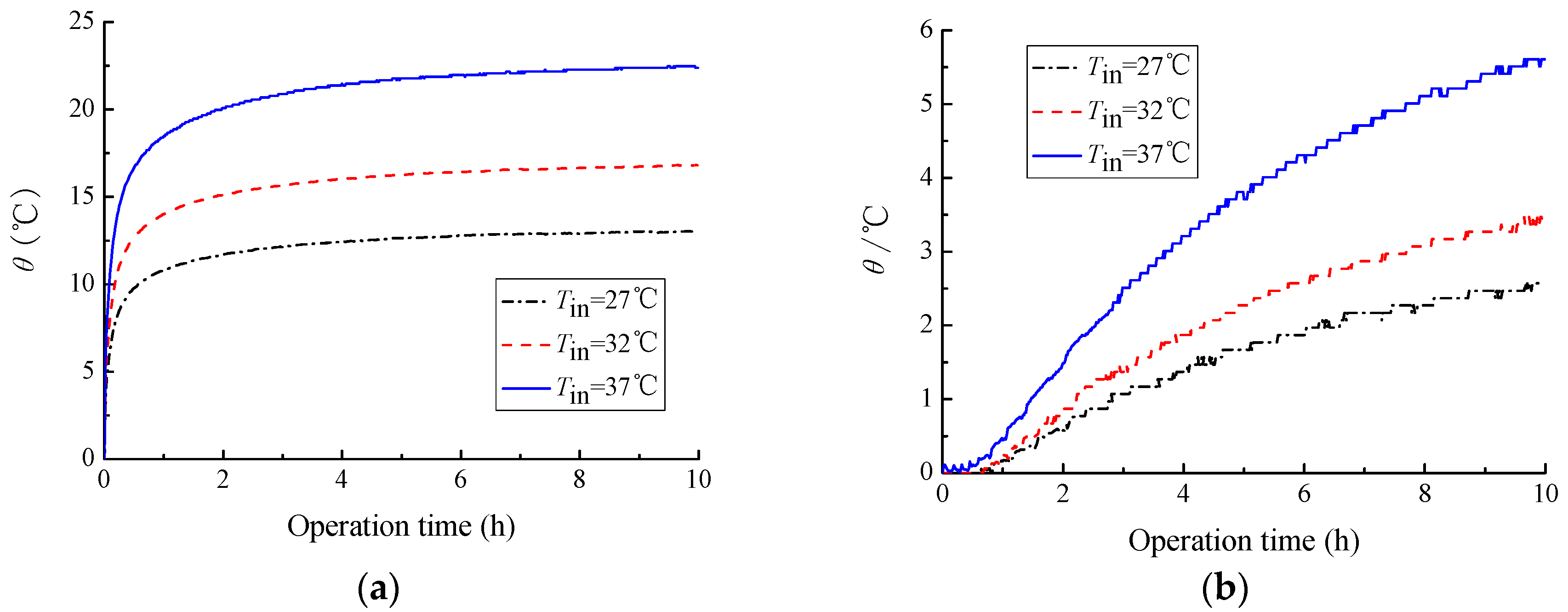
In this paper, water temperatures of 37, 32, and 27 °C, which are usually used in engineering, were chosen to explore the influences of inlet temperatures on thermal characteristics of HSCGHE. The initial ground temperature before the experiment is 11.3 °C, and the experimental results are presented in Figure 5 and Figure 6.
It can be seen in Figure 5 that the heat release rate of the HSCGHE decreases with time and gradually reaches a stable value. The higher the inlet temperature, the larger the stable value of heat release rate. As shown in Figure 5, the corresponding stable value of heat release rate at the inlet temperatures of 37, 32 and 27 °C are, respectively, 300.7, 260.3 and 214.6 W. The increment of heat release rate are 45.7 W and 86.1 W for increasing from 27 to 32 °C and from 27 to 37 °C, respectively. The latter is almost twice the former. Therefore, increasing the inlet temperature can effectively enhance the thermal performance of the HSCGHE.
Figure 6 shows that increment in the temperature of inlet water of the coil can also results in the increase of the soil excess temperature. However, the increase of the degree decreases as the distance from the center line increases. For example, when the operation time is 6 h, for x = 0.6 m where the location is at the center line of coil, the soil excess temperature are, respectively, 12.8, 16.4 and 22.1 °C for the inlet temperatures of 27, 32 and 37 °C. However, for x = 0.8 m, the corresponding values are 1.87, 2.57 and 4.31 °C, respectively. Thus, the increase in inlet temperature can lead to the increase in soil excess temperature, and as the distance from the center line of the coil increases, the increase of the degree becomes progressively smaller.
2.4.2. Effect of the Intermittent Operating Mode
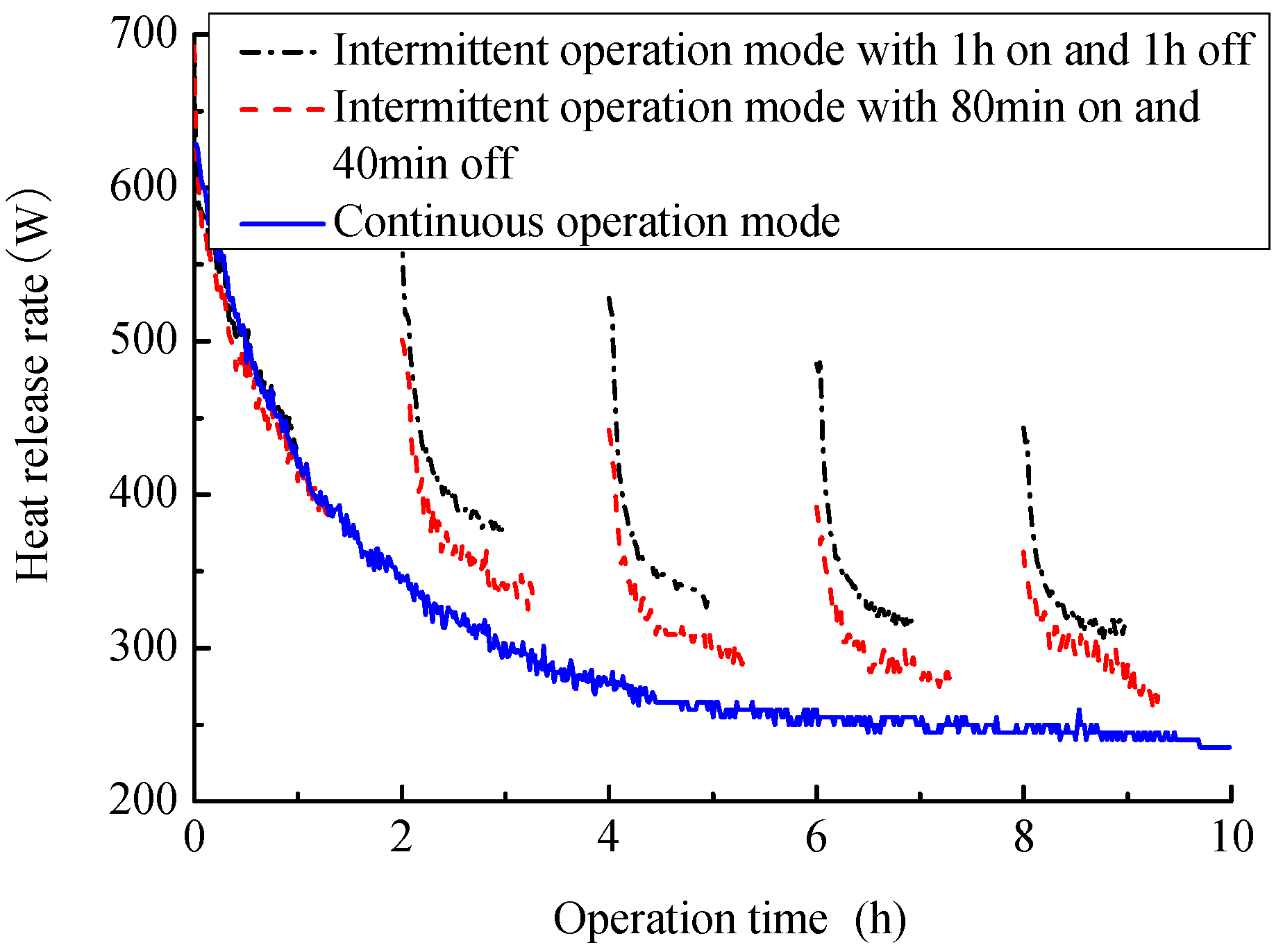
To explore the influences of intermittent operation modes, three operation modes were used in this experiment, which include continuous operating mode, intermittent operating mode with 80 min on and 40 min off, and intermittent operating mode with 1 h on and 1 h off. During the experiment, the inlet water temperature and test time are set to 37 °C and 10 h, respectively. The test results are presented in Figure 7 and Figure 8.
It can be seen in Figure 7 that the heat release rate of coil in the continuous operation mode decreases with the time and gradually reaches a stable value. For the intermittent modes, the heat release rate can obtain a rise for each interval. For instance, the average heat release rate at the end of 10 h operation is 300.7 W for the continuous operation mode, and the corresponding values are, respectively, 351.4 and 391.2 W for the intermittent mode with 80 min on and 40 min off and intermittent mode with 1 h on and 1 h off. This is mainly because the soil temperature operated in intermittent operation modes can recover during the intermittent time, and thus the heat transfer performance can be improved. As shown in Figure 8, the soil temperature rise rate operated in two intermittent operation modes are lower than that in the continuous operation mode, the restoration rate of soil temperature increases as the intermittent time increases, and thus the soil excess temperature decreases. For instance, when the operation time is 10 h, the soil excess temperature operated in the continuous operation mode is 22.4 °C, and the corresponding values are 13.6 and 9.9 °C for the intermittent mode with 1 h on and 1 h off and with 80 min on and 40 min off, respectively. It is obvious that compared with continuous operation mode, the soil excess temperature operated in the two intermittent modes decreases by 39.3% and 55.8%, respectively. Therefore, the soil temperature rise rate can be reduced by the intermittent operating control, and the heat release efficiency of coil and system operation performance can be improved.
2.4.3. Effect of the Coil Central Interval Distance
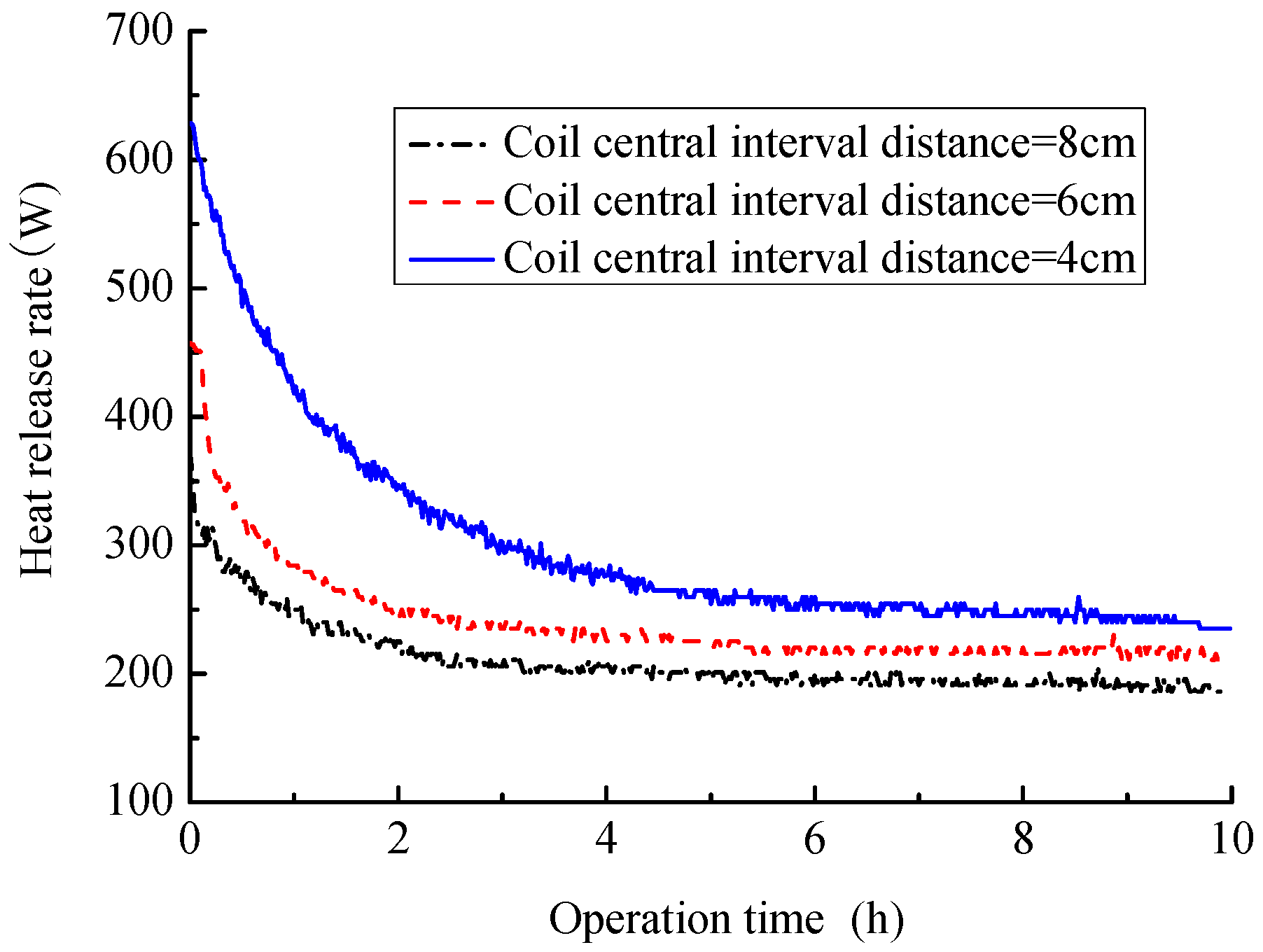
In a trench, the coil central interval distance determines the total coil length and corresponding heat exchange area. Thus, thermal performance of HSCGHE has relation with its central interval distance. To explore the influences of coil central interval distance on thermal characteristics of HSCGHE, three central interval distances including 4, 6, and 8 cm were used in the experiment, and the test results were presented in Figure 9, Figure 10 and Figure 11.
Figure 9 shows that a smaller coil central interval distance can contribute to a larger heat release rate. As shown in Figure 9, the heat release rate at the time of 10 h are, respectively, 186.2, 210.7 and 235.2 W for the coil central interval distance of 8, 6 and 4 cm. The main reason is that the coil length and corresponding heat exchange area increase as the coil central interval distance decreases, which help to enhance the heat transfer between the coil and soil around it. In Figure 10, we can further find that the heat release rate per unit length of coil will become small due to the decrease of coil central interval distance. For instance, when the coil central interval distance is 8 cm, the heat release rate per unit length of coil are 19.3 W/m, and the corresponding value is 15.3 W/m for 4 cm, 20.7% decrease compared with coil central interval distance of 8 cm. This means that the coil central interval distance cannot be too small and should be determined by considering the heat release rate, coil costs and available buried coil area.
Figure 11 shows the variation curves of soil excess temperature at x = 0.6 m and y = 0.2 m with time for different coil central interval distances. It can be observed that, when the coil central interval distance is constant, the soil excess temperatures increase with time and gradually reach to a stable value. With the increase of the coil central interval distance, the stable value decreases and corresponding time to be stable becomes shorter. For example, when the coil central interval distance is 8 cm, the steady value and steady time are about 16.5 °C and 8.5 h, respectively. However, for the coil central interval distance of 6 and 4 cm, the steady value and steady time are 19.8 °C and 6.6 h, and 21.8 °C and 5 h, respectively. The most possible reason is that reducing the coil central interval distance can increase the heat release rate and thus more heat is released into soil. This will inevitably increase the rise rate of soil temperature and heat diffusion time. Therefore, from the point of reducing thermal diffusion time and the cost of coils, the coil central interval distance should not be too small.
Based above analysis, we can conclude that a smaller coil central interval distance can contribute to a larger heat release rate, but also results in a smaller heat release rate per unit length of coil. Thus, the coil central interval distance cannot be too small and should be determined by the heat release rate, coil cost and available land area.
2.4.4. Effect of the Ground Surface Wind Velocity
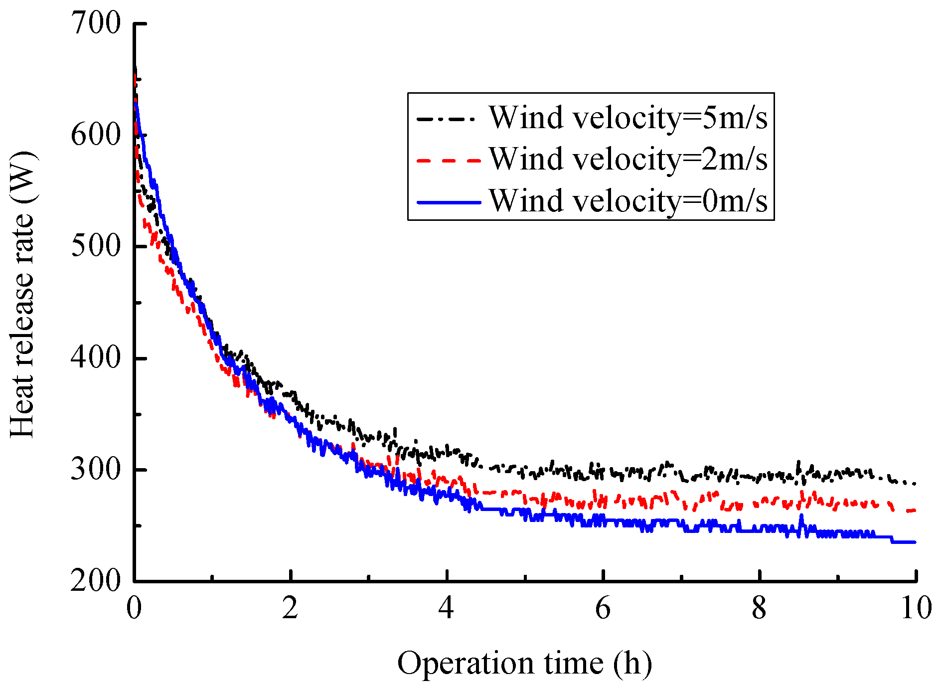
Due to the shallow buried depth of HSCGHE, its thermal performance can be easily influenced by the ground surface heat exchange conditions, especially ground surface wind velocity. To further study the effects of ground surface wind velocity, the experimental tests under the ground surface wind velocity of 0, 2, and 5 m/s were conducted and the experimental results were presented in Figure 12.
It can be seen in Figure 12 that the heat release rate increases as the surface wind velocity grows. As shown in Figure 12, the average heat release rate is 300.7 W for the wind velocity of 0 m/s, and the corresponding values are 311 and 334.2 W, respectively for the ground surface wind velocities of 2 and 5 m/s. Compared with 0 wind velocity, the heat release rate under wind velocities of 2 and 5 m/s increase, respectively, by 3.4% and 11.4%. The main reason is that a large surface velocity can enhance the convection heat transfer in the ground surface. Therefore, increasing wind velocity help to improve the heat release performance of HSCGHE.
3. Numerical Simulation
3.1. Physical Model
Heat transfer between the HSCGHE and the soil is a complicated process. To develop the heat transfer model, the following assumptions are made to simplify the problem.
- The initial temperature of the soil at the same depth is uniform and the soil is viewed as a type of isotropic, homogeneous rigid porous media.
- The HSCGHE is treated as a series of equally spaced straight pipes located in the same trench as slinky coil.
- The thermal properties of slinky coil, soil and fluid are constant.
- Groundwater flows only in the horizontal direction perpendicular to the trench.
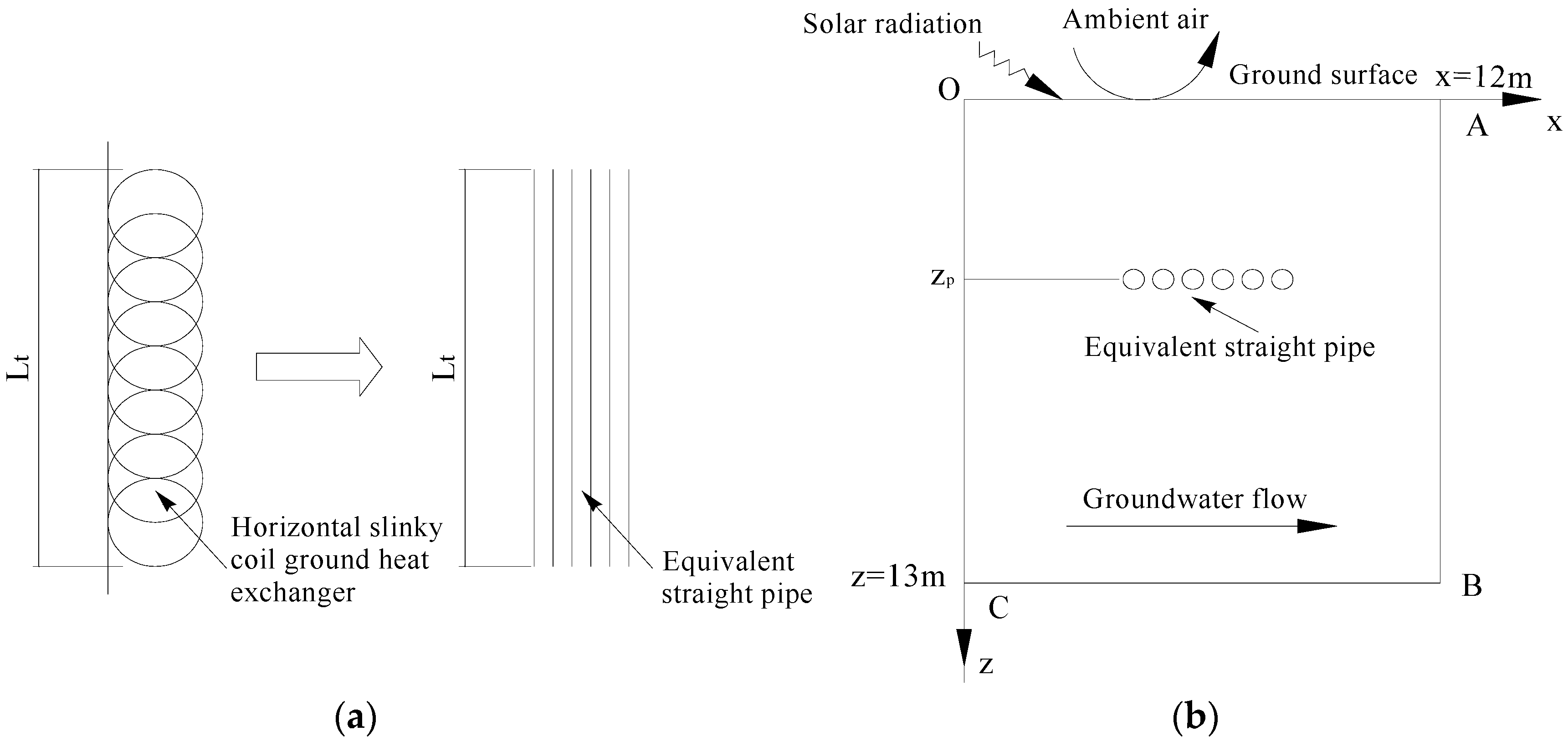
Based on the above assumptions, the heat transfer between the HSCGHE and soil around it can be viewed as the heat transfer between several equally spaced straight pipes and surrounding soil (shown in Figure 13), the number of the equally spaced straight pipes can be calculated by [32]
where n is the number of the equally spaced straight pipes. Lp is the total length of the slinky coil pipe. Lt is the length of the trench.
3.2. Mathematical Model
3.2.1. Heat Transfer Model of Soil outside Pipe
Soil is a typical porous media in which heat is transported based on three mechanisms: thermal conduction of the matrix and liquid of solid and thermal convection of moving liquid in the pore [33].
The heat transfer in the solid phase of the soil can be viewed as heat conduction, and the energy equation is
The heat transfer in the liquid phase of the soil include both thermal conduction and thermal convection of fluid, and thus the energy equation can be written as
The space proportion of liquid and solid in unit volume of the soil are designated as ε and (1 − ε), respectively, and Equations (8) and (9) can be expressed as
For a control volume, based on energy balance, Equations (10) and (11) can be unified as an equation and expressed as
where
where (ρcp)t is the total effective volumetric specific heat of the soil. (ρcp)s and (ρcp)f are the volumetric specific heat of solid phase and liquid phase of soil, respectively. λt is the total effective thermal conductivity of soil, while λs and λf are the thermal conductivity of solid phase and liquid phase of soil, respectively. qt is the total source/sink for the soil. qs and qf are the source/sink for solid and liquid phase.
3.2.2. Heat Transfer Model of Fluid along the Pipe Direction
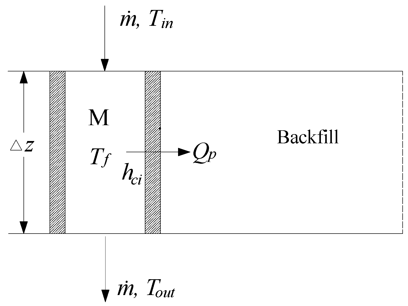
According to Assumption (3) that there is no contact thermal resistance between backfill material and pipe, the thermal resistance between the fluid inside pipe and backfills can be divided into two parts: convective heat transfer resistance inside the pipe and heat conduction resistance of the pipe wall. Thus, the total heat transfer resistance for an element pipe with a length of ΔZ can be expressed as [32]
where Rtotal, Rf, and Rp are the total thermal resistance from the fluid inside the pipe to the outer wall of pipe, convection thermal resistance and heat conduction thermal resistance of pipe wall, respectively. din and dout are, respectively, the inside and outside diameters of the equivalent straight pipe. λp is the thermal conductivity of the pipe. hci is the convective heat transfer coefficient of the fluid in the pipe, λf is the thermal conductivity of fluid inside pipe.
The temperature of fluid in the coil decreases as it moves along the coil length during summer operation. Heat from the warmer fluid is transferred into the soil surrounding the pipe through the pipe walls. Figure 14 shows the subdivision of the coil pipe into equally sized element pipe. According to the law of energy conservation, for an element pipe with a length of ΔZ (shown in Figure 14), the following energy balance equations can be obtained.
where M is the mass of the fluid in each element pipe. is the mass flow rate through the element pipe. cpf is the mass specific heat of the fluid in pipe. Tin and Tout are, respectively, the inlet and outlet fluid temperature of element pipe. Qp is the heat flux through the element pipe wall. Tg is the ground temperature.
3.3. Initial and Boundary Conditions
3.3.1. Initial Conditions
The initial conditions of soil and fluid inside pipe are viewed as the same:
The soil initial temperature can be calculated as follows [11]:
where TM is the annual mean ground temperature. A0 is the amplitude of annual temperature. ω is the angular frequency of annual temperature variations, ω = 0.000717 1/h; τ0 is the coldest day of a year; τ is the day evaluated, from 1 January; αs is the soil thermal diffusivity; and z is the depth of the ground.
3.3.2. Boundary Conditions
The boundary conditions of soil calculated region are taken as:
- (1)
- AB:
- (2)
- BC:
- (3)
- CO:
- (4)
- OA:where Qs is the surface heat flux into the ground. αs is the solar absorptivity. Qsun is the solar radiation intensity on the ground. ha is the convective heat transfer coefficient of the air. Ta is the temperature of the air.
3.4. Experimental Validation of the Model
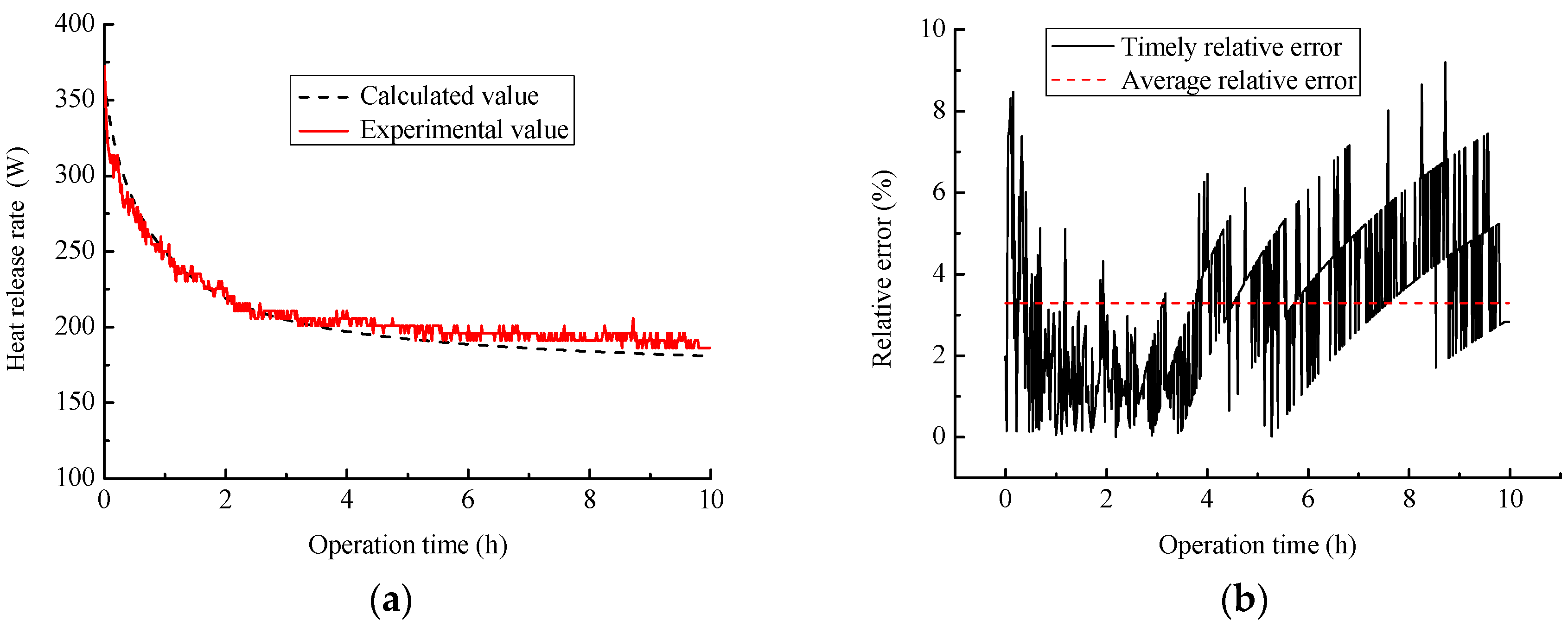
To validate the model developed above, experimental tests are performed on the test system shown in Figure 2, the values calculated by the model, and the corresponding experimental values of heat release rate of coil are compared. The results are shown in Figure 15.
It can be found in Figure 15a that the variation laws of heat release rate of coil are the same for the calculated and experimental values, and the calculating heat release rates are in agreement with the corresponding test results. Figure 15b shows that the maximum and average relative errors are 9.1% and 3.3%, respectively, which are allowed in practical engineering. This implies that the model established above can simulate effectively the thermal performance of the HSCGHE.
3.5. Calculated Results and Discussion
Considering the actual operation conditions, an intermittent operation mode with 10 h operation during daytime and 14 h off during night was utilized here. The equation is discretized by the finite volume method and TDMA algorithm is used to solve numerically the discrete equation group. The calculated conditions used in the numerical simulation are shown in Table 3 and the simulation results are presented in Figure 16, Figure 17, Figure 18, Figure 19, Figure 20 and Figure 21.
3.5.1. Effects of Groundwater Advection Velocity
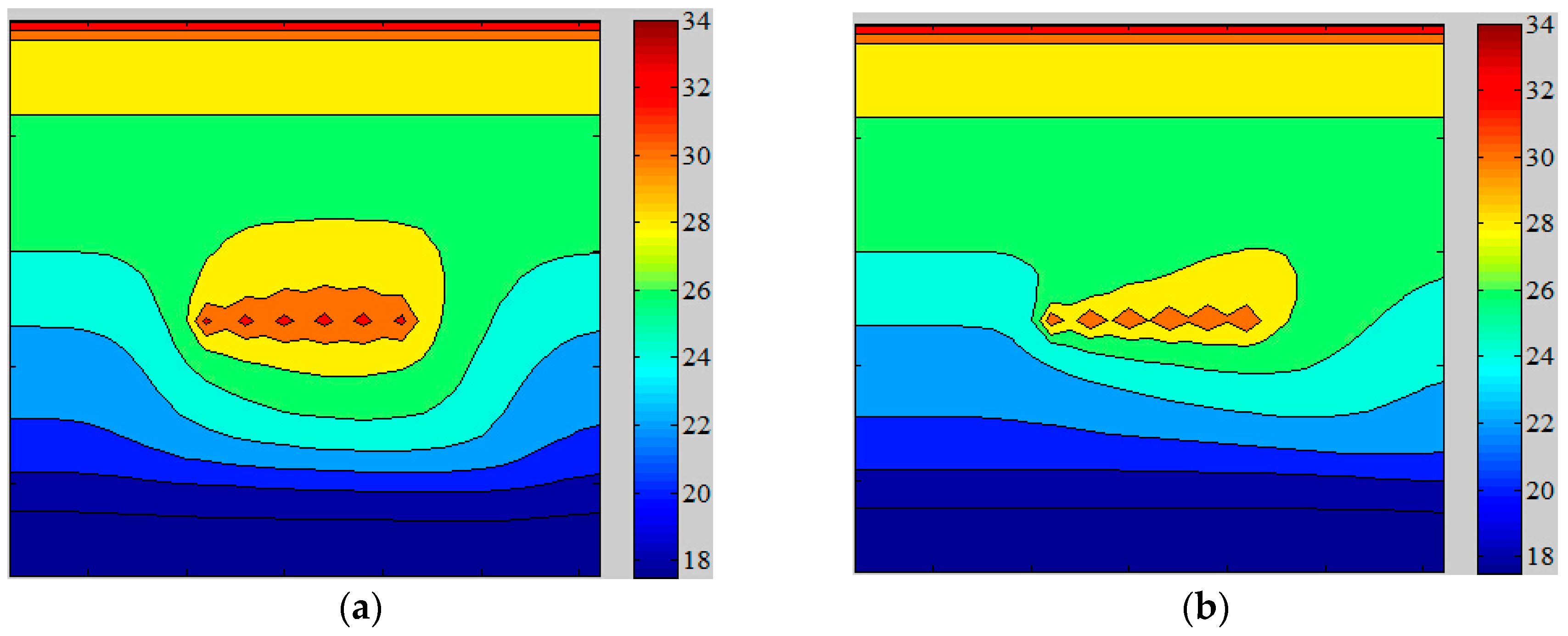
Numerical investigation on the thermal performance of HSCGHE with the advection velocity of 0, 50, 150 and 300 m/year were undertaken in the paper. The simulation results are presented in Figure 16 and Figure 17.
Figure 16 shows the temperature distribution of soil surrounding pipe for the advection velocity of 50 and 300 m/year. It can be found out that the soil temperature field has a migration along the groundwater flow direction. With the increase of groundwater advection velocity, the migration amplitude increases and the temperature of soil around the pipe decreases. This will improve the thermal performance of HSCGHE. As shown in Figure 17, the heat release rate of coil increases as the groundwater advection velocity increases. For example, the heat release rate of coil at the time of 90 days are 2.1, 2.3, 2.7, and 3.2 kW for the advection velocity of 0, 50, 150 and 300 m/year, respectively. The main reason is that the greater the groundwater advection velocity, the more heat is taken away by the groundwater, and the smaller the soil temperature rise degree. This implies that the existence of groundwater advection is conducive to the improvement of thermal performance of the HSCGHE. The greater is the groundwater advection velocity, the better is the thermal performance of coil.
3.5.2. Effects of Soil Type
To analyze the influences of soil type on the thermal performance of HSCGHE, clay, sand and sandstone were used here. Table 4 lists the values for their thermal properties, and the simulation results are presented in Figure 18 and Figure 19.
Figure 18 shows the variation curves of heat release rate of coil with time for these three soil types. It can be found that the heat release rate is the largest for sandstone, followed by sand, and the lowest is clay. As shown in Figure 18, when the operation time is 50 days, the heat release rates are 3.2, 3.6 and 4.6 kW for clay, sand and sandstone, respectively. Compared with clay, the heat release rate increases by 12.5% and 43.8%, respectively, for sand and sandstone. The main reason is that the soil with a large thermal conductivity has better heat conduction performance and thus the heat release rate can be improved more effectively. As shown in Table 3, sandstone has the highest thermal conductivity, followed by sand and the smallest is for clay, which results in that the slinky coil with sandstone has the maximum water temperature drop along length direction, followed by sand and clay. As shown in Figure 19, when the operation time is 40 days, the water temperature drops are 4.4, 5.2 and 6.9 °C for clay, sand and sandstone, respectively. This means that sandstone is the best and clay is the worst for improving the thermal performance of coil.
3.5.3. Effects of the Buried Depth
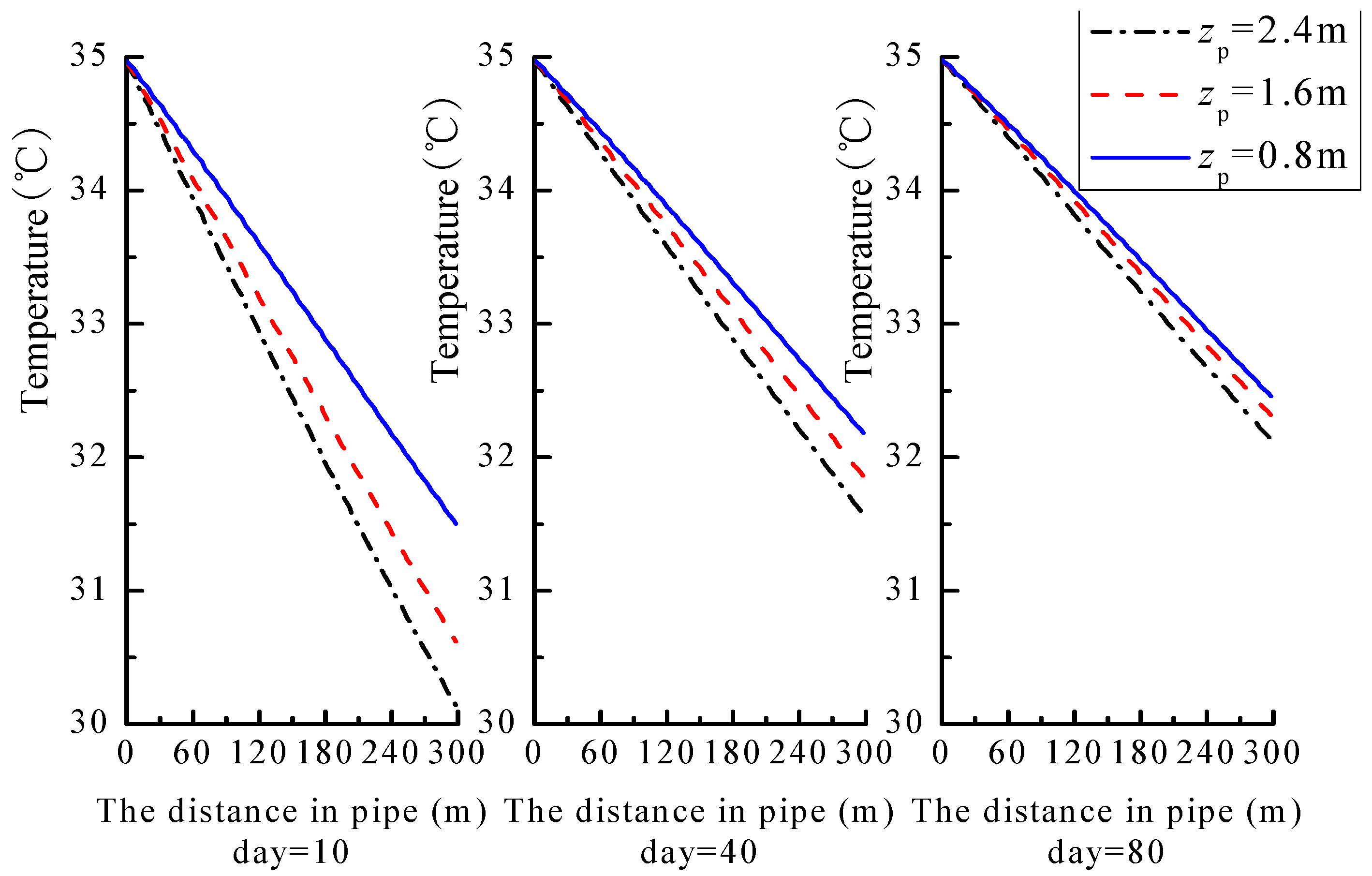
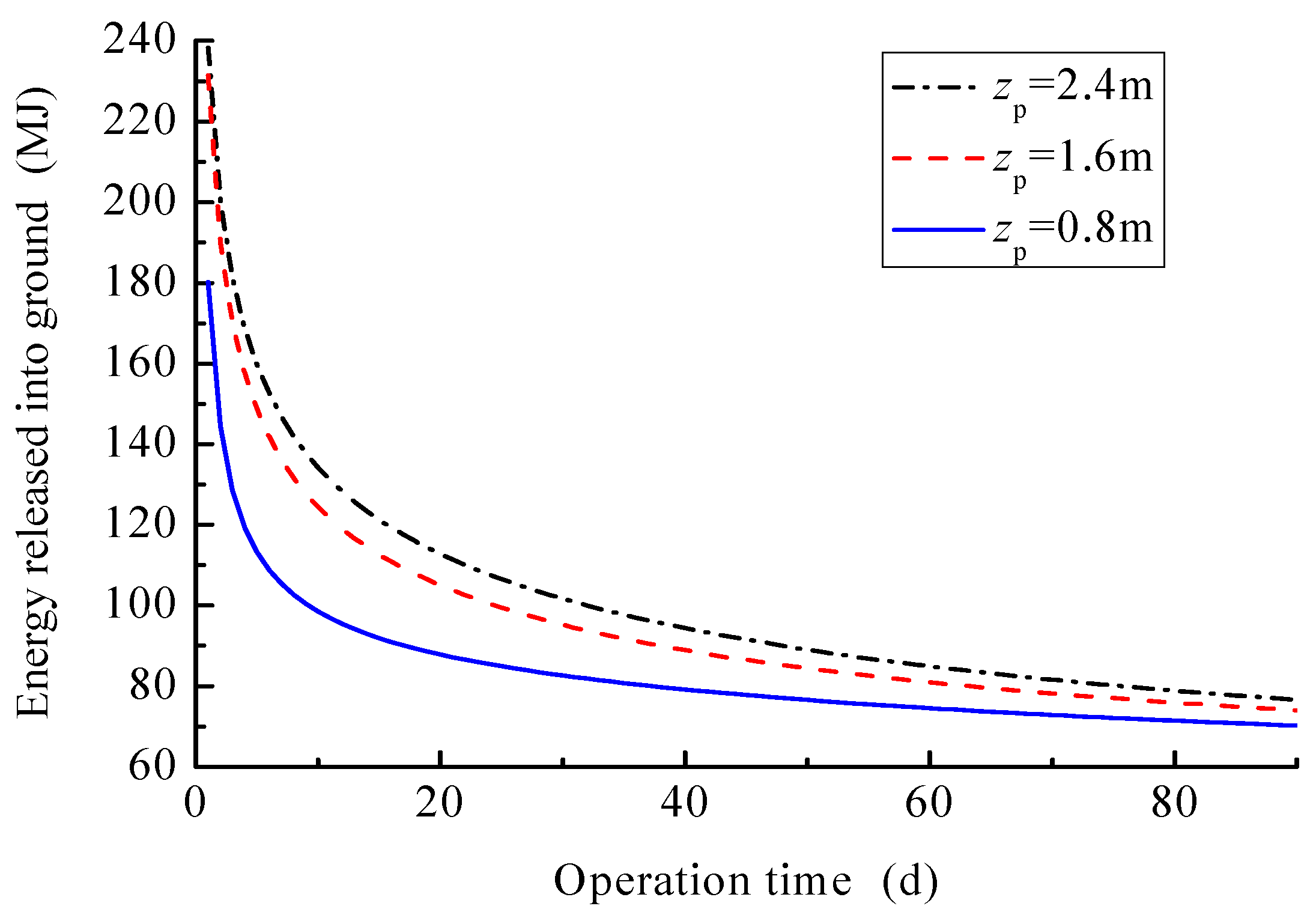
As mentioned above, the thermal performance of coil can be easily influenced by the surface heat exchange conditions due to its shallow buried depth. To further explore the influences of the buried depth on the thermal performance of coil, three depth conditions, 0.8, 1.6 and 2.4 m, are investigated and the calculated results are presented in Figure 20 and Figure 21. Figure 20 shows the variation curves of energy released into ground with operation time for different buried depths. Figure 21 presents the variation curves of water temperature along the pipe length for different buried depths.
In Figure 20, we can find that the energy released into ground by the coil increases as the buried depth increases. As shown in Figure 20, when the operation time is 40 days, the released energy are, respectively, 79.2, 85.3 and 87.9 MJ for the buried depth of 0.8, 1.6 and 2.4 m. Further analysis of Figure 20 can find that the increment and increasing rate of the released energy are, respectively, 6.1 MJ and 7.7% when the buried depth increases from 0.8 to 1.6 m, and the corresponding values are, respectively, 2.6 MJ and 3% when increases from 1.6 to 2.4 m. This means that, with the increase of buried depth, the influence of buried depth change on thermal performance is reduced. It can also be observed that, when increasing the buried depth, the released energy can be improved mostly during the first 20 days, but the increase rate becomes small after 20 days. As shown in Figure 21, during the early period of operation, the fluid temperature along pipe length declines largely, but it gradually becomes small with time. Thus, the thermal performance of slinky-coil can be effectively improved by increasing the buried depth mostly during the early operation time. However, the buried depth cannot be too deep and should be determined by the heat exchange performance, excavation cost and safety requirements of coil.
4. Conclusions
In this research, a model test system was established to study the thermal performance of HSCGHE. A two-dimensional heat transfer model of HSCGHE was developed and validated by the experimental results. The effects of different parameters on the thermal performance of HSCGHE were experimentally and numerically investigated. Based on above analysis, we can make the following conclusions.
- (1)
- The heat release rate of HSCGHE increases as the inlet temperature increases, and thus the thermal performance of HSCGHE can be enhanced effectively. Meanwhile, the increase of inlet temperature can also lead to an increase in soil excess temperature, and the increase degree becomes smaller as the distance from center line of coil increases.
- (2)
- The soil temperature operated in intermittent mode can recover: during each interval, the soil temperature restoration rate increases as the intermittent time increases, and thus the temperature rise rate of soil around the HSCGHE can be delayed. Therefore, under the condition of intermittent operation control strategy, the soil temperature rise rate can be reduced, and thus the heat release efficiency of the HSCGHE and system operation performance can be improved effectively.
- (3)
- A smaller coil central interval distance can contribute to a larger heat release rate, but also results in a smaller heat release rate per unit length of coil. Thus, the coil central interval distance cannot be too small and should be determined through considering the heat release rate, coil cost and available land area. At the same time, with the increase of the coil central interval distance, the sable value of soil excess temperature decreases and the corresponding time for stabling are shortened.
- (4)
- Thermal performance of the HSCGHE is related to the ground surface wind velocity. The heat release rate of HSCGHE increases as surface wind velocity grow. For the experimental conditions used in the paper, compared with 0 wind velocity condition, the heat release rate of coil operated in wind velocities of 2 and 5 m/s increases by 3.4% and 11.4%, respectively.
- (5)
- The existence of groundwater advection is conductive to the improvement of thermal performance of the HSCGHE. The greater the groundwater advection velocity, the more heat is taken away by the groundwater, the smaller the soil temperature rise, and thus the better the thermal performance of coil.
- (6)
- Thermal performance of slinky coil is greatly affected by the soil type. Under the same conditions, the slinky coil with sandstone has a maximum water temperature drop along length direction, followed by sand and clay. This results in the heat exchange rate being the largest for sandstone, then sand, and the lowest clay.
- (7)
- The energy released into ground by the coil increases with the buried depth, and the influence of buried depth change on thermal performance is reduced with the increase of buried depth. Thus, the buried depth cannot be too deep and should be determined through considering the heat exchange performance, installation cost and safety requirements.
Acknowledgments
The work is supported by the Natural Science Foundation of Jiangsu Province No. BK20141278; Natural Science Foundation of Yangzhou City No. YZ2015101; Yangzhou Science and Technology Project No. YZ2016248; Foundation of Key Laboratory of Efficient & Clean Energy Utilization, The Education Department of Hunan Province No. 2016NGQ002; State Key Laboratory for GeoMechanics and Deep Underground Engineering, China University of Mining & Technology No. SKLGDUEK1711; Foundation of Key Laboratory of Thermo-Fluid Science and Engineering (Xi’an Jiaotong University), Ministry of Education No. KLTFSE2016KF05; and Foundation of GuangXi Key Laboratory of New Energy and Building Energy saving-Guilin University of Technology No. 15-J-22-3.
Author Contributions
All authors contributed in the preparation of this manuscript. Yongping Chen and Chengbin Zhang provided the guidance and supervision. Weibo Yang implemented the main research, and checked and discussed the results. Jingjing Yang and Suchen Wu analyzed the experiment data.
Conflicts of Interest
The authors declare no conflict of interest.
References
- Yuan, Y.P.; Cao, X.L.; Sun, L.L.; Lei, B.; Yu, N.Y. Ground source heat pump system: A review of simulation in China. Renew. Sustain. Energy Rev. 2012, 16, 6814–6822. [Google Scholar] [CrossRef]
- Beier, R.A. Transient heat transfer in a U-tube borehole heat exchanger. Appl. Therm. Eng. 2014, 62, 256–266. [Google Scholar] [CrossRef]
- Hong, T.; Kim, J.; Chae, M.; Park, J.; Jeong, J.; Lee, M. Sensitivity analysis on the impact factors of the GSHP system considering energy generation and environmental impact using LCA. Sustainability 2016, 8, 376. [Google Scholar] [CrossRef]
- Tota-Maharaj, K.; Paul, P. Sustainable approaches for stormwater quality improvements with experimental geothermal paving systems. Sustainability 2015, 7, 1388–1410. [Google Scholar] [CrossRef]
- Yuan, Y.P.; Cao, X.L.; Wang, J.Q.; Sun, L.L. Thermal interaction of multiple ground heat exchangers under different intermittent ratio and separation distance. Appl. Therm. Eng. 2016, 108, 277–286. [Google Scholar] [CrossRef]
- Lee, J.U.; Kim, T.; Leigh, S.B. Applications of building-integrated coil-type ground-coupled heat exchangers-comparison of performances of vertical and horizontal installations. Energy Build. 2015, 93, 99–109. [Google Scholar] [CrossRef]
- Pulat, E.; Coskun, S.; Unlu, K.; Yamankaradeniz, N. Experimental study of horizontal ground source heat pump performance for mild climate in Turkey. Energy 2009, 34, 1284–1295. [Google Scholar] [CrossRef]
- Cui, P.; Li, X.; Man, Y.; Fang, Z.H. Heat transfer analysis of pile geothermal heat exchangers with spiral coils. Appl. Energy 2011, 88, 4113–4119. [Google Scholar] [CrossRef]
- Xiong, Z.Y.; Fisher, D.E.; Spitler, J.D. Development and validation of a slinky™ ground heat exchanger model. Appl. Energy 2015, 141, 57–69. [Google Scholar] [CrossRef]
- Go, G.H.; Lee, S.R.; Yoon, S.; Kim, M.J. Optimum design of horizontal ground-coupled heat pump systems using spiral-coil-loop heat exchangers. Appl. Energy 2016, 162, 330–345. [Google Scholar] [CrossRef]
- Li, C.F.; Mao, J.F.; Zhang, H.; Xing, Z.L.; Li, Y.; Zhou, J. Numerical simulation of horizontal spiral-coil ground source heat pump system: Sensitivity analysis and operation characteristics. Appl. Therm. Eng. 2017, 110, 424–435. [Google Scholar] [CrossRef]
- Wang, D.Q.; Lu, L.; Cui, P. A new analytical solution for horizontal geothermal heat exchangers with vertical spiral coils. Int. J. Heat Mass Transf. 2016, 100, 111–120. [Google Scholar] [CrossRef]
- Yoon, S.; Lee, S.R.; Go, G.H. Evaluation of thermal efficiency in different types of horizontal ground heat exchangers. Energy Build. 2015, 105, 100–105. [Google Scholar] [CrossRef]
- Kupiec, K.; Larwa, B.; Gwadera, M. Heat transfer in horizontal ground heat exchangers. Appl. Therm. Eng. 2015, 75, 270–276. [Google Scholar] [CrossRef]
- Kim, M.J.; Lee, S.R.; Yoon, S.; Go, G.H. Thermal performance evaluation and parametric study of a horizontal ground heat exchanger. Geothermics 2016, 60, 134–143. [Google Scholar] [CrossRef]
- Dasare, R.R.; Saha, S.K. Numerical study of horizontal ground heat exchanger for high energy demand applications. Appl. Therm. Eng. 2015, 85, 252–263. [Google Scholar] [CrossRef]
- Congedo, P.M.; Colangelo, G.; Starace, G. CFD simulations of horizontal ground heat exchangers: A comparison among different configurations. Appl. Therm. Eng. 2012, 33–34, 24–32. [Google Scholar] [CrossRef]
- Go, G.H.; Lee, S.R.; Nikhil, N.V.; Yoon, S. A new performance evaluation algorithm for horizontal GCHPs (ground coupled heat pump systems) that considers rainfall infiltration. Energy 2015, 83, 766–777. [Google Scholar] [CrossRef]
- Sofyan, S.E.; Hu, E.; Kotousov, A. A new approach to modelling of a horizontal geo-heat exchanger with an internal source term. Appl. Energy 2016, 164, 963–971. [Google Scholar] [CrossRef]
- Chong, C.S.A.; Gan, G.; Verhoef, A.; Garcia, R.G.; Vidale, P.L. Simulation of thermal performance of horizontal slinky-loop heat exchangers for ground source heat pumps. Appl. Energy 2013, 104, 603–610. [Google Scholar] [CrossRef]
- Wu, Y.P.; Gan, G.H.; Verhoef, A.; Vidale, P.L.; Gonzalez, R.G. Experimental measurement and numerical simulation of horizontal-coupled slinky ground source heat exchangers. Appl. Therm. Eng. 2010, 30, 2574–2583. [Google Scholar] [CrossRef]
- Fujii, H.; Nishi, K.; Komaniwa, Y.; Chou, N. Numerical modeling of slinky-coil horizontal ground heat exchangers. Geothermics 2012, 41, 55–62. [Google Scholar] [CrossRef]
- Fujii, H.; Yamasaki, S.; Maehara, T.; Ishikami, T.; Chou, N. Numerical simulation and sensitivity study of double-layer slinky-coil horizontal ground heat exchangers. Geothermics 2013, 47, 61–68. [Google Scholar] [CrossRef]
- Li, H.; Nagano, K.; Lai, Y.X. Heat transfer of a horizontal spiral heat exchanger under groundwater advection. Int. J. Heat Mass Transf. 2012, 55, 6819–6831. [Google Scholar] [CrossRef]
- Selamat, S.; Miyara, A.; Kariya, K. Numerical study of horizontal ground heat exchangers for design optimization. Renew. Energy 2016, 95, 561–573. [Google Scholar] [CrossRef]
- Naili, N.; Hazami, M.; Kooli, S.; Farhat, A. Energy and exergy analysis of horizontal ground heat exchanger for hot climatic condition of northern Tunisia. Geothermics 2015, 53, 270–280. [Google Scholar] [CrossRef]
- Gao, Y.; Fan, R.; Li, H.S.; Liu, R.; Lin, X.X.; Guo, H.B.; Gao, Y.T. Thermal performance improvement of a horizontal ground-coupled heat exchanger by rainwater harvest. Energy Build. 2016, 110, 302–313. [Google Scholar] [CrossRef]
- Verda, V.; Cosentino, S.; Lo Russo, S.; Sciacovelli, A. Second law analysis of horizontal geothermal heat pump systems. Energy Build. 2016, 124, 236–240. [Google Scholar] [CrossRef]
- Kong, L. Study on the Heat Exchange Performance of Spiral Ground Heat Changer. Master’s Thesis, Yangzhou University, Yangzhou, China, 2015. [Google Scholar]
- Yang, S.M.; Tao, W.Q. Heat Transfer; Higher Education Press: Beijing, China, 2006; pp. 229–300. [Google Scholar]
- Moffat, R.J. Describing the uncertainties in experimental results. Exp. Therm. Fluid Sci. 1988, 1, 3–17. [Google Scholar] [CrossRef]
- Morrison, A. Finite Difference Model of a Spiral Ground Heat Exchanger for Ground Source Heat Pump. Master’s Thesis, Carleton University, Ottawa, ON, USA, 1999. [Google Scholar]
- Kong, X.Y. Advanced Seepage Mechanics; China University of Science and Technology Press: Hefei, China, 1999. [Google Scholar]
Figure 1.
Diagram of horizontal slinky coil ground heat exchangers: (a) single row; and (b) three rows.
Figure 1.
Diagram of horizontal slinky coil ground heat exchangers: (a) single row; and (b) three rows.

Figure 2.
The experimental device built in this paper: (a) picture of the experimental system; and (b) schematic diagram of the experimental system.
Figure 2.
The experimental device built in this paper: (a) picture of the experimental system; and (b) schematic diagram of the experimental system.
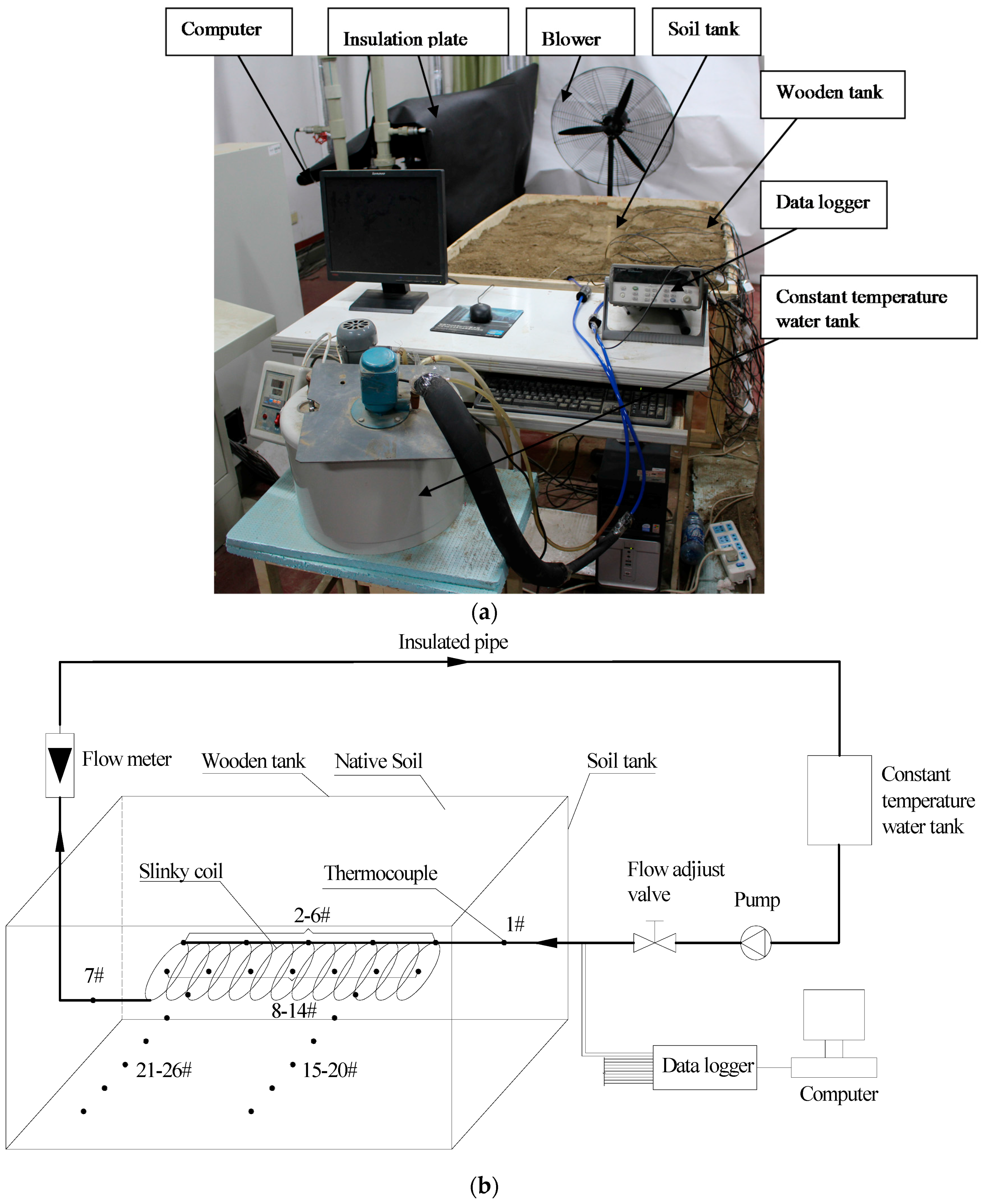
Figure 3.
Thermocouple arrangements in the slinky coil: (a) schematic diagram of thermocouples arrangement; and (b) picture of thermocouples locations.
Figure 3.
Thermocouple arrangements in the slinky coil: (a) schematic diagram of thermocouples arrangement; and (b) picture of thermocouples locations.

Figure 4.
Thermocouple arrangements in the soil surrounding the slinky coil: (a) schematic diagram of thermocouple arrangements in the soil; and (b) picture of thermocouples locations in the soil.
Figure 4.
Thermocouple arrangements in the soil surrounding the slinky coil: (a) schematic diagram of thermocouple arrangements in the soil; and (b) picture of thermocouples locations in the soil.
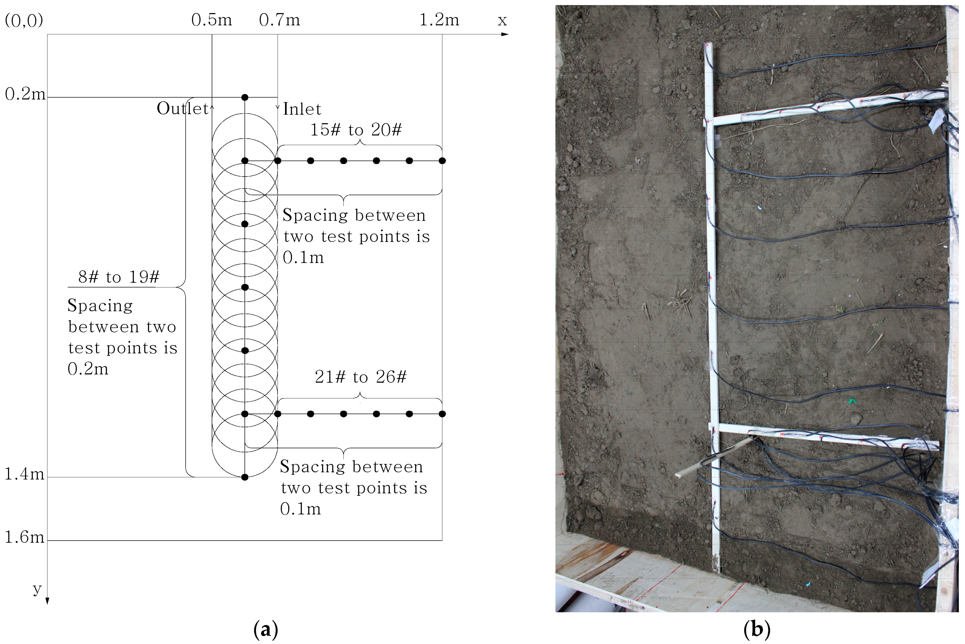
Figure 5.
Variation curves of heat release rate of slinky coil with time for different inlet temperatures.
Figure 5.
Variation curves of heat release rate of slinky coil with time for different inlet temperatures.
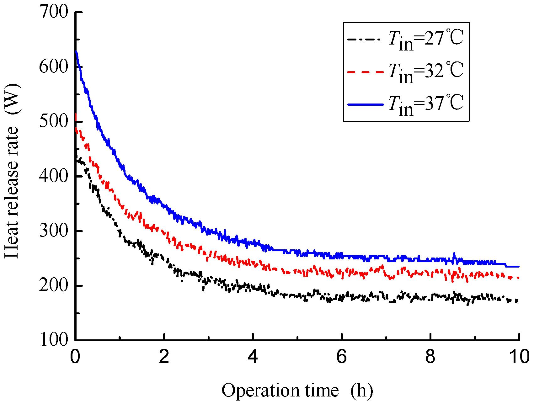
Figure 6.
Variation curves of soil excess temperature at different location with time for various inlet temperatures: (a) x = 0.6 m; and (b) x = 0.8 m.
Figure 6.
Variation curves of soil excess temperature at different location with time for various inlet temperatures: (a) x = 0.6 m; and (b) x = 0.8 m.

Figure 7.
Variation curves of heat release rate with time for different operation modes.

Figure 8.
Variation curves of soil excess temperature at x = 0.6 m and y = 0.4 m with time for different operation modes.
Figure 8.
Variation curves of soil excess temperature at x = 0.6 m and y = 0.4 m with time for different operation modes.
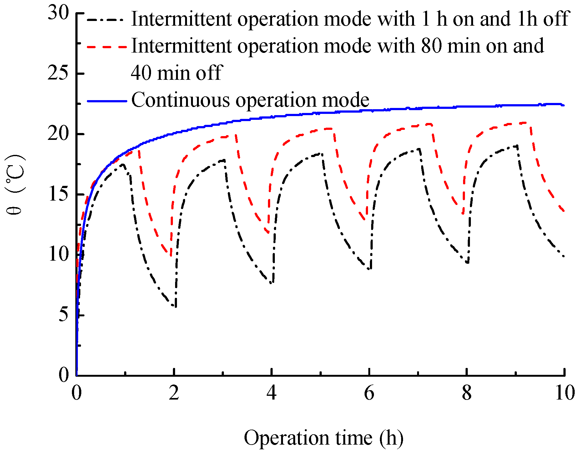
Figure 9.
Variation curves of heat release rate of coil with time for different coil central interval distances.
Figure 9.
Variation curves of heat release rate of coil with time for different coil central interval distances.

Figure 10.
Variation curves of heat release rate per unit length of the coil with time for different coil central interval distances.
Figure 10.
Variation curves of heat release rate per unit length of the coil with time for different coil central interval distances.
Figure 11.
Variation curves of soil excess temperature at x = 0.6 m and y = 0.2 m with time for different coil central interval distances.
Figure 11.
Variation curves of soil excess temperature at x = 0.6 m and y = 0.2 m with time for different coil central interval distances.
Figure 12.
Variation curves of heat release rate of the coil with time for different wind velocities.
Figure 12.
Variation curves of heat release rate of the coil with time for different wind velocities.

Figure 13.
The physical model of horizontal slinky coil ground heat exchanger: (a) equivalent straight pipe with same spacing; and (b) computation region for equivalent straight pipe.
Figure 13.
The physical model of horizontal slinky coil ground heat exchanger: (a) equivalent straight pipe with same spacing; and (b) computation region for equivalent straight pipe.

Figure 14.
Schematic of heat exchange of fluid inside coil for unit length of pipe.

Figure 15.
Comparison of heat release rate of coil between calculated value and experimental data: (a) comparison curves of heat release rate of coil for calculated and experimental values; and (b) calculation error analysis.
Figure 15.
Comparison of heat release rate of coil between calculated value and experimental data: (a) comparison curves of heat release rate of coil for calculated and experimental values; and (b) calculation error analysis.

Figure 16.
Soil temperature distribution after 45 days operation for different groundwater advection velocity: (a) u = 50 m/year; and (b) u = 300 m/year.
Figure 16.
Soil temperature distribution after 45 days operation for different groundwater advection velocity: (a) u = 50 m/year; and (b) u = 300 m/year.

Figure 17.
Variation curves of heat release rate with time for different groundwater advection velocities.
Figure 17.
Variation curves of heat release rate with time for different groundwater advection velocities.
Figure 18.
Variation curves of heat release rate with time for different soil types.
Figure 19.
Variation curves of water temperature along the pipe length at the end of 40 days operation for different soil types.
Figure 19.
Variation curves of water temperature along the pipe length at the end of 40 days operation for different soil types.
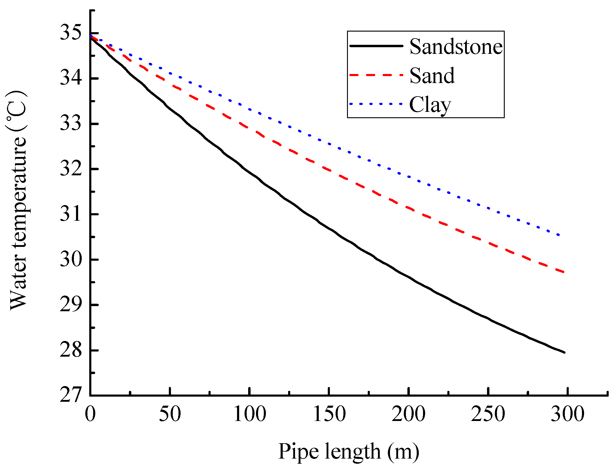
Figure 20.
Variation curves of energy released into ground with time for different buried depths.

Figure 21.
Variation curves of water temperature along the pipe length for different buried depths.

Table 1.
The main parameters for the model test system and physical prototype.
| Parameters | Central Distance/m | Coil Diameter/m | Inside Diameter of Coil/m | Flow Velocity/m/s | Re |
|---|---|---|---|---|---|
| Prototype | 0.2 | 1 | 0.025 | 0.12 | 3731 |
| Model | 0.04 | 0.2 | 0.005 | 0.6 | 3731 |
Table 2.
Errors of the main parameters in the experiment.
| Parameters | Type of Data | Typical Value | Unit | Relative Uncertainty |
|---|---|---|---|---|
| Average soil temperature | Measured | 28 | °C | 4.2% |
| Average inlet water temperature for the slinky coil | Measured | 32 | °C | 4.3% |
| Average outlet fluid temperature for the slinky coil | Measured | 27 | °C | 4.6% |
| Average flow rate of water | Measured | 0.04 | m3/h | 5.4% |
| Average heat release rate of coil | Calculated | 274 | W | 4.6% |
| Average heat flux per unit pipe length | Calculated | 16.5 | W/m | 4.4% |
| Average excess soil temperature | Calculated | 16 | °C | 4.7% |
Table 3.
Calculated conditions.
| Parameters | Value |
|---|---|
| Thermal conductivity of pipe, λp/W·m−1·K−1 | 0.48 |
| Inside diameter of equivalent pipe, din/m | 0.022 |
| Outside diameter of equivalent pipe, dout/m | 0.024 |
| Lp/Lt, n | 6 |
| Thermal conductivity of soil, λs/W·m−1·K−1 | 0.9 |
| Density of soil, ρs/kg·m−3 | 1500 |
| Specific heat of soil, cs/J·kg−1·K−1 | 1100 |
| Solar absorptivity, αs | 0.8 |
| Density of fluid, ρf /kg·m−3 | 1000 |
| Specific heat of fluid, cp/J·kg−1·K−1 | 4100 |
| Thermal conductivity of fluid, λf/W·m−1·K−1 | 0.56 |
| Flow rate, v/L·s−1 | 0.2 |
| Burial depth, zp/m | 2.4 |
| Length of trench, L/m | 50 |
| Width of computation region/m | 12 |
| Depth of computation region/m | 13 |
| Inlet water temperature of coil, Tin/°C | 35 |
| Mean ground temperature, TM/°C | 17.5 |
| Amplitude of annual temperature, A0/°C | 14.5 |
| Day from January 1st at which the minimum temperature occurs, τ0/day | 340 |
| Total operation time/day | 90 |
| Groundwater table/m | 2 |
| Porosity ε | 0.4 |
| Groundwater advection velocity, m·a−1 | 150 |
Table 4.
Thermal properties for three soil types.
| Soil Type | Density/kg/m3 | Specific Heat/J/(kg·K) | Thermal Conductivity/W/(m·K) | Thermal Diffusivity/m2/s |
|---|---|---|---|---|
| Clay | 1500 | 1100 | 0.9 | 0.545 × 10⁻⁶ |
| Sand | 2000 | 700 | 2.0 | 1.430 × 10⁻⁶ |
| Sandstone | 2500 | 1400 | 3.2 | 0.900 × 10⁻⁶ |
© 2017 by the authors. Licensee MDPI, Basel, Switzerland. This article is an open access article distributed under the terms and conditions of the Creative Commons Attribution (CC BY) license (http://creativecommons.org/licenses/by/4.0/).
Share and Cite
MDPI and ACS Style
Zhang, C.; Yang, W.; Yang, J.; Wu, S.; Chen, Y. Experimental Investigations and Numerical Simulation of Thermal Performance of a Horizontal Slinky-Coil Ground Heat Exchanger. Sustainability 2017, 9, 1362. https://doi.org/10.3390/su9081362
AMA Style
Zhang C, Yang W, Yang J, Wu S, Chen Y. Experimental Investigations and Numerical Simulation of Thermal Performance of a Horizontal Slinky-Coil Ground Heat Exchanger. Sustainability. 2017; 9(8):1362. https://doi.org/10.3390/su9081362
Chicago/Turabian StyleZhang, Chengbin, Weibo Yang, Jingjing Yang, Suchen Wu, and Yongping Chen. 2017. "Experimental Investigations and Numerical Simulation of Thermal Performance of a Horizontal Slinky-Coil Ground Heat Exchanger" Sustainability 9, no. 8: 1362. https://doi.org/10.3390/su9081362
Note that from the first issue of 2016, this journal uses article numbers instead of page numbers. See further details here.