Investigation of the Impacts of Urban Land Use Patterns on Energy Consumption in China: A Case Study of 20 Provincial Capital Cities


1
Huaihai Development Research Institute, Jiangsu Normal University, Heping Road 57, Xuzhou 221009, China
2
Institute of the Belt and Road, Jiangsu Normal University, Heping Road 57, Xuzhou 221009, China
3
Department of Spatial Information Management and Modelling, Faculty of Spatial Planning, TU Dortmund University, August-Schmidt-Str. 10, 44227 Dortmund, Germany
4
School of Resources and Geosciences, China University of Mining and Technology, Daxue Road 1, Xuzhou 221116, China
*
Author to whom correspondence should be addressed.
Sustainability 2017, 9(8), 1383; https://doi.org/10.3390/su9081383
Submission received: 28 June 2017
/
Revised: 26 July 2017
/
Accepted: 2 August 2017
/
Published: 7 August 2017
Abstract
:Urban land use patterns are increasingly recognized as significant contributors to energy consumption. However, few studies have quantified the impacts of urban land use patterns on energy consumption. In this study, we analyzed the impacts of urban land use patterns on energy consumption for 20 provincial capital cities in China from 2000 to 2010. Landsat data and spatial metrics were first used to quantify the urban land use patterns, and then city-level energy consumption was estimated based on nighttime light (NTL) data and statistical provincial energy consumption data. Finally, a panel data analysis was applied to investigate the impacts of urban land use patterns on energy consumption. Our results showed that NTL data were effective for estimating energy consumption at the city level and indicated that accelerated energy consumption was caused by increases in the irregularity of urban land forms and the expansion of urban land. Moreover, significant regional differences in the impacts of urban land use patterns on energy consumptions were identified. Our results provide insights into the relationship between urban growth and energy consumption and may support effective planning towards sustainable development.
1. Introduction
Significant climate change was observed worldwide in recent decades, and it represents a universal and important phenomenon [1], with global warming the most obvious climate change. As the center of human activities and socioeconomic development, urban land covers only 3% of the Earth’s land surface [2]; however, it is the greatest contributor to energy consumption [3]. In China, rapid urban development has resulted in considerable environmental challenges, including energy consumption [4], and the total energy consumption in China in 2010 was 3606.5 million tons of Standard Coal Equivalent (SCE), which exceeded that of the United States for the first time. Suppressing energy consumption in urban areas while maintaining rapid economic development is regarded as a key challenge for local governments [5].
In the context of this complex issue, formulating and implementing effective measures to promote energy efficiency to mitigate climate change has become increasingly urgent. Recent issues related to the analysis of the driving factors of climate change have attracted increasing attention. In addition to the traditional energy consumption reduction measures that depend on policy and technology, studies have also nominated the form of an urban landscape as one of the most important factors that contribute to energy consumption [4]. Numerous studies have identified factors that can be used to explain the relationship between energy consumption and urban form, especially in terms of the impact of urban forms on transportation [6], residential energy demand [7], and heat island effects [8]. Certain aspects of urban forms can greatly affect energy consumption, such as the size, pattern of mixing of land uses and pattern of travel [9]. Additionally, previous studies have indicated that a compact urban form can effectively reduce energy consumption. Compact and polycentric development patterns help reduce energy consumption [10]. The form of an urban landscape has an impact on the travel behavior and energy consumption of individuals while traveling [11]. Addressing sustainable urban forms, Ye et al. determined that compactness is positively linked with household energy consumption [12]. By selecting and analyzing the 125 largest urbanized areas in the U.S., Lee and Lee investigated how the urban form influences household energy consumption [13]; their results indicated that the reduction of energy consumption can be realized in terms of urban form optimization and urban planning. Previous studies have mainly analyzed energy consumption from the perspectives of transportation, household heating and electricity consumption. However, research has not been performed to explore the link between energy consumption and urban form from the perspective of land use patterns. Although previous studies can provide insights into how urban forms affect energy consumption, only a limited number of studies have quantitatively analyzed the impact of temporal changes in urban form on energy consumption.
Moreover, previous studies have mainly focused on exploring the relationships at the national level and have not considered regional differences. Therefore, the impacts of spatial heterogeneity may have been ignored, which could result in systematic bias in the exploration and analysis of the relationships [4] as well as inconsistent results that could not be explained [14]. Significant regional differences in urban development and urban land use patterns in China are related to its vast territory [15]. Limited empirical work has been conducted to establish or compare the magnitude of the impacts of urban land use patterns on energy consumption across regions while also considering spatial heterogeneity [14].
Estimating energy consumption at the city level is the first step to reducing energy consumption [16]. Meng et al. argued that our current understanding of urban energy consumption and related factors is largely limited by the absence of comprehensive data on urban energy consumption in developing countries [17]. This lack of data is also observed for China, where energy consumption data at the city level are difficult to obtain [18,19]. The nighttime light (NTL) data acquired from the Defense Meteorological Satellite Program/Operational Linescan System (DMSP/OLS) measures light on the Earth’s surface [20]. Several studies have proved that NTL data have informational value for countries that do not have consistent and accurate statistical data for monitoring socioeconomic activities and estimating socioeconomic data, such as population [21], income [22], gross domestic product (GDP) [23] and electricity consumption [24]. However, methods of estimating city-level energy consumption via NTL data have attracted little attention.
This study aims to estimate energy consumption at the city level and analyze the impact of urban land use patterns on energy consumption to support effective urban planning and policies to promote energy efficiency. For this purpose, variations in the urban land use patterns are derived and analyzed using remote sensing (RS) data and a series of spatial metrics. City-level energy consumption is then estimated using NTL data. Based on the calculated spatial metric values and estimated city-level energy consumption, a panel data analysis is conducted to investigate the impacts of urban land use patterns on energy consumption during the rapid urbanization process.
2. Materials and Methods
2.1. Study Area and Data
The 35 largest cities in China, including the capitals of each province and metropolis, contained only 18% of the total population but emitted 40% of CO2 in 2010 [4,25]. At present, the speed of development of certain province capitals has exceeded that of metropolises in China, such as Beijing and Shanghai. In addition to six municipalities and special administrative regions (Beijing, Chongqing, Hong Kong, Macau, Shanghai and Tianjin), the total number of province level cities in China is 28, which include 23 provincial capital cities and the capitals of China’s five autonomous regions. For this study, we selected the 20 provincial capital cities that constitute fast growth areas (Table 1), and their spatial distributions are presented in Figure 1.
The total population of the 20 cities was 50.00 million in 2000 and increased to 65.07 million in 2010. Additionally, the sum of the GDP of these 20 cities rapidly increased from 960.18 billion RMB to 4525.36 billion RMB from 2000–2010 [26]. Because of the imbalances in socioeconomic level and resource distribution among the cities, the regional characteristics of energy consumption also showed different patterns. According to the degree of socioeconomic development and geographical distribution, mainland China is divided into four major economic regions: the eastern region (Shijiazhuang, Jinan, Nanjing, Hangzhou, Fuzhou), the central region (Taiyuan, Zhengzhou, Hefei, Wuhan, Changsha), the western region (Yinchuan, Xining, Lanzhou, Xi’an, Kunming, Nanning) and the northeast region (Harbin, Changchun, Shenyang). This division can provide the basis for the development of regional development policies by the Chinese government.
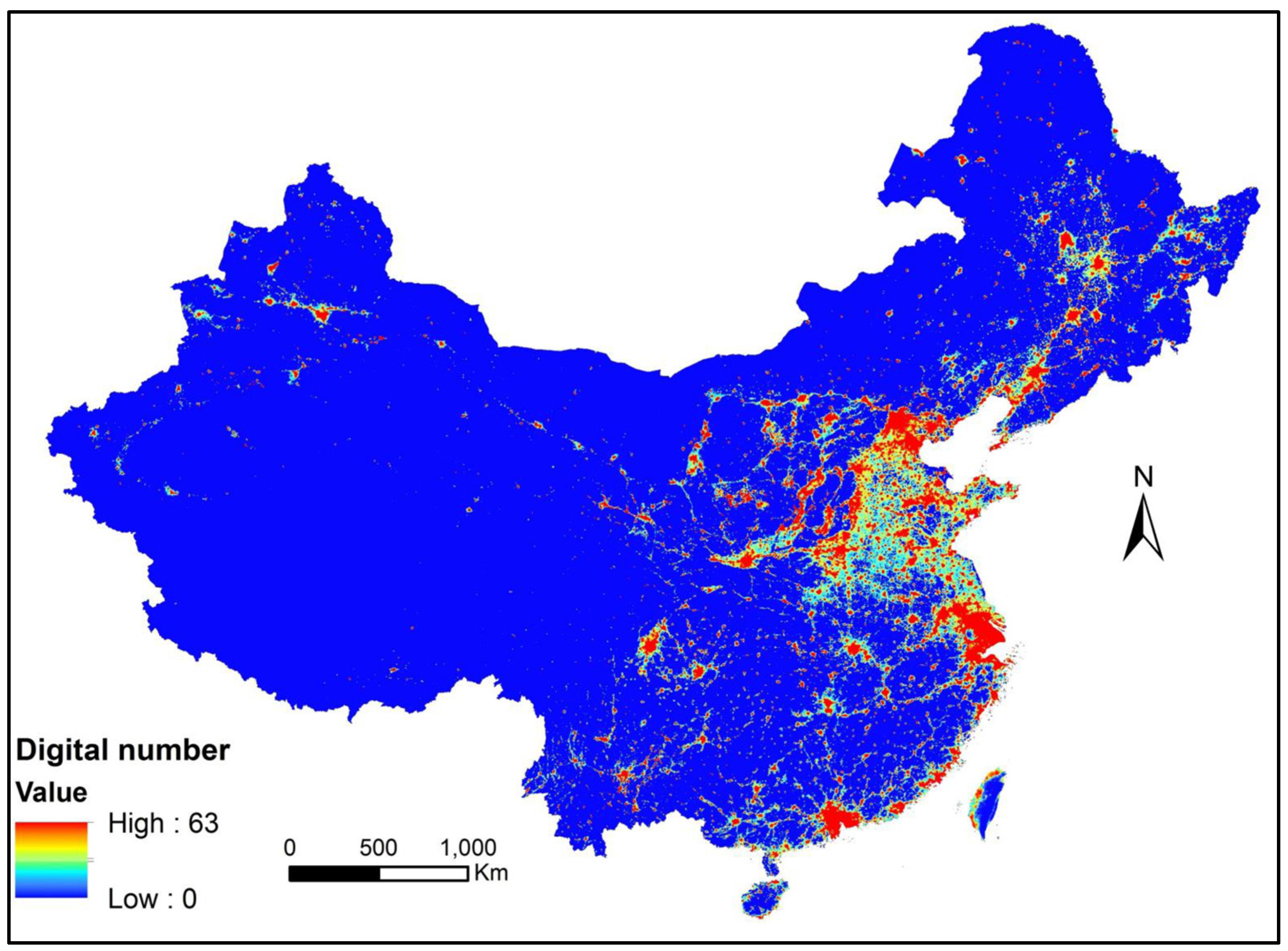
Landsat 5 TM images (U.S. Geological Survey) for 2000, 2003, 2006 and 2010 were acquired and used to analyze the dynamics of urban land cover. NTL data from DMSP/OLS were also used in this study. The OLS sensor is different from those used to detect ground objects based on the reflection characteristics of solar radiation. NTL data can capture the lights from cities, towns, and other sites with persistent lighting [27]. NTL data are one of the most important data sources for monitoring socioeconomic activity, and they present the global annual average brightness in units of a 6-bit digital number (DN) ranging from 0 (background) to 63 (brightest). The spatial resolution of NTL data is a 30 arc-second grid. Figure 2 shows the NTL data obtained from satellite F18 for China in 2010. The images of multi-temporal NTL data for the study period were acquired by four sensors: F14 (1999–2003), F15 (2000–2007), F16 (2004–2009), F18 (2010–2011).
Officially acquiring precise data was difficult because of the absence of city-level energy consumption data in China. A top-down method was adopted to downscale province energy consumption into city energy consumption (2000–2010) because only the annual energy consumption data at the province level (2000–2010) was available from the China Energy Statistical Yearbooks.
2.2. Spatial Metrics
The maximum likelihood classifier (MLC) was selected to classify the Landsat images into two categories: urban land and non-urban land. For each image, 100–120 training samples were adopted to train the image in order to ensure that all spectral classes covering urban and non-urban land were sufficiently represented in the training statistics. In order to assess the accuracy of classification map, a total of 200 random points generated by stratified random sampling method were used. Following the land cover classification, the quantification of urban land use patterns was conducted using a set of spatial metrics. Both complementarity and diversity are considered to provide deep insights into the characteristics of urban spatial patterns, and five metrics were chosen in the study from a large portfolio of partly redundant spatial metrics: CA (Class Area), which represented the total urban area in the study area; LPI (Largest Patch Index), which represented the largest urban patch divided by the total urban area (CA and LPI were used to describe the composition of the landscape); NP (Number of Patches), which represented the number of patches in the urban area; and ENN (Euclidean nearest-neighbor distance) and SHAPE (Shape index), which were used to describe the structure and configuration of the urban areas. To consider the different influence of patches according to the areas, ENN_AM (area-weighted mean Euclidean nearest-neighbor distance) and SHAPE_AM (area-weighted mean Euclidean nearest-neighbor distance) were calculated by incorporating weighting. ENN_AM is the area-weighted mean straight-line distance from one patch to the closest patch, and SHAPE_AM is the irregular degree of urban patches, and it increases when the patch shapes become more irregular [28].
2.3. Processing of NTL Data
Six satellites were used to produce NTL data from 1992 to 2013. However, strict intercalibration is not available for NTL data acquired by the different satellites [29]. Therefore, many inconsistent lit pixels are found in NTL data [30]. The cumulative DN values differ between two satellites for the same year. Additionally, the DN values acquired from the same satellite abnormally decrease with time. This phenomenon cannot accurately reflect the urban development process in developing countries, especially in China, which shows rapid development of urban socioeconomic conditions. Considering these shortcomings, continuity and comparability of NTL data must be promoted. In this study, the data were calibrated in three steps: intercalibration, intra-annual correction, and inter-annual correction. Intercalibration was conducted in this study to improve the continuity of NTL data for China from 2000 to 2010 based on the method developed by Elvidge et al. (2009) [29]. For the raw NTL data, the cumulative DN value in 2001 acquired from satellite F14 was 14,682,227 and the DN value from F15 was 17,153,402 (Figure 3a). Figure 3b shows that after conducting intercalibration, the corresponding DN values were 23,130,731 from F14 and 23,280,413 from F15.
Figure 3b shows that the cumulative DN values were different between two satellites for the same year. For the NTL data acquired from two satellites for the same year, the DN value of the corresponding pixel in the NTL image should be the same; otherwise, the pixel was defined as an unstable lit pixel. The intra-annual correction was conducted for NTL data in China using the information extracted from two different satellites for the same year to remove any intra-annual unstable lit pixels. The correction was conducted using Equations (1) and (2):
where is the DN value of the corrected unstable lit pixel i of the year n; and and indicate the DN value of the unstable lit pixel acquired from satellite a and satellite b, respectively. Figure 3c shows the cumulative DN value of NTL data after intra-annual correction.
Based on the characteristics of NTL data, the lit pixels detected in earlier NTL images should be maintained in later images. Additionally, the urban NTL would grow continuously over time because of the rapid urban growth in China. Therefore, the cumulative DN value of earlier NTL should not be larger than that of later NTL data. In the original NTL data, the cumulative DN value decreased with time; therefore, an inter-annual correction was applied to remove the inconsistencies of NTL data for the different years and to correct DN values for consistently lit pixels to ensure that the urban development processes in China were accurately depicted. The inter-annual correction was performed using the following equations:
where and represent the DN values of the lit pixel i in the years n and n − 1, respectively. If the DN value of a lit pixel in the early NTL image was larger than the DN value in the later NTL image, then the DN value was replaced by the DN value in the early NTL image; otherwise, the DN value was kept constant. As shown in Figure 3d, the variation trend of DN values maintained a continuous increase from 2000 to 2010 at an annual rate of increase of less than 15% after the inter-annual correction.
2.4. Estimation of Energy Consumption
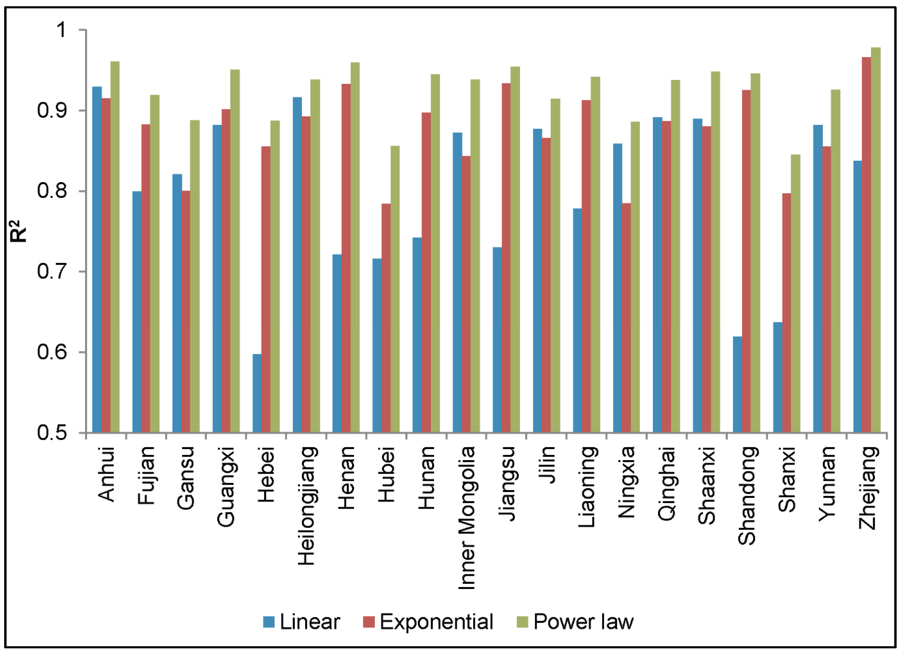
The main challenge for estimating city-level energy consumption by adopting NTL data is to quantify the relationship between the cumulative DN value of NTL data and the energy consumption within the specific area over time. In this study, the NTL data from 2000 to 2010 for 20 provinces were used. The available province energy consumption values were plotted against the cumulative DN values of NTL data within the specific province. Moreover, three statistical models (linear regression model, exponential regression model, and power law regression model) were applied to fit the energy consumption to the cumulative DN value of the calibrated NTL data over time (Equations (5)–(7)). The best-fitting regression model was identified and evaluated by comparing the R2 values of the three different regression models:
where is the provincial energy consumption and represents the cumulative DN value within the defined province p; and a and b are the parameters of the regression models.
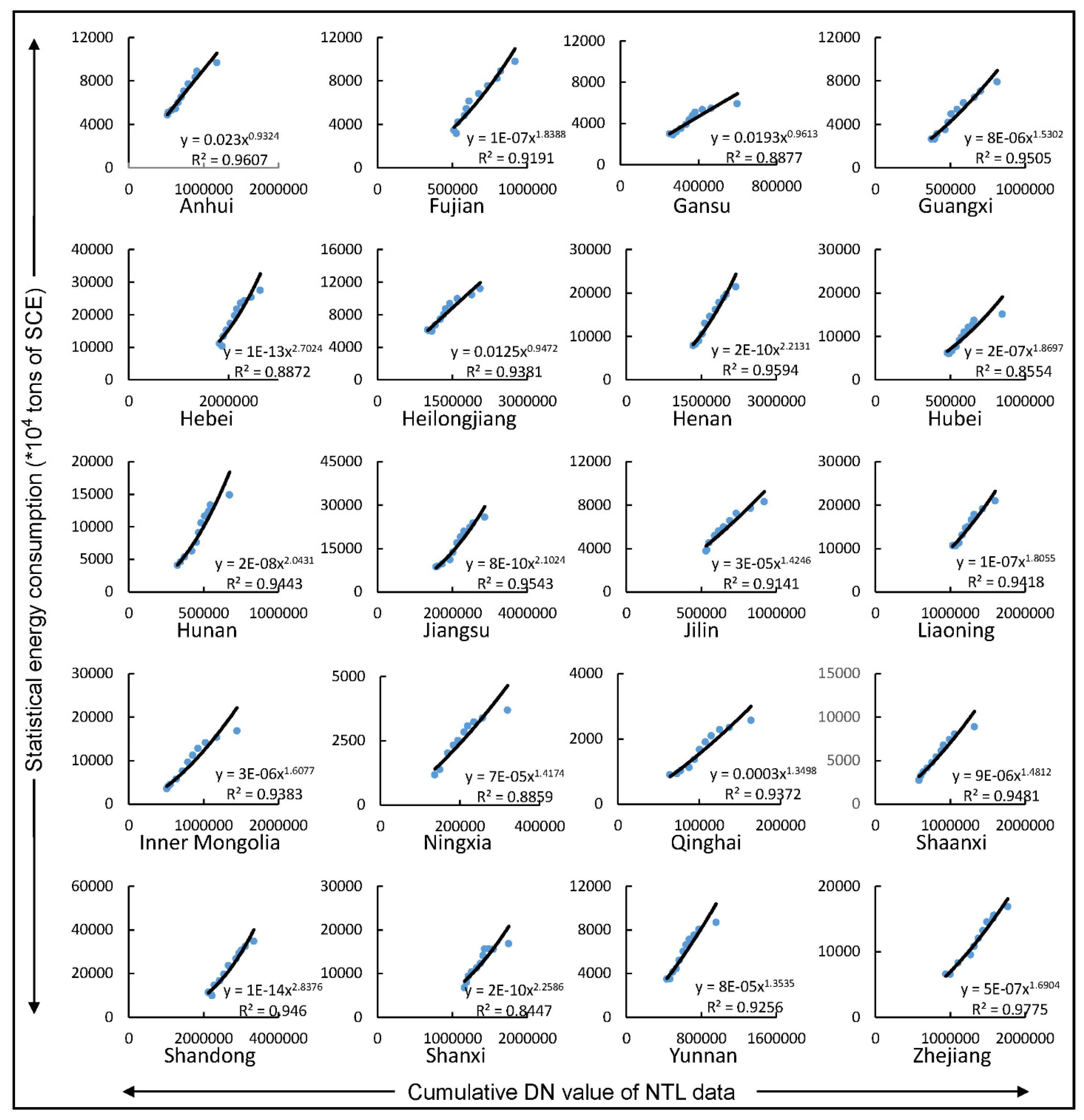
As shown in Figure 4, the power law regression was then used to downscale the provincial energy consumption to the city level. Figure 5 presents the scatter plots of cumulative DN values of NTL data and statistical energy consumption for the individual provinces.
The power law regression model for fitting energy consumption to NTL data is shown in Equation (8).
where a is the coefficient of the power law regression model; is the cumulative DN value of NTL data for province p in year t; and represents the estimated energy consumption for the province p in the year t.
To ensure that the estimated value was consistent with the statistical value, the relative error (Equation (9)) was used to correct the estimated value. The equation is expressed in Equation (10), which was generated by transforming Equation (8).
where is the relative error calculated by comparing the estimated energy consumption with the statistical energy consumption for province p in year t.
Equation (10) can be further transformed into the following equation:
where can be regarded as a new coefficient of the linear regression model at time t for a specific province. The coefficient indicates the energy consumption for a pixel with a DN value of 1, and it is not fixed and increases with the rise of cumulative DN value of NTL.
It was assumed that the relationship between DN value and energy consumption keeps constant within a certain province. Based on Equation (11), energy consumption can be estimated by Equation (12) for an individual city:
where is the energy consumption of city i. The coefficient varies over time and differs among provinces because of the regional differences involved in the characteristics of energy consumption. Energy consumption at the city level can be estimated using the variable-coefficient linear regression model.
2.5. Panel Data Analysis
A panel data analysis was conducted to explore the impacts of urban land use patterns on city-level energy consumption for 20 cities.
Normally, panel data analyses consist of three major types: pooled regression model (constant intercepts and constant coefficient), variable intercepts and constant coefficients model, and variable intercepts and variable coefficients model [31,32]. The specific formulas for these models can be described by Equations (13)–(15):
where i and t represent individuals and years; N and T are the total number of observed individuals and periods, respectively; and represent the independent and dependent variables, which were represented by the spatial metrics and city-level energy consumption in this study, respectively; is the error term, α denotes the intercepts, and β is the coefficient of the variable. In Equation (13), constant intercepts and coefficients indicate that there are no individual and structural changes in the regression model.
The variable intercepts and constant coefficients model is expressed by the following equation:
where represents the fixed effects or random effects.
In a fixed effects model, the intercept is uncorrelated with and a constant value for i, whereas for a random effects model is affected by involves not only a constant but also a random term caused by .
Moreover, variable coefficients can be denoted by as follows:
where represents the coefficient of explanatory variable , which can vary among individuals. This regression model implies that there are structural changes in addition to individual effects. can be specified as a fixed or random effect, such as the specification of
The panel data analysis is performed in three steps. The first step is to conduct an F-test. To avoid deviations in the models and improve the validity of parameter estimations, these two hypotheses are tested:
If is accepted, then the pooled regression model is more appropriate. If is rejected, the should be further tested. If is accepted, then the variable intercepts and constant coefficients model should be used; otherwise, both intercepts and coefficients are variable.
The F-test is conducted by comparing the Residual Sum of Squares (RSS) values of Equations (13)–(15):
where is the statistic for , in which both the coefficient and intercept remain constant for all individuals; is the statistic for , in which the coefficients are constant and intercepts are variable; , , and are the RSS values of Equations (15), (14) and (13), respectively; K represents the total number of explanatory variables; N represents the number of individuals; T denotes the number of periods. If is less than the critical value, then is accepted; otherwise, should be further tested. If is less than the critical value, then is accepted; otherwise, the variable intercepts and coefficients model should be used [33].
In this study, the value of T was 4. Considering the condition that T > K + 1 in the panel data model, T and K represent the number of time points and the independent variable, respectively. Therefore, the maximum value of K should be 2, which indicates that the regression model has at most two independent variables. All five metrics cannot be involved in one regression model because of this condition. Therefore, these metrics can be divided into several groups. Each group should include two metrics with a low correlation. Prior to estimating the parameters of the panel data model, Pearson’s correlation analysis was implemented to test the correlation among the metrics and select the combination of non-correlated metrics in each estimated model.
Then, if the F-test results indicated that both coefficients and intercepts were not constant, then the Hausman test was conducted to determine whether fixed or random effects will be used [34,35]:
where and are values generated from the fixed effect model and the random effect model, respectively; k represents the degree of freedom; and W represents the Wald statistics value. If W is zero, then the random effect model will be adopted; otherwise, the fixed effect model will be adopted.
3. Results and Discussion
3.1. Quantification of Urban Land Use Patterns
The urban land use accuracies of all study images were over 90%. Therefore, the classified maps could be used for further analysis. Figure 6 shows the spatial patterns of urban expansion for the periods 2000–2003, 2003–2006, and 2006–2010. The urban growth detection process clearly identified the dynamic development path of the urban areas during the study period.
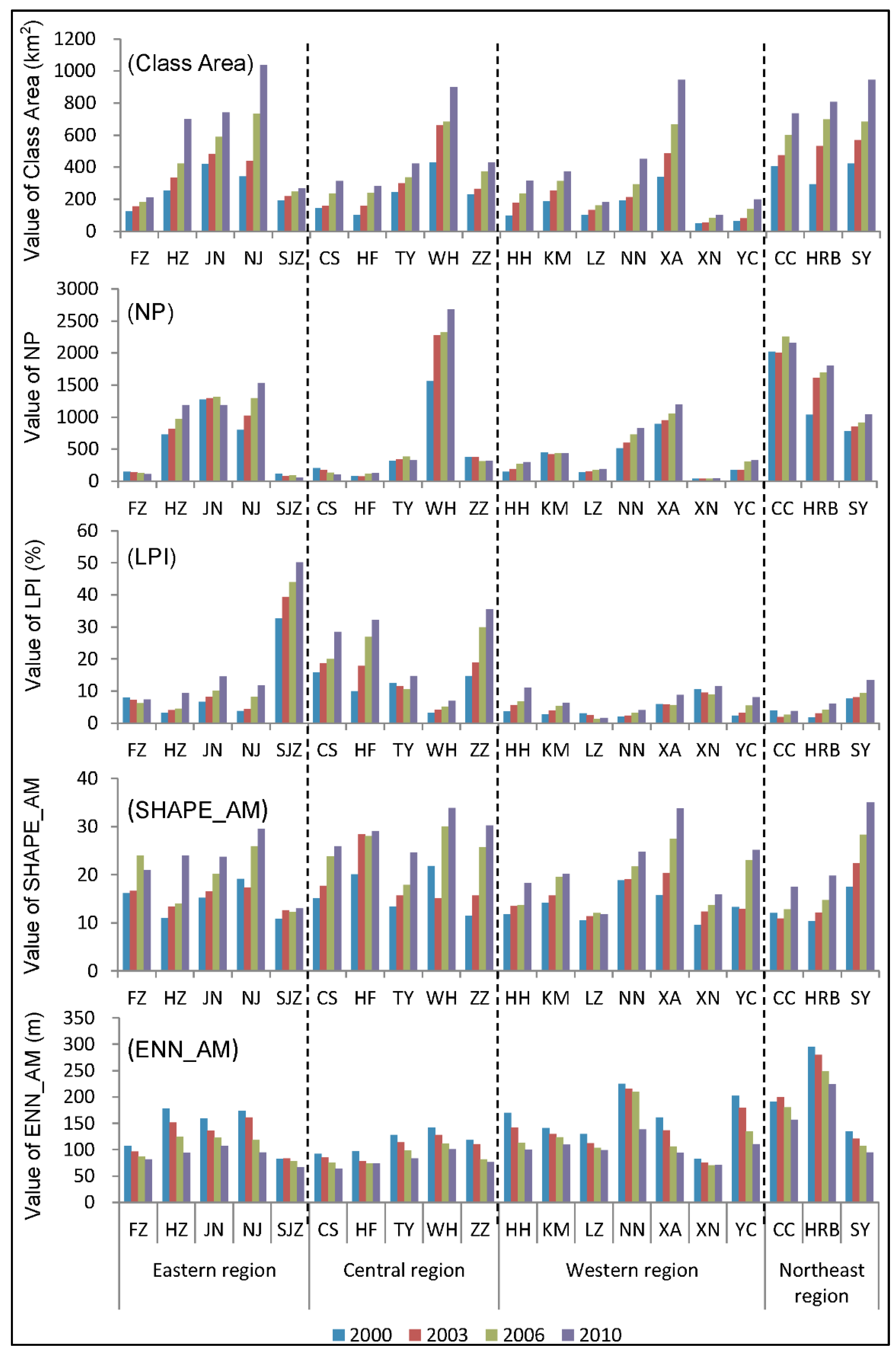
Figure 7 shows the calculated spatial metrics for the 20 cities in 2000, 2003, 2006 and 2010. The results indicate the remarkable differences in the change trends and magnitudes of the metrics among the cities. The CA value rapidly increased in four different regions during the study period. A higher average value of urban area was found in the eastern and northeastern regions than in the two other regions, which can be attributed to the rapid economic development in the eastern and northeastern regions.
As shown in Figure 7, variations in both the NP and NTL values were found in the 20 cities during the study period. The increased NTL reflected the historical growth of city cores. The allocation of new urban areas consisted of the outward development from the original city center and the growth of new urban patches, which are illustrated by increases in both the NTL and NP values. A slight increase in the NP value was found in the central and western regions except for Wuhan City. However, inverse trends occurred in certain eastern and northeastern cities. Many patches were developed for industrial development and infrastructure construction. As a special case, Wuhan experienced a dramatic increase in NP values and achieved the highest NP value in 2010, whereas a relatively lower LPI value was found in 2010. Compared with Wuhan, Shijiazhuang in the eastern region had the highest LPI value of 50.176 and a lower NP value of 53.
The SHAPE_AM metric measures the compactness of an urban spatial pattern. As the rapid urbanization proceeded, the diffuse sprawling development of the studied cities was illustrated by the continuous increases in SHAPE_AM.
The ENN_AM value decreased in all cities, which indicated that the urban patches became more proximate. The distance between patches decreased as the urban patches became larger. Additionally, the small patches were more connected with central urban patches, which can be confirmed by the decreasing ENN_AM values, and these changes could result in the loss of open space between the urban patches. As evidenced by Figure 6, the vacant land between patches was filled by newly developed land, and new urban patches were found very close to the urban patches.
3.2. Urban Energy Consumption
The energy consumption for 20 cities was estimated using Equation (12). The parameters are listed as following (Table 2).
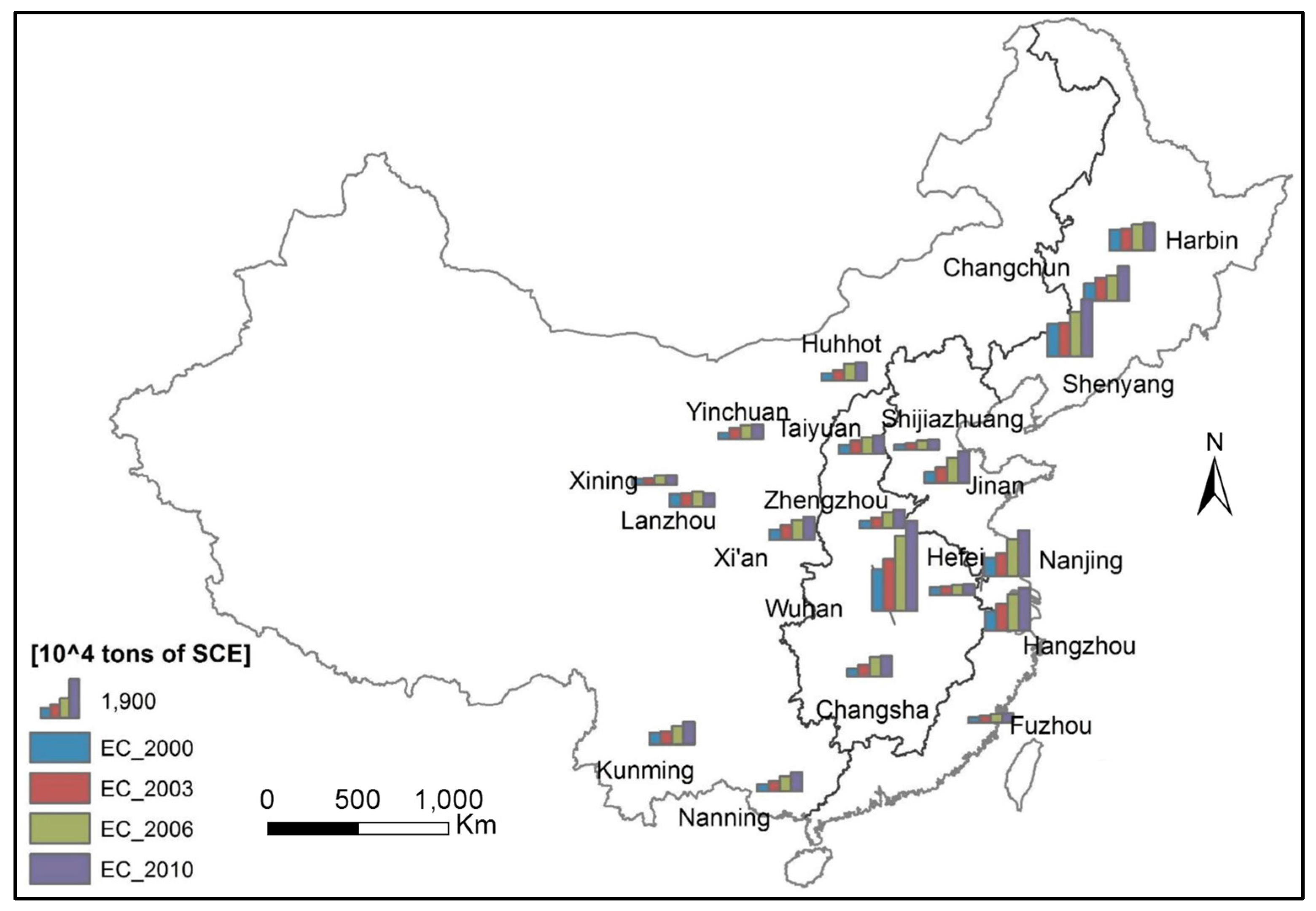
Figure 8 presents the estimated energy consumption values in 20 cities from 2000 to 2010 and indicates that the energy consumption of each city gradually increased during the period. The sum of energy consumption of the 20 cities grew by approximately 102% from 10,902.89 × 104 tons in 2000 to 22,121.36 × 104 tons of SCE in 2010. In Jinan, energy consumption rose by approximately two fold from 2000 to 2010, which was the highest rate of increase among the 20 cities. Wuhan was found to be the largest energy consumer, and its energy consumption dramatically rose from 1708.09 × 104 tons in 2000 to 3702.64 × 104 tons of SCE in 2010.
3.3. Exploration of the Impacts of Urban Land Use Spatial Patterns on Energy Consumption
To examine the links between urban spatial patterns and energy consumption, the estimated urban energy consumption served as the dependent variable and spatial metric values served as the independent variable. The impacts of urban land use spatial pattern on energy consumption were investigated using panel data models.
Table 3 presents the correlations among the spatial metrics in the study. Based on the calculated correlation coefficients, four pairs of metrics met the requirement: CA and LPI (Model 1); CA and ENN_AM (Model 2); NP and SHAPE_AM (Model 3); and LPI and SHAPE_AM (Model 4). The four combinations of metrics were adopted to build four regression models.
Table 4 demonstrated that the variable intercepts and constant coefficients model should be adopted for these four models. The results of the Hausman test (Table 5) showed that the fixed effect model was selected for further analyses.
The test results indicated that a relationship occurred between the spatial metrics and energy consumption as follows:
where is the energy consumption of city i; is the city fixed coefficient; and represent the two spatial metrics for city i at time t; and are the coefficients of the selected spatial metrics; and is the error term.
Four fixed effect models for estimating the overall energy consumption were estimated based on the four different combinations of spatial metrics (Table 6). The first model examined the effect of the composition of CA and LPI on energy consumption. Similarly, the other three models investigated the effects of the composition of CA and ENN_AM, NP and SHAPE_AM, and LPI and SHAPE_AM on energy consumption. The parameters of the relationship between energy consumption and urban spatial pattern were estimated using the panel data analysis. The variable coefficients results showed that urban spatial patterns had important but different impacts on energy consumption, and all coefficients were significant at the level of 1%. Therefore, all selected spatial metrics were significantly correlated with energy consumption. CA, NP, LPI, and SHAPE_AM had positive relationships with energy consumption (the coefficient of LPI was negative in Model 4 but was not significant), whereas ENN_AM was negatively correlated with city-level energy consumption.
The positive correlation between CA and overall energy consumption indicated that urban expansion was related to the increased energy consumption, which is consistent with the widely known relationship between urban area and energy consumption in other investigation areas [36]. The positive relationship can be explained from the perspective of population growth and economic development [37]. The increase in population, which is the main driver of urban growth, was responsible for the increase in energy consumption. Along with the dramatic urbanization process in China, individuals migrating from rural areas to urban areas accounted for the greatest contribution to the significant population growth in urban areas. The new urban migrants consumed greater energy per capita than their rural settlements. A large percentage of energy supply in rural areas relies on biomass, whereas urban energy consumption is primarily derived from commercial fuels. Additionally, the change in the lifestyle of migrants because of the rural-to-urban migration would cause changes in the typical energy consumption profile of these migrants [38]. The socioeconomic activities of rural-to-urban migrants shifted from agricultural to service, construction, and industrial activities, which have significantly different energy intensities compared with agricultural activities in rural areas.
The rapid economic development also contributed to the dramatic urban expansion. In China, manufacturing industries are commonly characterized as having low energy efficiency and high labor intensity and normally play an important role in the regional economy of most cities in China [39], in which more energy-consuming sectors are concentrated in urban areas. Therefore, the development of regional economies should be the one of the most important factors influencing the increase of energy consumption. Moreover, rising incomes make the lifestyles of urban residents more energy intensive [25]. China will face a huge challenge if urban expansion in the future remains at a high rate.
As indicated by the estimated results, NP had a significantly positive effect on energy consumption. Massive construction formed many new urban patches, which represented a crucial contributor to the rapid growth of urban areas. The development of new urban patches may lead to the accelerated development of private and public transport, which requires more energy. Private transport significantly increases because of the newly developed patches [40]. For example, the scatter pattern of working and residential areas leads to long traveling distances between residences and work places [41]. Additionally, the new urban patches require more public infrastructure than the development within existing urban patches. The energy consumption could increase because of the construction and maintenance of the infrastructure [4]. Consequently, the growth in NP could have resulted in increased energy consumption.
SHAPE_AM represents the jaggedness of the shape of the patches. As indicated by Table 6, SHAPE_AM had a significant positive impact on energy consumption, which is consistent with the results of previous studies [42,43]. A compact urban pattern has been suggested to promote sustainable development because of the increased accessibility and reduced travel distance and the regeneration of urban areas [44,45].
LPI had a significant positive impact on the overall energy consumption. Compared with previous studies [34], our results indicated that the overall energy consumption would decrease with the growth of the percentage of the largest urban patches (the city core). Many researchers believe that compact cities have environmental, social and fiscal advantages and result in energy conservation [45]. To some degree, the negative relationship between LPI and energy consumption suggests that compact urban patterns are correlated with less energy consumption. However, the traffic congestion associated with compact cities, which has been ignored by previous studies, has become a serious problem for the reduction of energy consumption. Traffic congestion is commonly characterized by longer trip times, lower speeds, and increased vehicular queuing [46]. Moreover, because larger city cores provide a greater number of functions, activities would be concentrated in these areas [47]. However, larger city cores could result in traffic congestion because of the high settlement density and insufficient road resources. Therefore, traffic congestion plays a significant role in rising energy consumption. Additionally, Makido et al. concluded that the monocentric urban pattern with high density settlements may lead to high energy consumption [43]. Accordingly, the development of polycentric urban patterns can decrease energy consumption.
One interesting finding was the negative correlation between ENN_AM and energy consumption, which differs from the results of previous studies. Yin et al. noted that decreased distances to a city center were the most influential factor for improving energy efficiency in the Kumamoto metropolitan area [48]. Chen et al. argued that ENN_MN had a positive correlation with energy consumption in the Pearl River Delta [34]. In this study, ENN_MN was replaced by ENN_AM, which averaged the distances by weighting patch areas so that smaller patches weighed less than larger patches. This weighting improved the measure of ENN_MN at the global level because the generation of smaller patches showed a stronger correlation with image pixel size than natural or artificial objects [49], which may have been one of the reasons for the different correlation results. Moreover, the increased number of private cars may primarily explain the different correlation results because the number of cars increases along with the increases in income and changes in lifestyles. Therefore, the potential traffic for shopping and leisure activities will increase when the spatial connection between relatively smaller patches and city cores is strong because additional energy will be consumed by the increased travel distances. Such changes are particularly obvious in fast-developing regions with many new residential areas built within new urban patches that are distant from the city core. The roads that connect new patches with the city core are constructed after new residential areas are constructed. However, if facilities such as hospitals, schools and markets are not included in such construction, then the residents must travel long distances between the city center, where these facilities are located, and their residences to access these service facilities.
Considering regional differences, the same procedure was performed to investigate the impacts of urban spatial patterns on energy consumption for the cities in the eastern, central, western, and northeast regions. The estimated parameters for the four regions are listed in Table 7, Table 8, Table 9 and Table 10. As shown in these tables, the spatial metrics (CA, NP, LPI, SHAPE_AM) were significantly related to energy consumption at the level of 5% or less in the eastern, central, and western regions. The coefficient of ENN_AM was significant in the western and eastern regions but was not significant at the level of 5% in the central region, which means that the rising energy consumption could not be explained by the variation of ENN_AM value. Additionally, because of the limited samples in the northeast region, only CA and LPI had significant correlations with energy consumption.
Focusing on the four regions, certain estimated coefficients suggested that the estimated outputs were consistent with the results generated by the models at the national level. Moreover, note that the impact of the spatial pattern on city level energy consumption varied spatially as exemplified by the impact of increasing urban land area on energy consumption, which had the greatest effect in the central region, followed by the eastern, western and northeast regions. The increased urban land area in the central region was mainly attributed to the rapid development of industries with high energy intensity, which would result in the rapid rise in energy consumption.
Additionally, the results showed that the impacts of other spatial pattern metrics on city level energy consumption were also variable. With an increase in the SHAPE_AM value of 1 in Model 3, the energy consumption in the eastern, central, and western regions increased by 41.8031 × 10⁴, 36.1556 × 10⁴, and 14.2506 × 10⁴ tons of SCE, respectively. The effect of urban pattern compactness in the eastern region was more marked than that in the other regions. Moreover, the impact of NP on urban energy consumption in the central region was more significant than that in the other regions.
The impact of LPI on energy consumption was positive in the eastern, western, and northeast regions, whereas it was negative in the central region. This regional difference could be attributed to differences in the economic and infrastructure levels among the different regions. The cities in the eastern and northeast regions are characterized by rapid urbanization and economic development as well as high population density. Although the relatively complete infrastructure and transportation system in a city core provides good opportunities for development, the rapidly increasing number of private cars could cause serious congestion. In the western region, the transportation system is not complete because of the relatively lower economic level. Therefore, congestion is also significant. However, congestion is not as serious in the central region as it is in other regions.
4. Conclusions
4.1. Methodology Implications
Compared with other satellite images used to monitor land cover and land use, NTL data can be quantitatively related to variations in socioeconomic activities [21]. This study developed a new method of estimating city-level energy consumption using NTL data. The accuracy of estimated energy consumption was improved by implementing the following three steps: (1) preprocessing of NTL data, (2) exploring the quantitative relationships between the province energy consumptions and NTL data using different regression models, and (3) estimating city-level energy consumption based on the corresponding correlations between NTL data and province energy consumption. The study proposed three steps for systematically correcting NTL data to improve continuity and comparability: intercalibration, intra-annual correction, and inter-annual correction. The results suggested that the abnormal discrepancies of NTL data can be greatly reduced by applying these corrections. Additionally, the challenge in estimating energy consumption using NTL data is to identify the correlation between pixel values and energy consumption over time. Three different regression models (linear, exponential, and power law) were applied to fit the response of NTL to energy consumption over time considering the regional differences. The best-fitting model for performing correlations was obtained by comparing the R2 values. The validation results implied that the identified model can be adopted to effectively estimate the energy consumption of a province. Moreover, the NTL data represented a suitable proxy for energy consumption in China. Compared with the unique models proposed in previous studies, different models were proposed to estimate urban energy consumption by considering the regional differences among 20 provinces. Focusing on each study area, this study proposed a variable-coefficient linear regression model by modifying the identified regression models within the specific province, and this approach was able to avoid the underestimations or overestimations of energy consumption observed in previous studies. Additionally, this study extended the work of previous studies by investigating the quantitative correlation between city-level energy consumption and urban land use patterns by considering the spatially varying effects of urbanization instead of global effects. Although spatial heterogeneity is not normally considered by independent variables, it may contribute to variations in the correlations among individuals. The varying intercepts and coefficients in the panel data analysis could solve this problem.
Although the significant correlation between NTL and energy consumption was revealed, the ability of NTL data can be limited due to the over-saturation of data value. In this study, we ignored the saturation effects when the NTL statistics were calculated. We assumed that there would be low or no change in the NTL brightness once an area's brightness reaches certain level. This assumption may be true in most areas, but can be problematic. Some studies have proposed different methods to correct the over-saturation effects of NTL data. However, over-saturation can still remain an issue because the existing methods are only suitable for a certain city. It would be valuable to conduct the over-saturation correction on the national scale or province scale in the further study.
4.2. Development Recommendations
In the context of rapid urbanization, developing and implementing a strict policy of controlling the rapid expansion of urban areas in certain cities is becoming increasingly important. The findings indicate that the growth of urban land areas is the major driver for the tremendous increase in energy consumption during the study period. Moreover, decelerating the economic growth process could be the most effective method of reducing energy consumption and mitigating global climate change. However, rapid economic growth and urbanization are currently the main goals of the Chinese government [50]. Therefore, the government faces the arduous challenge of continuously balancing increases in urban energy consumption and rapid economic growth with meeting environmental goals [25]. Urbanization significantly promotes urban growth but also results in more fragmented and irregular spatial patterns. The government should strive to optimize the urban spatial pattern to reduce energy consumption because irregular patterns contribute to the growth of energy consumption. Future urban development strategies that consider urban shape complexity should be designed. The coefficient estimated from the panel data analysis for 20 cities was 31.2928, which indicates that higher energy consumption efficiency can be realized when cities become more compact. This knowledge can help decision makers address methods of reducing energy consumption and achieving sustainable development. However, as indicated by the negative impact of LPI on energy consumption (−22.5420), certain environmental problems caused by compact cities may occur when development is only concentrated within a single city core, which could trigger longer travel distances and traffic congestion in the city core. Although most people are concentrated within city cores, individuals living in fringe or suburban areas must travel far to obtain the available services in the city cores. Therefore, it is necessary to avoid higher LPI value in designing urban land use pattern.
Moreover, policy measures for conserving energy should be adjusted to local conditions in China. Despite the significant increases in energy consumption found in all cities in this study, the growth rates of energy consumption varied across regions. Additionally, the panel data analysis showed that differences occurred among the different regions in terms of the urban spatial patterns and their impacts on energy consumption. Increases in urban land in the central region had the greater impact on urban energy consumption than those in other regions. The impact of increasing NP values in the eastern region was not as strong as that in other regions because the urban infrastructure and road system was more advanced than that of other regions. Therefore, planning and land use management should consider regional characteristics to lessen regional disparities and realize balanced development.
Supplementary Materials
The following are available online at www.mdpi.com/2071-1050/9/8/1383/s1, Table S1: The spatial metrics values of the 20 cities from 2000 to 2010, Table S2: The energy consumption for 20 provinces from 2000 to 2010 (Unit: 104 tons of SCE), Table S3: The cumulative DN values of NTL data for each province from 2000 to 2010, Table S4: The cumulative DN values of NTL data for each city from 2000 to 2010, Table S5: The estimated urban energy consumption from 2000 to 2010 (Unit: 104 tons of SCE).
Acknowledgments
This study was supported by the Scientific Research Foundation of Jiangsu Normal University (Grant No. 16XWR017), Priority Academic Program Development of Jiangsu Higher Education Institutions (PAPD): Regional New-type Urbanization Development, Jiangsu Research Base of Philosophy and Social Science: Jiangsu Research Base of Huaihai Development, Jiangsu Research Base of Decision Consulting: Jiangsu Research Base of Regional Coordinated Development.
Author Contributions
Jie Zhao analyzed the data; Jie Zhao, Nguyen Xuan Thinh, and Cheng Li wrote the paper.
Conflicts of Interest
The authors declare no conflict of interest.
References
- Zhou, X.Y.; Zhang, J.; Li, J.P. Industrial structural transformation and carbon dioxide emissions in China. Energy Policy 2013, 57, 43–51. [Google Scholar] [CrossRef]
- Dewan, A.W.; Yamaguchi, Y. Land use and land cover change in Greater Dhaka, Bangladesh: Using remote sensing to promote sustainable urbanization. Appl. Geogr. 2009, 29, 390–401. [Google Scholar] [CrossRef]
- Kennedy, C.; Steinberger, J.; Gasson, B.; Hansen, Y.; Hillman, T.; Havránek, M.; Pataki, D.; Phdungsilp, A. Methoology for inventorying greenhouse gas emissions from global cities. Energy Policy 2010, 38, 4828–4837. [Google Scholar] [CrossRef]
- Zhang, C.; Lin, Y. Panel estimation for urbanization, energy consumption and CO2 emissions: A regional analysis in China. Energy Policy 2012, 49, 488–498. [Google Scholar] [CrossRef]
- Wang, S.; Fang, C.; Wang, Y.; Huang, Y.; Ma, H. Quantifying the relationship between urban development intensity and carbon dioxide emissions using a panel data analysis. Ecol. Indic. 2014, 49, 121–131. [Google Scholar] [CrossRef]
- Hankey, S.; Marshall, J.D. Impacts of urban form on future US passenger-vehicle greenhouse gas emissions. Energy Policy 2010, 38, 4880–4887. [Google Scholar] [CrossRef]
- Liu, X.C.; Sweeney, J. Modelling the impact of urban form on household energy demand and related CO2 emissions in the Greater Dublin Region. Energy Policy 2012, 46, 359–369. [Google Scholar] [CrossRef]
- Stone, B.; Rodgers, M.O. Urban form and thermal efficiency: How the design of cities influences the urban heat island effect. J. Am. Plan. Assoc. 2001, 67, 186–198. [Google Scholar] [CrossRef]
- Owens, S.E. Energy, Planning and Urban Form; Pion: London, UK, 1986. [Google Scholar]
- Ou, J.P.; Liu, X.P.; Li, X.; Chen, Y.M. Quantifying the relationship between urban forms and carbon emissions using panel data analysis. Landsc. Ecol. 2013, 28, 1889–1907. [Google Scholar] [CrossRef]
- Ma, J.; Liu, Z.L.; Chai, Y.W. The impact of urban form on CO2 emission from work and non-work trips: The case of Beijing, China. Habitat Int. 2015, 47, 1–10. [Google Scholar] [CrossRef]
- Ye, H.; He, X.Y.; Song, Y.; Li, X.H.; Zhang, G.Q.; Lin, T.; Xiao, L. A sustainable urban form: The challenges of compactness from the viewpoint of energy consumption and carbon emission. Energy Build. 2015, 93, 90–98. [Google Scholar] [CrossRef]
- Lee, S.; Lee, B. The influence of urban form on GHG emissions in the US household sector. Energy Policy 2014, 68, 534–549. [Google Scholar] [CrossRef]
- Brunnermeier, S.B.; Levinson, A. Examining the evidence on environmental regulations and industry location. J. Environ. Dev. 2004, 13, 6–41. [Google Scholar] [CrossRef]
- Shen, L.; Cheng, S.; Gunson, A.J.; Wan, H. Urbanization, sustainability and the utilization of energy and mineral resources in China. Cities 2005, 22, 287–302. [Google Scholar] [CrossRef]
- Li, Y.; Li, Y.; Zhou, Y.; Shi, Y.; Zhu, X. Investigation of a coupling model of coordination between urbanization and the environment. J. Environ. Manag. 2012, 98, 127–133. [Google Scholar] [CrossRef] [PubMed]
- Meng, L.; Crijns-graus, W.H.; Worrell, E.; Huang, B. Estimating CO2 (carbon dioxide) emissions at urban sales by DMSP/OLS (Defense Meteorological Satellite Program’s Operational Linescan System) nighttime light imagery: Methodological challenges and a case study for China. Energy 2014, 71, 468–478. [Google Scholar] [CrossRef]
- International Energy Agency (IEA). World Energy Outlook 2008; International Energy Agency: Paris, France, 2008. [Google Scholar]
- Xie, Y.; Weng, Q. Detecting urban-scale dynamics of electricity consumption at Chinese cities using time-series DMSP-OLS (Defense Meteorological Satellite Program-Operational Linescan System) nighttime light imageries. Energy 2016, 100, 177–189. [Google Scholar] [CrossRef]
- Zhang, Q.; Schaaf, C.; Seto, K.C. The vegetation adjusted NTL urban index: A new approach to reduce saturation and increase variation in nighttime luminosity. Remote Sens. Environ. 2013, 129, 32–41. [Google Scholar] [CrossRef]
- Doll, C.H.N.; Pachauri, S. Estimating rural populations without access to electricity in developing countries through night-time light satellite imagery. Energy Policy 2010, 38, 5661–5670. [Google Scholar] [CrossRef]
- Chen, X.; Nordhaus, W.D. Using luminosity data as a proxy for economic statistics. Proc. Natl. Acad. Sci. USA 2011, 108, 8589–8594. [Google Scholar] [CrossRef] [PubMed]
- Wu, J.; Wang, Z.; Li, W.; Peng, J. Exploring factors affecting the relationship between light consumption and GDP based on DMSP/OLS nighttime satellite imagery. Remote Sens. Environ. 2013, 134, 111–119. [Google Scholar] [CrossRef]
- Letu, H.; Hara, M.; Yagi, H.; Naoki, K.; Tana, G.; Nishio, F.; Shuhei, O. Estimating energy consumption from night-time DMSP/OLS imagery after correcting for saturation effects. Int. J. Remote Sens. 2010, 31, 4443–4458. [Google Scholar] [CrossRef]
- Dhakal, S. Urban energy use and carbon emissions from cities in China and policy implications. Energy Policy 2009, 37, 4208–4219. [Google Scholar] [CrossRef]
- China National Bureau of Statistics. China City Statistical Yearbook 2001–2011; China Statistic Press: Beijing, China, 2011.
- Elvidge, C.D.; Baugh, K.E.; Dietz, J.B.; Bland, T.; Sutton, P.C. Radiance Calibration of DMSP-OLS Low-Light Imaging Data of Human Settlements. Remote Sens. Environ. 1999, 68, 77–88. [Google Scholar] [CrossRef]
- McGarigal, K.; Cushman, S.A.; Ene, E. FRAGSTATS v4: Spatial Pattern Analysis Program for Categorical and Continuous Maps. Computer Software Program Produced by the Authors at the University of Massachusetts, Amherst. Available online: http://www.umass.edu/landeco/research/fragstats/fragstats.html (accessed on 4 March 2015).
- Elvidge, C.D.; Ziskin, D.; Baugh, K.E.; Tuttle, B.T.; Ghosh, T.; Pack, D.W.; Erwin, E.H.; Zhizhin, M. A Fifteen Year Record of Global Natural Gas Flaring Derived from Satellite Data. Energies 2009, 2, 595–622. [Google Scholar] [CrossRef]
- Liu, Z.; He, C.; Zhang, Q.; Huang, Q.; Yang, Y. Extracting the dynamics of urban expansion in China using DMSP-OLS nighttime light data from 1992–2008. Landsc. Urban Plann. 2012, 106, 62–72. [Google Scholar] [CrossRef]
- Hsiao, C. Analysis of Panel Data; Cambridge University Press: New York, NY, USA, 2003. [Google Scholar]
- Raufer, R. Sustainable urban energy systems in China. N. Y. Univ. Environ. Law J. 2007, 15, 161–204. [Google Scholar]
- Shi, K.; Chen, Y.; Yu, B.; Xu, T.; Chen, Z.; Liu, R.; Li, L.; Wu, J. Modeling spatiotemporal CO2 (carbon dioxide) emission dynamics in China from DMSP-OLS nighttime stable light data using panel data analysis. Appl. Energy 2016, 168, 523–533. [Google Scholar] [CrossRef]
- Chen, Y.; Li, X.; Zheng, Y.; Guan, Y.; Liu, X. Estimating the relationship between urban forms and energy consumption: A case study in the Pearl River Delta. Landsc. Urban Plan. 2011, 102, 33–42. [Google Scholar] [CrossRef]
- William, H.G. Econometric Analysis; Prentice Hall: Upper Saddle River, NJ, USA, 1997. [Google Scholar]
- Wilson, B. Urban form and residential electricity consumption: Evidence from Illinois, USA. Landsc. Urban Plan. 2013, 115, 62–71. [Google Scholar] [CrossRef]
- Fan, F.; Wang, Y.; Wang, Z. Temporal and spatial change detecting (1998–2003) and predicting of land use and land cover in Core corridor of Pearl River Delta (China) by using TM and ETM+ images. Environ. Monit. Assess. 2008, 137, 127–147. [Google Scholar] [CrossRef] [PubMed]
- Ma, C. A multi-fuel, multi-sector and multi-region approach to index decomposition: An application to China’s energy consumption 1995–2010. Energy Econ. 2014, 42, 9–16. [Google Scholar] [CrossRef]
- Ma, C.; Stern, D.I. China’s changing energy intensity trend: A decomposition analysis. Energy Econ. 2008, 30, 1037–1053. [Google Scholar] [CrossRef]
- Jones, D.W. How urbanization affects energy-use in developing countries. Energy Policy 1991, 19, 621–630. [Google Scholar] [CrossRef]
- Muller, P.O. Transportation and Urban Form: Stages in Spatial Evolution of the American Metropolis; Guiford Publichations: New York, NY, USA, 2004. [Google Scholar]
- Mindali, O.; Raveh, A.; Salomon, I. Urban density and energy consumption: A new look at old statistics. Transp. Res. Part A 2004, 38, 143–162. [Google Scholar] [CrossRef]
- Makido, Y.; Dhakal, S.; Yamagata, Y. Relationship between urban form and CO2 emissions: Evidence from fifty Japanese cities. Urban Clim. 2012, 2, 55–67. [Google Scholar] [CrossRef]
- Thinh, N.X.; Arlt, G.; Heber, B.; Hennersdorf, J.; Lehmann, I. Evaluation of urban land-use structures with a view to sustainable development. Environ. Impact Assess. Rev. 2002, 22, 475–492. [Google Scholar] [CrossRef]
- Burton, E. Measuring urban compactness in UK towns and cities. Environ. Plan. B 2002, 29, 219–250. [Google Scholar] [CrossRef]
- Ang, B.W. Reducing traffic congestion and its impact on transport energy use in Singapore. Energy Policy 1990, 18, 871–874. [Google Scholar] [CrossRef]
- Yeh, A.G.O.; Li, X. A constrained CA model for the simulation and planning of sustainable urban forms by using GIS. Environ. Plan. B 2001, 28, 733–753. [Google Scholar] [CrossRef]
- Yin, Y.; Mizokami, S.; Maruyama, T. An analysis of the influence of urban form on energy consumption by individual. Energy Policy 2013, 61, 909–919. [Google Scholar] [CrossRef]
- Milne, B.T. Lessons from applying fractal models to landscape patterns. In Quantitative Methods in Landscape Ecology: The Analysis and Interpretation of Landscape Heterogeneity; Turner, M.G., Gardner, R.H., Eds.; Springer: New York, NY, USA, 1991; pp. 199–235. [Google Scholar]
- Fang, C.; Wang, S.; Li, G. Changing urban forms and carbon dioxide emissions in China: A case study of 30 provincial capital cities. Appl. Energy 2015, 158, 519–531. [Google Scholar] [CrossRef]
Figure 1.
Spatial distribution of the selected cities.
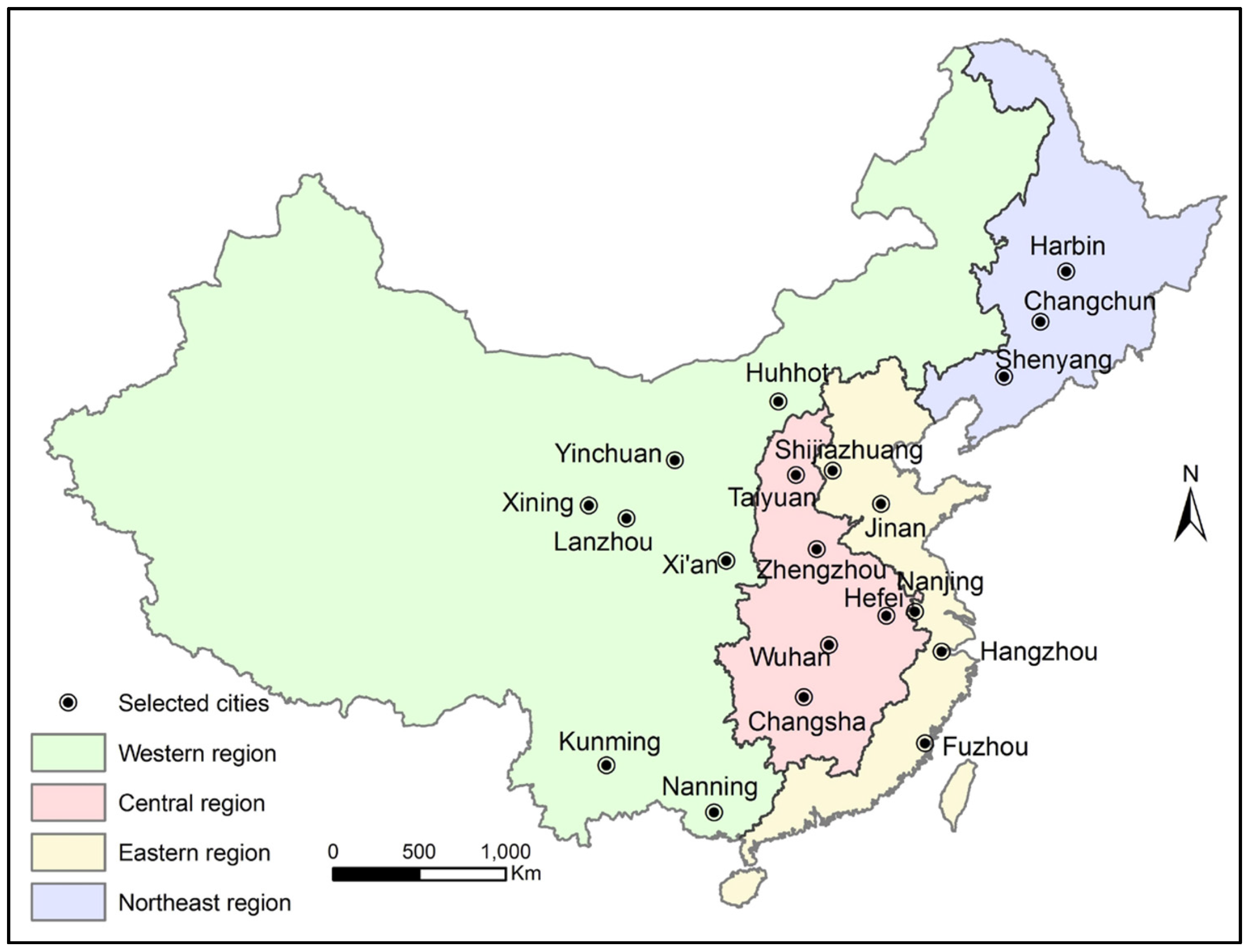
Figure 2.
NTL data for China obtained from Satellite F18 in 2010.

Figure 3.
The cumulative DN value of NTL data: (a) cumulative DN value without calibration; (b) cumulative DN value after intercalibration; (c) cumulative DN value after intra-annual correction; (d) cumulative DN value after inter-annual correction.
Figure 3.
The cumulative DN value of NTL data: (a) cumulative DN value without calibration; (b) cumulative DN value after intercalibration; (c) cumulative DN value after intra-annual correction; (d) cumulative DN value after inter-annual correction.
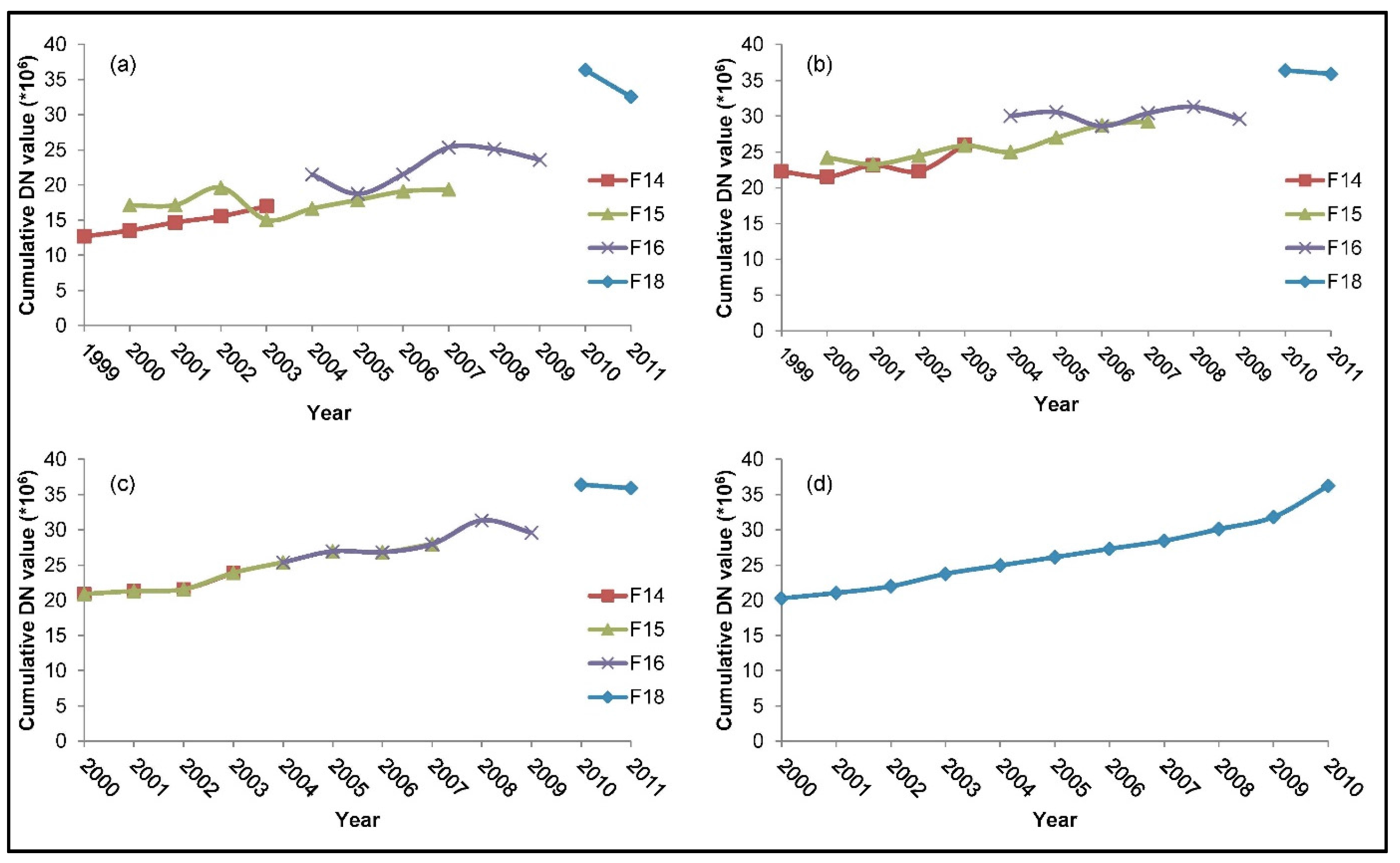
Figure 4.
R2 of three regression models (linear, exponential, power law) for energy consumption at province level.
Figure 4.
R2 of three regression models (linear, exponential, power law) for energy consumption at province level.

Figure 5.
Correlation analysis between the cumulative DN value of NTL data and statistical energy consumption for individual province.
Figure 5.
Correlation analysis between the cumulative DN value of NTL data and statistical energy consumption for individual province.

Figure 6.
The urban expansion of 20 cities in China during 2000–2010.
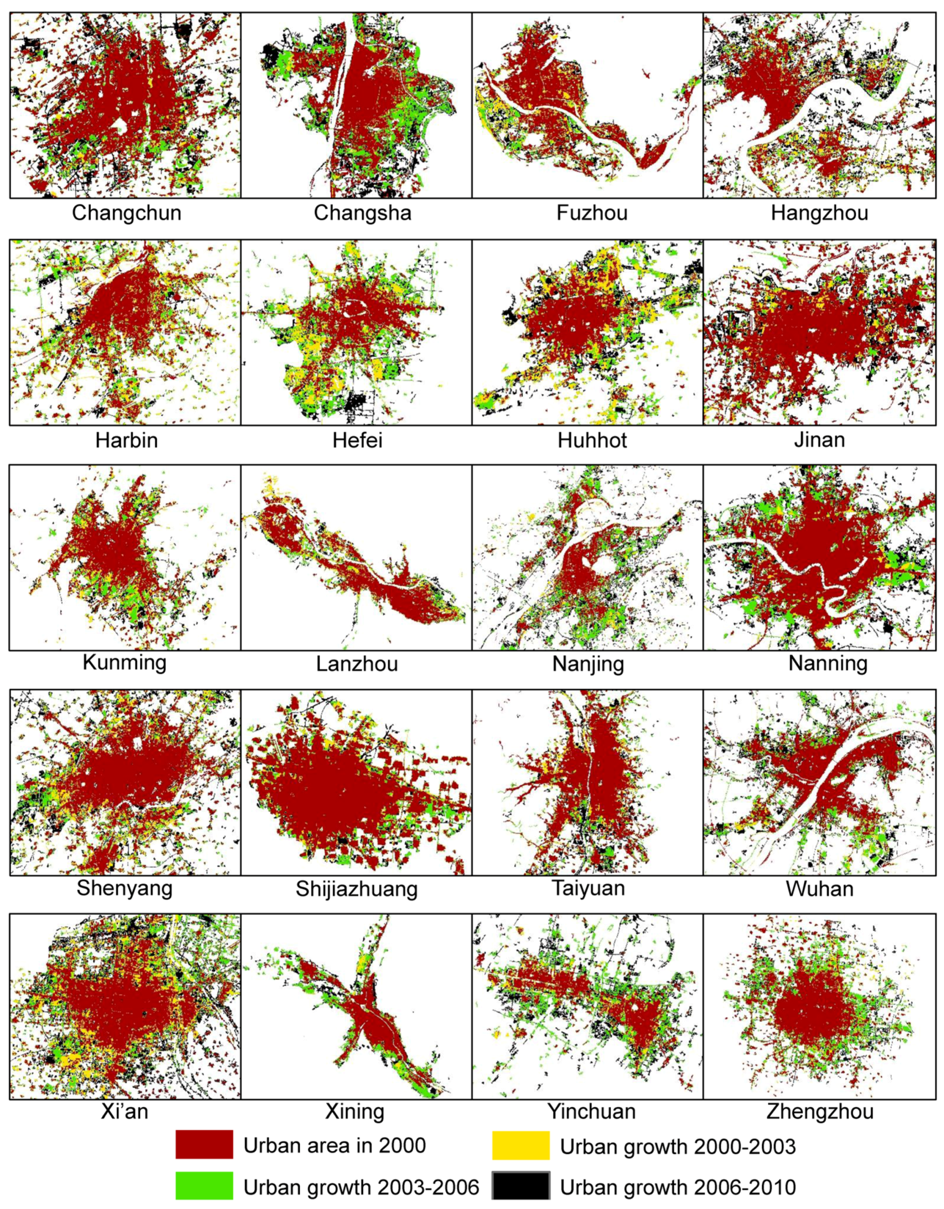
Figure 7.
Results of spatial metrics (FZ: Fuzhou; HZ: Hangzhou; JN: Jinan; NJ: Nanjing; SJZ: Shijiazhuang; CS: Changsha; HF: Hefei; TY: Taiyuan; WH: Wuhan; ZZ: Zhengzhou; HH: Huhhot; KM: Kunming; LZ: Lanzhou; NN: Nanning; XA: Xi’an; XN: Xining; YC: Yinchuan; CC: Changchun; HRB: Harbin; SY: Shenyang).

Figure 8.
The bar chart of energy consumptions for 20 cities from 2000 to 2010.


Table 1.
A list of 20 provincial capital cities.
| Capital City | Province |
|---|---|
| Changchun | Jilin |
| Changsha | Hunan |
| Fuzhou | Fujian |
| Hangzhou | Zhejiang |
| Harbin | Heilongjiang |
| Hefei | Anhui |
| Huhhot | Inner Mongolia |
| Jinan | Shandong |
| Kunming | Yunnan |
| Lanzhou | Gansu |
| Nanjing | Jiangsu |
| Nanning | Guangxi |
| Shenyang | Liaoning |
| Shijiazhuang | Hebei |
| Taiyuan | Shanxi |
| Wuhan | Hubei |
| Xi’an | Shaanxi |
| Xining | Qinghai |
| Yinchuan | Ningxia |
| Zhengzhou | Henan |
Table 2.
The parameters used to estimate energy consumption.
| Capital City | a | b | d2000 | d2003 | d2006 | d2010 |
|---|---|---|---|---|---|---|
| Changchun | 2.9496 × 10⁻⁵ | 1.4246 | 0.1234 | −0.0534 | −0.0208 | 0.1140 |
| Changsha | 2.2722 × 10⁻⁸ | 2.0431 | 0.0260 | 0.1201 | −0.1147 | 0.2345 |
| Fuzhou | 1.1910 × 10⁻⁷ | 1.839 | 0.0830 | −0.0172 | −0.0829 | 0.1215 |
| Hangzhou | 4.9712 × 10⁻⁷ | 1.6904 | −0.0491 | 0.0894 | −0.0339 | 0.0725 |
| Harbin | 1.2500 × 10⁻² | 0.9472 | −0.0167 | 0.0297 | −0.0731 | 0.0620 |
| Hefei | 2.3000 × 10⁻² | 0.9324 | 0.0052 | 0.0695 | −0.0369 | 0.0850 |
| Huhhot | 2.7631 × 10⁻⁶ | 1.6077 | 0.1653 | 0.0283 | −0.1528 | 0.3158 |
| Jinan | 1.2263 × 10⁻¹⁴ | 2.8376 | −0.0182 | −0.0272 | −0.0326 | 0.1499 |
| Kunming | 8.3172 × 10⁻⁵ | 1.3535 | 0.0210 | 0.0585 | −0.0979 | 0.1963 |
| Lanzhou | 1.9000 × 10⁻² | 0.961 | −0.0188 | 0.0235 | −0.1027 | 0.1427 |
| Nanjing | 7.8516 × 10⁻¹⁰ | 2.1024 | −0.0379 | 0.1720 | −0.0922 | 0.1438 |
| Nanning | 8.0950 × 10⁻⁶ | 1.5302 | 0.0244 | 0.0846 | −0.0981 | 0.1329 |
| Shenyang | 1.4536 × 10⁻⁷ | 1.8055 | −0.0146 | 0.0769 | −0.0336 | 0.1063 |
| Shijiazhuang | 1.4440 × 10⁻¹³ | 2.7024 | 0.0653 | −0.0472 | −0.1210 | 0.1820 |
| Taiyuan | 1.6499 × 10⁻¹⁰ | 2.2586 | 0.2244 | −0.0505 | −0.0963 | 0.2410 |
| Wuhan | 1.5720 × 10⁻⁷ | 1.8697 | 0.0531 | 0.0640 | −0.1142 | 0.2608 |
| Xi’an | 9.1232 × 10⁻⁶ | 1.4812 | 0.1615 | −0.0204 | −0.0482 | 0.1997 |
| Xining | 2.7388 × 10⁻⁴ | 1.3498 | −0.0605 | 0.1447 | −0.1101 | 0.1665 |
| Yinchuan | 7.3249 × 10⁻⁵ | 1.4174 | 0.1825 | −0.0658 | −0.0931 | 0.2610 |
| Zhengzhou | 2.2559 × 10⁻¹⁰ | 2.2131 | 0.0295 | 0.0170 | −0.0489 | 0.1349 |
Table 3.
Correlation coefficients of the selected spatial metrics.
| CA | NP | LPI | SHAPE_AM | ENN_AM | |
|---|---|---|---|---|---|
| CA | 1 | ||||
| NP | 0.795 ** | 1 | |||
| LPI | −0.098 | −0.376 ** | 1 | ||
| SHAPE_AM | 0.557 ** | 0.198 | 0.164 | 1 | |
| ENN_AM | 0.116 | 0.447 ** | −0.561 ** | −0.347 ** | 1 |
** Correlation is significant at the 0.01 level (2-tailed).
Table 4.
F-test results for models 1–4.
| F-Test | Model 1 | Model 2 | Model 3 | Model 4 |
|---|---|---|---|---|
| Pooled regression | 15.38 (F2) > F(57, 20) | 32.13 (F2) > F(57, 20) | 24.52 (F2) > F(57, 20) | 26.79 (F2) > F(57, 20) |
| (0.00001) | (0.00001) | (0.00001) | (0.00001) | |
| Variable intercepts and constant coefficients | 5.11 (F1) < F(38, 20) | 7.08 (F1) < F(38, 20) | 4. 99 (F1) < F(38, 20) | 4.07 (F1) < F(38, 20) |
| (0.00001) | (0.00001) | (0.00001) | (0.00001) |
Table 5.
Hausman test results for models.
| Model 1 | Model 2 | Model 3 | Model 4 | |||||
|---|---|---|---|---|---|---|---|---|
| Fixed | Random | Fixed | Random | Fixed | Random | Fixed | Random | |
| CA | 1.778 | 1.888 | 1.618 | 1.804 | ||||
| NP | 0.845 | 0.715 | ||||||
| LPI | 2.990 | −1.936 | −4.492 | −8.887 | ||||
| SHAPE_AM | 36.887 | 38.488 | 52.655 | 54.736 | ||||
| ENN_AM | −1.476 | −0.535 | ||||||
| W | 1.372 | 1.584 | 1.769 | 1.079 | ||||
Table 6.
Coefficients estimated from panel data analysis for 20 cities.
| Model 1 | Model 2 | Model 3 | Model 4 | |
|---|---|---|---|---|
| CA | 1.8423 ** | 1.5458 ** | ||
| t-statistic | 19.4988 | 10.5044 | ||
| NP | 0.9854 ** | |||
| t-statistic | 13.1153 | |||
| LPI | 3.4824 ** | −1.1637 | ||
| t-statistic | 2.9295 | −0.3902 | ||
| SHAPE_AM | 31.2928 ** | 49.4246 ** | ||
| t-statistic | 10.8085 | 15.8986 | ||
| ENN_AM | −2.1379 ** | |||
| t-statistic | −3.2791 | |||
| Constant | 112.9817 ** | 528.0465 ** | −458.4887 | −91.1109 * |
| t-statistic | 3.8604 | 3.9970 | −10.7452 | −2.3742 |
| Number of samples | 80 | 80 | 80 | 80 |
* Correlation is significant at the 0.05 level (2-tailed). ** Correlation is significant at the 0.01 level (2-tailed).
Table 7.
Coefficients estimated from panel data analysis for 5 cities in eastern region.
| Model 1 | Model 2 | Model 3 | Model 4 | |
|---|---|---|---|---|
| CA | 1.8419 ** | 0.5019 ** | ||
| t-statistic | 12.5977 | 3.2555 | ||
| NP | 0.9229 ** | |||
| t-statistic | 5.5859 | |||
| LPI | 3.5999 * | 11.2365 | ||
| t-statistic | 2.4055 | 1.3296 | ||
| SHAPE_AM | 41.8031 ** | 69.9353 ** | ||
| t-statistic | 4.7976 | 6.2613 | ||
| ENN_AM | −9.9416 ** | |||
| t-statistic | −7.6785 | |||
| Constant | 14.0176 | 1750.464 ** | −592.8746 ** | −593.4334 ** |
| t-statistic | 0.2683 | 8.3090 | −7.1441 | −3.4696 |
| Number of samples | 20 | 20 | 20 | 20 |
* Correlation is significant at the 0.05 level (2-tailed). ** Correlation is significant at the 0.01 level (2-tailed).
Table 8.
Coefficients estimated from panel data analysis for 5 cities in central region.
| Model 1 | Model 2 | Model 3 | Model 4 | |
|---|---|---|---|---|
| CA | 4.1585 ** | 2.7182 * | ||
| t-statistic | 5.5174 | 2.6012 | ||
| NP | 1.3567 ** | |||
| t-statistic | 7.6790 | |||
| LPI | −22.5420 ** | −8.3881 | ||
| t-statistic | −3.0637 | −1.0348 | ||
| SHAPE_AM | 36.1556 ** | 47.7420 ** | ||
| t-statistic | 8.8497 | 5.2764 | ||
| ENN_AM | 1.2017 | |||
| t-statistic | 0.2379 | |||
| Constant | −101.4677 | −100.0705 | −702.0447 ** | 38.0871 |
| t-statistic | −0.6874 | −0.1193 | −5.0798 | 0.3390 |
| Number of samples | 20 | 20 | 20 | 20 |
* Correlation is significant at the 0.05 level (2-tailed). ** Correlation is significant at the 0.01 level (2-tailed).
Table 9.
Coefficients estimated from panel data analysis for 7 cities in western region.
| Model 1 | Model 2 | Model 3 | Model 4 | |
|---|---|---|---|---|
| CA | 1.0872 ** | 0.4990 ** | ||
| t-statistic | 5.0936 | 3.1419 | ||
| NP | 1.1830 ** | |||
| t-statistic | 6.6968 | |||
| LPI | 25.9779 * | 10.8051 | ||
| t-statistic | 2.2129 | 0.8242 | ||
| SHAPE_AM | 14.2506 ** | 28.5075 ** | ||
| t-statistic | 2.8738 | 6.5706 | ||
| ENN_AM | −3.5386 ** | |||
| t-statistic | −4.3267 | |||
| Constant | 136.6374 * | 886.1985 ** | −173.8587 ** | −2.5220 |
| t-statistic | 2.4498 | 6.2931 | −3.1627 | −0.0378 |
| Number of samples | 28 | 28 | 28 | 28 |
* Correlation is significant at the 0.05 level (2-tailed). ** Correlation is significant at the 0.01 level (2-tailed).
Table 10.
Coefficients estimated from panel data analysis for 3 cities in northeast region.
| Model 1 | Model 2 | Model 3 | Model 4 | |
|---|---|---|---|---|
| CA | 1.5370 * | 0.2243 | ||
| t-statistic | 3.0651 | 0.3434 | ||
| NP | −0.2980 | |||
| t-statistic | −0.5863 | |||
| LPI | 7.7880 | 144.1321 * | ||
| t-statistic | 0.1489 | 2.5967 | ||
| SHAPE_AM | −10.3860 | 0.7350 | ||
| t-statistic | −2.1444 | 0.1554 | ||
| ENN_AM | 49.2399 | |||
| t-statistic | 2.0731 | |||
| Constant | 285.6944 | 237.0680 | 3627.8850 | 323.2328 |
| t-statistic | 1.4698 | 1.4159 | 2.2951 | 0.2830 |
| Number of samples | 12 | 12 | 12 | 12 |
* Correlation is significant at the 0.05 level (2-tailed).
© 2017 by the authors. Licensee MDPI, Basel, Switzerland. This article is an open access article distributed under the terms and conditions of the Creative Commons Attribution (CC BY) license (http://creativecommons.org/licenses/by/4.0/).
Share and Cite
MDPI and ACS Style
Zhao, J.; Thinh, N.X.; Li, C. Investigation of the Impacts of Urban Land Use Patterns on Energy Consumption in China: A Case Study of 20 Provincial Capital Cities. Sustainability 2017, 9, 1383. https://doi.org/10.3390/su9081383
AMA Style
Zhao J, Thinh NX, Li C. Investigation of the Impacts of Urban Land Use Patterns on Energy Consumption in China: A Case Study of 20 Provincial Capital Cities. Sustainability. 2017; 9(8):1383. https://doi.org/10.3390/su9081383
Chicago/Turabian StyleZhao, Jie, Nguyen Xuan Thinh, and Cheng Li. 2017. "Investigation of the Impacts of Urban Land Use Patterns on Energy Consumption in China: A Case Study of 20 Provincial Capital Cities" Sustainability 9, no. 8: 1383. https://doi.org/10.3390/su9081383
Note that from the first issue of 2016, this journal uses article numbers instead of page numbers. See further details here.