Analyzing the Impact of Nuclear Power on CO2 Emissions

1
Korea Energy Economics Institute, Ulsan 44543, Korea
2
Division of Economics, Pukyong National University, Busan 48513, Korea
*
Author to whom correspondence should be addressed.
Sustainability 2017, 9(8), 1428; https://doi.org/10.3390/su9081428
Submission received: 1 July 2017
/
Revised: 8 August 2017
/
Accepted: 10 August 2017
/
Published: 12 August 2017
(This article belongs to the Section Energy Sustainability)
Abstract
:This study investigates the relationship between the nuclear power proportion and CO2 emissions per capita using the panel dynamic ordinary least square method. The panel datasets consist of 18 countries covering 95% of the global nuclear reactors. The results indicate that a long-term 1% increase in nuclear power led to a 0.26–0.32% decrease in CO2 emissions per capita. Additionally, in France, Germany, and Switzerland they demonstrate the existence of the environmental Kuznets curve—an inverted U-shaped relationship between environmental pollution and income per capita.
1. Introduction
Nuclear power is an important means of reducing greenhouse gas emissions. The International Energy Agency (IEA) [1] proposes reduction measures such as demand management, energy efficiency improvement, carbon capture and storage, new and renewable energy, and nuclear power to hold the increase in global temperature below 2 °C above the pre-industrial level. It predicts that nuclear power use will increase to account for 15% of all annual greenhouse gas reductions by 2050. The Intergovernmental Panel on Climate Change [2] also highlights the benefit of nuclear power over other energy sources in terms of greenhouse gas emissions. It estimates the CO2 emissions coefficient for nuclear power over its life cycle as 12 tCO2/GWh, which represents a 40-fold reduction from the emissions coefficient of liquefied natural gas at 490 tCO2/GWh and a 68-fold reduction over that of coal at 820 tCO2/GWh. The International Atomic Energy Agency (IAEA) [3] emphasizes the role of nuclear power in achieving sustainable development and mitigating CO2 emissions in developing countries. IAEA [4] further presents the contribution of nuclear power to CO2 mitigation by showing that over the period 1970–2013, hydropower avoided 87 Gt CO2, nuclear power avoided 66 Gt CO2, and other renewables avoided 10 Gt CO2, respectively.
Recently, several studies attempted to investigate the relationship between nuclear power and CO2 emissions in the context of the environmental Kuznets curve (EKC) framework [5,6,7]. The original EKC hypothesis presumes an inverse U-shaped relationship between environmental pollution and income per capita (we refer readers to Kaika and Zervas [8] for an extensive overview of this topic). According to this hypothesis, the deterioration of the environment increases with income per capita during the initial stages of economic growth, but decreases with income per capita after arriving at a certain turning point. Research shows that the EKC hypothesis is explained through three channels: scale effect, composition effect, and technique effect [9]. Holding other effects constant, the scale effect is that emissions tend to rise proportionally as the scale of economic activity increases; the composition effect is that emissions can fall if an economy transits toward producing a set of goods that are cleaner and less polluting; the technique effect is that emissions can fall as cleaner techniques substitute for dirtier ones in the production of goods. Understandably, the EKC hypothesis can be accounted for with some mixture of scale, composition, and technique effects. The empirical evidence for this hypothesis is mixed at best, according to the estimation method, the data time periods and types, and the characteristics of countries [10].
There are mainly three research groups to examine the relationship between economic growth and environmental quality (we refer the reader to References [8,11,12,13,14] for a comprehensive survey). The first group investigates the relationship between economic development and environmental degradation in the framework of the EKC hypothesis. Recent studies include References [11,15,16,17]. The second group examines the relationship between economic development and energy consumption and tests the causal relationship between these variables. Payne [18] delivers an extensive review on this issue. The third group combines the two research groups by investigating the relationship among environmental degradation, economic growth, and energy consumption. Many recent studies focus on the impact of renewable energy on CO2 emissions in the EKC framework [12,13,19,20,21,22,23].
Consistent with the third research group focusing on nuclear power, Iwata et al. [5] estimated the EKC with the additional variable of nuclear power, and provided statistical evidence of the important role of nuclear power in reducing CO2 emissions. Similarly, Iwata et al. [6] investigated the EKC for CO2 emissions in 11 OECD countries by considering the role of nuclear power. These studies employ the autoregressive distributed lag (ARDL) model by Pesaran et al. [24] to consider the co-integration relation among their set of variables and analyze the role of nuclear power in reducing CO2 emissions on an individual country basis. The ARDL has econometric advantages, in that it can be used with a mixture of I(0) and I(1) variables, and estimate the short-run and long-run parameters simultaneously (a time-series is said to be I(d) variable if its d’th difference is stationary), as a single co-integration approach. Iwata et al. [7] also analyzed the impacts of nuclear energy on CO2 emissions using the pooled mean group (PMG) estimation method by Pesaran et al. [25]. Regarding nonstationary heterogeneous panels, the PMG approach allows the short-run coefficients to be heterogeneous but constrains the long-run coefficients to be identical across groups.
Although these studies convincingly argue the relationship between nuclear power and CO2 emissions, there are some limitations, in that the ARDL approach is based on individual countries and the PMG approach imposes that the long-run coefficient be homogenous across groups with nonstationary heterogeneous panels. To overcome such limitations, this study uses the panel dynamic ordinary least squares (PDOLS) method by Pedroni [26], which has the advantage of combining cross-sectional and time-series data to secure sufficient data points, and allows for the heterogeneity of coefficients across groups with nonstationary heterogeneous panels. This study aims to examine the relationship between the nuclear power proportion (the ratio of electricity produced from nuclear power to total electricity) and CO2 emissions per capita using the PDOLS method with nonstationary heterogeneous panels. The panel datasets in this study consist of 18 countries with more than four nuclear power plants each as of 2016, which operate 420 reactors, or approximately 95% of the 444 reactors worldwide. The results indicate that a long-term 1% increase in the nuclear power proportion leads to decreases of 0.26–0.32% in CO2 emissions per capita.
The main contribution of this study is, with the PDOLS approach, it provides statistical results as to how much nuclear power reduces CO2 emissions per capita for both the group mean and individual countries currently operating most of the nuclear reactors in the world. Additionally, this study compares nuclear power with renewable energy in terms of mitigating CO2 emissions.
2. Estimation Methodology
A three-stage procedure with nonstationary heterogeneous panels to analyze the relationship between the nuclear power proportion and CO2 emissions per capita is employed in this study. First, a panel unit root test suggested by Im, Pesaran, and Shin (IPS) [27] is conducted to check whether time-series variables in the datasets are stationary. Second, if the variables are not stationary, a panel co-integration test suggested by Pedroni [28] is used to assess whether the variables are characterized by a co-integration relation. Finally, if there is a co-integration relation among the variables, the econometric model in this study is estimated by using the PDOLS method.
2.1. Panel Unit Root Test
Prior to the PDOLS analysis, as a first step, the IPS test as a panel unit root test is conducted to check for the stationarity of time-series variables. Though the panel datasets in this study are unbalanced, the IPS test is known to be applicable for unbalanced panels. The following augmented Dickey–Fuller (ADF) regression model is estimated for the IPS test:
where (=1, 2, ..., N) is the number of cross-sectional data, (=1, 2, ..., T) is the number of time-series data, represents the first difference of each variable, is each variable under consideration in the econometric model, is the individual fixed effect, is the number of lags to remove serially correlated errors, and is the error term. The null hypothesis of the IPS test is that all panels contain a unit root ( for all ). The alternative hypothesis is that the fraction of panels is stationary ( for at least one ). The IPS test relaxes the assumption that all panels have a common autoregressive parameter . Instead, it allows for the heterogeneity of indexed by i. The IPS test conducts individual panel unit root tests for N number of cross-section units, and then the IPS t-bar statistic is based on the average value of individual ADF statistics as follows:
where is the value of the individual ADF statistic. IPS [27] shows that if the statistic is properly standardized, it is asymptotically standard normally distributed as follows:
2.2. Panel Co-Integration Test
Once each of the variables contains a panel unit root and is thus integrated of order one, I(1), as a second step, there needs to be a check for the relationship of co-integration among variables. Pedroni [28] proposes a method to check for a co-integration relationship among variables when multiple independent variables exist. The following regression model is estimated for Pedroni’s [28] panel co-integration test:
where (=1, 2, ..., N) is the number of cross-sectional data, (=1, 2, ..., T) is the number of time-series data, (=1, 2, ..., M) is the number of independent variables, is the dependent variable, is the independent variable, and is the error term. The individual fixed effect and the slope coefficient are permitted to vary across cross-sections. The estimated residuals from the above equation are structured as follows:
Regarding the estimated residuals as above, Pedroni [28] proposes seven test statistics to check for co-integration relationships in nonstationary panels. These seven statistics can be divided into two types. The first type is the “panel” statistics, including Panel v statistic, Panel rho statistic, Panel t statistic, Panel ADF statistic, based on pooling along the within-dimension. The second type is the “group-mean” statistics, including Group rho statistic, Group t statistic, Group ADF statistic, based on pooling the between-dimension. The seven test statistics are described in detail in Appendix A. The null hypothesis of no co-integration for both types is for all ; however, their alternative hypotheses are different. The alternative hypothesis for the “panel” statistics is for all , whereas the alternative hypothesis for the “group-mean” statistics is for all . Pedroni [28] derives asymptotic distribution and critical values for the seven test statistics via Monte Carlo simulation. The asymptotic distributions for each of the seven test statistics can be expressed as follows:
where is the properly standardized form for each of the seven test statistics, and and are the mean and variance adjustment terms, respectively. While Panel v statistic for a one-sided test diverges to positive infinity as the other test statistics diverge to negative infinity, the null hypothesis of no co-integration is rejected. Baltagi [29] states the intuition of rejection of the null hypothesis as follows: “Rejection of the null hypothesis means that enough of individual cross-sections have statistics ‘far away’ from the means predicted by theory were they to be generated under the null”.
2.3. Panel Dynamic Ordinary Least Squares
After determining the relationship of co-integration among variables, the econometric model can be estimated by using the PDOLS method developed by Pedroni [26]. The PDOLS estimator accounts for endogeneity in the regressors and serial correlation in the errors by including leads and lags of differenced endogenous variables as instruments. The PDOLS model in this study is as follows:
where is the emissions per capita, is the gross domestic product per capita, is the electricity production from nuclear power (the ratio of electricity produced from nuclear power to total electricity), and refer to leads and lags of differenced endogenous variables, and is the error term. Pedroni’s [26] PDOLS model allows for the heterogeneity of the coefficient between dimensions. This flexibility is an important advantage in the presence of heterogeneity of the co-integrating vectors. The group-mean PDOLS value indicates the average value of the individual coefficient between dimensions, and can be described as follows:
where indicates the DOLS of the individual .
2.4. The EKC Hypothesis for the Model
One representative variable that influences CO2 emissions is the GDP variable. The EKC hypothesis assumes increasing CO2 emissions during the early period of economic growth, followed by decreasing CO2 emissions when the economy is at a certain level of development. In other words, the EKC hypothesis assumes an inverted U-shaped relationship between the CO2 emissions and GDP. Validating the EKC hypothesis is a widely-studied topic, and represents a leading research area for the relationship between CO2 emissions and GDP. This study avoids the construction of an ad-hoc model in analyzing changes in CO2 emissions regarding changes in nuclear power proportion in this respect, but adds nuclear power proportion as an additional variable to the well-known EKC model. A similar attempt is utilized by Iwata et al. [5,6,7]. It is expected that has a positive value while has a negative one if the EKC hypothesis is valid for (7). Moreover, if there is an inverse relationship between nuclear power proportion and CO2 emissions per capita, it is expected that has a negative value.
3. Data
Countries with more than four operating nuclear reactors as of October 2016 were selected as the targets of this study. The total number of operable nuclear reactors worldwide is 444, with 100 reactors operated by the United States—the country most active in nuclear energy at the time of writing. The U.S. is followed by France, with 58 reactors, Japan, with 43 reactors, China, with 36 reactors, Russia, with 36 reactors, and Korea, with 25 reactors. Including these countries, the countries with more than four nuclear reactors in operation total 19. Slovakia currently operates four nuclear reactors, but is excluded from the analysis due to difficulties in accessing data. Table 1 provides an overview.
CO2 emissions per capita, GDP per capita, nuclear power proportion, and renewable energy proportion during 1970–2015 were collected from Enerdata [31] for each country. CO2 emissions are measured as metric ton per capita, GDP is measured in current U.S. dollars, nuclear power proportion is the ratio of electricity produced from nuclear power to total electricity, and renewable energy proportion is the ratio of electricity produced from renewable energy to total electricity. Renewable energies include hydro, wind, and solar energy.
Figure 1 shows the trends of CO2 emissions per capita for the 18 analyzed countries during the years from 1970 to 2015. The U.S. has the highest CO2 emissions per capita, followed by Canada, Korea, China, the Czech Republic, and Germany, in 2015. The trends in CO2 emissions per capita can be divided by countries experiencing an increase or decrease. The U.S. shows a decreasing trend, while Korea exhibits an increasing trend, for example.
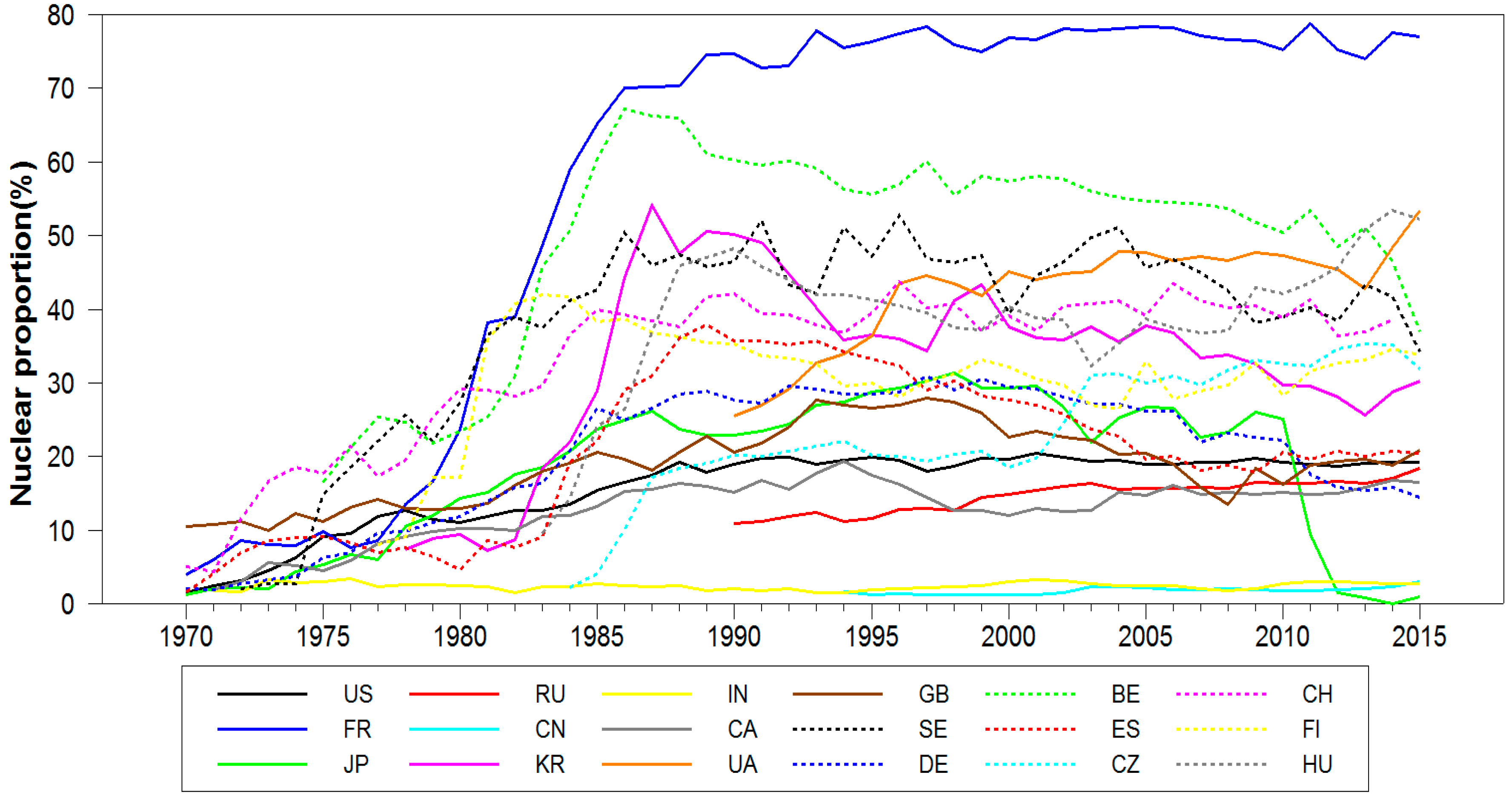
Figure 2 shows the nuclear power proportion of the 18 countries throughout 1970–2015. France has the highest nuclear power proportion, with more than 75% of its electricity generated by nuclear plants as of 2015, followed by Slovakia, Ukraine, Hungary, Switzerland, and Belgium. Regarding Japan, almost 25% of total electricity was produced from nuclear power in 2011 prior to the Fukushima nuclear power plant incident; however, the reactors have since ceased operating, with almost 0% of electricity from nuclear as of 2015.
4. Results
4.1. Estimation Results
Table 2 indicates the results of the IPS test, which is divided into two cases, where the time-series variable is level or the first difference. When the time-series variable is level, all variables were non-stationary, except for the nuclear power proportion variable in the case of the first difference; however, all variables were found to be stationary. Therefore, the panel unit root test indicates that each variable is integrated of order one, I(1), except for the nuclear power proportion variable.
Table 3 shows the results of the panel co-integration test proposed by Pedroni [28]. While the panel statistic nears positive infinity, or as the other statistics approach negative infinity, the null hypothesis of no co-integration relationship is rejected [29]. Table 3 shows there is a statistically significant co-integration relationship among CO2 emissions, GDP, and renewable energy proportion.
Given the presence of a co-integration relationship among the variables, the PDOLS model for nonstationary heterogeneous panels was estimated to analyze changes in CO2 emissions regarding changes in nuclear power proportions. Table 4 shows the results of the PDOLS estimates. The group-mean PDOLS estimates indicate that all coefficients are statistically significant. The results for the validation of the EKC hypothesis indicate that the hypothesis is valid within the analysis period, with values of = 0.3133, and = −0.02769. Considering that most countries operating nuclear reactors are advanced countries, these results are to be expected. was found to be −0.3233, indicating an inverse relationship between the nuclear power proportion and CO2 emissions per capita. This indicates that a long-term increase of 1% in the nuclear power proportion leads to a 0.32% decrease in CO2 emissions per capita during the analysis period.
PDOLS analysis also shows the DOLS values for individual countries. First, the countries with conditions that validated the EKC hypothesis were France, Russia, India, Sweden, Germany, and Switzerland. Second, countries with inverse relationships between nuclear power proportion and CO2 emissions per capita were the U.S., France, Japan, China, Korea, Canada, Ukraine, the United Kingdom, Germany, and Switzerland. Finally, the only three countries of the 18 analyzed meeting both conditions of valid EKC hypothesis and inverse relationships between nuclear power proportion and CO2 emissions per capita were France, Germany, and Switzerland.
Besides the nuclear power proportion variable, the PDOLS analysis was carried out, including a renewable energy proportion variable. Table 5 summarizes the analysis results. There were no meaningful differences between the analysis results shown in Table 4 in terms of the group-mean PDOLS estimates. All coefficients were found to be statistically significant, with = 0.3289 and = −0.05561, thus satisfying the EKC hypothesis. The nuclear power proportion, , is −0.2754, which is slightly lower than the previous results. The renewable energy proportion, , is −0.1092, which is lower than the coefficient for nuclear power proportion; however, as expected, an inverse relationship was found between the renewable energy proportion and CO2 emissions per capita.
When the analysis included the renewable energy proportion variable, there were no meaningful differences in the DOLS values for each country. Compared with the results in Table 4, countries with inverse relationships between nuclear power proportion and CO2 emissions per capita were the U.S., France, China, Canada, Ukraine, the United Kingdom, Germany, and Switzerland. These countries demonstrated robust results, but Japan and Korea are excluded from the results. When the analysis included the renewable energy proportion variable, the countries with both valid EKC hypothesis and inverse relationships between nuclear power proportion and CO2 emissions per capita were still the three previous countries of France, Germany, and Switzerland.
4.2. One Possible Implication
James Hansen is one of the first scientists to raise concerns about global climate change, and argues that 115 new reactors per year should be built by 2050 to avoid the worst effects of climate change [32]. His argument—which sounds rather extreme—is based on the claim that the 100% renewable scenarios are not realistic at all, and large amounts of nuclear power should close the energy gap. Here, we attempt to evaluate his argument based on the main findings of this study.
As of 2015, the average CO2 emissions per capita and nuclear power proportion for the 18 countries in this study are 5.93 metric tons and 14%, respectively [31]. Suppose that the reduction target for those countries is set to be a 20% cut in CO2 emissions per capita from 1990 levels and the target could be reached only by nuclear power. Then, the nuclear power proportion would need to extend from 14% to roughly 48–64% to achieve the target, based on the result that the estimated long-run elasticity of CO2 emissions per capita on nuclear power proportion is about 0.26–0.32%. Although the proportion to be raised is not an exact figure and cannot be directly comparable to Hansen’s suggestion, the main message is the same: nuclear power is the most urgent component of decarbonization—at least, in the near future.
5. Conclusions
This article investigates the impact of nuclear power generation on CO2 emissions by estimating the EKC with nuclear energy as an additional variable. The datasets encompass 18 countries with more than four nuclear reactors in operation during 1970–2015, thus covering approximately 95% of the number of nuclear reactors worldwide. PDOLS was employed as an estimation methodology to fully capture information from panel datasets.
The estimation results indicated that a long-term increase of 1% in the nuclear power proportion led to a 0.26–0.32% decrease in CO2 emissions per capita. Regarding individual countries, countries with robust inverse relationships between nuclear power proportion and CO2 emissions per capita were the U.S., France, China, Canada, Ukraine, the United Kingdom, Germany, and Switzerland. Additionally, countries with both valid EKC hypothesis and inverse relationships between nuclear power proportion and CO2 emissions per capita were France, Germany, and Switzerland. One possible implication of the estimation results is that the average nuclear power proportion for the 18 countries would need to extend from the 2015 level of 14% to approximately 48–64% to reduce CO2 emissions per capita by 20% below 1990 levels.
To conclude, the findings in this paper provide empirical evidence for the claim that nuclear power can contribute to reducing greenhouse gas emissions, while meeting the ever-increasing demand for energy. It is true that several OECD countries (e.g., France, Germany, recently South Korea, and Taiwan) have decided to lower the weight of nuclear power generation in their energy mix due to its potential catastrophic risks. However, nuclear power is still of importance to other countries—particularly developing ones—because it has a large, well-developed, and plentiful resource base as well as potentially favorable economics over other energy sources. The situation in each country is different; hence, the nuclear power option should be kept open under the Paris Agreement for parties that wish to include it and thereby enhance the cost effectiveness of their climate change mitigation actions.
Acknowledgments
This paper is partly based on the results from the Korean Economics Energy Institute Research Paper No. 2016-11.
Author Contributions
Sanglim Lee designed the research and wrote the paper; Minkyung Kim obtained the data and analyzed the results; and Jiwoong Lee improved and revised the manuscript. All authors provided comments on the manuscript and approved the final version.
Conflicts of Interest
The authors declare no conflict of interest.
Appendix A
The seven test statistics for a panel co-integration test are based on residual-based tests. Residuals , , and are collected from (4), (5), and the following regressions:
where (= 1, 2, ..., N) is the number of cross-sectional data, (= 1, 2, ..., T) is the number of time-series data, (= 1, 2, ..., M) is the number of independent variables, k (= 1, 2, …, K) is the number of lags. Next, with residuals , , and , the following terms are calculated:
Then, the seven test statistics are constructed with the appropriate terms described above. Details on how these statistics are constructed are discussed in Pedroni [28].
References
- IEA. Energy Technology Perspectives; OECD/IEA: Paris, France, 2015. [Google Scholar]
- Schlömer, S.; Bruckner, T.; Fulton, L.; Hertwich, E.; McKinnon, A.; Perczyk, D.; Roy, J.; Schaeffer, R.; Sims, R.; Smith, P.; et al. Annex III: Technology-specific cost and performance parameters. In Climate Change 2014: Mitigation of Climate Change; Contribution of Working Group III to the Fifth Assessment Report of the Intergovernmental Panel on Climate Change; Cambridge University Press: Cambridge, UK, 2014. [Google Scholar]
- IAEA. Nuclear Power for Greenhouse Gas Mitigation under the Kyoto Protocol: The Clean Development Mechanism (CDM); IAEA: Vienna, Austria, 2000. [Google Scholar]
- IAEA. Climate Change and Nuclear Power; IAEA: Vienna, Austria, 2016. [Google Scholar]
- Iwata, H.; Okada, K.; Samreth, S. Empirical study on the environmental Kuznets curve for CO2 in France: The role of nuclear energy. Energy Policy 2010, 38, 4057–4063. [Google Scholar] [CrossRef] [Green Version]
- Iwata, H.; Okada, K.; Samreth, S. A note on the environmental Kuznets curve for CO2: A pooled mean group approach. Appl. Energy 2011, 88, 1986–1996. [Google Scholar] [CrossRef]
- Iwata, H.; Okada, K.; Samreth, S. Empirical study on the determinants of CO2 emissions: Evidence from OECD countries. Appl. Econ. 2012, 44, 3513–3519. [Google Scholar] [CrossRef] [Green Version]
- Kaika, D.; Zervas, E. The Environmental Kuznets Curve (EKC) theory-Part A: Concept, causes and the CO2 emissions case. Energy Policy 2013, 62, 1392–1402. [Google Scholar] [CrossRef]
- Brock, W.A. Economic Growth and the Environment: A Review of Theory and Empirics. In Handbook of Economic Growth; Aghion, P., Durlauf, S.N., Eds.; Elsevier: Amsterdam, The Netherlands, 2005; Volume 1, pp. 1749–1821. [Google Scholar]
- Ajmi, A.N.; Hammoudeh, S.; Nyuyen, K.N.; Sato, J.R. A new look at the relationships between CO2 emissions, energy consumption and income in G7 countries: the importance of time variations. Energy Econ. 2015, 49, 629–638. [Google Scholar] [CrossRef]
- Ozturnk, I.; Al-Mulali, U. Investigating the validity of the environmental Kuznets curve hypothesis in Cambodia. Ecol. Indic. 2015, 57, 324–330. [Google Scholar] [CrossRef]
- Al-Mulali, U.; Saboori, B.; Ozturk, I. Investing the environmental Kuznets curve hypothesis in Vietnam. Energy Policy 2015, 76, 123–131. [Google Scholar] [CrossRef]
- Dogan, E.; Seker, F. The influence of real output, renewable and non-renewable energy, trade and financial development on carbon emissions in the top renewable energy countries. Renew. Sustain. Energy Rev. 2016, 60, 1074–1085. [Google Scholar] [CrossRef]
- Chen, P.Y.; Chen, S.T.; Hsu, C.S.; Chen, C.C. Modeling the global relationships among economic growth, energy consumption and CO2 emissions. Renew. Sustain. Energy Rev. 2016, 65, 420–431. [Google Scholar] [CrossRef]
- Apergis, N.; Ozturk, I. Testing Environmental Kuznet Curve hypothesis in Asian countries. Ecol. Indic. 2015, 52, 16–22. [Google Scholar] [CrossRef]
- Apergis, N. Environmental Kuznets curves: New evidence on both panel and country-level CO2 emissions. Energy Econ. 2016, 54, 263–271. [Google Scholar] [CrossRef]
- Apergis, N.; Christou, C.; Gupta, R. Are there Environmental Kuznets curves for US state-level CO2 emissions? Renew. Sustain. Energy Rev. 2017, 69, 551–558. [Google Scholar] [CrossRef]
- Payne, J.E. A survey of the electricity consumption-growth literature. Appl. Energy 2010, 87, 723–731. [Google Scholar] [CrossRef]
- Bölük, G.; Mert, M. Fossil & renewable energy consumption, GHGs (greenhouse gases) and economic growth: Evidence from a panel of EU (European Union) countries. Energy 2014, 74, 439–446. [Google Scholar] [CrossRef]
- Bölük, G.; Mert, M. The renewable energy, growth and environmental Kuznets curve in Turkey: An ARDL approach. Renew. Sustain. Energy Rev. 2015, 52, 587–595. [Google Scholar] [CrossRef]
- Al-mulali, U.; Tang, C.F.; Ozturk, I. Estimating the Environment Kuznets Curve hypothesis: Evidence from Latin America and the Caribbean countries. Renew. Sustain. Energy Rev. 2015, 50, 918–924. [Google Scholar] [CrossRef]
- Bilgili, F.; Koçak, E.; Bulut, Ü. The dynamic impact of renewable energy consumption on CO2 emissions: A revisited Environmental Kuznets Curve approach. Renew. Sustain. Energy Rev. 2016, 54, 838–845. [Google Scholar] [CrossRef]
- Jebli, M.B.; Yousserf, S.B.; Ozturk, I. Testing environmental Kuznets curve hypothesis: The role of renewable and non-renewable energy consumption and trade in OECD countries. Ecol. Indic. 2016, 60, 824–831. [Google Scholar] [CrossRef]
- Pesaran, M.H.; Shin, Y.; Smith, R.J. Bounds testing approaches to the analysis of level relationships. J. Appl. Econom. 2001, 16, 289–326. [Google Scholar] [CrossRef]
- Pesaran, M.H.; Shin, Y.; Smith, R.J. Pooled mean group estimation of dynamic heterogeneous panels. J. Am. Stat. Assoc. 1999, 94, 621–634. [Google Scholar] [CrossRef]
- Pedroni, P. Purchasing power parity tests in co-integrated panels. Rev. Econ. Stat. 2001, 83, 727–731. [Google Scholar] [CrossRef]
- Im, K.S.; Pesaran, M.H.; Shin, Y. Testing for unit roots in heterogeneous panels. J. Econom. 2003, 115, 53–74. [Google Scholar] [CrossRef]
- Pedroni, P. Critical values for co-integration tests in heterogeneous panels with multiple regressors. Oxf. Bull. Econ. Stat. 1999, 61, 653–670. [Google Scholar] [CrossRef]
- Baltagi, B.H. Econometric Analysis of Panel Data; John Wiley & Sons Ltd.: West Sussex, UK, 2005. [Google Scholar]
- IAEA PRIS. Available online: https://www.iaea.org/PRIS/ (accessed on 1 October 2016).
- Enerdata. Available online: http://www.enerdata.net (accessed on 1 October 2016).
- The Guardian. Available online: https://www.theguardian.com/environment/2015/dec/03/nuclear-power-paves-the-only-viable-path-forward-on-climate-change (accessed on 24 July 2017).
Figure 1.
Trends in CO2 emissions per capita. Top to bottom, left to right: U.S., France, Japan, Russia, China, Korea, India, Canada, Ukraine, United Kingdom, Sweden, Germany, Belgium, Spain, Czech Republic, Switzerland, Finland, and Hungary.
Figure 1.
Trends in CO2 emissions per capita. Top to bottom, left to right: U.S., France, Japan, Russia, China, Korea, India, Canada, Ukraine, United Kingdom, Sweden, Germany, Belgium, Spain, Czech Republic, Switzerland, Finland, and Hungary.
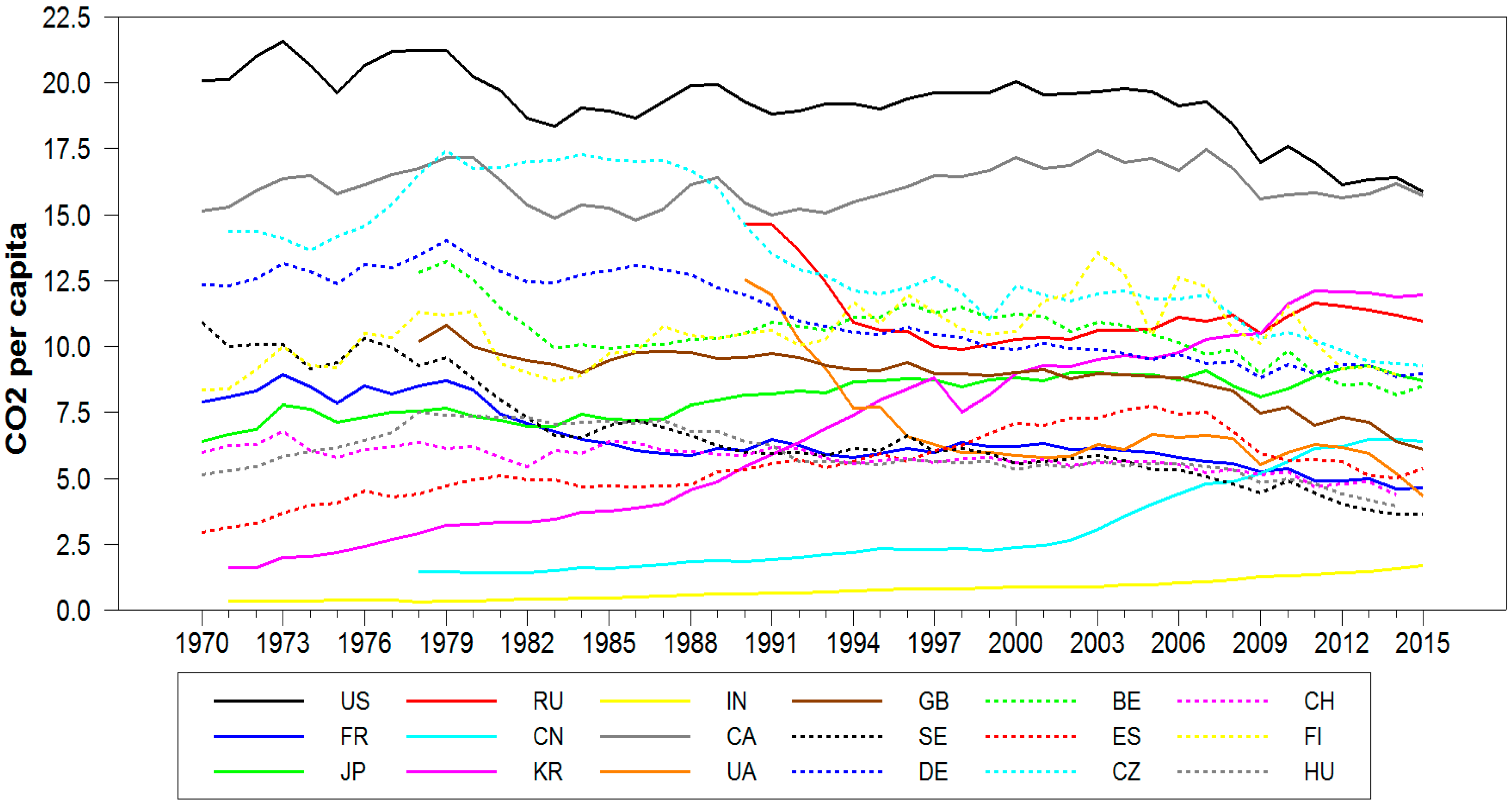
Figure 2.
Trends in nuclear power proportion. Top to bottom, left to right: U.S., France, Japan, Russia, China, Korea, India, Canada, Ukraine, United Kingdom, Sweden, Germany, Belgium, Spain, Czech Republic, Switzerland, Finland, and Hungary.
Figure 2.
Trends in nuclear power proportion. Top to bottom, left to right: U.S., France, Japan, Russia, China, Korea, India, Canada, Ukraine, United Kingdom, Sweden, Germany, Belgium, Spain, Czech Republic, Switzerland, Finland, and Hungary.


Table 1.
Nuclear power by country.
| Country | Number of Reactors | Total Net Electrical Capacity (MW) | |
|---|---|---|---|
| 1 | United States of America | 100 | 100,350 |
| 2 | France | 58 | 63,130 |
| 3 | Japan | 43 | 40,290 |
| 4 | China | 36 | 31,402 |
| 5 | Russia | 36 | 26,557 |
| 6 | Korea, Republic of | 25 | 23,133 |
| 7 | India | 22 | 6225 |
| 8 | Canada | 19 | 13,524 |
| 9 | Ukraine | 15 | 13,107 |
| 10 | United Kingdom | 15 | 8918 |
| 11 | Sweden | 10 | 9651 |
| 12 | Germany | 8 | 10,799 |
| 13 | Belgium | 7 | 5913 |
| 14 | Spain | 7 | 7121 |
| 15 | Czech Republic | 6 | 3930 |
| 16 | Switzerland | 5 | 3333 |
| 17 | Finland | 4 | 2752 |
| 18 | Hungary | 4 | 1889 |
| 19 | Slovakia | 4 | 1814 |
| 20 | Argentina | 3 | 1632 |
| 21 | Pakistan | 3 | 690 |
| 22 | Brazil | 2 | 1884 |
| 23 | Bulgaria | 2 | 1926 |
| 24 | Mexico | 2 | 1440 |
| 25 | Romania | 2 | 1300 |
| 26 | South Africa | 2 | 1860 |
| 27 | Armenia | 1 | 375 |
| 28 | Iran, Islamic Republic of | 1 | 915 |
| 29 | The Netherlands | 1 | 482 |
| 30 | Slovenia | 1 | 688 |
| Total | 444 | 387,030 |
Source: IAEA PRIS database [30].
Table 2.
Im, Pesaran, and Shin (IPS) panel unit root test.
| Variables | CO2 | GDP | GDP2 | Nuclear | Renewable |
|---|---|---|---|---|---|
| Level | −0.54 | 1.26 | −0.92 | −8.58 *** | −0.83 |
| First difference | −22.02 *** | −10.65 *** | −10.71 *** | - | −24.46 *** |
Note: * p < 0.1, ** p < 0.05, *** p < 0.01.
Table 3.
Pedroni panel co-integration test.
| Within-Dimension | Statistic Value | Between-Dimension | Statistic Value |
|---|---|---|---|
| Panel v | 5.202 *** | Group rho | –1.824 ** |
| Panel rho | –2.862 *** | Group t | –1.432 * |
| Panel t | –2.338 *** | Group ADF | –1.047 |
| Panel ADF | –1.443 * |
Note: * p < 0.1, ** p < 0.05, *** p < 0.01. ADF: augmented Dickey–Fuller statistic.
Table 4.
Panel dynamic ordinary least square results (case 1).
| Country | GDP | GDP2 | Nuclear | |
|---|---|---|---|---|
| 1 | United States | 0.0074 | −0.0384 | –0.7021 *** |
| (0.0379) | (−0.8028) | (–3.4290) | ||
| 2 | France | 0.3320 *** | −0.2786 *** | –0.2297 *** |
| (5.5760) | (−7.8350) | (–6.4320) | ||
| 3 | Japan | 0.0668 | −0.0090 | –0.1601 *** |
| (0.6562) | (−0.4563) | (–3.8270) | ||
| 4 | China | 0.4017 * | 0.1438 | –1.249 *** |
| (1.8630) | (1.3400) | (–8.4430) | ||
| 5 | Russia | 0.8055 *** | −0.0865 *** | 0.0972 *** |
| (10.7500) | (−7.5530) | (3.9850) | ||
| 6 | South Korea | 0.8770 *** | 0.3509 *** | –0.2305 ** |
| (2.8760) | (3.7230) | (–1.9780) | ||
| 7 | India | 0.3943 ** | −0.0910 *** | 0.4977 *** |
| (2.2160) | (−8.4410) | (4.2170) | ||
| 8 | Canada | 0.0277 | 0.0311 | –0.8216 *** |
| (0.1598) | (0.9807) | (–4.8630) | ||
| 9 | Ukraine | 0.4940 | −0.0371 | –1.6580 *** |
| (1.2040) | (−0.5274) | (–2.8900) | ||
| 10 | United Kingdom | 2.6510 *** | 0.2664 *** | –1.1380 ** |
| (2.9400) | (2.9160) | (–2.1810) | ||
| 11 | Sweden | 0.7005 *** | −0.3292 *** | –0.2848 |
| (4.9790) | (−6.3760) | (–1.6020) | ||
| 12 | Germany | 0.8374 *** | −0.2647 *** | –0.1167 *** |
| (10.8800) | (−13.0500) | (–2.5930) | ||
| 13 | Belgium | 0.0913 | −0.4068 *** | 0.4972 *** |
| (0.6179) | (−13.4800) | (7.1700) | ||
| 14 | Spain | −0.6068 ** | 0.0227 | –0.0792 |
| (−2.2920) | (0.7229) | (–1.6170) | ||
| 15 | Czech Rep. | −0.9325 *** | 0.1904 *** | 0.0842 * |
| (−6.3890) | (2.7760) | (1.8070) | ||
| 16 | Switzerland | 0.1916 *** | −0.0876 *** | –0.5492 *** |
| (2.7430) | (−3.0610) | (–2.6440) | ||
| 17 | Finland | 0.1498 | −0.0945 *** | 0.0985 * |
| (1.4820) | (−6.1760) | (1.8680) | ||
| 18 | Hungary | −0.849 *** | 0.2195 *** | 0.1261 ** |
| (−9.6590) | (5.2350) | (2.0610) | ||
| Panel group Number of observations: 738 | 0.3133 *** | −0.0277 *** | −0.3233 *** | |
| (7.220) | (−11.8000) | (−5.0420) | ||
Note: * p < 0.1, ** p < 0.05, *** p < 0.01. The numbers in parentheses are t-statistics for the corresponding coefficient.
Table 5.
Panel dynamic ordinary least square results (case 2).
| Country | GDP | GDP2 | Nuclear | Renewable | |
|---|---|---|---|---|---|
| 1 | United States | 0.1374 | −0.0439 | −0.5633 ** | –0.2159 |
| (0.7001) | (−1.2800) | (−2.4970) | (–0.7575) | ||
| 2 | France | 0.1344 | −0.2961 *** | −0.1552 *** | 0.2985 ** |
| (1.3010) | (−8.2850) | (−3.2080) | (2.4720) | ||
| 3 | Japan | −0.1695 | −0.0355 ** | −0.0164 | 1.232 *** |
| (−1.3640) | (1.9730) | (−0.3140) | (4.5000) | ||
| 4 | China | 0.2935 | 0.1016 | −1.0350 *** | –0.4016 |
| (1.1630) | (1.4460) | (−3.5640) | (–1.1420) | ||
| 5 | Russia | 0.9246 *** | −0.0881 *** | 0.1964 *** | 1.095 *** |
| (12.5300) | (−11.5700) | (8.4440) | (3.8720) | ||
| 6 | South Korea | 0.3833 *** | 0.1336 *** | 0.0325 | –0.3395 *** |
| (3.7700) | (2.7170) | (0.6884) | (–5.4760) | ||
| 7 | India | 0.2612 * | −0.03074 | 0.2106 | –0.8379 * |
| (1.7600) | (−0.9795) | (1.4520) | (–1.8750) | ||
| 8 | Canada | −0.1077 | −0.0143 | −0.8615 *** | –0.2166 |
| (−0.7220) | (−0.5613) | (−7.1650) | (–1.0660) | ||
| 9 | Ukraine | 0.3214 *** | 0.1346 *** | −0.7200 *** | –0.7918 *** |
| (7.3180) | (15.9200) | (−9.3120) | (–41.6900) | ||
| 10 | United Kingdom | 3.6000 *** | −0.0663 | −1.6570 *** | 1.2550 ** |
| (2.6380) | (−0.2826) | (−3.6330) | (2.0920) | ||
| 11 | Sweden | 0.8628 *** | −0.2550 *** | −0.4103 ** | –0.0457 |
| (4.9340) | (−5.8330) | (−2.5380) | (–0.2195) | ||
| 12 | Germany | 0.4603 ** | −0.1633 *** | −0.1239 *** | –0.1716 ** |
| (2.2050) | (−4.1320) | (−2.8390) | (–2.0880) | ||
| 13 | Belgium | −0.6908 *** | −0.3821 *** | 0.8756 *** | –0.4876 *** |
| (−3.2320) | (−14.0700) | (12.8400) | (–4.7660) | ||
| 14 | Spain | −0.7699 *** | −0.0065 | −0.0929 ** | –0.1371 |
| (−3.1680) | (−0.2353) | (−2.4180) | (–0.5018) | ||
| 15 | Czech Rep. | 0.0857 | 0.0163 | 0.0606 *** | –1.393 *** |
| (0.9190) | (0.6271) | (4.0640) | (–12.5400) | ||
| 16 | Switzerland | 0.1523 *** | −0.0537 *** | −0.9340 *** | –0.1201 |
| (4.6470) | (−2.8960) | (−4.3080) | (–1.5850) | ||
| 17 | Finland | 0.442 *** | −0.1076 *** | 0.195 *** | –0.4011 *** |
| (3.6720) | (−8.0210) | (3.4850) | (–2.7870) | ||
| 18 | Hungary | −0.4002 *** | 0.1563 *** | 0.0414 | –0.2862 *** |
| (−4.5150) | (7.1780) | (1.1580) | (–8.0880) | ||
| Panel group Number of observations: 738 | 0.3289 *** | −0.0556 *** | −0.2754 ** | −0.1092 *** | |
| (8.1440) | (−7.5970) | (−2.2770) | (−16.8900) | ||
Note: * p < 0.1, ** p < 0.05, *** p < 0.01. The numbers in parentheses are t-statistics for the corresponding coefficient.
© 2017 by the authors. Licensee MDPI, Basel, Switzerland. This article is an open access article distributed under the terms and conditions of the Creative Commons Attribution (CC BY) license (http://creativecommons.org/licenses/by/4.0/).
Share and Cite
MDPI and ACS Style
Lee, S.; Kim, M.; Lee, J. Analyzing the Impact of Nuclear Power on CO2 Emissions. Sustainability 2017, 9, 1428. https://doi.org/10.3390/su9081428
AMA Style
Lee S, Kim M, Lee J. Analyzing the Impact of Nuclear Power on CO2 Emissions. Sustainability. 2017; 9(8):1428. https://doi.org/10.3390/su9081428
Chicago/Turabian StyleLee, Sanglim, Minkyung Kim, and Jiwoong Lee. 2017. "Analyzing the Impact of Nuclear Power on CO2 Emissions" Sustainability 9, no. 8: 1428. https://doi.org/10.3390/su9081428
Note that from the first issue of 2016, this journal uses article numbers instead of page numbers. See further details here.