A Combined Voltage Control Strategy for Fuel Cell


1
Key Lab of Energy Thermal Conversion and Control of Ministry of Education, Southeast University, Nanjing 210096, China
2
School of Mechanical and Electrical Engineering, Qingdao University, Ningxia Road 308, Qingdao 266071, China
3
State Key Lab for Power Systems, Tsinghua University, Beijing 100084, China
4
Department of Electrical and Computer Engineering, Baylor University, Waco, TX 76798-7356, USA
*
Author to whom correspondence should be addressed.
Sustainability 2017, 9(9), 1517; https://doi.org/10.3390/su9091517
Submission received: 18 July 2017
/
Revised: 17 August 2017
/
Accepted: 22 August 2017
/
Published: 28 August 2017
(This article belongs to the Special Issue Sustainable Electric Power Systems Research)
Abstract
:Control of output voltage is critical for the power quality of solid oxide fuel cells (SOFCs), which is, however, challenging due to electrochemical nonlinearity, load disturbances, modelling uncertainties, and actuator constraints. Moreover, the fuel utilization rate should be limited within a safety range during the voltage regulation transient. The current research is usually appealing to model predictive control (MPC) by formulating the difficulties into a constrained optimization problem, but its huge computational complexity makes it formidable for real-time implementation in practice. To this end, this paper aims to develop a combined control structure, with basic function blocks, to fulfill the objectives with minor computation. Firstly, the disturbance, nonlinearity and uncertainties are lumped as a total disturbance, which is estimated and mitigated by active disturbance rejection controller (ADRC). Secondly, a feed-forward controller is introduced to improve the load disturbance rejection response. Finally, the constraints are satisfied by designing a cautious switching strategy. The simulation results show that the nominal performance of the proposed strategy is comparable to MPC. In the presence of parameter perturbation, the proposed strategy shows a better performance than MPC.
1. Introduction
Fuel cell electricity generation is considered to be the core of the future hydrogen industry [1]. Among the various types of fuel cells, solid oxide fuel cells (SOFCs) attract much attention for the purpose of large-scale power generation due to its high efficiency, long-term stability, fuel flexibility, low emissions, and avoiding the use of a precious platinum catalyst [2]. Moreover, it is able to internally reform the gas fuel to hydrogen for electrochemical reaction to generate electricity. From the control perspective, a significant advantage of the SOFC power plant is that its power can be adjusted conveniently, which is favorable for maintaining the stability of a microgrid.
Although theoretically promising, there still exist many practical issues that should be addressed for commercial applications. Efficient regulation of the SOFC output voltage during the load transient is one of the problems posed for controller design. The stability of the voltage is very important for the quality of the converted electricity. The control difficulties come from the system nonlinearity, rapid load disturbance and the constraints on the rate and amplitude of the manipulated actuator. Moreover, an aggressive control action may cause some potential risks in violating the safety range of the fuel utilization. Based on the benchmark model proposed in [3], it was revealed in [4,5] that the proportional-integral (PI) controller and even the H∞ optimal control are not able to give a satisfactory performance without exceeding the safety range of the fuel utilization.
To this end, the mainstream research resorts to Model Predictive Control (MPC), which is particularly suitable for constrained optimization. A data-driven linear MPC strategy was introduced in [6] based on the subspace identification. To further accommodate the nonlinearities, many nonlinear MPC (NMPC) strategyies [7,8,9,10] were developed based on much more complex heuristic models. The simulation results prove the capability of the above MPC methods under the nominal condition. However, the huge online computational requirement limits its wide application. Moreover, the implementation of MPC relies on a high-performance computer which needs to synchronously communicate with the existing Distributed Control System (DCS) through certain ports and protocols [11]. Additional hardware complexity will bring more security risks, which is not favored by the field engineers. Besides the complexity, another drawback of MPC is that the performance may deteriorate greatly in the presence of modelling uncertainties.
The industrial engineers argued in [12] that use of MPC is only suitable for the applications where the process size, complexity and potential economic benefits justify the expenditure and technical support requirements. In other words, it is not necessary to adopt MPC in the cases where the control objectives can also be fulfilled by the configuration of the regular function blocks, such as simple algebraic and logic computation components which can be easily accessed in the library of the mainstream devices. However, currently there is an obvious trend to indiscriminately formulate various problems in practice under a unified framework of constrained optimization and then simply transfer the computational burden to a high-performance computer, without any effort to attempt to use simple computation blocks along with the conventional approaches. Actually with the human’s intellectual effort and intuition, many control difficulties can be overcome by the combination of simple computation blocks. In this paper, the voltage control of the SOFC plant will be exemplified.
Up to now, proportional-integral-derivative (PID) controller still plays the dominant role in the whole industry. A recent survey [13] shows that the PID controller still accounts for more than 95% of the controllers utilized in the coal-fired power plant. However, PID controller is not sufficient in dealing with the processes in the presence of parametric perturbation. In the recent decade, active disturbance rejection control (ADRC) [14], which is inherited from PID control, is shown as a promising alternative to deal with nonlinearity and uncertainties, which are lumped as a ‘total disturbance’ that will be estimated and mitigated in real time. The efficiency has been validated by many practical applications in power control [15,16,17], process control [18,19] and by some theoretic analysis [20,21,22].
In our previous work, Ref. [23] deals with the advanced power conditioning control of SOFC system to improve the power quality. Ref. [24] is focused on the power coordination between SOFC power output and other renewables within a microgird. Ref. [25] attempts to improve the voltage regulation performance by introducing a feedforward scheme to the PI control system. The primary objective of this paper is to utilize ADRC to handle the nonlinearity and parametric uncertainties of the SOFC system.
Since the current load disturbance is measurable, a feedforward control structure is proposed to enhance the disturbance rejection ability. In light of the fuel utilization rate constraint, we propose a logical judgment block to complement the ability of ADRC. The basic idea is to switch the voltage control to fuel utilization control when the control system is approaching a dangerous condition.
The rest of the paper is organized as follows: the control difficulties of SOFC and the problems of MPC are analyzed in Section 2. Section 3 introduces the fundamentals of ADRC and its superiority in handling the nonlinearity over PID. The compound control structure and simulation results are presented in Section 4, and some conclusions are drawn in Section 5.
2. Problem Formulation
2.1. System Description
Nowadays, the highly-efficient SOFC power generation is considered as a promising candidate for stationary power generation. A significant feature that distinguishes SOFC from other fuel cells is the high operating temperature. It makes the SOFC suitable for combined heat and power generation which can further increase overall efficiency. Moreover, the high operating temperature makes it possible to internally reform the natural gas within the anode.
In this paper, the control research is based on a benchmark SOFC model [3], whose structure is shown in Figure 1. The controlled variable, manipulated variable and disturbance variable are the stack output voltage (V), natural gas flow rate (mol/s) and the external load current I (A), respectively. Some intermediate variables are the flow rates of the oxygen , the flow rates of the hydrogen and the partial pressures of hydrogen, oxygen, and steam, , and , respectively. The meanings and values of other parameters of the SOFC model are listed in Table 1.
Evidently, the block model in Figure 1 can be expressed as a nonlinear state-space model,
where the state variables are defined as representing the hydrogen mass flow and partial pressures of hydrogen, steam and oxygen. The output variable y is the output voltage . The input variable is the fuel flow rate , and the external disturbance denotes the load current, I. Note that the parameters are of nominal values, which may perturb during operation. In this paper, the perturbation, along with the plant characteristics perturbation, will be treated as total disturbance.
2.2. Control Difficulties
Generally, it is challenging to control a nonlinear plant by a linear control strategy because of the varying operating conditions. However, the control performance may deteriorate greatly if the process characteristics vary significantly with the operating conditions. To examine the nonlinearity of the SOFC plant, a common method is to compare the characteristics of the linearized models at different operating conditions [25,26]. Around the nominal operation point with = 0.7023 mol/s, I = 300 A, = 333 V, the nonlinear model (1) can be linearized as a transfer function model,
where
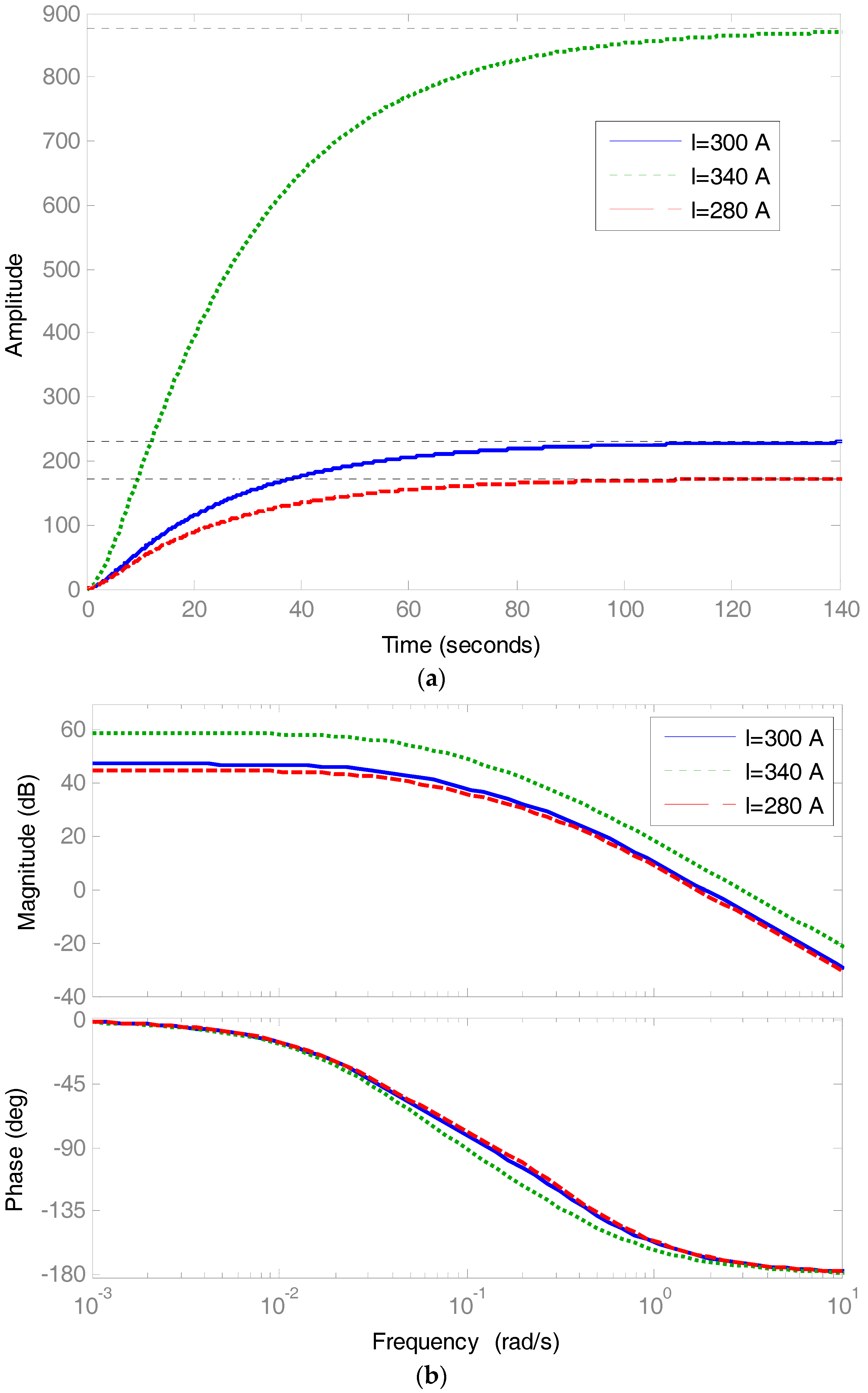
The nonlinearity of SOFC is exhibited via the step and frequency responses under the nominal condition as well as the varied conditions (I = 340 A and I = 280 A), as shown in Figure 2.
Obviously, the open-loop responses are quite sensitive to operating conditions, implying a strong nonlinearity of the SOFC system which should be taken into account for controller design. Besides the nonlinearity, another control difficulty for the SOFC plant is the hard constraint on the input magnitude and control change rate,
The most challenging difficulty is posed by the tight constraints on an operation variable, namely the fuel utilization factor defined by,
where, , and are the hydrogen input, output, and reacted flow rates, respectively.
Fuel utilization factor is a critical indicator for safety concern. A very big corresponds to an overspent fuel condition that can lead to fuel starvation and then damage the cells. A small implies that the feed fuel is underspent, which results in a low generation efficiency. Hence, both conditions should be avoided during operation. Generally, a reasonable operation range is recommended for fuel utilization as [10],
2.3. An Offset-Free MPC Solution
Most of the NMPC strategies are difficult to repeat and may cost huge computational burden. For illustrative purposes, this section adopts a widely-used industrial MPC which is based on the following discrete-time model,
where, the state variable , control input , measureable disturbance , and output variable are inherited from the continuous model (1). Note that a constant output disturbance is assumed and incorporated to augment the state variable, which can guarantee an offset-free steady state in spite of the presence of the uncertainties and unmeasurable disturbances. The matrices A, B, C, E and F can be obtained by linearizing the nonlinear model (1) under the nominal condition.
Generally, the optimization objective is
where is the current sampling instant, the set-point, the predicted output based on the model (8), and the control movement. The tuning parameters M, N and R corresponds to the control horizon, prediction horizon and the weighting parameter.
By setting the sampling time as 1 s, the fuel utilization constraint can be transformed to the input constraints based on the model. Combining (5)–(7), the restrictive conditions can be expressed as the final dynamic constraints [10],
Currently, the constrained receding horizon optimization problem (9)–(11) can be readily solved by quadratic programming (QP) method [27].
Although the above offset-free MPC solution can be realized through a standard routine, it suffers from a huge online computational burden which may harm the communication synchrony. Moreover, it risks the ill-conditioned matrix computation when the horizon parameters M and N are set larger than 10 [28]. What is worse, it is seen from the solution that both the optimal solution and the constraint satisfaction highly rely on the model accuracy. Once the model parameters perturb, the efficiency of MPC would have to deteriorate, which would be discussed in Section 5.
3. Combined Control Design
3.1. Fundamentals of ADRC
ADRC was theoretically developed based on a general n-th order description [14]. However, for the sake of simplicity, a second-order ADRC is widely used in practice with many successful results [29,30,31]. It has been theoretically justified in [32] that high-order processes can be controlled well by low-order ADRC. Figure 3 shows the basic control structure where is the reference and the process output, and and are controller parameters.
The root idea of ADRC is that, through an inner-loop compensation, an uncertain plant can be forced to behave like a canonical form, which can thus be simply controlled by an outer controller.
Firstly, the plant is organized as:
where is the gain parameter, the unknown dynamics, and the external disturbance. Denote as an estimation of the real value and . A total disturbance is defined as an extended state , then one can obtain
based on which, an extended state observer can be designed as
The observer states , , and are expected to track , , and , respectively. Although the dynamics of is neglected in (14), the convergence analysis of extended state observer (ESO) has been given in [33]. As shown in Figure 3, the ‘total disturbance’ is estimated and compensated,
which leads to a new equivalent plant from to ,
Evidently, the enhanced plant (16) can be approximated as cascaded integrators.
Secondly, based on the enhanced plant, the outer-loop control law can be designed as the proportional-derivative (PD) form,
where is a piecewise constant.
3.2. Parameter Tuning and Verification
Now there are mature methods available for ADRC tuning. Based on the bandwidth tuning [34],
where and correspond to explicit physical meanings, i.e., observer and closed-loop system bandwidths. Thus, the number of the tuning parameters can be reduced to three, i.e., and , all of which have explicit physical meanings [35].
To verify the compensation ability of ESO, the equivalent transfer function from to is derived precisely as
By rearranging the nominal model in (3) as , is tuned as 3.5509. The observer bandwidth is set as 4 rad/s to balance to the estimation accuracy and noise effects. Figure 4. shows the frequency responses of the equivalent transfer functions based on the linearized models around three operating points, as well as a model linearized around I = 300 A, but with approximately 30% perturbed model parameters, .
Compared with the open-loop frequency responses in Figure 2, it is seen that the behaviors of the compensated plants are quite similar to that of the ideal cascaded integrators in spite of the nonlinearity and parameter uncertainties, which is in accordance with our anticipation.
Based on the rule that ‘bigger bandwidth corresponds to a stronger observation and control ability, but a worse robustness’, the controller bandwidth is tuned as . A PID controller is tuned based on the nominal model (3) through a pole placement rule [36],
For comparison purposes, the desired pole of PID is determined to make the nominal performance between PID and ADRC similar. By neglecting all the constraints, the comparative simulation results between ADRC and PID are shown in Figure 5. Evidently, the performances of the ADRC and PID controller are similar under the nominal condition. However, the performances of the PID controller deteriorate significantly under the other operating conditions while the ADRC control system is almost immune to the condition variation. In this sense, it is again verified that ADRC has a strong ability to deal with parametric uncertainties, which is induced because of the system nonlinearity.
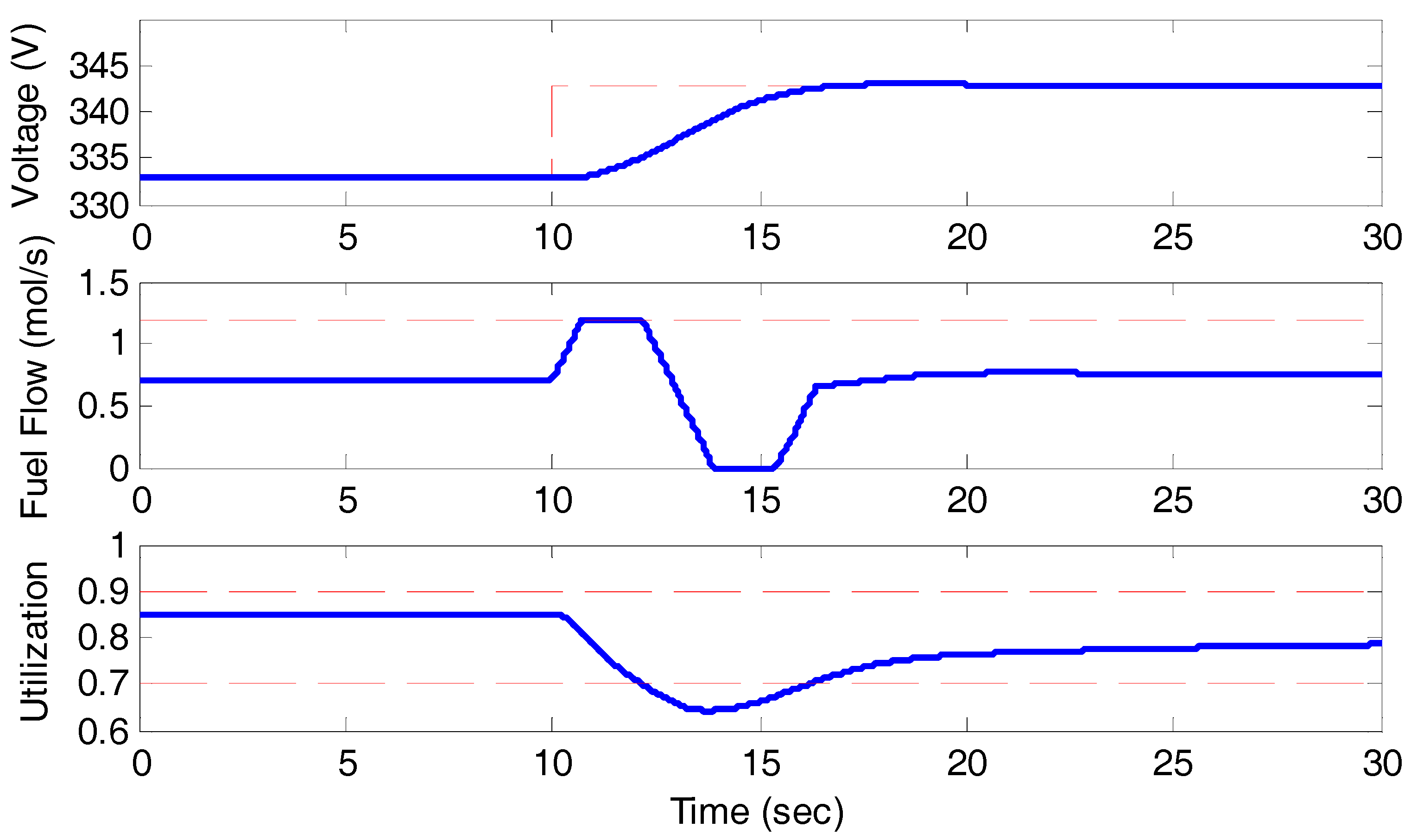
Finally, the performance of the ADRC control is further tested by incorporating the controller constraint (5). Figure 6 shows the simulation results, from which it can be seen that the fuel utilization factor exceeds the lower safety boundary 0.7 around 12~16 s. To this end, the next section will investigate a complementary strategy.
3.3. The Comprehensive Control Strategy
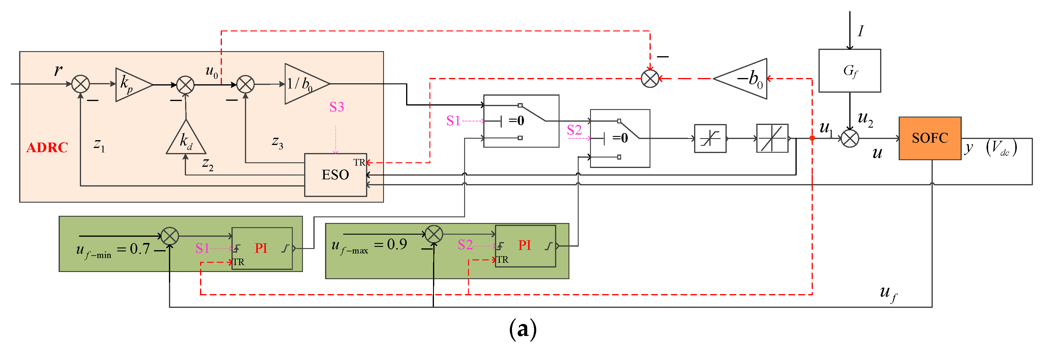
To avoid fuel utilization exceeding the safety range, a reasonable idea is to switch the voltage control (via ADRC) to fuel utilization control (via PI) when it tends to go over the border. Figure 7a shows the switching control structure, where the dash-dot pink line are logic signals (0 or 1) that determines the switching condition. The dashed red lines provides the initialization values for the controllers at the switching instant. Evidently, the switch will be activated from voltage control to fuel utilization regulation once S1 or S2 is set as 1. The logic signals are determined based on the process characteristics below,
- The rising command of the voltage requires the increment of the fuel feed, which would however decrease fuel utilization.
- The decreasing command of the voltage requires reducing the fuel feed, which would however increase fuel utilization.
Therefore, to avoid exceeding the lower boundary of fuel utilization, the logic signal S1 should be shifted to 1 (which means that voltage control is temporarily abandoned and the fuel utilization control is activated), once the following conditions are satisfied simultaneously: (i) the fuel utilization is below 0.7, and (ii) the output voltage is smaller than its set-point. If either of the conditions does not exist, S1 should be set as 0. The logic signal S2 can be designed based on similar thinking. The full triggering conditions are determined in Figure 7b.
3.4. Bumpless Transfer
With the switching objectives fulfilled, another practical problem is raised associated with the bumpless transfer. To guarantee a smooth switching from ADRC to PI, the integrators of the PI controller are set equal to the ADRC output, i.e., the Tracking Mode (TR) input to the PI controller, once there is a rising edge in the logic signal, S1 or S2.
Regardless of which control loop is activated, ESO always receive the real-time inputs and z1 and z2 can thus suitably track their corresponding values, respectively. Only z3 should be initialized as the “TR” input of ESO if there appears a falling edge in S3. The TR port of ESO can be readily determined by (15) and (17), with the aim to guarantee a bumpless transfer during the switch back to ADRC voltage control.
Since the fuel utilization control loop is of simple dynamics and only operates around a certain point (0.7 or 0.9), a PI controller is sufficient to regulate the fuel utilization staying at the boundaries,
Note that the in Figure 7a represents a feedforward compensation controller,
where is used to make the feedforward block proper.
4. Comparative Simulation
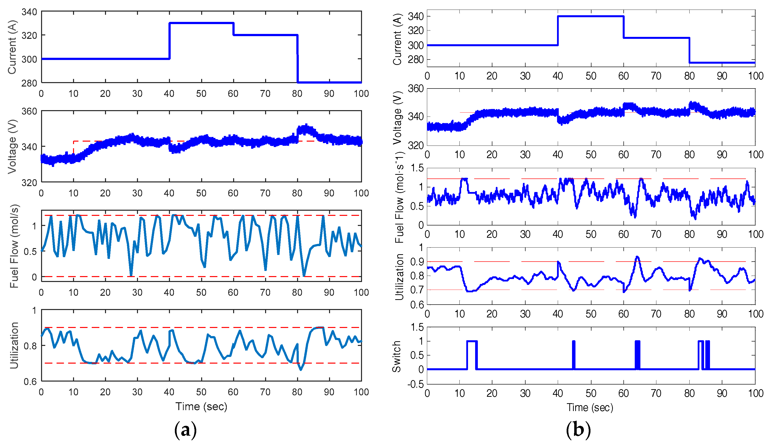
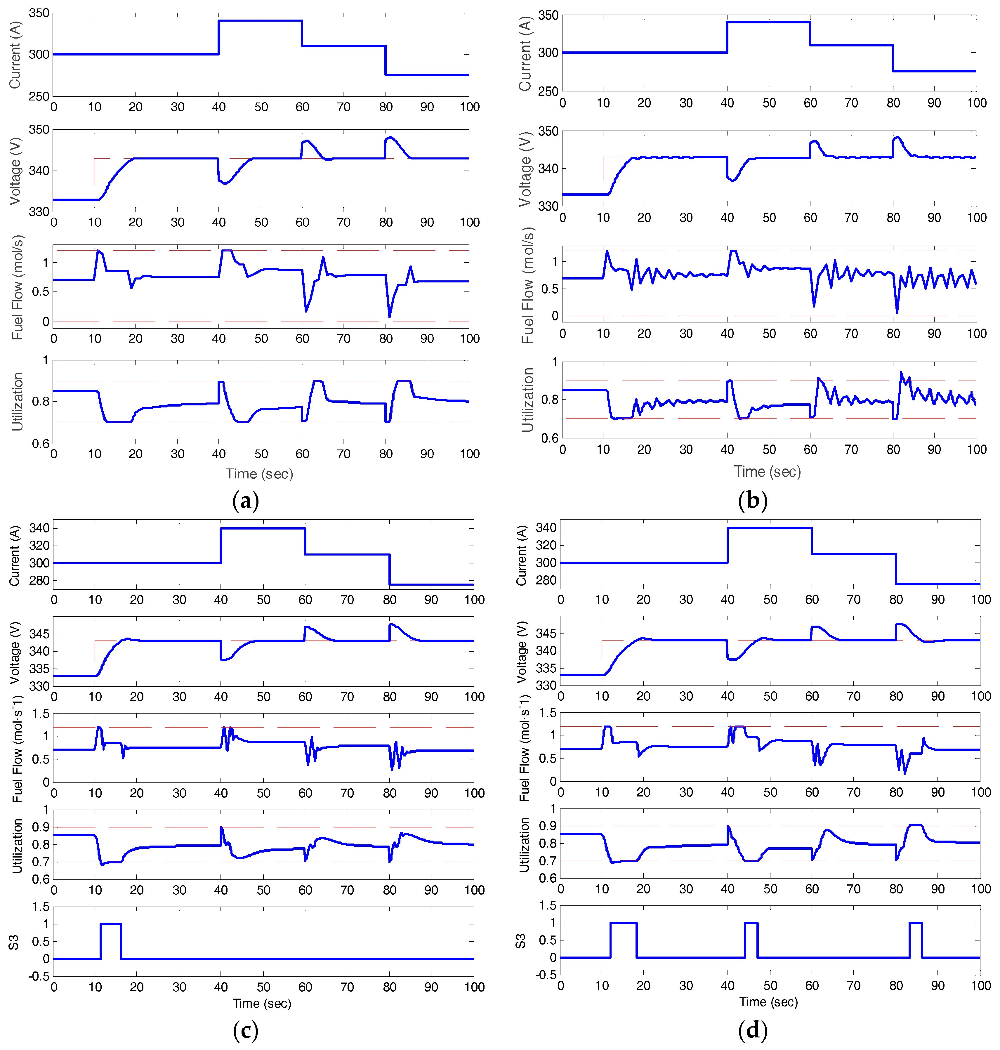
In this section, a simulation scenario, that will be tested based on the nonlinear model (1), is designed as follows: a step reference tracking command is added at t = 10 s and three load current disturbances are added at t = 40 s, 60 s, 80 s, respectively.
4.1. Simulation Results of MPC
On the basis of the problem formulated in Section 2.3, the parameters are tuned as: sampling period Ts = 1 s, the prediction horizon N = 10, control horizon M = 5 and the weighting factor R = 0.3. The simulation results based on the model (1) with accurate parameters in Table 1 are shown in Figure 8a. Obviously, the offset-free MPC produces a perfect set-point tracking and disturbance rejection while keeping the fuel utilization strictly within the safety boundary. Around t = 15 s, it can be found that the control input remains as constant when the fuel utilization is sliding along the safety border.
However, assuming the parameters are perturbed as following,, , , , the control performances are shown in Figure 8b. It can be seen that, with a model that deviates from its true plant characteristics, the control system exhibits deterioration. Moreover, the strict requirement on fuel utilization constraint cannot be satisfied at all. This problem will become more prominent with a worse model.
4.2. Simulation Results of the Proposed Control
With the proposed control structure shown in Section 3.3 and the parameters tuned in Section 3.2, the simulation results of the proposed control system based on the accurate nonlinear model are shown in Figure 8c. It can be found that the nominal performance is even comparable with that of MPC, although it took much less computation. The switching signal S3 shows the efficiency of the switching logic and bumpless transfer, guaranteeing the satisfaction of the fuel utilization constraint. When S3 is shifted to 1, the relay baton is transferred to fuel utilization control, waiting the output voltage slides to its reference.
Likewise, the simulation results of the proposed control system based on the model with perturbed parameters are shown in Figure 8d. Evidently, the control performances do not degrade too much, demonstrating the stronger robustness than that of MPC.
Another comparison is carried out by adding the sensor noise to the output voltage and increasing the time constants as , , , . The simulation results are shown in Figure 9. It shows that both control methods can handle sensor noise well but the proposed control structure demonstrates a less oscillatory fuel utilization rate.
Compared with the MPC solution, the proposed strategy features that (i) the control system can be configured using the basic computational components, where matrix inversion, numerical optimization and ill conditions are not involved; (ii) the controller design does not require an accurate model and thus insensitive to the modelling uncertainties.
4.3. Discussion
The MPC and ADRC exhibit different advantages in different aspects. Under the nominal condition, MPC achieves the best control performances with the least control effort. The proposed control strategy can also achieve a reasonable control performance. In the cases where the fuel utilization control is activated, a small output overshoot is present, which is inevitable due to the switching transient from PI to ADRC.
Under the perturbed condition, the performances of MPC degrade significantly, confirming that the regular MPC approach is sensitive to modeling uncertainties. However, in comparison, the proposed strategy in this paper produces a much more robust performance.
In summary, the proposed strategy shows obvious superiority over MPC in terms of computation intensity and realization complexity. All the ADRC, PI and logic blocks can be simply configured using regular components in the common industrial controllers.
5. Conclusions
Motivated by the computation complexity of MPC and its insufficiency in dealing with the parameter uncertainties, this paper investigates a practical control strategy for the voltage regulation of SOFCs. The nonlinearity of the plant is handled by ADRC. The constraint on the fuel utilization is satisfied by a switching control structure. The resulting problem of bumpless transfer is solved by an elaborate design. Compared with the performances of MPC, the simulation results show that the nominal performances of the proposed strategy are comparable with MPC and the perturbed performances are much better. This paper attempts to address that it is possible to realize an efficient SOFC voltage control system with simple computation complexity provided enough concern is given to the control design. The proposed strategy, consisting of active disturbance rejection control and some regular logic components, is shown as a promising alternative in the future SOFC control practices.
Acknowledgments
This work was supported by the Natural Science Foundation of Jiangsu Province, China under Grant BK20170686, National Natural Science Foundation of China under Grant 51576041, National Key Technology R&D Program under Grant 2016YFB0901405, the Fundamental Research Funds for the Central Universities in China under grant 3203007452 and open fund from state key lab of power systems under grant SKLD17MK11. The authors would like to give our heartfelt thanks to anonymous reviewers for the careful review and penetrating suggestions in improving the paper.
Author Contributions
All authors collectively conceived the research and carried out the analysis. L.S., Q.H., and H.F. led the simulation and paper writing with contributions and guidance from J.S, Y.X., D.L. and K.Y.L.
Conflicts of Interest
The authors declare no conflicts of interest.
References
- Cruz Rojas, A.; Lopez Lopez, G.; Gomez-Aguilar, J.; Alvarado, V.; Sandoval Torres, C. Control of the Air Supply Subsystem in a PEMFC with Balance of Plant Simulation. Sustainability 2017, 9, 73. [Google Scholar] [CrossRef]
- Suther, T.; Fung, A.; Koksal, M.; Zabihian, F. Macro level modeling of a tubular solid oxide fuel cell. Sustainability 2010, 2, 3549–3560. [Google Scholar] [CrossRef]
- Padulles, J.; Ault, G.W.; McDonald, J.R. An integrated SOFC plant dynamic model for power systems simulation. J. Power Sources 2000, 86, 495–500. [Google Scholar] [CrossRef]
- Li, Y.H.; Choi, S.S.; Rajakaruna, S. An analysis of the control and operation of a solid oxide fuel-cell power plant in an isolated system. IEEE Trans. Energy Convers. 2005, 20, 381–387. [Google Scholar] [CrossRef]
- Knyazkin, V.; Söder, L.; Canizares, C. Control challenges of fuel cell-driven distributed generation. In Proceedings of the 2003 IEEE Bologna Power Tech Conference Proceedings, Bologna, Italy, 23–26 June 2003; Volume 2, p. 2. [Google Scholar]
- Wang, X.; Huang, B.; Chen, T. Data-driven predictive control for solid oxide fuel cells. J. Process Control 2007, 17, 103–114. [Google Scholar] [CrossRef]
- Zhang, X.W.; Chan, S.H.; Ho, H.K.; Li, J.; Li, G.; Feng, Z. Nonlinear model predictive control based on the moving horizon state estimation for the solid oxide fuel cell. Int. J. Hydrog. Energy 2008, 33, 2355–2366. [Google Scholar] [CrossRef]
- Huo, H.B.; Zhu, X.J.; Hu, W.Q.; Tu, H.-Y.; Li, J.; Yang, J. Nonlinear model predictive control of SOFC based on a Hammerstein model. J. Power Sources 2008, 185, 338–344. [Google Scholar] [CrossRef]
- Wu, X.J.; Zhu, X.J.; Cao, G.Y.; Tu, H.-Y. Predictive control of SOFC based on a GA-RBF neural network model. J. Power Sources 2008, 179, 232–239. [Google Scholar] [CrossRef]
- Li, Y.; Shen, J.; Lu, J. Constrained model predictive control of a solid oxide fuel cell based on genetic optimization. J. Power Sources 2011, 196, 5873–5880. [Google Scholar] [CrossRef]
- Wu, X.; Shen, J.; Li, Y.; Lee, K.Y. Hierarchical optimization of boiler-turbine unit using fuzzy stable model predictive control. Control Eng. Pract. 2014, 30, 112–123. [Google Scholar] [CrossRef]
- Wade, H.L. Inverted decoupling: A neglected technique. ISA Trans. 1997, 36, 3–10. [Google Scholar] [CrossRef]
- Sun, L.; Li, D.; Lee, K.Y. Optimal disturbance rejection for PI controller with constraints on relative delay margin. ISA Trans. 2016, 63, 103–111. [Google Scholar] [CrossRef] [PubMed]
- Han, J. From PID to active disturbance rejection control. IEEE Trans. Ind. Electron. 2009, 56, 900–906. [Google Scholar] [CrossRef]
- Li, D.; Li, C.; Gao, Z.; Jin, Q. On active disturbance rejection in temperature regulation of the proton exchange membrane fuel cells. J. Power Sources 2015, 283, 452–463. [Google Scholar] [CrossRef]
- Huang, C.E.; Li, D.H.; Xue, Y. Active disturbance rejection control for the ALSTOM gasifier benchmark problem. Control Eng. Pract. 2013, 21, 556–564. [Google Scholar] [CrossRef]
- Liang, G.; Li, W.; Li, Z. Control of superheated steam temperature in large-capacity generation units based on active disturbance rejection method and distributed control system. Control Eng. Pract. 2013, 21, 268–285. [Google Scholar] [CrossRef]
- Li, D.; Li, Z.; Gao, Z.; Jin, Q. Active disturbance rejection-based high-precision temperature control of a semibatch emulsion polymerization reactor. Ind. Eng. Chem. Res. 2014, 53, 3210–3221. [Google Scholar] [CrossRef]
- Sun, L.; Dong, J.; Li, D.; Lee, K.Y. A practical multivariable control approach based on inverted decoupling and decentralized active disturbance rejection controller. Ind. Eng. Chem. Res. 2016, 55, 2008–2019. [Google Scholar] [CrossRef]
- Zheng, Q.; Chen, Z.; Gao, Z. A practical approach to disturbance decoupling control. Control Eng. Pract. 2009, 17, 1016–1025. [Google Scholar] [CrossRef]
- Sun, L.; Li, D.H.; Gao, Z.; Yang, Z.; Zhao, S. Combined feedforward and model-assisted active disturbance rejection control for non-minimum phase system. ISA Trans. 2016, 64, 24–33. [Google Scholar] [CrossRef] [PubMed]
- Guo, B.Z.; Zhou, H.C. The active disturbance rejection control to stabilization for multi-dimensional wave equation with boundary control matched disturbance. IEEE Trans. Autom. Control 2015, 60, 143–157. [Google Scholar] [CrossRef]
- Wu, G.; Sun, L.; Lee, K.Y. Disturbance rejection control of a fuel cell power plant in a grid-connected system. Control Eng. Pract. 2017, 60, 183–192. [Google Scholar] [CrossRef]
- Sun, L.; Wu, G.; Xue, Y.; Shen, J.; Li, D.; Lee, K.Y. Coordinated Control Strategies for SOFC Power Plant in a Microgrid. IEEE Trans. Energy Convers. 2017. [Google Scholar] [CrossRef]
- Sun, L.; Li, D.; Wu, G.; Lee, K.Y.; Xue, Y. A Practical Compound Controller Design for Solid Oxide Fuel Cells. In Proceedings of the 9th IFAC Symposium on Control of Power and Energy Systems (CPES), Delhi, India, 9–11 December 2015; pp. 445–449. [Google Scholar]
- Sun, L.; Li, D.; Lee, K.Y. Enhanced decentralized PI control for fluidized bed combustor via advanced disturbance observer. Control Eng. Pract. 2015, 42, 128–139. [Google Scholar] [CrossRef]
- Schmid, C.; Biegler, L T. Quadratic programming methods for reduced hessian SQP. Comput. Chem. Eng. 1994, 18, 817–832. [Google Scholar] [CrossRef]
- Wang, L. Model predictive control: Design and implementation using MATLAB. In Proceedings of the 2009 American Control Conference, St. Louis, MO, USA, 10–12 June 2009; pp. 25–26. [Google Scholar]
- Li, M.; Li, D.; Wang, J.; Zhao, C. Active disturbance rejection control for fractional-order system. ISA Trans. 2013, 52, 365–374. [Google Scholar] [CrossRef] [PubMed]
- Sun, L.; Dong, J.; Li, D.H. Active disturbance rejection control for superheated steam boiler temperatures using the fruit fly algorithm. J. Tsinghua Univ. 2014, 54, 1288–1292. [Google Scholar]
- Zhang, Y.; Li, D.H.; Gao, Z.; Zheng, Q. On oscillation reduction in feedback control for processes with an uncertain dead time and internal-external disturbances. ISA Trans. 2015, 59, 29–38. [Google Scholar] [CrossRef] [PubMed]
- Zhao, C.; Li, D. Control design for the SISO system with the unknown order and the unknown relative degree. ISA Trans. 2014, 53, 858–872. [Google Scholar] [CrossRef] [PubMed]
- Zheng, Q.; Gao, L.; Gao, Z. On stability analysis of active disturbance rejection control for nonlinear time-varying plants with unknown dynamics. In Proceedings of the IEEE Conference on Decision and Control, New Orleans, LA, USA, 12–14 December 2007. [Google Scholar]
- Gao, Z. Scaling and bandwidth-parameterization based controller tuning. In Proceedings of the 2003 American Control Conference, 4–6 June 2003; Volume 6, pp. 4989–4996. [Google Scholar]
- Zhang, Y.; Li, D.; Xue, Y. Active disturbance rejection control for circulating fluidized bed boiler. In Proceedings of the 2012 12th International Conference on Control, Automation and Systems (ICCAS), JeJu Island, Korea, 17–21 October 2012; pp. 1413–1418. [Google Scholar]
- Åström, K.J.; Hägglund, T. Advanced PID Control; ISA—The Instrumentation, Systems, and Automation Society: Triangle Park, NC, USA, 2006. [Google Scholar]
Figure 1.
The benchmark solid oxide fuel cell (SOFC) model.
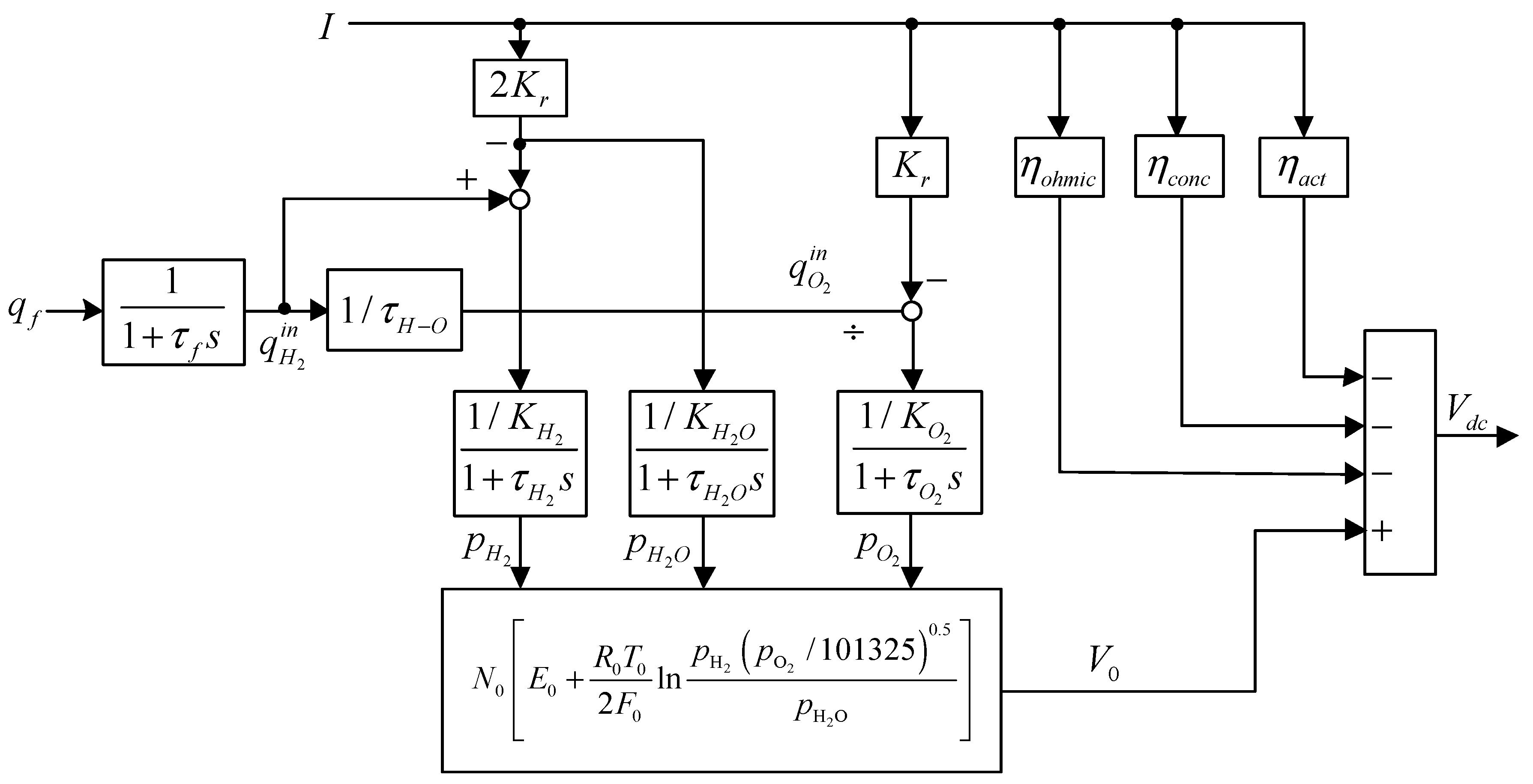
Figure 2.
The comparison of the step responses (a) and frequency responses (b) under different conditions.
Figure 2.
The comparison of the step responses (a) and frequency responses (b) under different conditions.

Figure 3.
The basic control structure of a second-order active disturbance rejection control (ADRC).
Figure 3.
The basic control structure of a second-order active disturbance rejection control (ADRC).
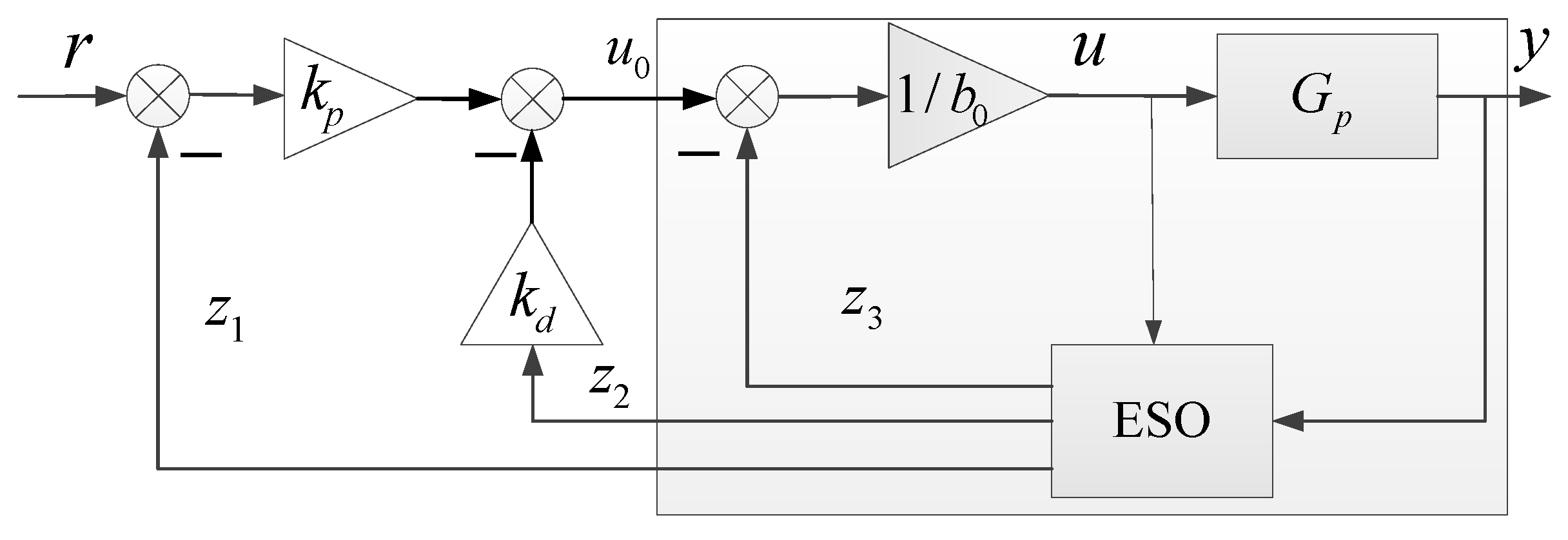
Figure 4.
Frequency responses of the pure cascaded integrators and various equivalent compensated plants.
Figure 4.
Frequency responses of the pure cascaded integrators and various equivalent compensated plants.
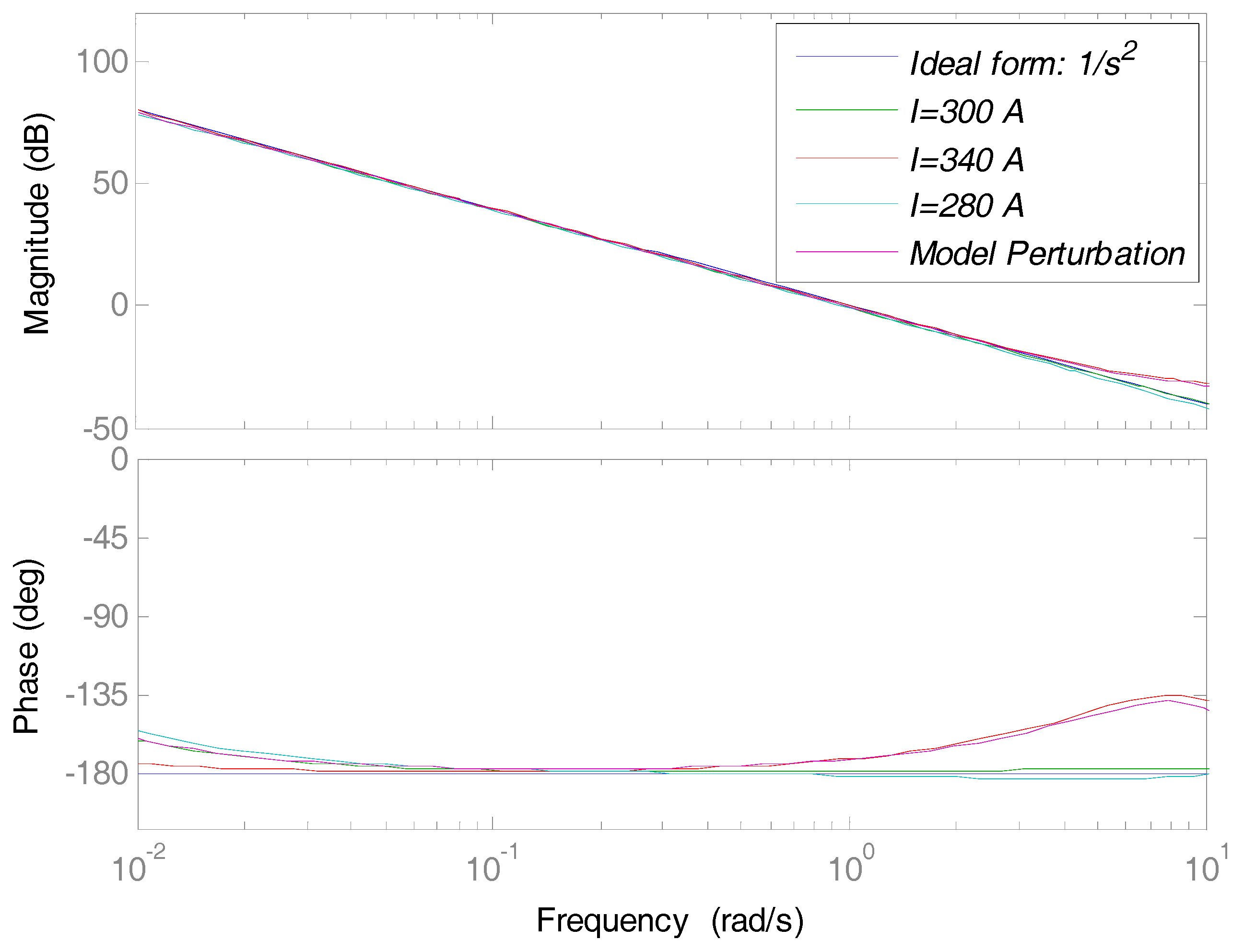
Figure 5.
Comparative results between ADRC and PID control without constraints taken into account.
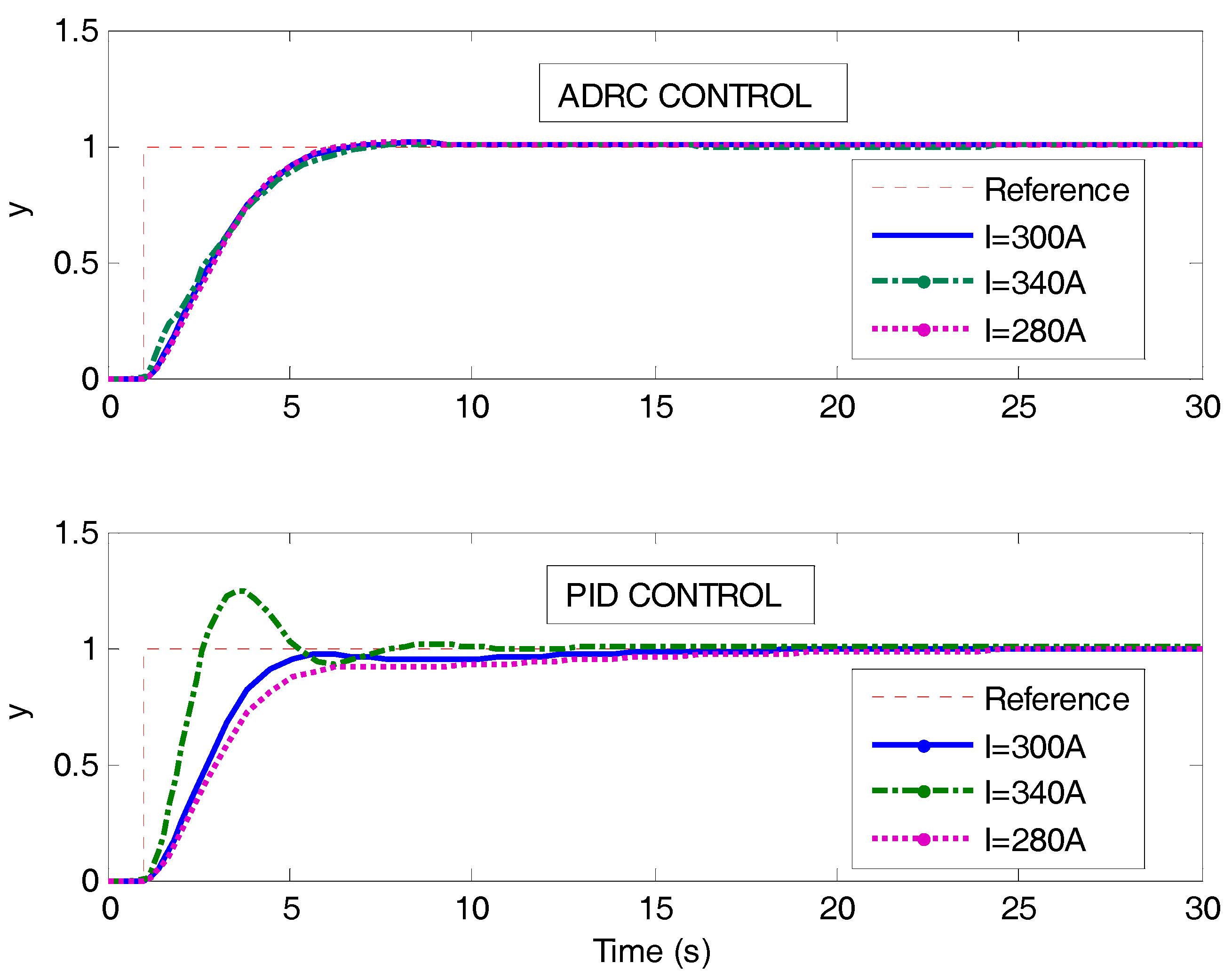
Figure 6.
The performances of the ADRC control system where the controller constraints are considered.
Figure 6.
The performances of the ADRC control system where the controller constraints are considered.

Figure 7.
The illustration of the switching control system. (a) Switching structure; (b) Triggering conditions.
Figure 7.
The illustration of the switching control system. (a) Switching structure; (b) Triggering conditions.

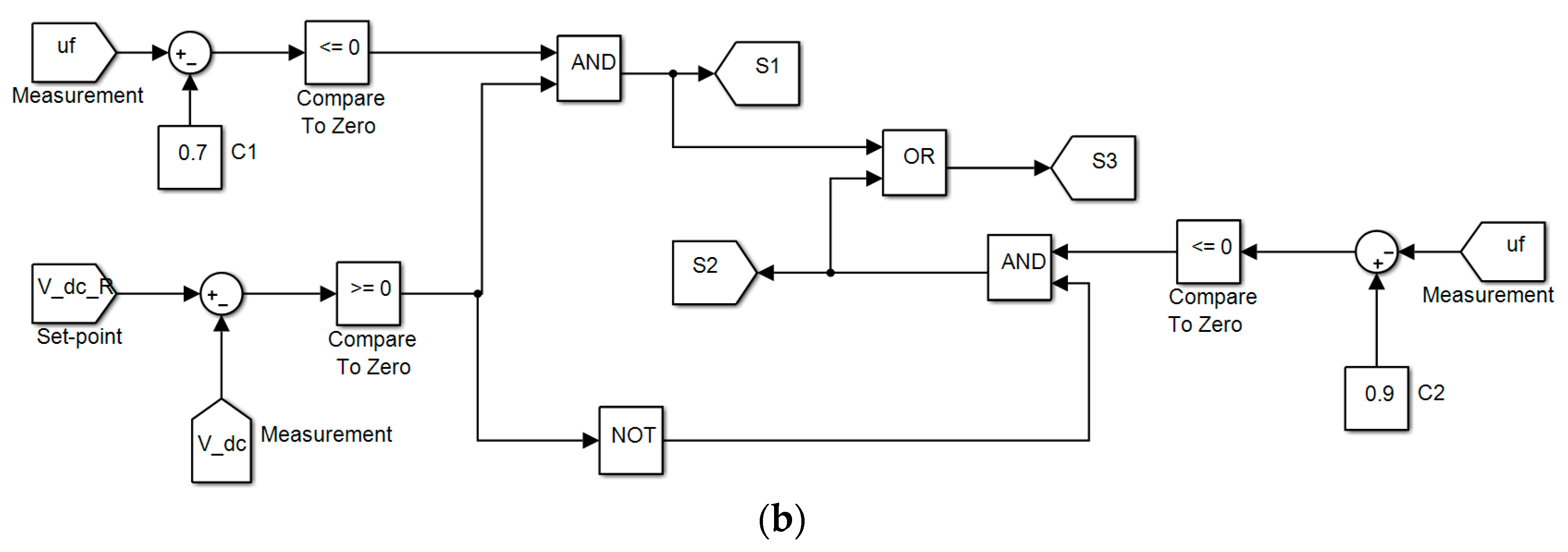
Figure 8.
The comparison of simulation results of the proposed control structure and MPC under the nominal and perturbed condition. (a) MPC under nominal condition; (b) MPC under perturbed; (c) The proposed control under nominal condition; (d) The proposed control under perturbed condition.
Figure 8.
The comparison of simulation results of the proposed control structure and MPC under the nominal and perturbed condition. (a) MPC under nominal condition; (b) MPC under perturbed; (c) The proposed control under nominal condition; (d) The proposed control under perturbed condition.

Figure 9.
The comparison of simulation results of the proposed control structure and MPC in the presence of sensor noise and parameter perturbation. (a) MPC; (b) The proposed control structure.
Figure 9.
The comparison of simulation results of the proposed control structure and MPC in the presence of sensor noise and parameter perturbation. (a) MPC; (b) The proposed control structure.

Table 1.
Nominal Parameters in the SOFC system.
| Parameter | Value | Unit | Representation |
|---|---|---|---|
| 1237 | Absolute temperature | ||
| 96,485 | Faraday’s constant | ||
| 8.314 | Universal gas constant | ||
| 1.18 | Ideal standard potential | ||
| 384 | Number of cells in series in the stack | ||
| 0.996 × 10⁻³ | Constant | ||
| 8.32 × 10⁻⁶ | Valve molar constant for hydrogen | ||
| 2.77 × 10⁻⁶ | Valve molar constant for water | ||
| 2.49 × 10⁻⁵ | Valve molar constant for oxygen | ||
| 26.1 | Response time of hydrogen flow | ||
| 78.3 | Response time of water flow | ||
| 2.91 | Response time of oxygen flow | ||
| 1.145 | Ratio of hydrogen to oxygen | ||
| 0.126 | Ohmic loss | ||
| 5 | Time constant of the fuel processor | ||
| 0.05 | Tafel constant | ||
| 0.11 | Tafel slope | ||
| 800 | Limiting current density |
© 2017 by the authors. Licensee MDPI, Basel, Switzerland. This article is an open access article distributed under the terms and conditions of the Creative Commons Attribution (CC BY) license (http://creativecommons.org/licenses/by/4.0/).
Share and Cite
MDPI and ACS Style
Sun, L.; Hua, Q.; Shen, J.; Xue, Y.; Li, D.; Lee, K.Y. A Combined Voltage Control Strategy for Fuel Cell. Sustainability 2017, 9, 1517. https://doi.org/10.3390/su9091517
AMA Style
Sun L, Hua Q, Shen J, Xue Y, Li D, Lee KY. A Combined Voltage Control Strategy for Fuel Cell. Sustainability. 2017; 9(9):1517. https://doi.org/10.3390/su9091517
Chicago/Turabian StyleSun, Li, Qingsong Hua, Jiong Shen, Yali Xue, Donghai Li, and Kwang Y. Lee. 2017. "A Combined Voltage Control Strategy for Fuel Cell" Sustainability 9, no. 9: 1517. https://doi.org/10.3390/su9091517
Note that from the first issue of 2016, this journal uses article numbers instead of page numbers. See further details here.