Effect of Land-Use Change on the Urban Heat Island in the Fukuoka–Kitakyushu Metropolitan Area, Japan


Department of Environmental Design, Faculty of Design, Kyushu University, 4-9-1 Shiobaru, Minami-ku, Fukuoka 815-8540, Japan
Sustainability 2017, 9(9), 1521; https://doi.org/10.3390/su9091521
Submission received: 30 June 2017
/
Revised: 19 August 2017
/
Accepted: 23 August 2017
/
Published: 26 August 2017
(This article belongs to the Special Issue Urban Heat Island)
Abstract
:In coastal cities, the effect of the sea breeze in mitigating the urban heat island (UHI) phenomenon has attracted attention. This study targeted the Fukuoka–Kitakyushu metropolitan area, the fourth largest metropolitan area in Japan which is also coastal. Doppler Light Detection And Ranging (LiDAR) observations were conducted in the summer of 2015 to clarify the transition of the wind field over the targeted area. To investigate the effects on the UHI of land-use change related to urbanization, the National Land Numerical Information (NLNI) land-use datasets for Japan in 1976 (NLNI-76) and 2009 (NLNI-09) were used in the Weather Research and Forecasting (WRF) model. The results of the simulation showed that most of the northern part of the Kyushu region became warmer, with an average increase of +0.236 °C for the whole simulation period. Comparing the two simulations and the Doppler LiDAR observations, the simulation results with the NLNI-09 dataset (for the year closest to the study period in 2015) showed closer conformity with the observations. The results of the simulation using NLNI-76 showed faster sea breeze penetration and higher wind velocity than the observations. These results suggest that the land-use change related to urbanization weakened the sea breeze penetration in this area.
1. Introduction
Japan is a mountainous island nation most of whose large cities are located in coastal areas and many of which are facing problems caused by urbanization. The urban heat island (UHI) phenomenon is a typical environmental problem encountered in dense urban areas in summer. The effect of the sea breeze in mitigating the UHI phenomenon has attracted attention in coastal cities, making further investigation of the environment of coastal urban areas important.
This study targeted the Fukuoka–Kitakyushu metropolitan area for investigation. This is the fourth largest metropolitan area after Tokyo, Osaka, and Nagoya, all of which are also coastal cities. Within these areas, sea breezes are important factors that mitigate the air-temperature rise during the summer. However, ongoing urbanization could be changing not only the mechanism of the energy balance on urban surfaces, but also the sea breeze system in large coastal cities.
The Fukuoka–Kitakyushu metropolitan area comprises the cities of Fukuoka and Kitakyushu in the Fukuoka prefecture located in the Kyushu region. The heat island monitoring report [1] indicated that the rise in annual average air temperature statistically derived with the linear least squares method from 1931 to 2014 in Fukuoka, in the central part of the targeted area, at 3.1 °C per century, was the second largest after that in Tokyo, at 3.2 °C per century. Moreover, the rise in minimum summer air temperature statistically derived with the linear least squares method from 1931 to 2014 in Fukuoka was the largest, at 3.9 °C per century.
To clarify the effects of land-use change related to urbanization in the Fukuoka–Kitakyushu metropolitan area, a meso-scale meteorological model was utilized. The term “meso” means intermediate between “macro” and “micro”, and in the meteorological field, meso-scale means from a few kilometers to several hundred kilometers. To analyze the UHI in terms of meso-scale phenomena, e.g., motion of the atmosphere, heat transfer between land surface and atmosphere, solar radiation and infrared radiation and so on, meso-scale meteorological models are utilized. The Weather Research and Forecasting model (WRF) [2] developed by the National Center for Atmospheric Research (NCAR) in Boulder, CO, USA, is a meso-scale meteorological model that is widely utilized to analyze UHI phenomena. For example, Holt and Pullen analyzed the UHI in the New York City metropolitan area, USA, using the WRF and the Coupled Ocean-Atmosphere Mesoscale Prediction System (COMPAS) [3]. Miao et al. analyzed the UHI and boundary layer structures in Beijing, China, with the WRF [4]. Giannaros et al. investigated the spatial and temporal structure of the UHI in Athens, Greece, with the WRF [5]. In Japan, Kusaka et al. utilized the WRF to evaluate the effect of future global warming in the Tokyo, Osaka, and Nagoya metropolitan areas [6]. Hisada et al. investigated the relationship between the characteristics of sea breeze and land use in the Fukuoka metropolitan area using the WRF [7]. To evaluate the effect of land-use change, the WRF is also adopted in this study.
The National Land Numerical Information (hereafter referred to as NLNI) land-use datasets provided by the National Land Information Division, National Spatial Planning and Regional Policy Bureau, Ministry of Land, Infrastructure, Transport and Tourism (MLIT) of Japan [8] were used to represent the land-use change in the Fukuoka–Kitakyushu metropolitan area, using a Land Surface Model (LSM) with the mosaic option in the WRF. The NLNI land-use datasets were published for several years, with the earliest dataset published in 1976 and the latest published in 2009. These were adopted to represent the land-use change over about three decades. The investigation period was set in the summer of 2015. To clarify the effect of land-use change, the same meteorological and simulation conditions were applied to the two simulation cases, except for the land-use fraction dataset.
Additionally, upper air observations using Doppler Light Detection And Ranging (LiDAR) were conducted to clarify the transition of the wind field over the Fukuoka–Kitakyushu metropolitan area. The Doppler LiDAR system emits laser pulses to the atmosphere and detects the reflected light back-scattered from aerosols. Wind velocity along the line of sight is then obtained using the Doppler frequency shifts from the back-scattered light. In the field of urban climate, Doppler LiDAR systems are utilized to observe wind profiles over urban areas. For example, Lane et al. [9] and Drew et al. [10] observed wind profiles over central London, UK. In the Tokyo metropolitan area, some research on sea breezes flowing over the urban area has been conducted using upper air observations. For example, Yoshikado and Kondo carried out large-scale upper air observations using radiosondes and pilot balloons, to clarify the transportation of atmospheric pollutants affected by the sea breeze from Tokyo Bay in the 1980s [11]. Following that study, the present author conducted upper air observations using two sets of Doppler LiDAR in 2011 [12]. One instrument was set at approximately 12 km from the coastline of Tokyo Bay, and the other was set at approximately 34 km from the coastline. These sets of Doppler LiDAR observations captured the sea breeze penetration from Tokyo Bay. In 2012, Yoshikado et al. [13] carried out upper air observations using Global Positioning System (GPS) sondes and clarified the thermal structure over the Tokyo metropolitan area in summer. In the Fukuoka–Kitakyushu metropolitan area, this kind of upper air observation that focuses on the urban climate has been limited. For example, Hisada et al. [14] observed wind fields over Fukuoka city using Doppler SODAR (SOnic Detection And Ranging); however, compared with the Tokyo metropolitan area, the accumulation of observation data is not sufficient. Therefore, to clarify the transition of the wind field over the Fukuoka–Kitakyushu metropolitan area, Doppler LiDAR observations were conducted simultaneously with the numerical simulations.
2. Materials and Methods
2.1. Outline of the Meso-Scale Meteorological Model
The WRF ver. 3.7.1 was used to analyze the atmospheric conditions of the targeted area, and a mosaic land-use categories option for the Noah LSM was incorporated from the WRF ver. 3.6 [15]. In the previous LSM, the land surface property of each analysis cell was defined by the dominant land-use category. If one analysis cell consisted of 60% “urban” land-use and 40% “forest” land-use, that cell was defined as “urban”, and the characteristics of a forest were neglected. However, the mosaic LSM enables the representation of different land-use fractions in each analysis cell. In an already urbanized area, the amount of further conversion from other land uses to “urban” within a short time period may be small. Therefore, the mosaic LSM is useful in analyzing urban climate transitions caused by land-use change over several decades, which is not represented by the dominant land-use.
2.2. Outline of the National Land Numerical Information Land-Use Datasets
In this study, the NLNI land-use datasets were used to represent the progress of land-use change. To make the NLNI land-use datasets suitable for the WRF LSM, the WRF Preprocessing System (WPS) was modified [16]. The NLNI land-use datasets were published in 1976, 1987, 1991, 1997, 2006 and 2009. From these, the datasets that were published in 1976 (earliest) and 2009 (latest) were used in this study. The NLNI land-use datasets are stored on the basis of the Basic Grid Square (Third Area Partition) with a resolution of approximately 1 km2 and a grid spacing with latitude and longitude of 30″ and 45″, respectively. The Basic Grid Square is widely used for statistics regarding population, land-use, and urban planning, among others, by national and local governments in Japan. A resolution of approximately 1 km2 is suitable as input data for the meso-scale model. Each Basic Grid Square has fractional land-use data with different categories by year. Since each dataset comprised different land-use categories, the original ones were re-grouped into six categories of land-use to adapt to the WRF, as shown in Table 1. In the WRF model, the land-use dataset provided by the U.S. Geological Survey (USGS) (Reston, VA, USA) is used as the default.
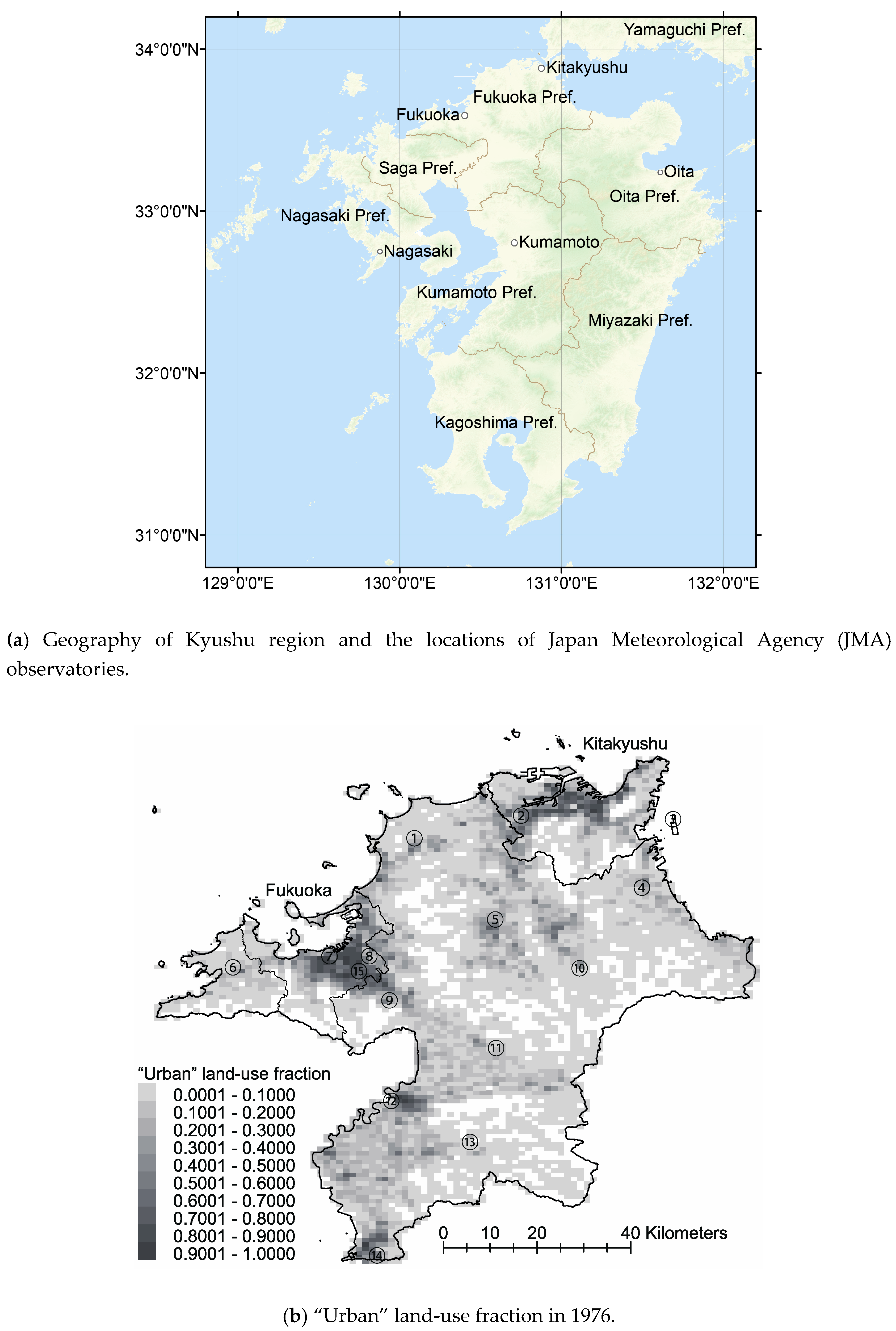
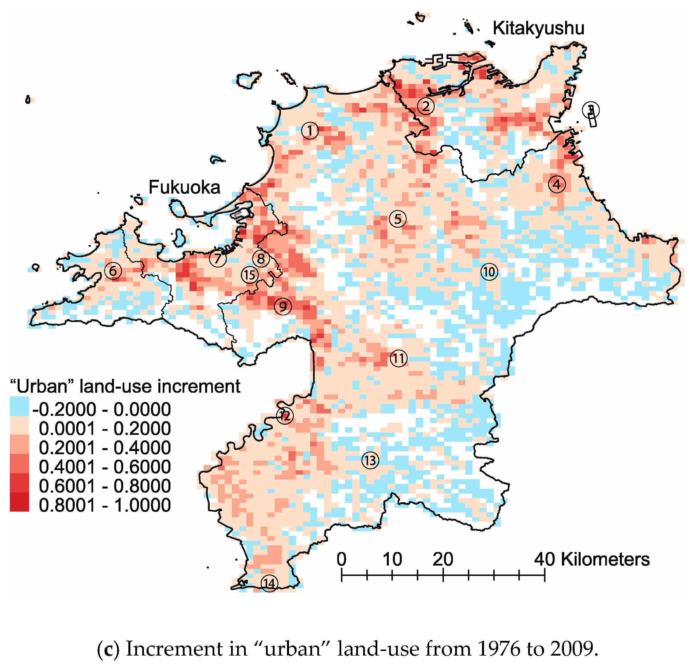
Figure 1a shows the geography of the Kyushu region, the main target of this study. Figure 1b shows the fraction of land in the “urban” category (shaded in Table 1) in the Fukuoka prefecture in 1976. The resolution of the figure is 1 km, and the degree of shading indicates the fraction of “urban” land-use within each 1 km2 cell. Figure 1c shows the increment in the “urban” land-use fraction over time. “Urban” land-use fractions in 1976 were subtracted from those in 2009; so that a positive value (red in Figure 1c) indicates an increase in “urban” land-use in that cell. Overall, the results obtained over the three decades did not show extremely rapid land-use change in the Fukuoka–Kitakyushu metropolitan area. In particular, the increments in “urban” land-use in the central part of Fukuoka city were very small, because this area had already been extensively urbanized by the 1970s. However, the “urban” land-use area had increased in the surrounding areas due to urban expansion.
2.3. Analysis Conditions
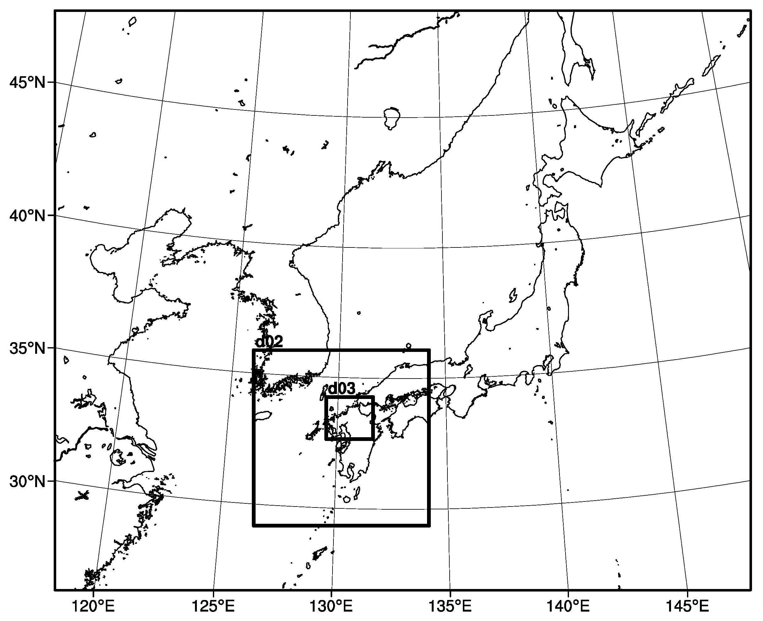
Figure 2 illustrates the analysis domains, which covered an area of 3000 km (east–west) × 2500 km (south–north) with a horizontal resolution of 25 km. The entire analysis domain was two-way nested into two-fold sub-domains: domain 2 (750 × 750 km with a resolution of 5 km) and domain 3 (200 × 180 km with a resolution of 1 km). The vertical domain was divided into 48 unequally spaced grids. The top was set by pressure at 5000 Pa (approximately 20 km in height), and the lowest grid height was approximately 25 m.
The summer of 2015 was selected as the study period. The simulations were started on 24 July, and the time integration was performed for 69 days. The first 15 days were for spin-up, and the results of the hourly output data for 54 days, from 8 August to 30 September 2015, were used in this study. This evaluation period covered the upper air observation period. The initial conditions were obtained from the National Centers for Environmental Prediction Final operational global analysis data (NCEP FNL), with a resolution of 0.25°. Relaxation lateral boundary conditions were applied to domain 1, and nest lateral boundary conditions were applied to domains 2 and 3. The surface temperature and the sea surface temperature, for setting the lower boundary conditions, were obtained from the NCEP FNL data. In this study, the following schemes were applied for all domains and all cases: microphysics: Thompson scheme [17]; long-wave radiation: Rapid Radiative Transfer Model (RRTM) scheme [18]; short-wave radiation: Goddard scheme [19]; surface layer: Eta similarity scheme based on Monin–Obukhov similarity [20]; land surface: Noah LSM model [21] with mosaic option [16]; and planetary boundary layer: Mellor–Yamada–Janjic scheme [20]. Grell 3D ensemble cumulus parameterization [22] was applied only for domain 1. Urban canopy models were not applied for all domains because of the lack of detailed building parameters. Therefore, the effect of urbanization was represented by urban land-use, and the transition of urban morphology could not be considered.
To evaluate the climatological effect of land-use changes over the three decades, numerical simulations were performed using two different land-use datasets. For simplicity, these two datasets are abbreviated as NLNI-76 for the National Land Numerical Information land-use dataset for 1976, and NLNI-09 for 2009. In order to evaluate the influence of the land-use datasets, the same meteorological data were adopted as the initial conditions for both cases. Furthermore, to evaluate the effects of the mosaic LSM and NLNI land-use dataset, a USGS land-use dataset, used in the WRF by default, was also adopted. For the USGS dataset only, the Noah LSM model without the mosaic option was adopted, with the other settings remaining the same as for NLNI-76 and NLNI-09.
2.4. Outline of the Doppler LiDAR System
For the observations, the Leosphere WINDCUBE V2 Doppler LiDAR system was set up at the Ohashi campus of Kyushu University (33.5597° N 130.4308° E), approximately 6 km from the coastline, with a height of 8 m above ground level (AGL). The location of the Doppler LiDAR observation site is shown as no. 15 in Figure 1b,c.
The Leosphere WINDCUBE V2 Doppler LiDAR system emits eye-safe pulsed laser beams at fixed angles; four beams with zenith angles of 28° facing to the north, east, south and west respectively, and one vertical beam. The wind speed range is from 0 to 60 m/s and the resolution is 0.1 m/s. The wind direction resolution is 2°. The vertical resolution of the Doppler LiDAR is 20 m, and the range is from 40 m to 260 m. The data sampling rate is 1 Hz. In this study, measurements were averaged over 10-min intervals.
3. Results and Discussion
3.1. Comparing Observation and Simulation Results of the Surface Air Temperature
The NLNI-09 utilized the latest land-use dataset, from the year (2009) closest to the simulation period in 2015. Therefore, to validate the simulation performance, the results of the NLNI-09 simulation were compared first with the observation data provided by the Japan Meteorological Agency (JMA). To evaluate the effects of the mosaic LSM and the different land-use datasets, the results of the USGS case were also compared. In Fukuoka prefecture, the surface air temperatures at 14 sites were observed. The locations of the observation sites are shown in Figure 1b,c. Table 2 shows the mean error (ME) and root mean square error (RMSE) for the observed surface air temperatures and simulated air temperatures at 2 m AGL. The data for evaluation were hourly data for 54 days from 8 August to 30 September 2015. The domain used for this evaluation was domain 3, with a resolution of 1 km.
The ME of the NLNI-09 simulation for the 14 sites was slightly positive (+0.128), while the ME of the USGS simulation for the 14 sites was negative (−0.731). These differences suggest that the USGS land-use dataset was unable to represent the urban area in the targeted area correctly. Table 3 shows the land-use fractions in the NLNI-09 dataset, and the dominant land-use categories in the USGS dataset, for the 14 grid cells with a resolution of 1 km that include the JMA observation sites. Comparing the NLNI-09 and USGS simulations, the dominant land-use categories in the NLNI-09 and the USGS datasets showed non-conformity. The USGS simulation underestimated the area of urban land-use.
The RMSE of the NLNI-09 simulation ranged from 2.553 to 3.473, and the average of the 14 sites was 3.247. The RMSE of the USGS simulation ranged from 2.979 to 3.748, and the average of the 14 sites was 3.391. The NLNI-09 simulation showed better results; however, the difference was small. These results suggest that significant errors occurred in the numerical simulation. Further investigation of these simulation errors is needed.
Hereafter, the results of the NLNI-76 and NLNI-09 simulations are discussed, to consider the effect of land-use change on the urban climate of the Fukuoka–Kitakyushu metropolitan area.
3.2. Surface Air Temperature Change Caused by Land-Use Change
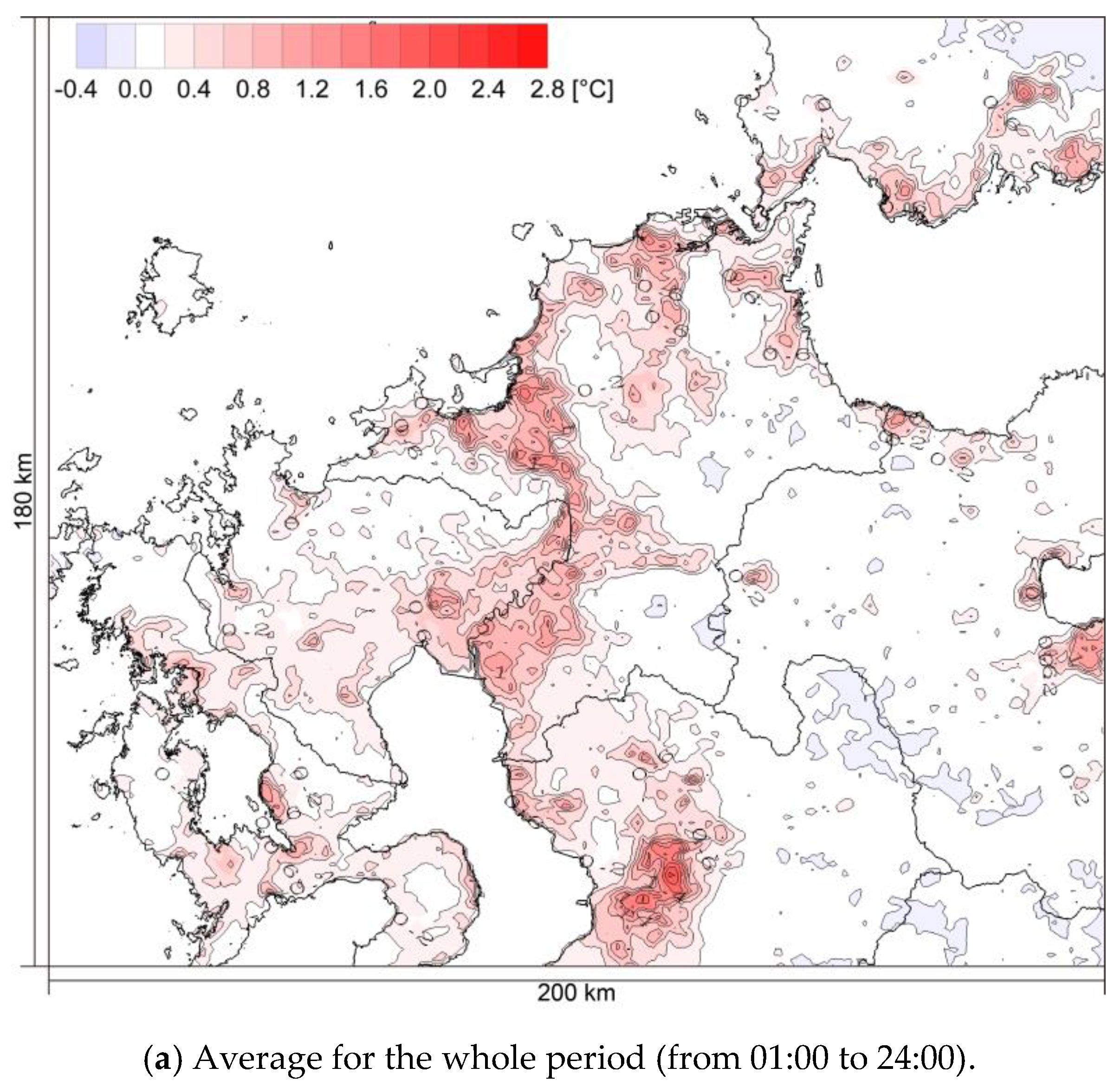
Figure 3 shows the difference in air temperature at 2 m AGL between the NLNI-76 and NLNI-09 simulations. The hourly air temperature data for the 54 days from 8 August to 30 September 2015 were averaged for the land surface only. The average air temperatures for the NLNI-76 simulation were subtracted from those of the NLNI-09 simulation. Negative values (blue tones in Figure 3) indicated that the air temperature in NLNI-76 was higher than that in NLNI-09, and positive values (red tones in Figure 3) indicated that the air temperature in NLNI-76 was lower than that in NLNI-09.
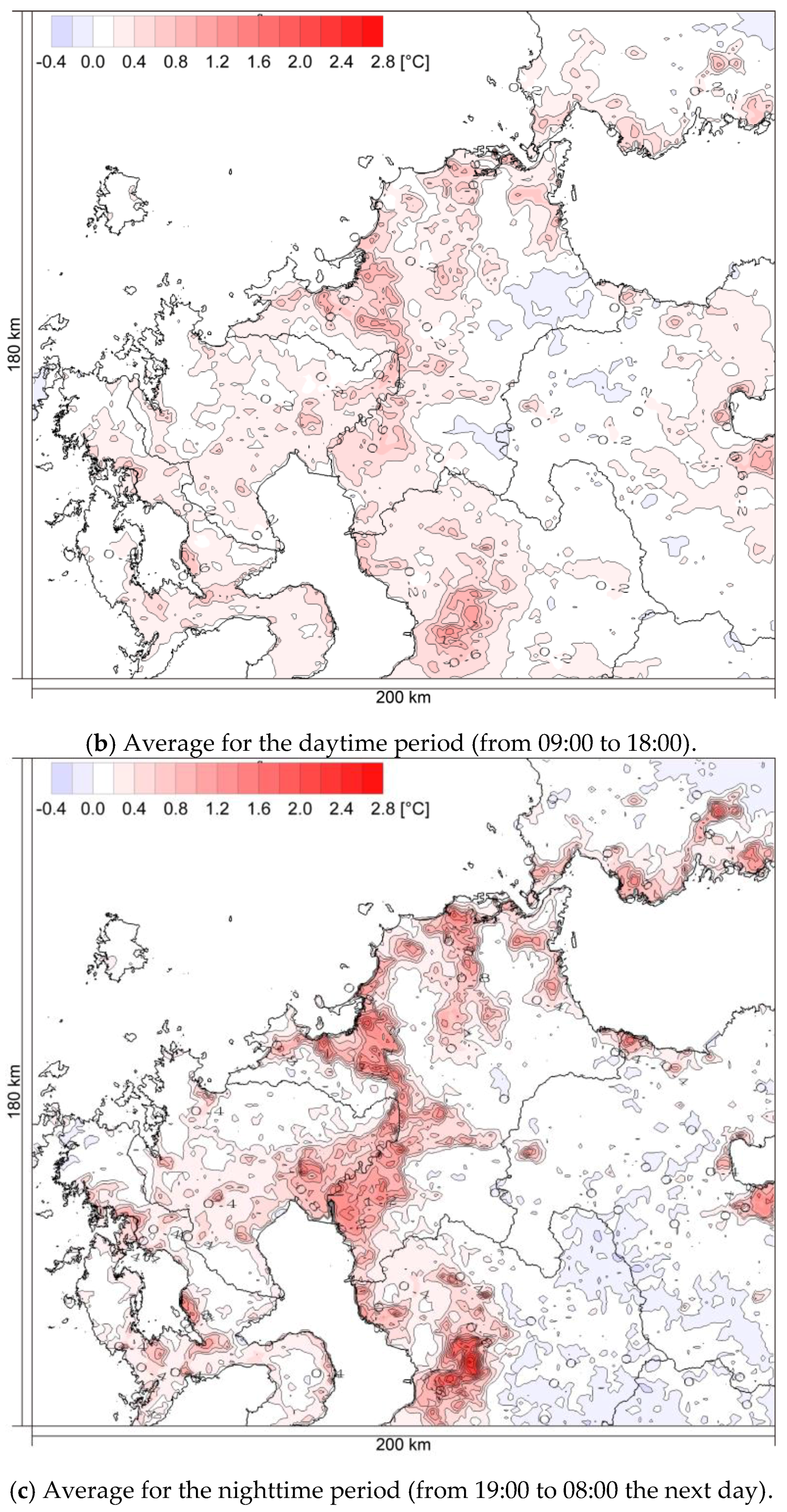
As mentioned above, the central parts of Fukuoka and Kitakyushu (the darker colors in Figure 1b) were already urbanized in the 1970s, so the air temperature increases caused by land-use change in these areas have been small. However, because of urban expansion, the urban heat island phenomenon has expanded. Although some areas in Figure 3a show decreases in the air temperature, the air temperature difference averaged over the land surface of domain 3 for the whole period was an increase of +0.236 °C. Figure 3b,c shows the temperature rise in daytime and nighttime periods, in the same manner as Figure 3a. The temperature rise averaged over the land surface of domain 3 in the nighttime was +0.245 °C, which is larger than the daytime average of +0.225 °C. Moreover, the nighttime range, with a minimum value of −0.324 and a maximum value of +2.656 °C, is wide compared to the daytime range, which has a minimum value of −0.144 and a maximum value of +1.317 °C.
3.3. Transition of the Sea Breeze over the Urban Area
Sea breeze circulation is driven by the air pressure difference between the land and the sea surfaces, caused by the temperature difference between these surfaces. The temperature difference is caused by solar radiation. Therefore, the sea breeze circulation is clearly observed on clear days with a small synoptic scale pressure gradient. During the observation period, 11 September 2015 gave the best conditions to observe the sea breeze blowing across the urban area. On that day, the cloud cover was less than 1 okta for a whole day, and the pressure gradients were small. The gradient of mean sea level pressure between the Fukuoka district meteorological observatory and the Kumamoto local meteorological observatory was 0.7 hPa, with a distance of approximately 90 km in the north–south direction; and the gradient of mean sea level pressure between the Oita local meteorological observatory and the Nagasaki local meteorological observatory was 0.2 hPa, with a distance of approximately 170 km in the east–west direction. The locations of observatories are shown in Figure 1a.
The Doppler LiDAR observation site was located approximately 6 km from the coastline of Hakata Bay in a south-southeast direction. Therefore, in this study, the sea breeze was defined as a northerly wind ranging from the west-northwest to the north-northeast, with an average velocity of 2 m/s or greater based on the Doppler LiDAR observations at 12 heights from 40 m to 260 m with a vertical resolution of 20 m.
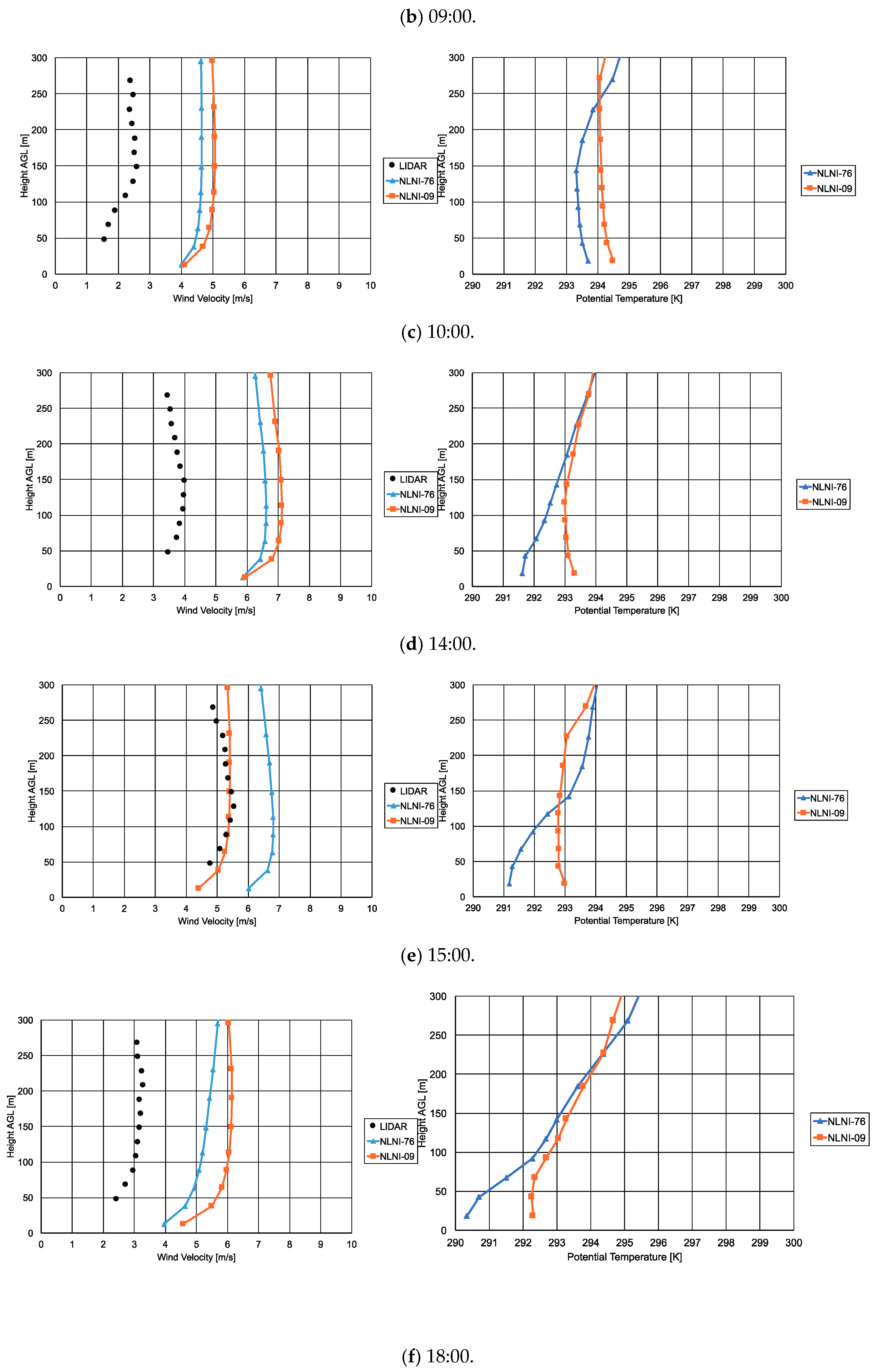
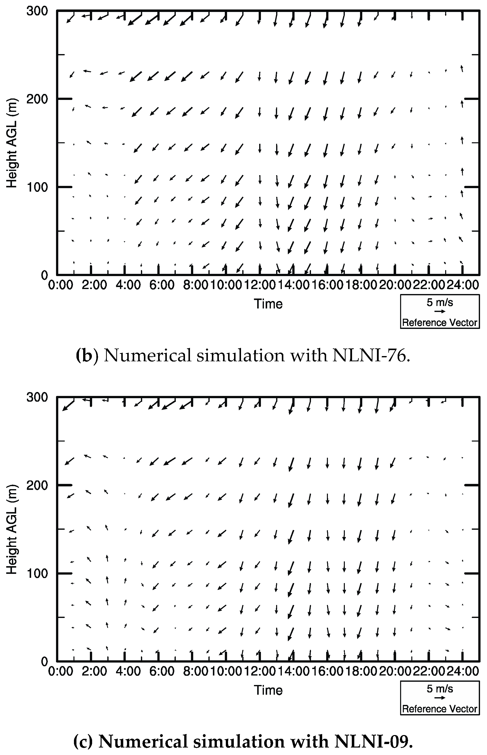
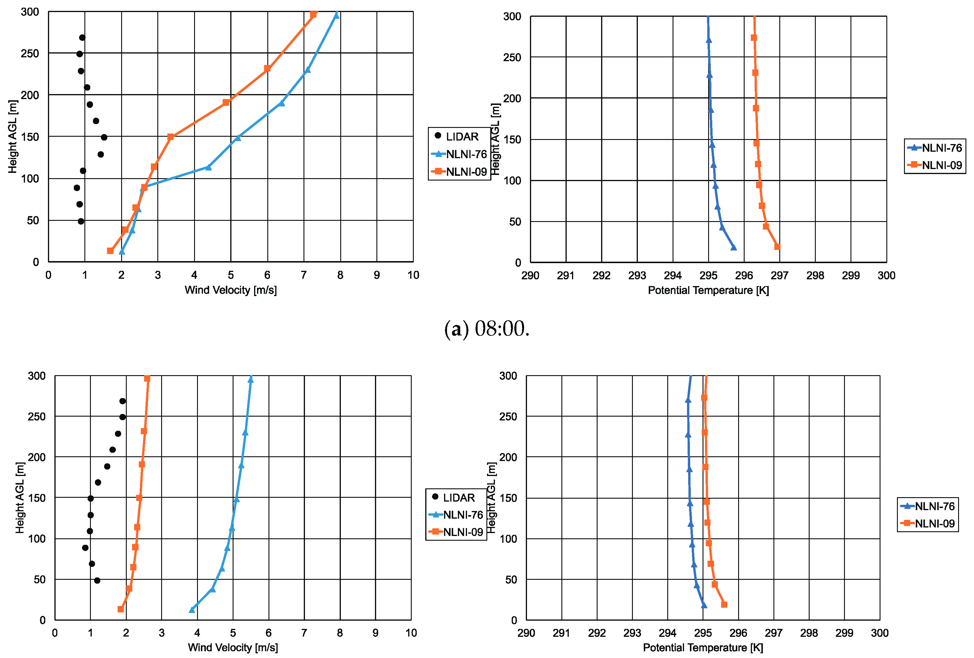
Figure 4 shows the time-height cross sections of the horizontal wind vectors of the Doppler LiDAR observations, and the numerical simulations with the NLNI-76 and the NLNI-09 land-use datasets, on 11 September 2015. The observation results were averaged over 10-minute intervals. Figure 5 shows vertical wind and potential temperature profiles at selected times. Here, the potential temperature is the temperature of an air parcel which changed adiabatically from its initial state to the standard pressure, 1000 hPa. Because the air temperature is affected by the air pressure, to investigate the thermal structures in the vertical direction, the potential temperature is an important parameter.
Figure 4a,c shows that the Doppler LiDAR captured sea breeze penetration at 10:00 and the simulation results for the NLNI-09 dataset showed the same tendency, although the wind directions were not accurate. The results of the NLNI-76 predicted sea breeze penetration at 09:00 are given in Figure 4b. Figure 5a shows vertical profiles at 08:00, before the sea breeze blows into the Ohashi Doppler LiDAR observation site. Vertical wind profiles at 09:00 in Figure 5b clearly show the difference between the Doppler LiDAR, the NLNI-76 simulation, and the NLNI-09 simulation. At 10:00, in Figure 5c, the Doppler LiDAR captured the sea breeze penetration. At the same time, the vertical wind profile of the NLNI-09 simulation showed higher velocity. At 14:00, in Figure 5d, the simulation with NLNI-76 showed a potential temperature drop below 50 m AGL, and the simulation with NLNI-09 showed a higher wind velocity than NLNI-76. At 15:00, in Figure 5e, the sea breeze with the highest velocity was observed, and the NLNI-09 simulation showed good agreement with the observations. On the other hand, the NLNI-76 simulation showed a higher velocity than the Doppler LiDAR and NLNI-09 results. Moreover, the potential temperature profile of NLNI-76 showed an inversion below 150 m AGL. At 18:00, in Figure 5f, the potential temperature profiles showed a large difference between NLNI-76 and NLNI-09 below 100 m AGL.
Although the NLNI-09 simulation showed good agreement with the Doppler LiDAR observations at 15:00 (Figure 5e), generally, the numerical simulations overestimated the wind velocities near the land surface. Moreover, the wind directions of simulations were not accurate compared with the Doppler LiDAR observations. One possible reason is that an urban canopy model was not utilized in this study; therefore, the simulation results underestimated the friction caused by urban morphology.
Comparing the two simulation results, the NLNI-09 simulation, which is the more urbanized case, showed lower wind velocity and later sea breeze penetration than the NLNI-76 simulation. The results of this study suggest that the land-use change related to urbanization has delayed sea breeze penetration and weakened its wind velocity. However, this result partially contradicts previous researches. Yoshikado [23,24] investigated the relationship between UHI and sea breeze using a two-dimensional hydrostatic boundary-layer model, and summarized that the UHI delays the inland penetration of the sea breeze, and that in coastal regions the UHI intensifies the sea breeze velocity during its growing stage. Kusaka et al. [25] utilized a hydrostatic three-dimensional model to analyze land-use change in the Tokyo metropolitan area, and summarized that the progress of urbanization delays the sea breeze penetration from Tokyo Bay and makes the wind velocity of the sea breeze stronger in the inland area. Our previous study [26] in the Tokyo metropolitan area, using the meso-scale meteorological model MM5 [27], showed the delay of sea breeze penetration from Tokyo Bay to the inland area; however, the difference of wind velocity in the inland area was not significant. In this study, comparing NLNI-76 with NLNI-09, the increase in the UHI is shown to delay sea breeze penetration. This result is consistent with previous studies [23,24,25,26]. Meanwhile, the increase in the UHI has weakened the velocity of the sea breeze.
In this study, the simulation results of the WRF overestimated the wind velocities near the land surface. The possible reasons of these errors are uncertainties about the analysis model and the initial conditions. In terms of the model uncertainty, as mentioned above, the urban canopy model was not utilized in this study, and it was possible for the analysis model to underestimate the friction caused by urban morphology. On the other hand, it was also possible for the uncertainty of the initial conditions to cause these errors. To utilize the meso-scale meteorological models such as the WRF, the initial conditions are obtained from global analysis data such as the NCEP FNL data; and these regular, gridded global analysis data are produced from discretely distributed observations on Earth. In this process, uncertainty in the initial conditions of the meso-scale meteorological models cannot be avoided. Lorenz showed that very small differences in the initial conditions will cause errors in weather prediction over time [28,29]. One way of reducing the uncertainties in the initial conditions is an ensemble simulation; however, the ensemble simulation needs a number of simulations with perturbations of initial conditions. As with the initial conditions, a multi-model ensemble simulation is one way to reduce the uncertainties of the model. In this study, evaluating the effect of urbanization on sea breeze penetration quantitatively is difficult because of the uncertainties of the model and initial conditions; therefore, what are shown here are the results of qualitative comparison. Further investigations are needed, with the ensemble simulations using various conditions and various models for various urban areas, in order to clarify the effect of land-use change on sea breeze circulation.
4. Conclusions
This study investigated the Fukuoka–Kitakyushu metropolitan area, which is the fourth largest metropolitan area in Japan. Compared with the Tokyo metropolitan area, the capital of Japan and the largest metropolitan area in the world, the number of urban climate studies in the targeted area is limited. Therefore, to accumulate data on the urban climate in the Fukuoka–Kitakyushu metropolitan area, numerical simulations with a meso-scale meteorological model (the WRF) and upper air observations using Doppler LiDAR were carried out simultaneously in the summer of 2015. For the numerical simulation, the NLNI land-use fraction datasets for Japan were used to represent the progress of land-use changes, in place of the default USGS land-use dataset in the WRF.
For simulation results of the surface air temperature, the results using the NLNI land-use dataset for 2009 showed fewer errors, when compared to the observations by JMA, than those using the USGS land-use dataset. This comparison suggested that the USGS land-use dataset was unable to represent the urban area precisely.
To consider the effect of land-use changes over three decades on the urban climate of the targeted area, the NLNI land-use datasets for 1976 and 2009 were utilized in the WRF simulations with the mosaic LSM. Based on the surface air temperature, most of the northern part of the Kyushu region became warmer because of land-use change related to urbanization, with an average increase over the land surface of +0.236 °C for the whole simulation period. The temperature increases in the areas surrounding Fukuoka city and Kitakyushu city were significant because of the urban expansion. It is possible that the land-use changes in the Fukuoka–Kitakyushu metropolitan area also had an effect on the sea breeze penetration from Hakata Bay to Fukuoka city. Comparing the two simulation results and the Doppler LiDAR observations, the simulation results using the NLNI-09 dataset (for the year closest to the study period in 2015) showed greater agreement with the observations. The results of the NLNI-76 simulation showed faster sea breeze penetration and higher wind velocity compared with the observations. These results suggest that the land-use changes have weakened sea breeze penetration. However, this tendency partially contradicts other research. To expand the knowledge base for the mitigation of urban heat island phenomena by sea breezes in coastal cities in the summer, additional investigations are needed and it will be necessary to reduce the uncertainties of the simulations used.
Acknowledgments
This work was supported by the Japan Society for the Promotion of Science Grant-in-Aid for Young Scientists (A) (Grant Number: 25709053). The Doppler LiDAR system was borrowed from EKO Instruments. I would like to express my gratitude to them.
Author Contributions
The author designed the study, analyzed and interpreted the data, and wrote the manuscript. The author approved the final version of the manuscript, and agree to be accountable for all aspects of the work in ensuring that questions related to the accuracy or integrity of any part of the work are appropriately investigated and resolved.
Conflicts of Interest
The author declares no conflict of interest.
References
- Japan Meteorological Agency. Heat Island Monitoring Report 2014. Available online: http://www.data.jma.go.jp/cpdinfo/himr/2014/index.html (accessed on 15 January 2017). (In Japanese)
- Skamarock, W.C.; Klemp, J.B.; Dudhia, J.; Gill, D.O.; Barker, D.M.; Duda, M.G.; Huang, X.Y.; Wang, W.; Powers, J.G. A Description of the Advanced Research WRF Version 3. NCAR Tech. Note 2008, 468, 88. [Google Scholar]
- Holt, T.; Pullen, J. Urban canopy modeling of the New York City metropolitan area: A comparison and validation of single-and multilayer parameterizations. Mon. Weather Rev. 2007, 135, 1906–1930. [Google Scholar] [CrossRef]
- Miao, S.; Chen, F.; LeMone, M.A.; Tewari, M.; Li, Q.; Wang, Y. An Observational and Modeling Study of Characteristics of Urban Heat Island and Boundary Layer Structures in Beijing. J. Appl. Meteorol. Climatol. 2009, 48, 484–501. [Google Scholar] [CrossRef]
- Giannaros, T.M.; Melas, D.; Daglis, I.A.; Keramitsouglou, I.; Kourtidis, K. Numerical study of the urban heat island over Athens (Greece) with the WRF model. Atmos. Environ. 2013, 73, 103–111. [Google Scholar] [CrossRef]
- Kusaka, H.; Hara, M.; Takane, Y. Urban Climate Projection by the WRF Model at 3-km Horizontal Grid Increment: Dynamical Downscaling and Predicting Heat Stress in the 2070’s August for Tokyo, Osaka, and Nagoya Metropolises. J. Meteorol. Soc. Jpn. 2012, 90B, 47–63. [Google Scholar] [CrossRef]
- Hisada, Y.; Uechi, T.; Matsunaga, N. A relationship between the characteristics of sea breeze and land-use in Fukuoka Metropolitan area. In Proceedings of the 7th International Conference on Urban Climate, Yokohama, Japan, 2 July 2009. [Google Scholar]
- National Land Information Division, National Spatial Planning and Regional Policy Bureau, MLIT of Japan. National Land Numerical Information Download Service. Available online: http://nlftp.mlit.go.jp/ksj-e/index.html (accessed on 15 January 2016).
- Lane, S.E.; Barlow, J.F.; Wood, C.R. An assessment of a three-beam Doppler lidar wind profiling method for use in urban areas. J. Wind Eng. Ind. Aerodyn. 2013, 119, 53–59. [Google Scholar] [CrossRef]
- Drew, D.R.; Barlow, J.F.; Lane, S.E. Observations of wind speed profiles over Greater London, UK, using a Doppler lidar. J. Wind Eng. Ind. Aerodyn. 2013, 121, 98–105. [Google Scholar] [CrossRef]
- Yoshikado, H.; Kondo, H. Inland penetration of the sea breeze over the suburban area of Tokyo. Boudary Layer Meteorol. 1989, 48, 389–407. [Google Scholar] [CrossRef]
- Kawamoto, Y. Doppler lidar observations of wind fields over the Tokyo metropolitan area. In Proceedings of the 8th International Conference on Urban Climate, Dublin, Ireland, 6–10 August 2012. [Google Scholar]
- Yoshikado, H.; Nakajima, K.; Kawamoto, Y.; Ooka, R. Heat Budget of Sea Breezes Passing through Urbanized Areas of Tokyo. Tenki 2014, 61, 541–548. (In Japanese) [Google Scholar]
- Hisada, Y.; Oda, Y.; Matsunaga, N. A simulation of sea breeze over Fukuoka Metropolitan are. Proc. Hydraul. Eng. 2008, 52, 235–240. (In Japanese) [Google Scholar] [CrossRef]
- Kawamoto, Y. Effect of urbanization on the urban climate in coastal city, Fukuoka-Kitakyushu metropolitan area, Japan. In Proceedings of the 9th International Conference on Urban Climate, Toulouse, France, 20–24 July 2015. [Google Scholar]
- Li, D.; Bou-Zeid, E.; Barlage, M.; Chen, F.; Smith, J.A. Development and evaluation of a mosaic approach in the WRF-Noah framework. J. Geophys. Res. Atmos. 2013, 118, 11918–11935. [Google Scholar] [CrossRef]
- Thompson, G.; Field, P.R.; Rasmussen, R.M.; Hall, W.D. Explicit Forecasts of Winter Precipitation Using an Improved Bulk Microphysics Scheme. Part II: Implementation of a New Snow Parameterization. Mon. Weather Rev. 2008, 136, 5095–5115. [Google Scholar] [CrossRef]
- Mlawer, E.J.; Taubman, S.J.; Brown, P.D.; Iacono, M.J.; Clough, S.A. Radiative transfer for inhomogeneous atmosphere: RRTM, a validated correlated-k model for the longwave. J. Geophys. Res. 1997, 102, 16663–16682. [Google Scholar] [CrossRef]
- Chou, M.D.; Suarez, M.J.; Liang, X.Z.; Yan, M.M.H. A thermal infrared radiation parameterization for atmospheric studies. NASA Tech. Memo. 2001, 19, 68. [Google Scholar]
- Janjic, Z.I. Nonsingular Implementation of the Mellor–Yamada Level 2.5 Scheme in the NCEP Meso model. NCEP Off. Note 2002, 437, 61. [Google Scholar]
- Tewari, M.; Chen, F.; Wang, W.; Dudhia, J.; LeMone, M.A.; Mitchell, K.; Ek, M.; Gayno, G.; Wegiel, J.; Cuenca, R.H. Implementation and verification of the unified NOAH land surface model in the WRF model. In Proceedings of the 20th Conference on Weather Analysis and Forecasting/16th Conference on Numerical Weather Prediction, Seattle, DC, USA, 22–26 January 2004. [Google Scholar]
- Grell, G.A.; Devenyi, D. A generalized approach to parameterizing convection combining ensemble and data assimilation techniques. Geophys. Res. Lett. 2002, 29, 38-1–38-4. [Google Scholar] [CrossRef]
- Yoshikado, H. Numerical Study of the Daytime Urban Effect and Its Interaction with the Seat Breeze. J. Appl. Meteorol. 1992, 31, 1146–1164. [Google Scholar] [CrossRef]
- Yoshikado, H. Interaction of the Sea Breeze with Urban Heat Islands of Different Sizes and Locations. J. Meteorol. Soc. Jpn. 1994, 72, 139–143. [Google Scholar] [CrossRef]
- Kusaka, H.; Kimura, F.; Hirakuchi, H.; Mizutori, M. The Effects of Land-Use Alteration on the Sea Breeze and Daytime Heat Island in the Tokyo Metropolitan Area. J. Meteorol. Soc. Jpn. 2000, 78, 405–420. [Google Scholar] [CrossRef]
- Kawamoto, Y.; Yoshikado, H.; Ooka, R.; Hayami, H.; Huang, H.; Khiem, M.V. Sea Breeze Blowing into Urban Areas: Mitigation of the Urban Heat Island Phenomenon. In Ventilating Cities: Air-Flow Criteria for Healthy and Comfortable Urban Living; Kato, S., Hiyama, K., Eds.; Springer: Dordrecht, The Netherland, 2012; pp. 11–32. ISBN 978-94-007-2770-0. [Google Scholar]
- Anthes, R.A.; Warner, T.T. Development of hydrodynamic models suitable for air pollution and other mesometeorological studies. Mon. Weather Rev. 1978, 106, 1045–1078. [Google Scholar] [CrossRef]
- Lorenz, E.N. Deterministic Nonperiodic Flow. J. Atmos. Sci. 1963, 20, 130–141. [Google Scholar] [CrossRef]
- Lorenz, E.N. The predictability of a flow which possesses many scales of motion. Tellus 1969, 21, 289–307. [Google Scholar] [CrossRef]
Figure 1.
Geography of targeted area and “urban” land-use fraction in Fukuoka prefecture: (a) The geography of the Kyushu region. The locations of the Fukuoka district meteorological observatory, the Kumamoto local meteorological observatory, the Oita local meteorological observatory and the Nagasaki local meteorological observatory are also shown. (b) The “urban” land-use fraction in 1976. The degree of shading indicates the fraction of “urban” land-use within each grid cell. (c) Increase in the “urban” land-use fraction. The red indicates the degree of increase in the “urban” land-use fraction from 1976 to 2009, and the blue indicates the decrease. Numbers from 1 to 14 enclosed within circles indicate the observation sites of the Japan Meteorological Agency (Tokyo, Japan). Number 15 indicates the Doppler LiDAR observation site.


Figure 2.
Analysis domains for the Weather Research and Forecasting model (WRF) simulation. Domain 1 covers all of Japan, domain 2 covers the entire Kyushu region, and domain 3 covers the northern part of the Kyushu region, which was the main target area in this study.
Figure 2.
Analysis domains for the Weather Research and Forecasting model (WRF) simulation. Domain 1 covers all of Japan, domain 2 covers the entire Kyushu region, and domain 3 covers the northern part of the Kyushu region, which was the main target area in this study.

Figure 3.
Differences in averaged air temperature between NLNI-76 and NLNI-09 over 54 days from 8 August to 30 September 2015. The blue tones show a temperature drop, and the red tones show a temperature rise from NLNI-76 to NLNI-09: (a) Difference in averaged air temperature for the whole period. The spatial average for this domain is +0.236 °C, with a minimum value of −0.171 °C and a maximum value of +2.049 °C. (b) Difference in averaged air temperature for the daytime period, from 09:00 to 18:00. The spatial average for this domain is +0.225 °C, with a minimum value of −0.144 °C and a maximum value of +1.317 °C. (c) Difference in averaged air temperature for the nighttime period, from 19:00 to 08:00 the next day. The spatial average for this domain is +0.245 °C, with a minimum value of −0.324 °C and a maximum value of +2.656 °C.


Figure 4.
Time–height cross sections of horizontal wind vectors at the observation site on 11 September 2015: (a) Doppler LiDAR observation, (b) Numerical simulation with NLNI-76, and (c) Numerical simulation with NLNI-09.
Figure 4.
Time–height cross sections of horizontal wind vectors at the observation site on 11 September 2015: (a) Doppler LiDAR observation, (b) Numerical simulation with NLNI-76, and (c) Numerical simulation with NLNI-09.
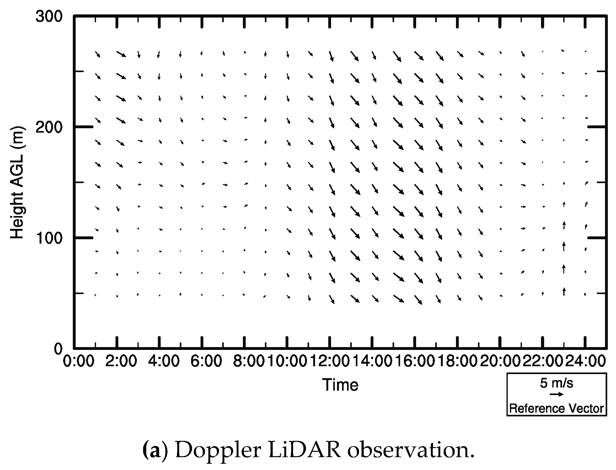

Figure 5.
Vertical wind profiles from Doppler LiDAR observations and from simulations with NLNI-76 and NLNI-09, and potential temperature profiles from simulations with NLNI-76 and NLNI-09, on 11 September 2015: (a) At 08:00, before the sea breeze blows into the Ohashi Doppler LiDAR observation site; (b) At 09:00, the simulation with NLNI-76 captured the sea breeze, while the Doppler LiDAR did not; (c) At 10:00, the Doppler LiDAR captured the sea breeze; (d) At 14:00, the simulation with NLNI-76 showed a potential temperature drop below 50 m above ground level (AGL); (e) At 15:00, the observed sea breeze became the strongest on that day; and (f) At 18:00, the potential temperature profile difference showed a large difference between NLNI-76 and NLNI-09 below 100 m AGL.


Table 1.
Land-use categories in the Weather Research and Forecasting model (WRF) and National Land Numerical Information (NLNI) land-use datasets.
Table 1.
Land-use categories in the Weather Research and Forecasting model (WRF) and National Land Numerical Information (NLNI) land-use datasets.
| Land-Use Categories in WRF (Provided by the U.S. Geological Survey) | Land-Use Categories in NLNI in 1976 | Land-Use Categories in NLNI in 2009 |
|---|---|---|
| Irrigated Cropland and Pasture | Paddy field | Paddy field |
| Mixed Dryland/Irrigated Cropland and Pasture | Field | Other agricultural land |
| Orchard | ||
| Other tree plantation | ||
| Mixed Forest | Forest | Forest |
| Barren or Sparsely Vegetated | Wasteland | Wasteland |
| Other land | Other land | |
| Golf course | ||
| Urban and Built-Up Land | Land for building | Land for building |
| Trunk transportation land | Trunk transportation land (Road) | |
| Trunk transportation land (Rail) | ||
| Water Bodies | Lake | River basin, lake, and marsh |
| River | ||
| Beach | Beach | |
| Seawater body | Seawater body |
Table 2.
Mean error (ME) and root mean square error (RMSE) for the surface air temperature when comparing the JMA observations and the simulation results for NLNI-09 and USGS.
Table 2.
Mean error (ME) and root mean square error (RMSE) for the surface air temperature when comparing the JMA observations and the simulation results for NLNI-09 and USGS.
| Site | NLNI-09 | USGS | ||
|---|---|---|---|---|
| ME (°C) | RMSE (°C) | ME (°C) | RMSE (°C) | |
| 1. Munakata | −0.741 | 2.553 | −1.722 | 3.170 |
| 2. Yahata | 0.633 | 3.150 | −1.038 | 3.324 |
| 3. Kuko-kitamachi | 0.093 | 3.036 | −0.044 | 2.979 |
| 4. Yukuhashi | −0.492 | 3.160 | −1.608 | 3.590 |
| 5. Iizuka | −0.172 | 3.164 | −1.628 | 3.748 |
| 6. Maebaru | 0.052 | 3.191 | −0.998 | 3.296 |
| 7. Fukuoka | 1.430 | 3.397 | 0.674 | 3.081 |
| 8. Hakata | 1.032 | 3.317 | −1.066 | 3.652 |
| 9. Dazaifu | 0.290 | 3.184 | −0.996 | 3.377 |
| 10. Soeda | −1.238 | 3.435 | −0.153 | 3.006 |
| 11. Asakura | −0.208 | 3.473 | −1.193 | 3.708 |
| 12. Kurume | 0.845 | 3.427 | −0.626 | 3.548 |
| 13. Kurogi | −0.665 | 3.435 | −0.904 | 3.466 |
| 14. Omuta | 0.924 | 3.407 | 1.060 | 3.408 |
| Total | 0.128 | 3.247 | −0.731 | 3.391 |
Table 3.
Land-use fractions in the NLNI-09 case, and the dominant land-use category in the USGS case, for the 14 grid cells with a resolution of 1 km that include the JMA observation sites. For the NLNI-09 case, the dominant land-use category is shaded.
Table 3.
Land-use fractions in the NLNI-09 case, and the dominant land-use category in the USGS case, for the 14 grid cells with a resolution of 1 km that include the JMA observation sites. For the NLNI-09 case, the dominant land-use category is shaded.
| Land-Use Fraction in NLNI-09 | Dominant Land-Use Category in USGS | ||||||
|---|---|---|---|---|---|---|---|
| Urban and Built-Up Land | Irrigated Cropland and Pasture | Mixed Dryland/Irrigated Cropland and Pasture | Mixed Forest | Barren or Sparsely Vegetated | Water Bodies | ||
| 1. Munakata | 26.7% | 41.9% | 4.2% | 18.8% | 1.7% | 6.7% | Shrubland |
| 2. Yahata | 67.2% | 0.0% | 0.0% | 12.4% | 20.4% | 0.0% | Cropland/Grassland Mosaic |
| 3. Kuko-kitamachi | 0.1% | 0.0% | 0.0% | 0.0% | 21.3% | 78.5% | Water Bodies |
| 4. Yukuhashi | 50.7% | 39.8% | 1.0% | 0.3% | 3.3% | 4.9% | Cropland/Grassland Mosaic |
| 5. Iizuka | 53.7% | 7.0% | 0.0% | 17.1% | 8.8% | 13.5% | Shrubland |
| 6. Maebaru | 45.0% | 44.5% | 2.0% | 0.0% | 2.5% | 6.0% | Dryland Cropland and Pasture |
| 7. Fukuoka | 74.6% | 0.0% | 0.0% | 8.7% | 8.3% | 8.4% | Urban and Built-up Land |
| 8. Hakata | 46.2% | 0.0% | 0.0% | 6.8% | 45.9% | 1.1% | Shrubland |
| 9. Dazaifu | 57.1% | 5.4% | 9.4% | 18.7% | 8.1% | 1.3% | Shrubland |
| 10. Soeda | 10.4% | 13.8% | 5.2% | 62.3% | 4.8% | 3.5% | Urban and Built-up Land |
| 11. Asakura | 28.6% | 62.1% | 7.2% | 1.7% | 0.4% | 0.0% | Irrigated Cropland and Pasture |
| 12. Kurume | 44.5% | 44.0% | 0.9% | 0.0% | 7.4% | 3.2% | Irrigated Cropland and Pasture |
| 13. Kurogi | 3.3% | 34.2% | 48.0% | 13.0% | 0.0% | 1.5% | Cropland/Woodland Mosaic |
| 14. Omuta | 60.3% | 11.2% | 8.2% | 16.3% | 3.5% | 0.5% | Urban and Built-up Land |
© 2017 by the author. Licensee MDPI, Basel, Switzerland. This article is an open access article distributed under the terms and conditions of the Creative Commons Attribution (CC BY) license (http://creativecommons.org/licenses/by/4.0/).
Share and Cite
MDPI and ACS Style
Kawamoto, Y. Effect of Land-Use Change on the Urban Heat Island in the Fukuoka–Kitakyushu Metropolitan Area, Japan. Sustainability 2017, 9, 1521. https://doi.org/10.3390/su9091521
AMA Style
Kawamoto Y. Effect of Land-Use Change on the Urban Heat Island in the Fukuoka–Kitakyushu Metropolitan Area, Japan. Sustainability. 2017; 9(9):1521. https://doi.org/10.3390/su9091521
Chicago/Turabian StyleKawamoto, Yoichi. 2017. "Effect of Land-Use Change on the Urban Heat Island in the Fukuoka–Kitakyushu Metropolitan Area, Japan" Sustainability 9, no. 9: 1521. https://doi.org/10.3390/su9091521
Note that from the first issue of 2016, this journal uses article numbers instead of page numbers. See further details here.