Uncertainty Analysis of a GHG Emission Model Output Using the Block Bootstrap and Monte Carlo Simulation
by
 , , , ,
Min Hyeok LEE
1 ,
,
Jong Seok LEE
1,
Joo Young LEE
1,
Yoon Ha KIM
1,
Yoo Sung PARK
2 and
Kun Mo LEE
1,* 1
Department of Environmental and Safety Engineering, Eco-Product Research Institute, Ajou University, 206 Worldcup-ro, Yeongtong-gu, Suwon 16499, Korea
2
H.I.Pathway Co., Ltd., 10F #1006, ACE High-End Tower 10th, 30, Gasan Digital 1-ro, Geumcheon-gu, Seoul 08591, Korea
*
Author to whom correspondence should be addressed.
Sustainability 2017, 9(9), 1522; https://doi.org/10.3390/su9091522
Submission received: 27 July 2017
/
Revised: 18 August 2017
/
Accepted: 23 August 2017
/
Published: 26 August 2017
Abstract
:Uncertainty analysis of greenhouse gas (GHG) emissions is becoming increasingly necessary in order to obtain a more accurate estimation of their quantities. The Monte Carlo simulation (MCS) and non-parametric block bootstrap (BB) methods were tested to estimate the uncertainty of GHG emissions from the consumption of feedstuffs and energy by dairy cows. In addition, the contribution to variance (CTV) approach was used to identify significant input variables for the uncertainty analysis. The results demonstrated that the application of the non-parametric BB method to the uncertainty analysis, provides a narrower confidence interval (CI) width, with a smaller percentage uncertainty (U) value of the GHG emission model compared to the MCS method. The CTV approach can reduce the number of input variables needed to collect the expanded number of data points. Future studies can expand on these results by treating the emission factors (EFs) as random variables.
1. Introduction
Recently, interest in greenhouse gas (GHG) emissions from the dairy sector has been increasing because GHG emissions from this sector are estimated to represent 3%–5% of the global GHG emissions [1]. All the industry sectors and individual companies in the field of energy, industrial production, agriculture, and wastes in Korea are required to report their GHG emissions to the legal authorities [2]. Furthermore, Korea began carbon trading in 2015 [3]. Hence, a more accurate quantification of GHG emissions is required.
Uncertainty analysis estimates the amount of deviation in the calculated output of a mathematical model from its true mean. The results of the uncertainty analysis are often expressed as a confidence interval (CI) at a given confidence level. Quite often, the inputs of the model include observation and/or measurement errors, which reduce confidence in the model output [4]. In addition to the measurement error leading to parameter uncertainty of the model output, there are other forms of uncertainty, including scenario and model uncertainty. Scenario uncertainty includes choices regarding functional unit, valuation and weighting factors, time horizons, geographical scales, natural contexts, allocation procedures, waste-handling scenarios, use of environmental thresholds and expected technology trends [5]. Model uncertainty includes models for deriving emissions and characterization factors [5]. In this study, we focused only on parameter uncertainty.
The Intergovernmental Panel on Climate Change (IPCC) provides good practice guidance on a variety of uncertainty analysis methods [6]. The methods advocated by the IPCC are listed under Approaches I and II. Approach I refers to the error propagation (EP) method, and Approach II refers to the Monte Carlo simulation (MCS) method.
The EP method used in IPCC’s Approach I does not consider covariance in the variance calculation. However, the MCS method in IPCC’s Approach II considers covariance. Furthermore, Approach II discusses issues of dependence and correlation [6]. This study considers covariance in all uncertainty analysis methods.
Most of the literature that deals with quantifying GHG emissions in the dairy sector has used the MCS method for uncertainty analysis [7,8,9]. These studies have assumed that all input variables follow parametric distributions, including lognormal and/or normal distributions. Although the MCS method is the method of choice for quantifying uncertainty in the dairy sector, its use for uncertainty analysis has limitations. It requires defining the probability distribution of each input variable, which might be more difficult if empirical information is unavailable [8]. Basset-Mens et al. [7] highlighted the difficulties in defining probability distribution for input variables in the life cycle assessment (LCA) studies. Therefore, when the probability distribution of the data points of the input variable is uncertain, other uncertainty methods or probability distributions should be considered, instead of parametric distribution, for analyzing the uncertainty of GHG emissions in the dairy sector.
Because any mathematical model consists of many input variables, an efficient method should be developed to identify the input variables that contribute considerably to the uncertainty of the model output. Global sensitivity analysis or contribution to variance (CTV) approach is an effective tool for this purpose [10,11,12]. The input variables identified as significant to the process become targets for further scrutiny. The results of the sensitivity analysis enable focusing on the identified input variables, such that their observation/measurement errors can be reduced through the use of a larger number of data points. Therefore, the use of the CTV approach simplifies the mathematical model by removing insignificant input variables from the model.
The objective of this study was to compare uncertainty analysis methods for the quantification of uncertainties in the output of the GHG emission model. A linear GHG emission model was formulated to assess the environmental impact of GHG emissions generated at a dairy cow farm in Korea. Two different methods, the MCS and non-parametric block bootstrap (BB), were used to analyze the uncertainty of the GHG emissions model output.
2. Methods
2.1. Greenhouse Gas Emission Model
The GHG emissions model has two major components: activity data and emission factors (EFs). Activity data include data related to materials and energy consumed in a production system, which can be readily collected from the site. EFs, however, are difficult to obtain, because limited studies in the literature have estimated them. Therefore, the EF was assumed to be a constant in the GHG emission model. In addition, the GHG emission model was chosen to be linear, as shown in Equation (1). The input variables were collected and substituted into Equation (1) to calculate the model output.
where is the GHG emissions model output (kg CO2-eq/(head-month)); is the column vector of ; is the GHG EF (kg CO2-eq/kg or kWh) of the ith substance (feedstuff and energy in this study); is the vector of ; is the average of , and is the mass and energy of the ith substance (kg or kWh/head-month). Head-month denotes one head of cow during a month.
2.2. Error Propagation Equation Method
Equation (2) is a generic equation for the quantification of the variance of the model output () as a function of the variances of the input variables and their EFs in the form of a matrix [13]. In most life cycle impact assessment (LCIA) studies, covariance is often assumed to be negligible [14]. However, this assumption cannot be substantiated unless the independence of the input variables is ensured.
where is the variance of z, is the transpose of , and V is the variance-covariance matrix of the input variables .
2.3. Identification of Xi That Contributes Considerably to
As the name suggests, contribution analysis is conducted to identify input variables that contribute considerably to the model output by estimating their relative contribution [15]. However, contribution analysis does not consider the variances of the input variables with respect to the uncertainty of the model output. Therefore, it is not an appropriate method for analytical error analysis. Thus, identification of significant input variables requiring a larger number of data points, using CTV analysis based on the error propagation (EP) method, is a logical choice for uncertainty analysis.
The variance and mean of Z are calculated to estimate the uncertainty of the model output. CTV is often used to evaluate the degree of dispersion of the data of a random variable and the output of a model [11,16]. Thus, Equation (3) is used for identifying the input variables that significantly contribute to the variance of the model output. This value represents the degree of contribution of the input variable to the variance of the model output () [10]. The input variables exhibiting high CTV do require additional data points. The variance of the model output is then calculated using additional data points.
2.4. Monte Carlo Simulation Method
The MCS method estimates the uncertainty of the model output by randomly generating data points of each input variable, based on the probability distribution of the input variable, and feedings them into the GHG emission model in Equation (1) [17].
A parametric distribution is defined as the one using mathematics for describing the probability model [18,19]. Meanwhile, a non-parametric (or empirical) distribution is based on the observed data of the input variable. Parameters were initially selected for a variety of distributions. Subsequently, the parameter values of the distribution were calculated using the maximum likelihood estimation method [20]. The parametric probability distribution and its parameter values for the input variables of the MCS method were estimated using the Anderson–Darling (AD) test, which is a goodness-of-fit test. The p-value and AD statistic were used to test the null hypothesis for the assumed probability distributions of the input variable. The probability distribution with the smallest AD statistic among the assumed probability distributions, with a p-value greater than 0.05, was chosen as the probability distribution of the input variable. The estimated parametric probability distribution and its parameter values were used for implementing MCS.
The non-parametric probability distribution and its parameter values of the input variables for the MCS method were estimated using the histogram approach. In order to create a histogram, the number of bins (k) and the width of the bins (h) of the input variables were calculated as shown in Equation (4).
where x is the value of the input variable X, k is the number of bins; h is the width of bins.
The number of bins, k, was calculated using Doane’s formula [21]. Based on the values of k and h, the probability of data points of the input variable in each bin was obtained. This information was subsequently used for implementing MCS.
Thus, two combinations of the probability distributions of input variables were estimated for the MCS method: parametric and non-parametric. The estimated probability distributions of the input variables with relevant parameter values were fed into the MCS software. In addition, this study considered dependence of the input variables in the MCS method by applying the Spearman rank order correlation coefficient.
The probability distribution of the model output was obtained by repeating the procedure several times (in this study, n = 10,000). Subsequently, the mean, variance, and CI of the model output were computed. The CI of the model output from the MCS method was obtained using the percentile approach, where upper and lower bounds of the 95% CI were 0.025 and 0.975 quantile of the model outputs, respectively.
2.5. Block Bootstrap Method
The bootstrap method considers the data collected to be the original sample. Then, random sampling of the original data with the replacement creates a sample, where the number of elements is the same as the original sample, while the data differ from the original. By repeating the resampling process several times with replacements, a large number of resampled data sets are created [22]. Further, Xi are not independent, because the covariance of the V matrix is not zero [23]. Therefore, the BB method was chosen to reflect the dependency among the input variables.
A simple example of the BB method is given below. Let us consider that random variables X and Y have values of x = (1, 2, 3) and y = (8, 12, 16). The covariance of X and Y is 4, and its correlation coefficient is 1. Therefore, X and Y have positive dependence. The bootstrap method performs the resampling of X and Y separately, such that the dependence between the two random variables cannot be maintained. For the resampled X and Y, shown in Table 1, the covariance and correlation coefficients of the first and second replicates differ. However, the BB method creates a block using paired data, for example, (xi, yi), subsequently generating replicates through resampling. The covariance of the original sample and the BB’s first and second replicates are positive. The correlation coefficients of the original sample are the same as those of the resampled replicates. As such, the positive dependence between X and Y remains intact.
The independent and identically distributed bootstrap method fails drastically when using dependent data. Therefore, a more general resampling scheme, which is applicable without any parametric model assumption, such as BB, can be used [24].
The non-parametric BB method was applied to analyze a GHG emission model output that does not require estimating the probability distribution of the input variable. In this study, a total of 11 in a given month were treated as a block, with n blocks in the matrix of the input variables. The EF of an input variable was applied to the variable to generate GHG emissions from it. The column mean of GHG emissions under each input variable was calculated from the column sum, with these column means being added to obtain the model output). This exercise was repeated 1000 times (i.e., R = 1000).
Thus, there were a total of 1000 GHG emission model output values, from . Equation (5) shows the percentile approach, where 95% CI of the GHG emission output can be obtained.
where is the original GHG emission model output, is the BB resampled GHG emission model output (1000 samples), and is the difference between and [22].
2.6. Statistics for Assessing the Uncertainty of the Model Output
Two statistics were used to assess the accuracy of the estimated mean of the GHG emission model output: CI and percentage uncertainty (U). The CI of the model output was estimated at the 95% confidence level. The 95% CI indicates that the true mean of the population lies between the upper and lower bounds of the CI 95 times out of 100 samplings. U is a statistic used in the IPCC guide as a measure of the uncertainty of the model output. U is defined as the ratio of the half-width of the 95% CI of the model output to the mean of the model output [6]. A narrower CI and a smaller U value reflect a more precise estimate of the mean of the model output. In other words, the narrower the CI and smaller the U value indicate more accurate the GHG emission model output.
2.7. Data Collection
A dairy cow farm located in Hwasung-si, western part of Korea, was the target farm for data collection. The farm has a total of 88 Holstein cows in an area of 3041 m2. Most dairy cow farms in Korea have 50 to 100 Holstein cows, making the target farm we worked on a typical dairy cow farm in Korea.
The farmer recorded the actual amounts of feedstuff fed to the dairy cows and the energy consumed to maintain the farm on a monthly basis. The collected monthly data were normalized according to the total number of cows. The type of feed or feedstuff, such as feed for dry cows, feed for lactating cows, alfalfa, straw, oats, corn silage, rapeseed, bagasse, and soybean meal, and the source of energy used, such as electricity and diesel, represent the input variables (). The farmer had already recorded the data associated with some of the input variables for six years. These data were used to assess the effect of the expanded number of data on reducing uncertainty.
3. Results and Discussion
Data from a dairy cow farm located in Korea were used in the case study to compare the two above-mentioned uncertainty analysis methods [25]. The number of heads in the dairy cow farm was used to normalize the collected data. Table 2 shows the normalized initial data, mean, standard deviation (SD), and GHG EF [26] of the input variables.
A total of 72 monthly data for the input variables were collected. Initially, the most recent 1-year data of the 12-monthly data were used in the uncertainty analysis. Once significant input variables were identified using the 12 data of each of the 11 input variables, the data for 6 years, totaling 72 monthly data of the identified input variables, were used.
The relative errors of the input variables, which is the ratio of the SD divided by the mean, ranged from 31% to 81%, with a simple average of 54%. This indicates that the data variability was not high, being approximately 0.5.
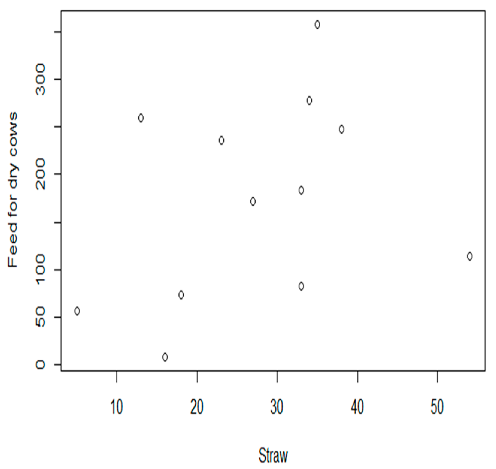
Figure 1 shows the scatter plot of the comparison between feed for dry cows and straw. A correlation was observed between the two variables. Furthermore, a similar trend can be observed among all the input variables. In addition, the covariance between the input variables is not zero, which indicates that there is some degree of association between the input variables. In other words, nonzero covariance implies that the returns of two input variables share some degree of correlation [27].
The correlation test results for the significant input variables are shown in Table 3. The results show that there are dependencies among the significant input variables.
The probability distribution of the input variables was evaluated [28]. The hypotheses for testing the probability distribution using the AD test were as follows. H0: the input data follow a specified distribution, H1: the input data do not follow a specified distribution. According to the hypothesis testing of normality, 7 input variables (feed for dry cows, alfalfa, straw, corn silage, rapeseed, bagasse, and electricity) out of 11 showed p-values greater than the significance level (, which indicates that they may follow a normal distribution. On the other hand, the probability distribution of the remaining variables showed that three of them (feed for lactating cows, oats, and diesel) may follow a lognormal distribution, with the last one (soybean meal) following a logistic distribution.
Table 4 shows the estimated parametric probability distribution of the input variables with 12 and 72 monthly data points for the MCS method. Dependence among the input variables was taken into consideration by applying the Spearman rank order correlation coefficient in the case of the MCS method. Spearman rank order correlation coefficients were applied to the paired input variables using Oracle Crystal ball software [29]. Fifty-five correlation coefficients were applied for 11 input variables, whereas 15 correlation coefficients were applied for 6 input variables. Non-parametric probability distributions of the input variables were estimated by using the histogram with data.
In addition, normality plotting (Q–Q plotting) was performed to evaluate the normality of the input variables. However, this plot requires subjective judgment. In the case of seven variables, no conclusive fit could be found to ascertain that they follow a normal distribution. Although the normality test of the input variables using both, the hypothesis test and normality plot, produced positive results, these do not necessarily guarantee normal distribution of the variables. Therefore, there is some uncertainty about the true probability distribution of the input variables.
Covariance is also an important statistic in estimating uncertainty. However, EFs were not treated as random variables in this study. Therefore, only covariance of the input variables was considered in the uncertainty analysis.
Table 5 shows the results of the uncertainty analysis of the GHG emission model for the MCS (with the parametric and non-parametric probability distributions) and BB methods when the number of data points for each input variable is 12.
Table 5 shows that the BB method provides the narrowest CI width and the smallest U value, followed by the non-parametric probability distribution, and parametric probability distribution of the MCS method. The CI width and the U value of the non-parametric probability distribution were approximately 54% and 63% of those of the parametric probability distribution of the MCS method, respectively. Meanwhile, the CI width and the U value of the BB method were 36% and 33% of the CI width of the non-parametric probability distribution of the MCS method, respectively.
Table 6 shows the results of the two uncertainty analysis methods based on the expanded number of data points for the six input variables (n = 72).
The same trend can be observed in the case of n = 72. This shows that all the statistical values of the expanded number of data points (n = 72) decreased compared to those of the initial number of data points (n = 12). In the case of the BB method, for instance, the percent reduction in the CI width and U value going from n = 12 to n = 72 were 80% and 77%, respectively.
Table 5 and Table 6 show that the size of CI and the value of U decreases in order, from the parametric MCS to non-parametric MCS method to the BB method. The same trend can be observed with regard to uncertainty of water scarcity footprint (WSF) of a water purifier and rice production in a drainage basin in Korea [30].
The WSF was calculated using 42 annual data of water resources and water consumption, while the value of U was calculated using the parametric and non-parametric MCS methods, as well as BB method. The value of U with regard to the water purifier using the parametric and non-parametric MCS and BB methods were 118.4%, 103.7%, and 18.9%, respectively [30]. With regard to rice production, they were 146.0%, 103.0%, and 19.0%, respectively [30]. There was a significant drop in the value of U and CI from the MCS method to the BB method, although the difference between the parametric and non-parametric MCS was not large.
Decrease in the value of U and CI from the MCS method to the BB method may be due to errors in estimating parametric and non-parametric probability distribution of the input variables for the MCS method. Although non-parametric distribution generates a lower estimate of uncertainty compared to parametric distribution, the difference is minor, which cannot be the basis for claiming that non-parametric probability distribution is preferred over parametric probability distribution in the MCS method. This is mainly because this study is based on a single system with a relatively small number of data points.
Several studies on uncertainty analysis using the MCS method in the LCIA field assumed probability distributions or relied on the judgment of an expert [7,8,31]. Assumed parametric probability distribution or ignoring the covariance of the input variables, would lead to poorer estimation of the variance of the model output, leading to a less accurate estimate of the uncertainty of the model output.
It is premature to conclude that the BB method produces narrower CI and smaller value of U compared to the MCS method in every system. However, this study and the WSF study [30] showed that the BB method produces a lower estimate of uncertainty compared to the parametric and non-parametric distribution MCS method, most likely due to its distribution-free nature.
The BB method requires many repeated data points of the input variables for resampling. In LCA, we rarely have the ability to measure all input variables repeatedly. Therefore, this is one of the limitations of the BB method. Meanwhile, the parametric MCS method requires probability distribution of the input variable and its parameter values. However, they are often difficult to estimate with accuracy. The non-parametric MCS method requires empirical distribution using methods such as histogram. However, this requires a large number of data points of the input variable. In this study, we have only 12 to 72 data points of the input variable, causing the non-parametric distribution estimated from the use of histogram to be potentially inaccurate.
The parametric cumulative distribution (CDF) plot of diesel, shown in Figure 2, exhibits that there is a 3% probability of exceeding the maximum observed value of 22 kg/head-month when the sample size is small (n = 12). When the sample size is large (n = 72), the probability of exceeding the maximum observed value is 0%. The same is true in case of feed for lactating cows.
These results are in agreement with the theory that a parametric fit could better capture the potential for long tails in the probability density functions (pdfs). With regard to the parametric CDF of feed for lactating cows, when n = 12, there is a 10% probability of exceeding the maximum observed value of 786 kg/head-month. However, the parametric CDF predicts a non-zero probability of exceeding 1300 kg/head-month. Normally, a cow farm does not feed the cows this amount. Therefore, this value is considered unrealistic. Thus, parametric probability distribution may produce an erroneous model output, since its pdf includes an unrealistic input value. Meanwhile, non-parametric probability distribution is formulated empirically, based on actual data, preventing the input of an erroneous value.
Table 7 shows the variance of the GHG emission model output, with and without considering the covariance for n = 12 and 72. The variance was calculated using the EP method.
Since the EP method does not generate a CI, the CI width and U value cannot be computed. This makes the EP method less desirable for uncertainty analysis. The EP method is used to calculate the variance of the model output analytically, which can be used to compare with the variances from the MCS and BB methods.
The variance of the GHG model calculated using the EP method shown in Table 7 was 34,013, by considering covariance (it was 19,726 without considering covariance) when n = 12. The variance of the model output from the BB and non-parametric probability distribution of the MCS methods, when n = 12, were 31,053 and 25,730, respectively. These three variance values are similar to each other. Meanwhile, the variance with the parametric probability distribution of the MCS method when n = 12 was 100,827, which is approximately three times greater than those of the other three results. The same trend can be observed when n = 72. Thus, the parametric probability distribution method appears to overestimate the variance of the GHG model output.
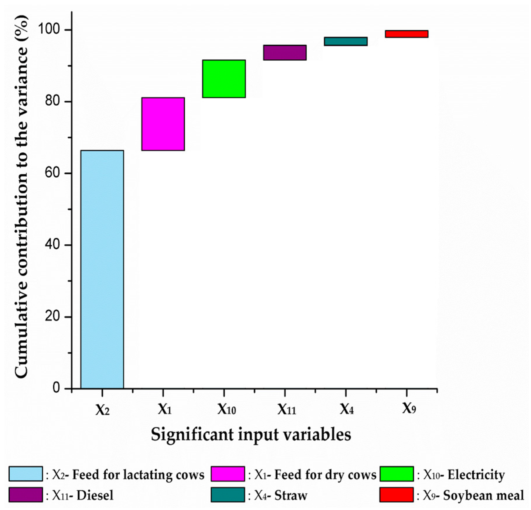
The EP method can be used for the CTV analysis to identify the input variables that contribute considerably to the total variance of the model output. Figure 3 shows the cumulative contribution of the 6 input variables based on the initial data of 11 input variables, namely 99.8% of the total variance. The variance of the feed for lactating cows contributed the most, followed by the feed for dry cows, electricity, diesel, straw, and soybean meal. Therefore, these six variables were selected as the targets for the expanded data collection, with n = 72. On the other hand, the contributions of the remaining five variables to the variance of the model output were considered negligible.
It is well-known that a higher number of data points reduces the variance of the mean, also lowering the uncertainty of the model output. The finding in this study is that the CTV approach can minimize the number of input variables for collecting an expanded number of data points. For example, in this study, if the input variables would be limited to those contributing at least 95% to the model output variance, the number of input variables for the expanded data collection would be reduced to four (feed for lactating cows, feed for dry cows, electricity, and diesel).
Both, the activity data and the EFs, influence the uncertainty of the model output in LCIA [7,8,31]. However, this study did not treat the EFs as random variables, which is its limitation. The reason for treating EFs as a constant was that the EFs derived from the Korean LCA database have many shortcomings from a statistical standpoint (e.g., fewer studies, limited number of data points, less transparent system boundaries of the LCA studies, etc.).
When EF is treated as a random variable in addition to the current input variable in this study, the GHG emission model contains two independent random variables. In this case, the bootstrapping method can be applied by resampling both variables separately, subsequently taking the average of the resampled data of each variable and multiplying the two averages to generate the GHG emission value. By repeating this procedure, say, 1000 times, the average GHG emission values are used to produce 95% CI of the GHG emissions using the percentile method.
4. Conclusions
The major conclusions of this study are as follows.
The EP method is used to calculate the variance of the model output analytically. The variance thus calculated can be used for comparison with the variances from the MCS and BB methods. In addition, the EP method can be used for the CTV analysis.
This study showed that the BB method produces a lower estimate of uncertainty compared to the parametric and non-parametric distribution MCS methods, most likely due to its distribution-free nature. However, it is premature to conclude that the BB method produces a narrower CI and smaller value of U compared to the parametric and non-parametric probability distribution MCS methods in every system. This is because this study is based on only one system, with a limited number of data points.
The CTV approach can reduce the number of input variables for collecting the expanded number of data points. It should also be noted that this study suffers from a shortcoming, namely, the EFs were not treated as random variables. Future studies should treat the EFs as random variables, to properly reflect their contributions to the uncertainty of model output.
Acknowledgments
This study was supported by the “Cooperative Research Program for Agriculture Science & Technology Development” of the Korea Rural Development Administration (Project No. PJ011762022017).
Author Contributions
Min Hyeok Lee conducted the research with the help from Yoo Sung Park. Both authors collected data and analyzed the uncertainty of the model output. Jong Seok Lee, Joo Young Lee and Yoon Ha Kim conducted the R programming of the uncertainty analysis methods. Kun Mo Lee conceived the research idea, providing details of the uncertainty analysis methods, while supervising the entire research process.
Conflicts of Interest
The authors declare no conflicts of interest.
References
- FAO (Faostat). Greenhouse Gas Emissions from the Dairy Sector; Food and Agriculture Organization of the United Nations: Rome, Italy, 2010. [Google Scholar]
- MOE. The Framework Act on Low Carbon, Green Growth; Korean Ministry of Environment: Sejong City, Korea, 2013.
- MOE. The Act on the Allocation and Trading of Greenhouse Gas Emission Permits; Korean Ministry of Environment: Sejong City, Korea, 2012.
- Der Kiureghian, A.; Ditlevsen, O. Aleatory or epistemic? Does it matter? Struct. Saf. 2009, 31, 105–112. [Google Scholar] [CrossRef]
- Lloyd, S.M.; Ries, R. Characterizing, Propagating, and Analyzing Uncertainty in Life-Cycle Assessment. J. Ind. Ecol. 2007, 11, 161–179. [Google Scholar] [CrossRef]
- Intergovernmental Panel on Climate Change (IPCC). Guidelines for National Greenhouse Gas Inventories Chapter 3 of Volume 1; Intergovernmental Panel ON Climate Change (IPCC): Hayama, Japan, 2006. [Google Scholar]
- Basset-Mens, C.; Kelliher, F.M.; Ledgard, S.; Cox, N. Uncertainty of global warming potential for milk production on a New Zealand farm and implications for decision making. Int. J. Life Cycle Assess. 2009, 14, 630–638. [Google Scholar] [CrossRef]
- Chen, X.; Corson, M.S. Influence of emission-factor uncertainty and farm-characteristic variability in LCA estimates of environmental impacts of French dairy farms. J. Clean. Prod. 2014, 81, 150–157. [Google Scholar] [CrossRef]
- Flysjö, A.; Henriksson, M.; Cederberg, C.; Ledgard, S.; Englund, J.-E. The impact of various parameters on the carbon footprint of milk production in New Zealand and Sweden. Agric. Syst. 2011, 104, 459–469. [Google Scholar] [CrossRef]
- Heijungs, R.; Lenzen, M. Error propagation methods for lca—A comparison. Int. J. Life Cycle Assess. 2014, 19, 1445–1461. [Google Scholar] [CrossRef]
- Saltelli, A.; Ratto, M.; Andres, T.; Campolongo, F.; Cariboni, J.; Gatelli, D.; Saisana, M.; Tarantola, S. Global Sensitivity Analysis: The Primer; John Wiley & Sons: Hoboken, NJ, USA, 2008; pp. 157–158. [Google Scholar]
- Wolf, P.; Groen, E.A.; Berg, W.; Prochnow, A.; Bokkers, E.A.; Heijungs, R.; de Boer, I.J. Assessing greenhouse gas emissions of milk production: Which parameters are essential? Int. J. Life Cycle Assess. 2017, 22, 441–455. [Google Scholar] [CrossRef]
- Tellinghuisen, J. Statistical error propagation. J. Phys. Chem. A. 2001, 105, 3917–3921. [Google Scholar] [CrossRef]
- Heijungs, R. Sensitivity coefficients for matrix-based lca. Int. J. Life Cycle Assess. 2010, 15, 511–520. [Google Scholar] [CrossRef]
- International Organization for Standardization (ISO). ISO 14044:2006. Environmental Management—Life Cycle Assessment—Requirements and Guidelines; ISO: Geneva, Switzerland, 2006. [Google Scholar]
- Saltelli, A. Global sensitivity analysis: An introduction. In Proceedings of the 4th International Conference on Sensitivity Analysis of Model Output (SAMO’04), Santa Fe, NM, USA, 8–11 March 2004; pp. 27–43. [Google Scholar]
- Bevington, P.R.; Robinson, D.K. Data Reduction and Error Analysis; McGraw-Hill: New York, NY, USA, 2003; pp. 36–50. [Google Scholar]
- Vose Software Homepage. Non-Parametric and Parametric Distributions. Available online: http://www.vosesoftware.com/riskwiki/Parametricandnon-parametricdistributions.php (accessed on 17 July 2017).
- ModelAssist for Risk® Homepage. Non-Parametric and Parametric Distributions. Available online: http://www.epixanalytics.com/modelassist/AtRisk/Model_Assist.htm#Modeling_expert_opinions/Non-parametric_and_parametric_distributions.htm (accessed on 17 July 2017).
- Minitab®17 Homepage. The Anderson-Darling Statistic. Available online: http://support.minitab.com/en-us/minitab/17/topic-library/basic-statistics-and-graphs/introductory-concepts/data-concepts/anderson-darling/#what-is-the-anderson-darling-statistic (accessed on 17 July 2017).
- Doane, D.P. Aesthetic frequency classifications. Am. Stat. 1976, 30, 181–183. [Google Scholar]
- Davison, A.C.; Hinkley, D.V. Bootstrap Methods and Their Application; Cambridge University Press: Cambridge, UK, 1997; Volume 1, pp. 385–436. [Google Scholar]
- Bertsekas, D.P.; Tsitsiklis, J.N. Introduction to Probability; Athena Scientific Belmont: Belmont, MA, USA, 2002; Volume 1, pp. 217–222. [Google Scholar]
- Lahiri, S.N. Scope of Resampling Methods for Dependent Data. In Resampling Methods for Dependent Data, 1st ed.; Springer: New York, NY, USA, 2003; pp. 1–21. [Google Scholar]
- Baek, C.Y.; Lee, K.M.; Park, K.H. Quantification and control of the greenhouse gas emissions from a dairy cow system. J. Clean. Prod. 2014, 70, 50–60. [Google Scholar] [CrossRef]
- Lee, K.M.; Park, K.H. Development of Carbon Tracing System for Livestock Agriculture: Development of LCI DB and Estimation of Greenhouse Gas from Feedstuff Research Report; Rural Development Administration: Jeonju, Korea, 2012.
- Vidyamurthy, G. Pairs Trading: Quantitative Methods and Analysis; John Wiley & Sons: Hoboken, NJ, USA, 2004; Volume 217, pp. 37–51. [Google Scholar]
- Minitab® 17.3.1, Computer Software; Minitab, Inc.: State College, PA, USA, 2016.
- Crystal Ball, Classroom Edition 11.1.4100.0; Oracle, Cor.: Redwood Shores, CA, USA, 2014.
- LEE, J.S.; LEE, M.H.; LEE, J.Y.; KIM, Y.H.; LEE, K.M. Uncertainty analysis of the water scarcity footprint based on the AWARE model. Int. J. Life Cycle Assess. 2017. submitted. [Google Scholar]
- Henriksson, M.; Flysjö, A.; Cederberg, C.; Swensson, C. Variation in carbon footprint of milk due to management differences between swedish dairy farms. Animal 2011, 5, 1474–1484. [Google Scholar] [CrossRef] [PubMed]
Figure 1.
Scatter plot between feed for dry cows and straw (unit: kg feed/head-month).

Figure 2.
Cumulative density function of diesel and feed for lactating cows.
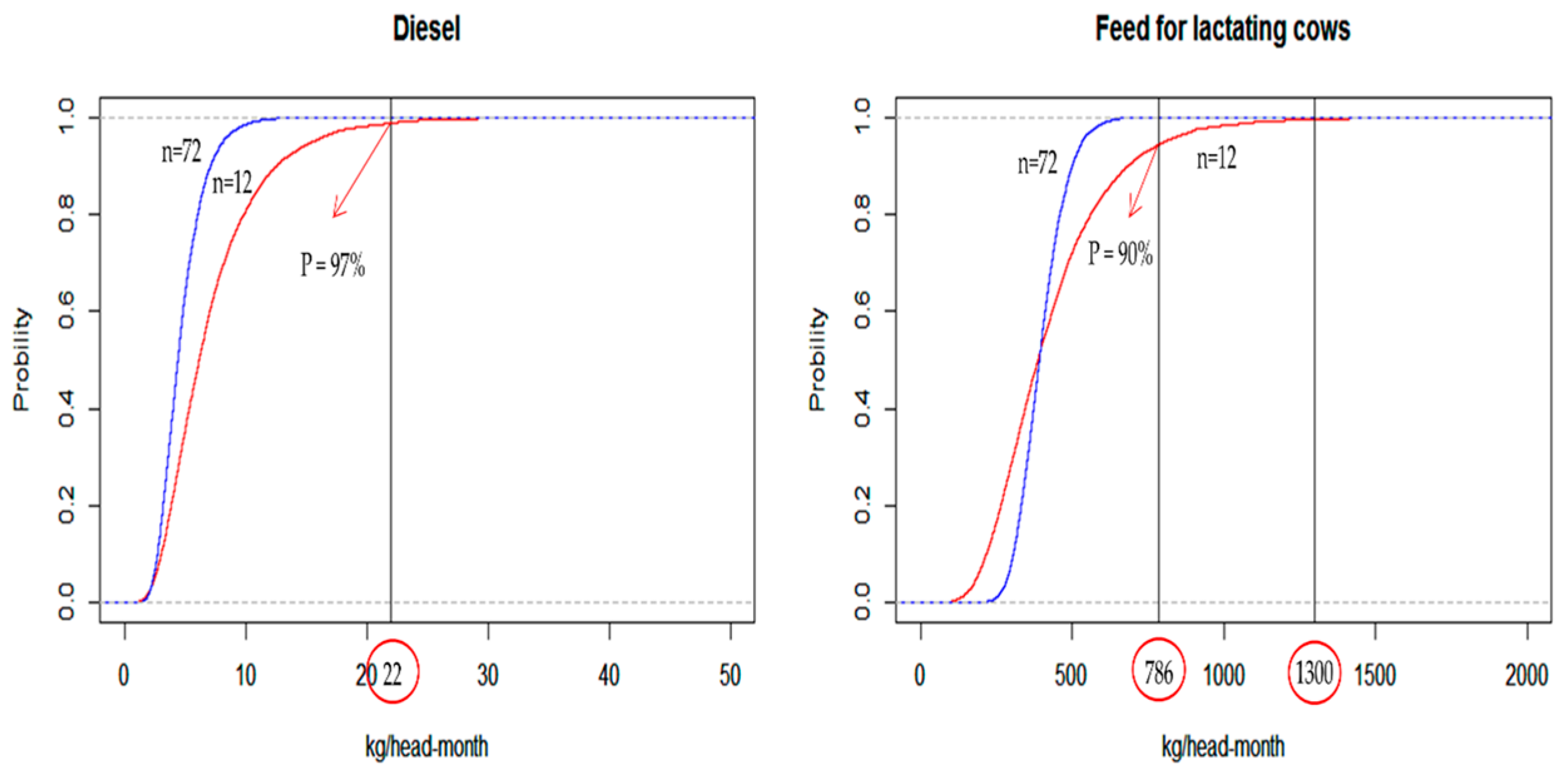
Figure 3.
Cumulative contribution of contribution to variance (CTV) of the significant input variables to the model output.
Figure 3.
Cumulative contribution of contribution to variance (CTV) of the significant input variables to the model output.

Table 1.
Example of the bootstrap and block bootstrap (BB) resampled samples.
| Bootstrap | BB | |||||||
|---|---|---|---|---|---|---|---|---|
| Resampled samples | First Replicate | Second Replicate | First Replicate | Second Replicate | ||||
| X | Y | X | Y | X | Y | X | Y | |
| 3 | 8 | 3 | 12 | 3 | 16 | 3 | 16 | |
| 2 | 12 | 3 | 16 | 2 | 12 | 3 | 16 | |
| 1 | 16 | 1 | 16 | 1 | 8 | 1 | 8 | |
| Covariance | −4.0 | −1.3 | +4.0 | +5.3 | ||||
| Correlation coefficient | −1.0 | −0.5 | 1.0 | 1.0 | ||||
Table 2.
Normalized initial data, mean and standard deviation (SD), and greenhouse gas emission factors (GHG EFs) of the input variables (unit; kg feed/head-month).
Table 2.
Normalized initial data, mean and standard deviation (SD), and greenhouse gas emission factors (GHG EFs) of the input variables (unit; kg feed/head-month).
| Month | Feed for Dry Cows | Feed for Lactating Cows | Alfalfa | Straw | Oats | Corn Silage | Rape Seed | Bagasse | Soybean Meal | Electricity 2 | Diesel 3 |
|---|---|---|---|---|---|---|---|---|---|---|---|
| X1 | X2 | X3 | X4 | X5 | X6 | X7 | X8 | X9 | X10 | X11 | |
| 1 | 114 | 299 | 23 | 54 | 56 | 180 | 15 | 9 | 13 | 161 | 5 |
| 2 | 260 | 411 | 28 | 13 | 59 | 103 | 29 | 19 | 17 | 113 | 5 |
| 3 | 278 | 320 | 30 | 34 | 24 | 94 | 31 | 35 | 18 | 121 | 3 |
| 4 | 236 | 676 | 37 | 23 | 21 | 169 | 27 | 69 | 46 | 160 | 22 |
| 5 | 248 | 741 | 39 | 38 | 8 | 177 | 27 | 13 | 14 | 225 | 5 |
| 6 | 183 | 384 | 28 | 33 | 9 | 320 | 30 | 23 | 16 | 216 | 5 |
| 7 | 358 | 443 | 31 | 35 | 11 | 97 | 21 | 24 | 13 | 109 | 6 |
| 8 | 172 | 786 | 17 | 27 | 10 | 91 | 26 | 4 | 19 | 125 | 10 |
| 9 | 83 | 294 | 34 | 33 | 21 | 161 | 17 | 29 | 14 | 134 | 5 |
| 10 | 73 | 221 | 29 | 18 | 22 | 37 | 22 | 25 | 16 | 27 | 4 |
| 11 | 8 | 241 | 28 | 16 | 18 | 174 | 22 | 12 | 19 | 35 | 5 |
| 12 | 57 | 239 | 8 | 5 | 43 | 83 | 8 | 4 | 4 | 138 | 13 |
| Mean | 172.5 | 421.3 | 27.7 | 27.4 | 25.2 | 140.5 | 22.9 | 22.2 | 17.4 | 130.3 | 7.30 |
| SD | 106.5 | 202.1 | 8.51 | 13.3 | 17.8 | 73.5 | 6.88 | 17.7 | 9.86 | 59.4 | 5.38 |
| Max | 358 | 786 | 39 | 54 | 59 | 320 | 31 | 69 | 46 | 225 | 22 |
| EF 1 | 0.38 | 0.64 | 0.33 | 0.95 | 0.58 | 0.077 | 0.43 | 0.021 | 0.71 | 0.50 | 3.3 |
Notes: 1 Unit: kg CO2-eq/kg; 2 Unit: kWh electricity/head-month; 3 Unit: kg diesel/head-month.
Table 3.
Correlation coefficients for the significant input variables.
| Correlation | Feed for Dry Cows | Feed for Lactating Cows | Straw | Soybean Meal | Electricity | Diesel |
|---|---|---|---|---|---|---|
| Feed for dry cows | 1.0000 | 0.1806 | 0.0610 | 0.0473 | 0.1656 | −0.0099 |
| Feed for lactating cows | 0.1806 | 1.0000 | 0.2244 | 0.3736 | 0.5469 | 0.4177 |
| Straw | 0.0610 | 0.2244 | 1.0000 | 0.0564 | 0.4231 | −0.2554 |
| Soybean meal | 0.0473 | 0.3736 | 0.0564 | 1.0000 | 0.0932 | 0.3885 |
| Electricity | 0.1656 | 0.5469 | 0.4231 | 0.0932 | 1.0000 | 0.2419 |
| Diesel | −0.0099 | 0.4177 | −0.2554 | 0.3885 | 0.2419 | 1.0000 |
Table 4.
Estimated parametric probability distribution of the input variables for the Monte Carlo simulation (MCS) method.
Table 4.
Estimated parametric probability distribution of the input variables for the Monte Carlo simulation (MCS) method.
| Input Variables | Parametric Probability Distribution | |||||
|---|---|---|---|---|---|---|
| n = 12 | Parameters | n = 72 | Parameters | |||
| Location | Scale | Location | Scale | |||
| Feed for dry cows | Normal | 173 | 107 | Lognormal | 208 | 277 |
| Feed for lactating cows | Lognormal | 455 | 433 | Lognormal | 398 | 76.2 |
| Alfalfa * | Normal | 27.6 | 8.66 | - | ||
| Straw | Normal | 27.5 | 13.3 | Lognormal | 29.4 | 6.41 |
| Oat * | Lognormal | 26.0 | 20.0 | - | ||
| Corn silage * | Normal | 141 | 73.5 | - | ||
| Rapeseed * | Normal | 22.9 | 6.89 | - | ||
| Bagasse * | Normal | 22.2 | 17.7 | - | ||
| Soybean meal | Logistic | 16.0 | 3.91 | Logistic | 18.1 | 2.55 |
| Electricity | Normal | 130 | 59.5 | Lognormal | 122 | 25.4 |
| Diesel | Lognormal | 7.00 | 6.00 | Lognormal | 4.71 | 1.78 |
Notes: * The CTV analysis indicated that these input variables were not significant contributors to the variance of the model output.
Table 5.
Uncertainty of the model output based on the two uncertainty analysis methods: n = 12 (unit for z and confidence interval (CI): kg CO2-eq/head-month).
Table 5.
Uncertainty of the model output based on the two uncertainty analysis methods: n = 12 (unit for z and confidence interval (CI): kg CO2-eq/head-month).
| Statistic | MCS | BB | |
|---|---|---|---|
| Parametric | Non-Parametric | ||
| 100,827 | 25,730 | 31,053 | |
| z | 525 | 503 | 505 |
| CI | [265, 1276] | [277, 823] | [405, 605] |
| CI width | 1011 | 546 | 200 |
| U (%) | 96 | 60 | 20 |
Table 6.
Uncertainty of the model output based on the two uncertainty analysis methods: n = 72 (unit for z and CI: kg CO2-eq/head-month).
Table 6.
Uncertainty of the model output based on the two uncertainty analysis methods: n = 72 (unit for z and CI: kg CO2-eq/head-month).
| Statistic | MCS | BB | |
|---|---|---|---|
| Parametric | Non-Parametric | ||
| 17,812 | 6855 | 6554 | |
| z | 450 | 438 | 437 |
| CI | [291, 759] | [300, 690] | [417, 456] |
| CI width | 468 | 390 | 39 |
| U (%) | 52 | 45 | 4.5 |
Table 7.
Variance of the model output.
| Number of Data Points (n) | 12 | 72 |
|---|---|---|
| Without considering covariance | 19,726 | 4665 |
| With considering covariance | 34,013 | 7153 |
© 2017 by the authors. Licensee MDPI, Basel, Switzerland. This article is an open access article distributed under the terms and conditions of the Creative Commons Attribution (CC BY) license (http://creativecommons.org/licenses/by/4.0/).
Share and Cite
MDPI and ACS Style
LEE, M.H.; LEE, J.S.; LEE, J.Y.; KIM, Y.H.; PARK, Y.S.; LEE, K.M. Uncertainty Analysis of a GHG Emission Model Output Using the Block Bootstrap and Monte Carlo Simulation. Sustainability 2017, 9, 1522. https://doi.org/10.3390/su9091522
AMA Style
LEE MH, LEE JS, LEE JY, KIM YH, PARK YS, LEE KM. Uncertainty Analysis of a GHG Emission Model Output Using the Block Bootstrap and Monte Carlo Simulation. Sustainability. 2017; 9(9):1522. https://doi.org/10.3390/su9091522
Chicago/Turabian StyleLEE, Min Hyeok, Jong Seok LEE, Joo Young LEE, Yoon Ha KIM, Yoo Sung PARK, and Kun Mo LEE. 2017. "Uncertainty Analysis of a GHG Emission Model Output Using the Block Bootstrap and Monte Carlo Simulation" Sustainability 9, no. 9: 1522. https://doi.org/10.3390/su9091522
Note that from the first issue of 2016, this journal uses article numbers instead of page numbers. See further details here.