Surface Urban Heat Island Analysis of Shanghai (China) Based on the Change of Land Use and Land Cover

1
Center for Housing Innovations, Chinese University of Hong Kong, Shatin, New Territories 100000, Hong Kong, China
2
National Astronomical Observatories, Chinese Academy of Sciences, Beijing 100012, China
3
Key Lab of Lunar Science and Deep-space Exploration, Chinese Academy of Sciences, Beijing 100012, China
4
Faculty of Information Technology, Beijing University of Technology, Beijing 100124, China
*
Authors to whom correspondence should be addressed.
Sustainability 2017, 9(9), 1538; https://doi.org/10.3390/su9091538
Submission received: 29 June 2017
/
Revised: 20 August 2017
/
Accepted: 22 August 2017
/
Published: 29 August 2017
(This article belongs to the Special Issue Urban Heat Island)
Abstract
:In this paper, we present surface urban heat island (SUHI) analysis of Shanghai (China) based on the change in land use and land cover using satellite Landsat images from 2002 to 2013. With the rapid development of urbanization, urban ecological and environmental issues have aroused widespread concern. The urban heat island (UHI) effect is a crucial problem, as its generation and evolution are closely related to social and economic activities. Land-use and land-cover change (LUCC) is the key in analyzing the UHI effect. Shanghai, one of China’s major economic, financial and commercial centers, has experienced high development density for several decades. A tremendous amount of farmland and vegetation coverage has been replaced by an urban impervious surface, leading to an intensive SUHI effect, especially in the city’s center. Luckily, the SUHI trend has slowed due to reasonable urban planning and relevant green policies since the 2010 Expo. Data analyses demonstrate that an impervious surface (IS) has a positive correlation with land surface temperature (LST) but a negative correlation with vegetation and water. Among the three factors, impervious surface is the most relevant. Therefore, the policy implications of land use and control of impervious surfaces should pay attention to the relief of the current SUHI effect in Shanghai.
1. Introduction
Since the 20th century, urbanization has become the most significant human activity [1]. The most intuitive expression of the rapid development of urbanization is the transformation of land cover types. Transformations in land use change the physical characteristics of the Earth’s surface, affect the energy exchange between the ground surface and the atmosphere, impact the cycle of biogeochemistry, and have a profound influence on the structure and function of the regional or even global ecosystem [2].
Due to rapid urbanization, urban ecological and environmental problems have evoked widespread concern from the public, government and scientists. The urban heat island (UHI) effect is a most crucial issue, as its generation and evolution are closely related to social and economic activities. Studies on the distribution of UHI and its evolutionary mechanism have become a hot topic in multi-disciplines [3,4,5]. Furthermore, UHI also leads to an urban rain island effect, which concentrates heavy rain during the flood season and causes regional water logging in megacities such as Shanghai [6].
UHI is a phenomenon in which the urban surface and atmospheric temperature are warmer than the surrounding non-urban environment [7]. Usually, the temperature of the urban suburbs subtracted from that of the urban center acts as a measure of the intensity of the heat island.
Over the years, there have been many studies researching the causes [8,9], shape and structure [10], process and change [11], mechanism and simulation [12,13] of UHI formation. Urbanization has been shown to change the dynamic characteristics of the atmosphere and the heat exchange properties of the underlying surface, resulting in the rapid change of surface cover and land use and promoting the UHI [14]. The larger the city and its population, the stronger the intensity of the UHI. The formation and development of an UHI is closely related to the geographical location and geometric shape of a certain city. In urban areas, factories, mines, enterprises, institutions and human activities releasing living heat promote the formation of UHI as well [15].
Many studies have shown that the formation of UHI and weather conditions have a strong correlation [16,17,18]. UHI is closely related to the wind speed and varies with changes in the amount of clouds [19]. Weather conditions such as sunny skies, quiet winds and low-pressure gradients can further intensify the UHI effect [17].
Except for the above air temperature components of UHIs, surface temperature components also matter considerably [20]. Previous studies have also illustrated that SUHI is directly related to land surface types and surface modifications [21,22,23]. Each type of land has its own thermal characteristics, radiation features and anthropologic heat, significantly affecting the interchange of surface energy, and then affecting the urban climate [24,25]. For example, cement and tile structured buildings, squares, residential areas, bridges, roads and other urban land use types release more heat and cause higher temperatures, while bare land mostly consisting of soil, vegetation and water lead to lower temperatures [23]. Therefore, with the expansion of the city and the changes in land use type, the SUHI effect will also produce corresponding changes. Vegetation can regulate energy exchange by transpiration. It is suggested that LST is associated with NDVI, while the results of relevancy vary considerably [26,27]. In addition, most studies demonstrated a positive correlation between LST and IS [28,29,30]. The effect of IS was inferior to that of NDVI [30], while some studies argued that IS had a strong correlation with SUHI, even in an exponential relationship [28]. Therefore, how IS, vegetation and water affect energy absorption of the land surface and the extents of impacts need to be studied.
Remote sensing technology has been widely applied and has contributed much to assess SUHI with LST patterns from advanced very high resolution radiometer (AVHRR) [31], moderate resolution imaging spectroradiometer (MODIS) [32] to advanced spaceborne thermal emission and reflection radiometer (ASTER) [20].
Although many previous studies evaluated the LST and SUHI effect [23,33], there are few reports of SUHI in Shanghai [34] using satellite images in recent years. Shanghai, one of China’s major economic, financial and commercial centers, has the highest level of urbanization in the country, which increased from 73.84% in 1999 to 89.8% in 2012, far more than the national average [35]. In the first ten years of the 21st century, Shanghai has experienced a great change in land use. In addition, extreme hot weather has occurred in Shanghai with increasing frequency since that time.
In this study, we concentrate on analyzing the SUHI effect based on land-use and land-cover (LUCC) analysis in Shanghai using Landsat images. Therefore, this study will analyze the relationship between the impervious surface, land use and SUHI of Shanghai and draw general rules from its findings.
2. Data Collection
2.1. Study Area
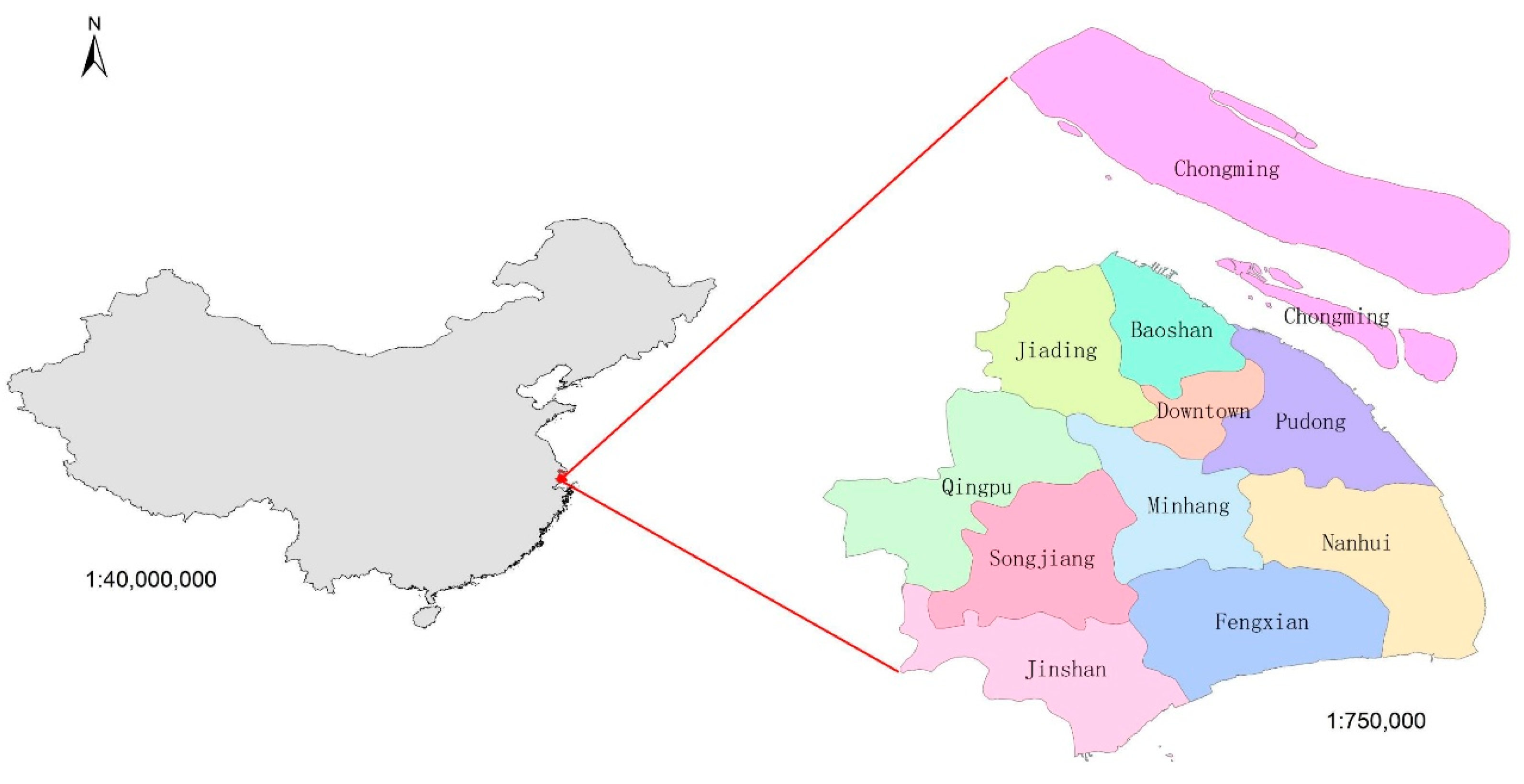
Shanghai is a municipality and one of the first open coastal cities in China. It is located at the confluence of the Yangtze River and Huangpu River and in the center of China’s north and south coast. Shanghai is a part of the alluvial plain of the Yangtze River Delta. The Yangtze River Delta city group, comprising Shanghai, Jiangsu, Zhejiang and Anhui provinces, has become one of the six major world-class city groups.
Shanghai administers 16 municipal districts covering a total area of 6340 square kilometers. Shanghai, which has a subtropical humid monsoon climate, exhibits the characteristics of four distinct seasons, full sunshine and abundant rainfall. Table 1 gives detailed climate information for Shanghai which is presented on the website of EnergyPlus [36]. All the climate data for Shanghai were obtained based on the decades of statistical climate data (1983 to 2010).
Shanghai is China’s economic, transportation, technological, industrial, finance, trade, exhibition and shipping center. The throughput of cargo and containers in Shanghai ranks first in the world. As the world’s leading financial center, Shanghai’s GDP ranked first among China’s cities and second among Asian cities in 2015, second only to that of Tokyo, Japan. Shanghai is an immigrant city. Its unique conditions have attracted a large number of people over the long history of its development process as this sea town has become a world metropolis. By the end of 2016, the population of Shanghai was 24.197 million. Figure 2 shows the location of Shanghai in China.
2.2. Image Data
In this study, all raw image data of Shanghai were downloaded from the United States Geological Survey (USGS) website. Three phases of image data in 2002, 2007 and 2013 all have good quality with no cloud cover found in the selected area.
Table 2 shows the raw data for Shanghai. The images are named after their imaging time by year and day of the year. Every image includes the information of its imaging sensor, date, resolution and wave bands. The OLI image consists of visible bands, the near infrared (NIR) band, thermal infrared (TIR) band and short wave infrared (SWIR) band, which are present in TM images, and also the coastal band, panchromatic (Pan) band and cirrus band. TIRS bands are also thermal infrared bands with a higher resolution compared with TIR bands.
In addition, LST retrieval requires radiometric calibration for thermal band. For TM images, thermal band is band 6. For OLI images, thermal band is band 10 and 11. The specific implementation can be seen in Section 4.4.
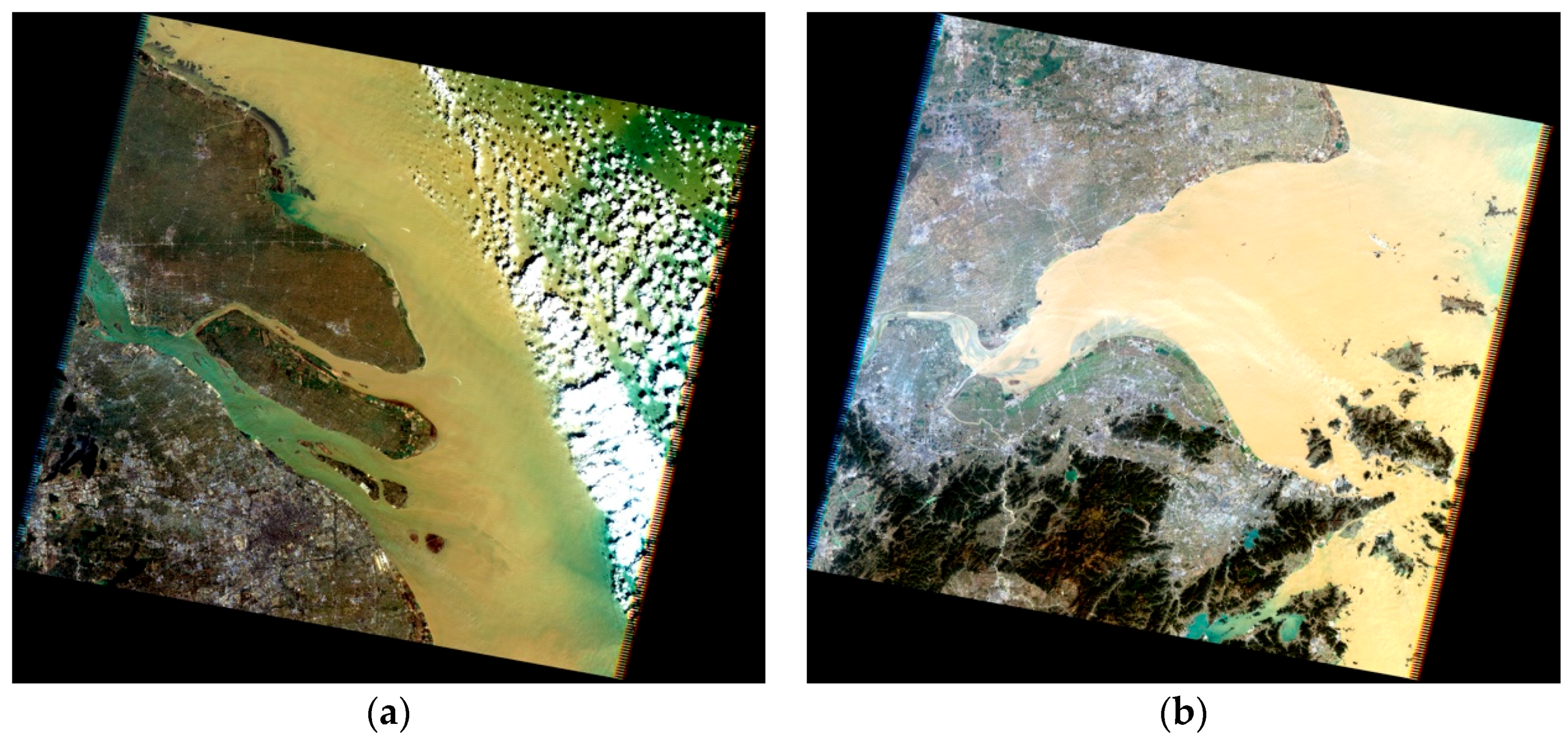
Since the administrative area of Shanghai straddles two Landsat images, a phase of an image for Shanghai has to be mosaicked by two unprocessed images. Figure 3a,b are what they looks like when downloaded who are named after the numbers of air strips and their imaging year and day of the year, demonstrating two examples of unprocessed images for one phase and are displayed in true color.
3. Methodology
3.1. Pre-processing
3.1.1. Radiometric Calibration
Radiometric calibration is used to determine the exact radiation brightness value at the sensor entrance and to further convert the radiance value to the outer surface reflectivity [38]. The formula is presented as follows.
is the radiation value at the sensor entrance for band i. is the brightness value of band i output by the sensor. is the absolute calibration gain coefficient. is the absolute calibration bias value. The values of gain and bias are available in the header file of the remote sensing image.
3.1.2. Atmospheric correction
Atmospheric correction is used to convert the radiation brightness value or the outer surface reflectivity to the actual reflectivity of land surface, and the purpose is to eliminate the error caused by the atmospheric scattering, absorption and reflection. The method used in this project is based on the radiative transfer models.
is the reflectivity formed by the path of molecular scattering and aerosol scattering. is the reflectivity formed by atmospheric absorption. S is the atmospheric spherical albedo. is the reflectivity of the land target object. is the scattering transmittance from the sun to the ground. and are solar altitude and sensor altitude, respectively.
3.2. Impervious Surface
The impervious surface is extracted from the vegetation coverage based on the normalized difference vegetation index (NDVI), combined with the application of the water mask extracted by the modified normalized difference water index (MNDWI).
3.2.1. NDVI
NDVI is an approach to assess whether the target on the ground surface has live green vegetation. The calculation of NDVI is relevant to the red band and near-infrared band because of spectral signatures of vegetation, which can be written as:
The value of NDVI ranges from −1 to +1. The higher the result, the higher the density of green leaves.
3.2.2. MNDWI
In this study, the ratio method is applied to extract water information. The ratio method can make use of the difference of the object in different bands, and then highlight the information by the ratio calculation. The most common water index is the modified difference water index (NDWI) [39]. NDWI is calculated using the difference of the green band and near-infrared band, which effectively eliminates the vegetation information to highlight the water information. However, NDWI neglects the influence caused by construction areas like commercial buildings and housing estates. Considering that urban area covers a lot of the study area, the modified normalized difference water index is applied in this study [40], whose calculation is represented as follows:
The calculation of MNDWI helps to obviously display water regions. The pixel values of water tend to be higher than those of other ground objects.
3.2.3. Extraction of Impervious Surface
The dimidiate pixel model is a commonly used remote sensing estimation model to classify the spectral range of the sample as the dividing line to determine whether the terminal pixel falls into the spectral range of the classification sample [41]. In the estimation of the vegetation coverage ratio, assuming that the pixels completely covered by the vegetation and soil as the dividing line, the vegetation coverage () expression can be obtained according to the NDVI, which reflects the information of vegetation growth status on the ground surface.
can be approximately equal to the maximum value of NDVI, and can be approximately equal to the minimum value of NDVI. Therefore, Equation (5) can be expressed as:
3.3. Land Use Classification
A decision tree based on the CRUISE algorithm is used to classify land use types. The full name of CURISE is classification rule with unbiased interaction selection estimation [42]. It is a statistical decision tree algorithm used for data classification and data mining, in which there are four main features. Each node is divided into multiple child nodes, and the number of child nodes is the total number of response variable classes. The bias when the variable is selected is negligible. The algorithm has a variety of ways to handle missing values. The algorithm can detect the local interaction between the predicted variables.
3.4. Land Surface Temperature
The theoretical method of land surface temperature retrieval is to solve radiative transfer equations, eliminate atmospheric impact, and then obtain the land surface temperature. There are three kinds of commonly used methods: single band algorithms [43,44,45], split window algorithms [43,46,47] and multi-angle algorithms [48,49]. Single band algorithms are effective and need fewer parameters and are thus are used in this study.
Additionally, taking into account the limited scope of the study area and considering that the remote sensing images were taken under clear and cloudless weather conditions, the degree of atmospheric impact in space that is consistent and the relative temperature of the ground temperature distribution would not be affected. Therefore, an image-based inversion algorithm using thermal infrared band is chosen in the study [50]. Specific steps are as follows; the first is to convert the DN value to the radiance value.
is the radiation value at the sensor entrance of the thermal band. is the data value of image pixels. and are the gain coefficient and bias value of thermal band, respectively, which are available from the header file of the remote sensing image.
Second is to convert the radiance value to brightness temperature.
is the brightness temperature, are preset constants before launch.
Third is to calculate the land surface temperature.
is the wavelength of emission radiation and is emissivity.
Due to the complexity of the underlying surface type, for the thermal infrared band with resolution of 60 meters, a pixel corresponding to the underlying surface often contains a variety of materials. Various materials have different emissivity values. Correspondingly, the calculation of emissivity is quite complicated. The following method is used to calculate the emissivity. Firstly, the remote sensing image is divided into three types: the construction land, the water body and the natural ground surface. The emissivity of water pixels is assigned to 0.995. The emissivity of construction land and ground surface is calculated according to formulas (11), (12) and (13) [50]. For a simple calculation, is defined as 0, and is defined as 0.7.
4. Experiment
In the study, the ENVI 5.1 software helps to process and analyze the geospatial remote sensing images and includes both a new interface and classic tools.
4.1. Preprocessing
Due to the limited geographical coverage of a remote sensing image, the Shanghai area should be made up of two remote sensing images. To ensure the comparability of images from different sensors or from the same sensor on different dates, and to eliminate the radiation error caused by atmospheric scattering, the images required radiometric calibration and atmospheric correction. In ENVI, both of these procedures have corresponding operation modules in the toolbox. Then, the projected boundary of Shanghai was imported for the selected regions of interests. Figure 4 shows the result of image preprocessing and is displayed in true color.
4.2. Impervious Surface Extraction
4.2.1. Impervious Surface Calculation
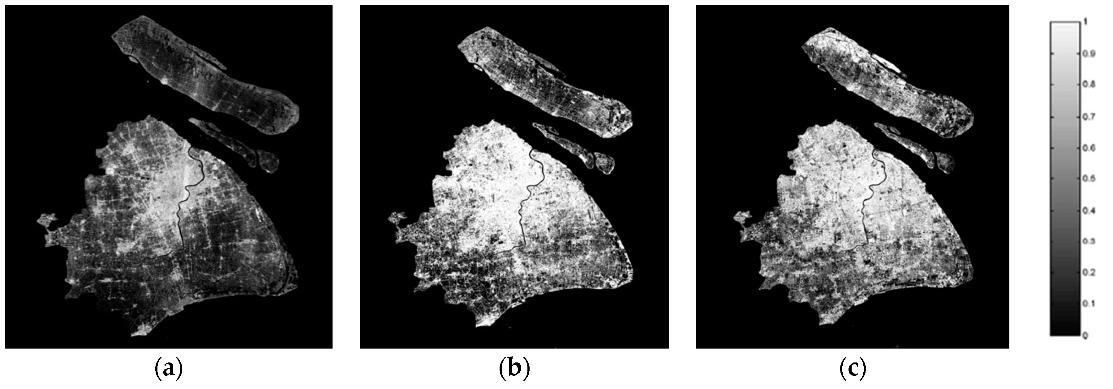
The calculation of NDVI is a ratio operation between the red band and near infrared band. There is no need to input the computational formula in ENVI due to the available tool in the toolbox. For TM images, band 3 is the red band and band 4 is the NIR band, and for OLI images, band 4 is the red band and band 5 is the NIR band. Figure 5 shows the result of NDVI. The lighter or white pixels have a higher probability of live green leaves.
Different from NDVI, there is no ready function for MNDWI. Therefore, it has to be done in band math. The input formula is (b1 − b2)/(b1 + b2). Both for TM and OLI images, b1 is assigned as the green band and b2 is assigned as the middle infrared band. Figure 6 shows the result of MNDVI. The darker or black pixels are regions of water.
According to Section 3.2.3, the formula of impervious surface calculation in band math is 1 − (b1 − NDVImin)/(NDVImax + NDVImin), where b1 is the NDVI result in Section 4.2.1. Because this result has not eliminated the influence of water, masking of water should be applied. The binariation formula is (b1 ge threshold) × 0 + (b1 lt threshold) × 1. Here, b1 is the result of MNDWI calculation. The threshold is 0.92, 0.91 and 0.93 for 2002, 2007 and 2013, respectively. After selection of water, the water mask can be applied on the calculation result of reversed vegetation coverage. Figure 7 shows the result of IS extraction, which demonstrates the expansion of urban impervious surface in Shanghai. The percentages of imperious surface are 19.47%, 36.23% and 37.09% in 2002, 2007 and 2013, respectively as Table 3 displays.
4.2.2. Accuracy Assessment
Based on the ground features of the study area and combining visual interpretation with high resolution of QuickBird images in Shanghai, the ground objects are divided into three categories: impervious surface, water area and vegetation cover area; then, the training samples are determined. Using QuickBird images as reference data, randomly generate 200 sampling points in the three phases of images and check their categories. The random sampling points are compared with the corresponding points in the QuickBird images at the same latitude and longitude to figure out the similarities and differences. Table 4 shows the accuracy.
4.3. Land Use Detection
4.3.1. Classification
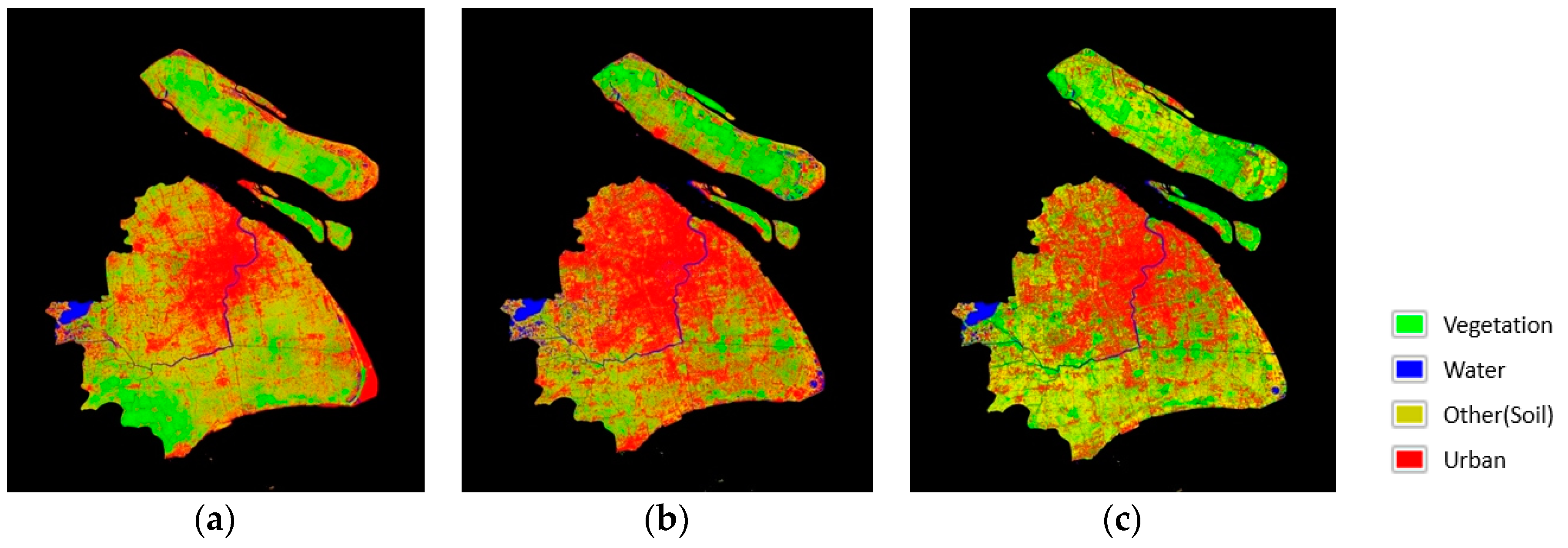
In this experiment, a decision tree classification based on the CRUISE algorithm is used. Before building a new decision tree, classification training samples should be specified. There are four classes, which are vegetation, water, urban and others. In these four classes, urban is defined as an impervious surface while other three classes are pervious land.
Then, the decision trees can be created with the application of the plug-in RuleGen. The trees created by RuleGen tend to be too complex and need to be trimmed.
Figure 8 shows the land use classification results of 2002, 2007 and 2013. The red pixels represent urban areas. The green pixels represent vegetation. The blue pixels represent water. The light-yellow pixels represent other types, mainly bare land.
4.3.2. Confusion Matrix
In this study, the high-resolution QuickBird images are also used to examine the land use classification result of 2002, 2007 and 2013. In ENVI5.1, this procedure can be realized by the module of the confusion matrix using ground truth images. Selecting ground truth images and adding the combination with the four classes lead to the results. Table 5 displays the classification accuracy.
4.4. Land Surface Temperature Retrieval
4.4.1. Calculation Process
Figure 9 shows that land surface temperature retrieval is a complicated process.
To calculate vegetation coverage is a little bit different from Section 4.2.1. The formula input in band math is (b1 gt 0.7) × 1 + (b1 lt 0) × 0 + (b1 ge 0 and b1 le 0.7) × ((b1 − 0)/(0.7 − 0)), where b1 is the NDVI. Then, the calculation result of vegetation coverage is obtained.
Emissivity is a piecewise function, which is divided into water, built-up areas and ground surface. With b1 as NDVI and b2 as vegetation coverage, emissivity is computed according to the band math (b1 le 0) × 0.995 + (b1 gt 0 and b1 lt 0.7) × (0.9589 + 0.086 × b2 − 0.0671 × b2^2) + (b1 ge 0.7) × (0.9625 + 0.0614 × b2 − 0.0461 × b2^2). Then, the calculation result of emissivity is obtained.
The radiance value is relevant to emissivity and the radiometric calibration result for the thermal band. The formula is represented as below, (b2 − 0.86 − 0.87 × (1 − b1) × 1.42)/(0.87 × b1), and b1 is emissivity when b2 is radiometric calibration result for thermal band. Then, the calculation result of radiance value is obtained.
The final step is to compute land surface temperature with the radiance value as b1. For TM images, the formula is (1260.56)/alog (607.66/b1 + 1) − 273.15. For OLI band 10, the formula is (1321.80)/alog (774.89/b1 + 1) − 273.15. For OLI band 11, the formula is (1201.14)/alog (480.89/b1 + 1) − 273.15. The first formula is applicative for images of 2002 and 2007. The later ones are used for 2013. Then, the land surface temperature is obtained.
4.4.2. Land Surface Temperature Intervals
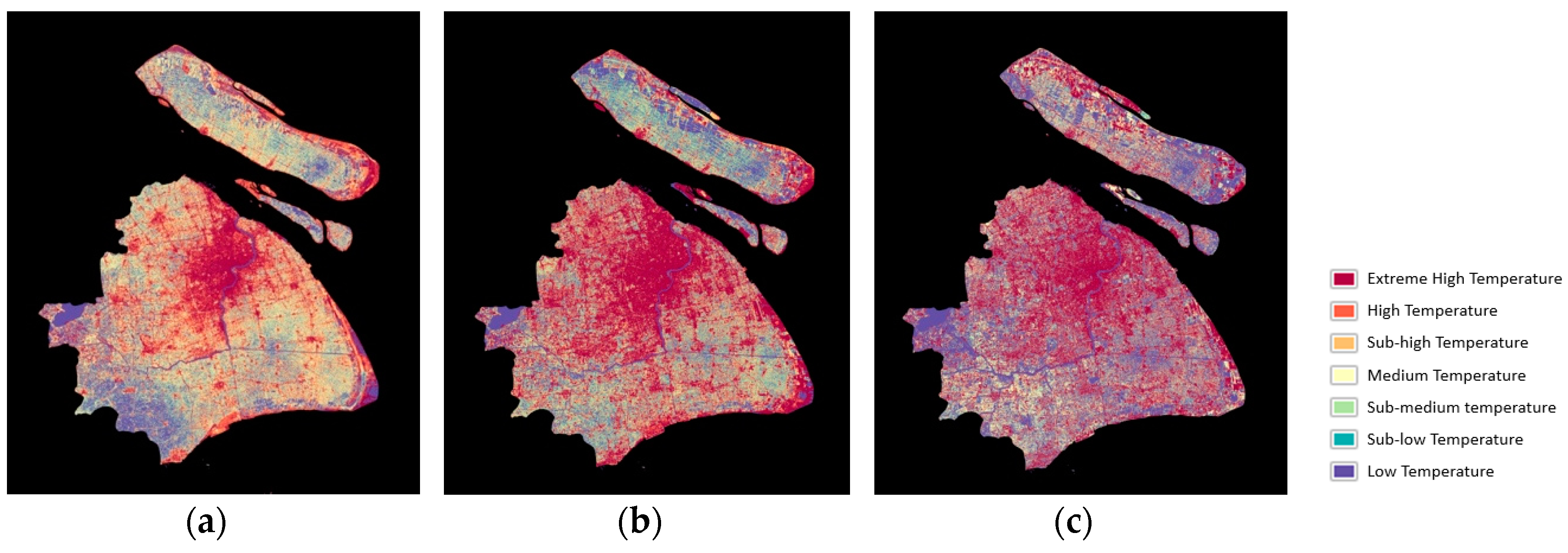
Since the images used in the study are from different years and different months, normalization of land surface temperature is applied for fair comparison. In addition, the temperatures are divided into seven intervals to display the difference of temperature in different regions of Shanghai in 2002, 2007 and 2013. They are low temperature, sub-low temperature, sub-medium temperature, medium temperature, sub-high temperature, high temperature and extreme high temperature. The division rules are shown in Table 6. Figure 10 is the surface urban heat island effect distribution of 2002, 2007 and 2013.
5. Results and Analysis
5.1. Spatial Distribution and Characteristics of Impervious Surface
5.1.1. Impervious Surface Distribution in Shanghai
Impervious surface is one of the main types of land cover in urban areas. It is also an important component of urban ecosystems.
By a series of processes involving the impervious surface, binarization diagrams in different years were obtained (Figure 7). These three pictures vividly revealed that there is a rapid expansion of impervious surface in Shanghai, especially in the city’s center.
In general, the statistical data present an ascending trend from 2002 to 2013. In detail, there is a booming from 2002 to 2007 in terms of proportion, after which the figure for impervious surface remains stable with minute growth from 2007 to 2013, as shown in Table 3.
The expansion of the built-up area depends on the balance between increasing urban construction land scale and the limited environmental capacity of proper conditions, and its developing direction concentrates in a special region. Therefore, the study area is divided into 10 sub-regions according to the administrative division: downtown (including Huangpu, Xuhui, Changning, JingAn, Putuo, Hongkou and Yangpu seven districts), Pudong (include old Pudong and Nanhui), Minhang, Baoshan, Jiading, Jinshan, Songjiang, Qingpu, Fengxian and Chongming districts. The following data analysis will be deeper based on these 10 sub-regions.
After clipping the result for the impervious surface, the entire study area was divided into 10 sub-regions. By binarization processing with the suitable threshold value, the three impervious surface statistics information data were obtained for 2002, 2007 and 2013 in Table 7.
Statistical data of the generated cylindrical statistical diagram can directly reflect the diverse regional impervious surface growth conditions. The development condition of the impervious surface in each period within the study area reflects the significant difference. The transformation of Pudong new district, Jiading, Jinshan, Songjiang, Qingpu and Fengxian districts is most distinct among all sub-regions, which showed an almost twofold increase from 2002 to 2007. Generally, the tendency between 2007 and 2013 is a very small increase in all areas. There is a mild and regular rise in all the non-downtown areas with a great increase in Pudong new district. Specifically, the change in downtown is unusual with a tiny decline partly due to more vegetation covers after the 2010 Expo and its environmental improvement plan.
Table 8 shows the impervious surface proportion table of 10 sub-regions.
In order to proceed with further research of the transformation law based on differences in the regional impervious surface information over time, the three phase of images are divided into two periods (namely 2002–2007, 2007–2013) so we can understand the urban growth over time more specifically. Table 9 lists the impervious surface area growth in two periods. Apparently, there is only a minute decline in downtown areas; conversely, five figures (>100) reflect a dramatic increase in Pudong, Minghang, Jiading, Songjiang and Fengxian districts.
Based on the statistical data above, the growth percentage of the impervious surface in the study area within each period can be calculated, which could represent the overall growth rate of the urban area within two periods. According to Table 10, both downtown and other districts display an obvious increasing rate from 2002 to 2007. In particular, the figures of Pudong new district, Jiading, Jinshan, Songjiang, Qingpu and Fengxian even exceed 100%. From 2007 to 2013, apart from the slight decline for the downtown, the other nine districts all gain slight increase in the coverage of impervious surface.
Generally speaking, with the rapid development of urbanization, the density of buildings in urban built-up areas in Shanghai is quite high, while the greening rate is low. Statistics indicate that the average impervious surface rate in 2013 inside Shanghai’s outer ring road reached 70%, much higher than that of most foreign mega-cities (around 40%).
From the spatial distribution map of impervious surface, it is estimated that the overall impervious surface rate of Shanghai is generally high, especially within the inner ring of the city center, and its impervious surface rate has reached over 90%. In addition, Zhabei and Wusong, industrial zones along Huangpu River, and some of the new industrial areas in Pudong new district have also climbed to more than 85%. There is a significant difference between the urban land outside the inner ring and the downtown area, and its impervious surface rate of ranges from 50% to 85%. Besides, parks and green space in the urban area and the remaining farmland in Pudong new district have an impervious surface rate below 50%.
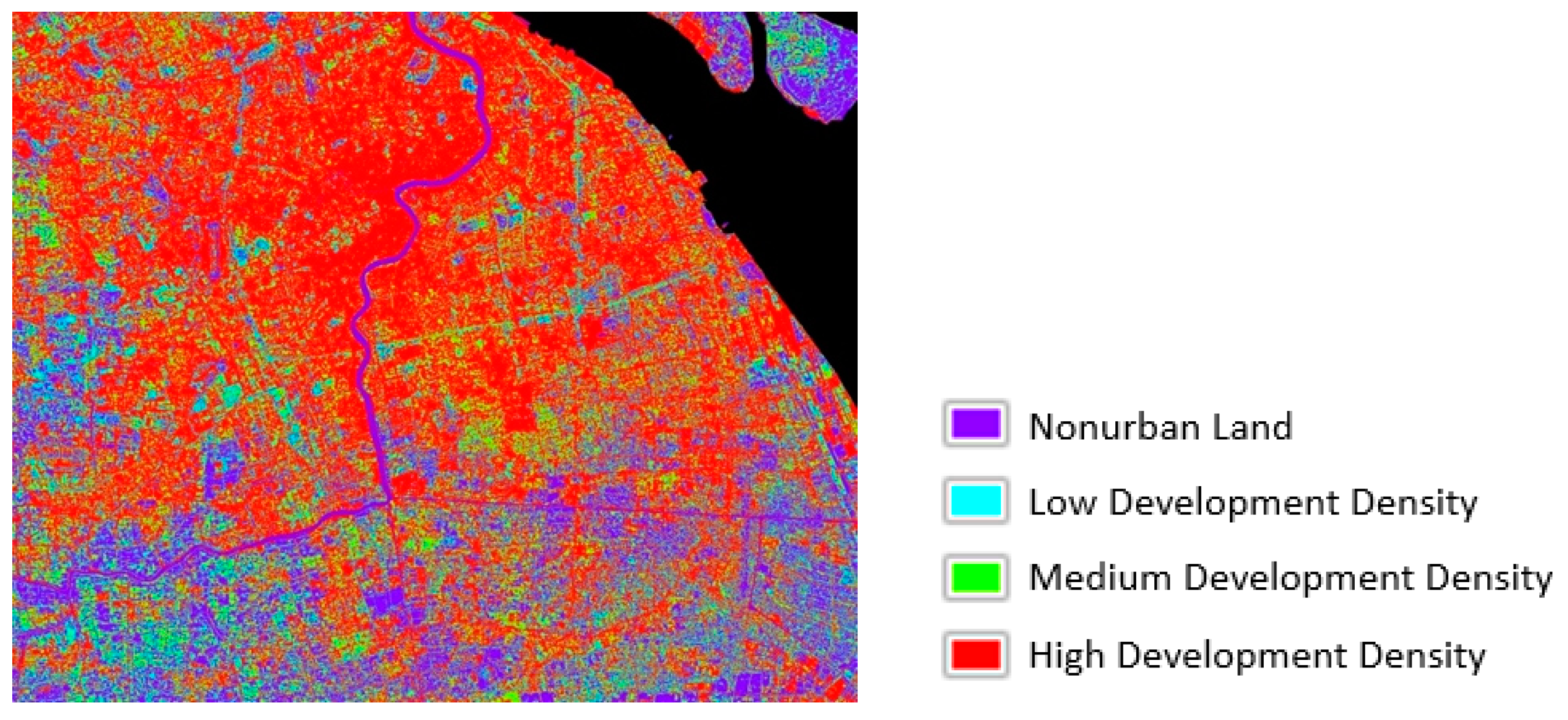
5.1.2. Urban Development Density Analysis
Impervious surface is an important indicator of urban spatial distribution and development density. A previous study reported the characteristics of thermal environment and city development condition in Tampa Bay and Las Vegas, the United States [51], in which the selected regions were the impervious surface rate that included more than 10% as urban land (e.g., 10% to 40% as low, 40% to 60% as medium and 60% to 100% as a high development density area).
Shanghai as one of the largest cities in China has been under high-density development for a long time. Its impervious surface rate is higher than other cities at home and abroad. Therefore, the threshold is different from the above rules. In this study, urban development density is divided into four degrees. Regions whose impervious surface rate is less than 40% are considered as non-urban land, mainly including bare land, farmland and water. Forty to 60% is considered a low development density area. Sixty to 80% is a medium development density area. Eighty to 100% is a high development density area. Selecting the downtown area as regions of interests, Figure 11 shows the distribution of urban development density.
From Figure 11, it is obvious that most area within the inner ring belongs to the high development density areas. Tongji University, People Square, Century Park and the old residential area near Xujiahui are formed into some rarely seen medium development density areas and low development density areas within the inner ring. Medium development density areas are mainly located in the new towns outside the inner ring, except for Wusong Industrial Zone and Zhabei Industrial Zone. Low development density areas are mainly located in Pudong new district and Dachang Town in Baoshan district. In general, the density of urban development is significantly different between the inner ring and outer ring.
5.2. Land-Use and Land-Cover Change
As illustrated in Section 2.2, the images ownloaded in this study were all taken in winter, from December, January and February. Therefore, the accuracy of land use classification depends on the actual situation on that day. The result of land classification (Figure 8) is obtained by the means of a decision tree, which vividly showed a change in urban, water, vegetation and other land (mainly soil), especially in the urban area.
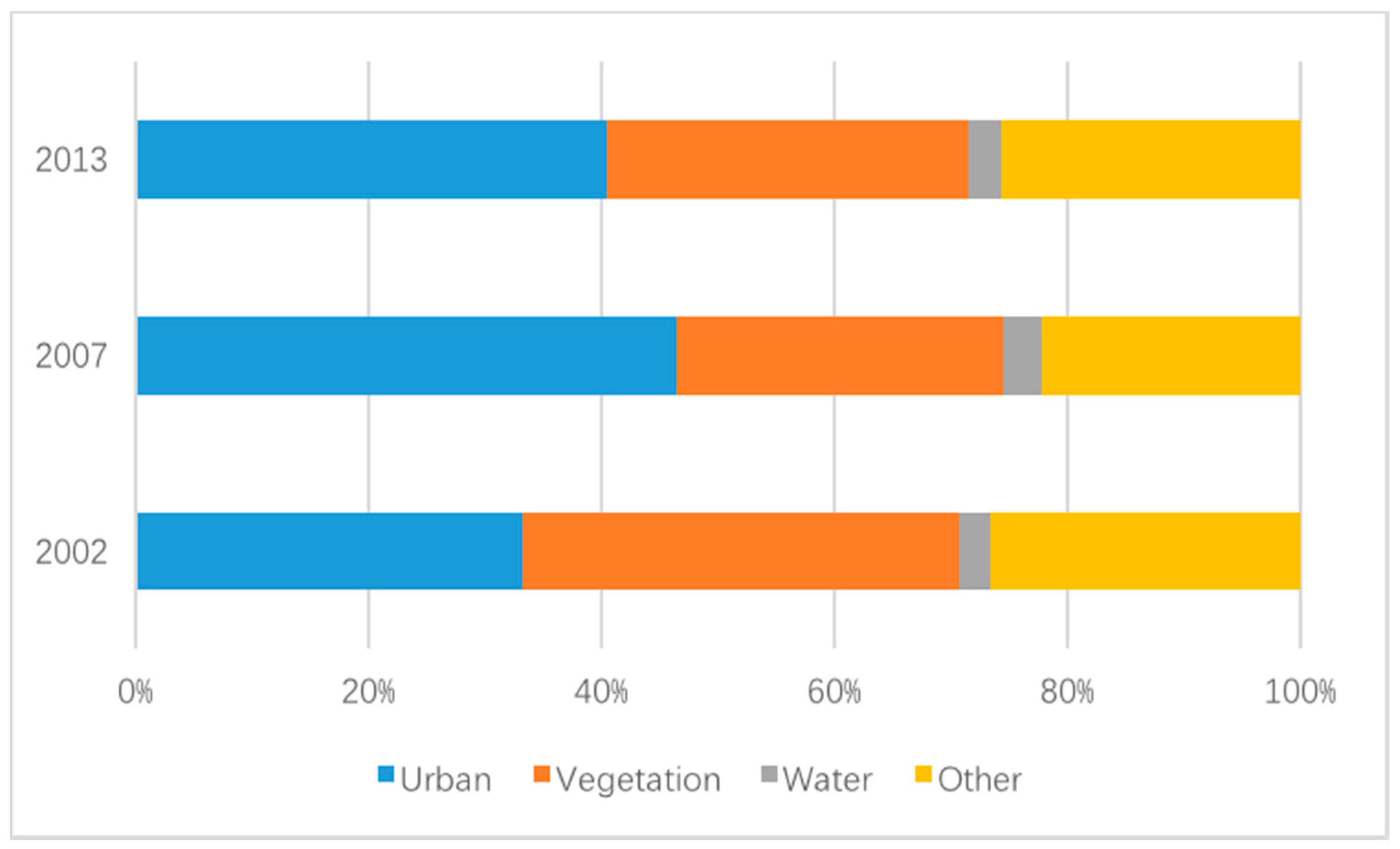
In detail, the data from the Table 11 reflect an increase in terms of urban and water areas from 2002 to 2007, while the figure for urban area declines from 2007 to 2013. The trend also complies with the result of impervious surface extraction. From the proportion diagram (Figure 12), the trend of the greater decrease in vegetation area is quite obvious, as it was from 2002 to 2007. The change in water stays in acceptable ranges.
Through LUCC maps complying with the impervious surface maps in 2002, 2007 and 2013, the regions inside the outer ring were found to be basically urbanized, and only a small amount of farmland existed in Pudong new district. Urban areas gradually replace the original vegetation and soil land. The built-up area of the city center has extremely high coverage and has been under intensive development for a long time.
Furthermore, the average LSTs of four types of land use in 2002, 2007 and 2013 were marked in Figure 12. The difference between the average temperature of urban and vegetation areas in 2007 exhibited a maximum value among the three phases of images, which was exactly in accordance with the differences of their areas. Thus, a general result could be drawn that the missing vegetation coverage that turned into ISA led to the intensifying of SUHI, which also verified the impact of LUCC on LST.
5.3. Surface Urban Heat Island Analysis
5.3.1. Surface Urban Heat Island Intensity Distribution
According to the land surface temperature retrieval result, the temperatures are divided into seven intervals for fair analysis considering that different days in divergent months have different land surface temperatures. The distribution maps are shown in Figure 10. Their main characteristic is that the high temperature zone expands from the central urban area to the outskirts. Through the comparison of SUHI intensity maps, areas of heat islands are shown to increase, mainly in the city’s center and the centers of districts from 2002 to 2007. However, the heat island effect shows signs of abating from 2007 to 2013, and the expansion of the medium temperature zone and sub-high temperature zone generally focuses on Pudong, Nanhui and Fengxian. The area of extreme high temperature zones and high temperature zones is decreasing, and their distribution becomes scattered, not solely focusing on the city’s center and centers of districts. Low temperature zones are located in the outskirts of Shanghai, mainly in Fengxian, Jinshan and parts of Pudong and Nanhui.
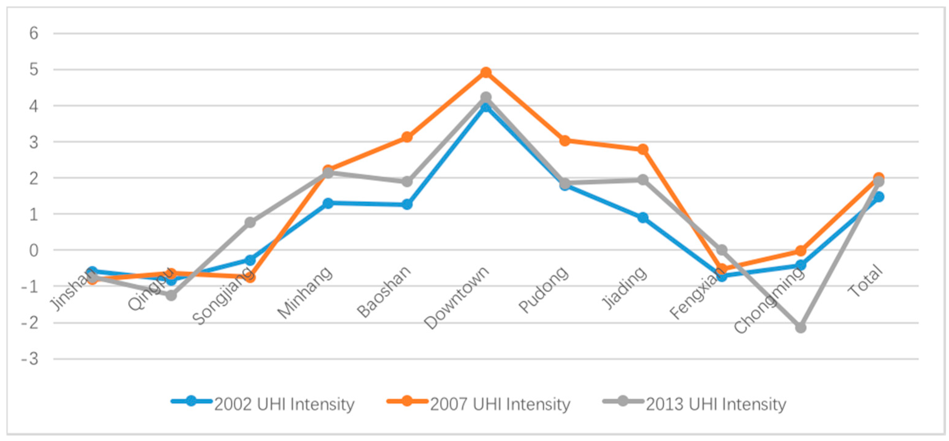
To test the phenomenon that the heat island intensity first increased and then decreased, the heat island intensity of the city center and nine other districts was extracted in this study. Here is the calculation formula of the SUHI intensity:
is the average temperature of the downtown area. is the average temperature of outskirts, and outskirts are defined as regions outside the outer ring. is the standard deviation of temperatures.
Table 12 shows the average LSTs and SUHI intensities of the downtown area and the remaining districts in Shanghai. Obviously, at the imaging time, the average LSTs and SUHI intensities both declined from downtown to outskirts. It is known that LSTs vary in different seasons or even at different times on the same day, and winter nights exhibit the most intensive SUHI in Shanghai due to the specific location and structure [52]. Therefore, the result of winter is chosen to distinctly analyze the relationship of LST and LUCC.
Figure 13 demonstrates that the heat island intensity gradually decreases from the city center to the suburbs, and reaches the maximum positive value in the city center, while the heat island intensity in the outer suburbs is negative. From the trend of the entire curve, it is easy to see that the heat island effect is the strongest in 2007, while in 2013, it dropped slightly.
Statistics from Shanghai Municipal Statistics Bureau show that the completed construction area in 2002 was 18.8 million square meters, and the figure reached 28.43 million square meters in 2007 while it declined into 14.39 million square meters in 2013 [53]. On the other hand, the resident population of Shanghai was 17.13, 20.64 and 24.15 million in 2002, 2007 and 2013, respectively [52]. Both the urban construction and increasing population and human activities contribute to the intensity of the heat island effect. Therefore, the SUHI effect was particularly evident in 2009. Nevertheless, with the coming Expo in 2010, Shanghai not only carried out more rational planning for urban construction but also made a breakthrough in the ecological environmental construction. This progress was maintained after the Expo in 2010. Therefore, the SUHI effect was not that intensive in 2013.
5.3.2. Correlation Analysis of SUHI and IS, LUCC
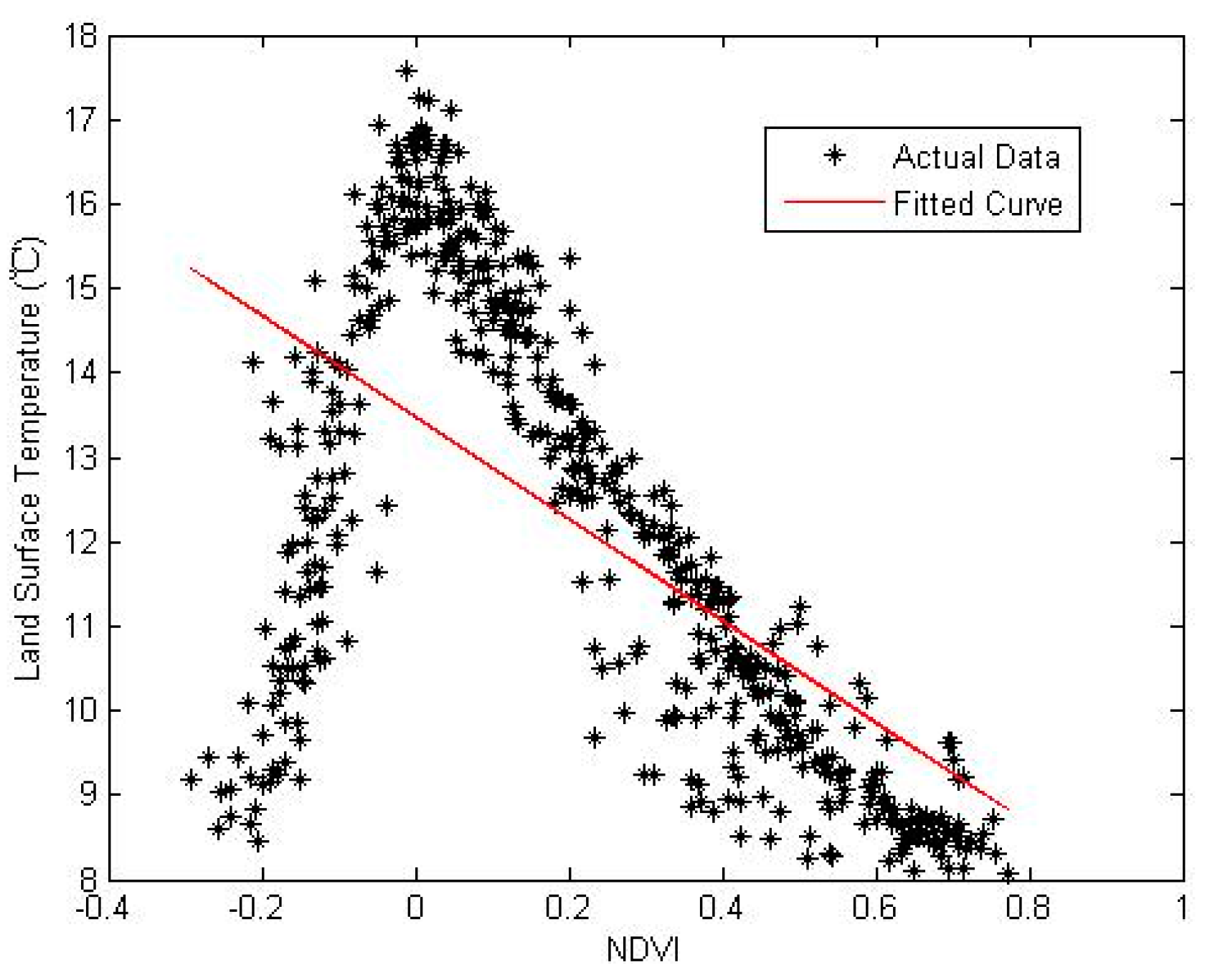
SUHI is a local climate characteristic affected by global climate change and is determined by human factors and local geographical conditions. The land surface temperature is closely related to the land cover which is an important factor leading to the SUHI. In urban built-up areas, land cover types are mainly impervious surface, vegetation and water. These three ecological factors, meteorological factors, artificial heat have a comprehensive impact on the SUHI effect. Therefore, this section will demonstrate the correlation between LST and IS, NDVI, MNDWI in 2013 with the help of MATLAB software.
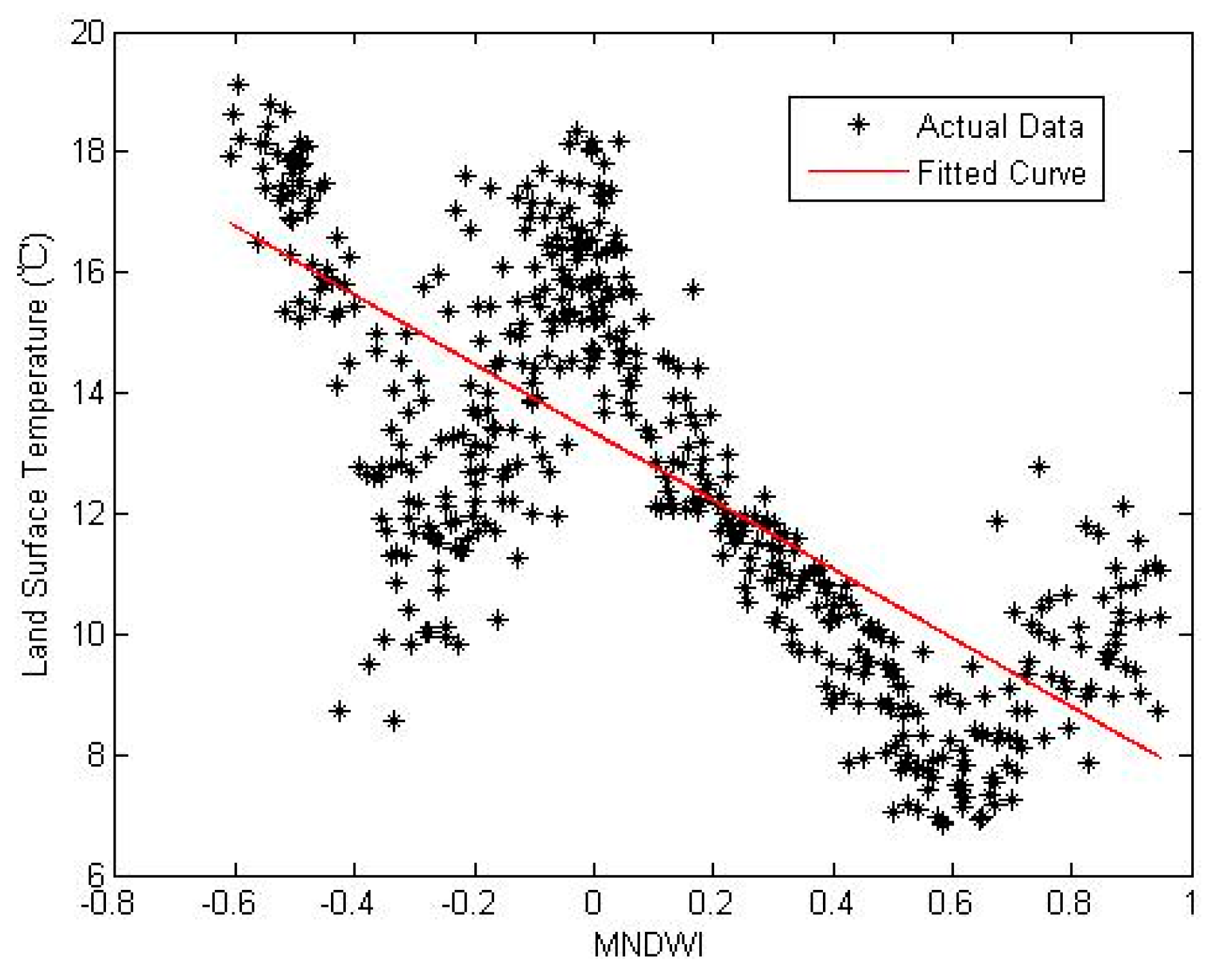
A total of 500 sample points were randomly generated by means of MATLAB. The impervious surface rates, NDVI values, MNDWI values and corresponding land surface temperature were used to show the relationships (Figure 14, Figure 15 and Figure 16).
In the correlation analysis of IS and LST, both linear fitting and quadratic fitting gave a high goodness of fit.
,
,
The linear fitting model passed the F test and the t test under the 95% confidence interval. The regression coefficient is positive, which means that the impervious rate has a linear positive correlation with land surface temperature. That is, land surface temperature increases with the addition of the impervious surface rate.
As for the correlation analysis of NDVI and LST, an apparent linear or exponential correlation does not exist, while a negative trend does. In addition, where rocks and brick exist (NDVI = 0) has higher land surface temperature, while vegetation-covered land (NDVI > 0.7) and water (NDVI around 0.2) have lower land surface temperatures, which become the cold island in Shanghai.
As for the correlation analysis of MNDWI and LST, the value of LST generally drops in accordance with the increasing value of MNDWI. When the MNDWI value is greater than 0.6, it has lower land surface temperature. Therefore, MNDWI and LST also have a negative correlation, which is not that obvious. The temperatures are distinct depending on regional conditions.
Generally speaking, impervious surface has a positive correlation with land surface temperature and is the strongest between the three factors. Vegetation and water have negative correlations with land surface temperature, and vegetation is more relevant than water.
6. Discussion
With the development of urbanization especially in developing countries, buildings and structures have been continuously built over decades. The resulting increase of impervious surface area and decline of water and vegetation have gradually affected land surface temperature and contributed to the SUHI effect.
Studies demonstrate that IS has a warming effect which is a key indicator in urban planning [28,29,30], consistent with the conclusion of this study. Xu stated that LST and IS have exponential relationships [28], while Cao illustrated their linear positive correlation [30]. Based on the conclusion drawn from Figure 14, both linear fitting and quadratic fitting methods showed a high goodness of fit. This means that an exponential correlation exists due to variations of imaging time and actual on-site conditions.
In comparison, vegetation and water are able to cool the built-up area. Yuan and Zhou both reported that NDVI has a negative linear correlation with LST [26,27], while Yuan argued that it was a weak correlation, similar to our result in this study. Cao also demonstrated that MNDWI has a strong negative linear correlation with LST [30], but our study shows a weaker dependency than IS.
Nonetheless, slight differences among similar studies are possible. As mentioned above, the images used in this paper were from winter nights. Since the underlying surface of Shanghai transforms from season to season, the change of surface structure led to the variation of LSTs. Thus, the specific exponential relationships or their power might be a little different although they share the same trends between LUCC and LST.
7. Conclusions
In this study, we analyzed the general trend of impervious surface growth from 2002 to 2007 and its minor increase from 2007 to 2013. The greatest increase in the impervious surface was from farmland, causing a loss of vegetation coverage and leading, to a certain degree, to local SUHI effects. Simulations also demonstrate that the relationship between LST and IS is a positive correlation, while the relationships with NDVI and MNDVI are negative. This result means that the construction of impervious surface strengthens the SUHI effect, while vegetation and water bring about some degree of relief.
Conversely, the driving force of land-use change varies, including the influence of policy, economy, population distribution, and the effect of climate or topography. In short, with the rapid development of urbanization, the policy implications for land use and the control of impervious surface should receive more attention from the urban planning and design used in Shanghai in the future.
The remote sensing data used in this study are images from winter for determining the influence of vegetation shades, which leads to the seasonal influence on the SUHI effect being ignored. Therefore, analysis of different seasons is taken into consideration in the future study. This study focuses on the macroscale problem, which is the speculated relationship between SUHI and IS, water and vegetation. In the near future, it is still necessary to include multiple factors such as ventilation and microclimate for further study in local areas of Shanghai. Moreover, multi-date meteorological data should be introduced to determine how synoptic conditions synergistically affect SUHI.
Acknowledgments
The data from the USGS website and from the local government of Shanghai are highly appreciated. This research is jointly supported by the National Key Research and Development Program of China (Project Ref. No. 2016YFB0501501) and the Natural Scientific Foundation of China (41471353).
Author Contributions
Haiting Wang and Yuanzhi Zhang conceived, designed and performed the experiments, analyzed the data, and wrote the paper; Yu Li improved the data analysis; Jin Yeu Tsou contributed reagents/materials/analysis tools.
Conflicts of Interest
The authors declare no conflict of interest.
References
- Heilig, G.K. World Urbanization Prospects: The 2011 Revision; United Nations, Department of Economic and Social Affairs (DESA), Population Division, Population Estimates and Projections Section: New York, NY, USA, 2012. [Google Scholar]
- Reid, R.S.; Kruska, R.L.; Muthui, N.; Taye, A.; Wotton, S.; Wilson, C.J.; Mulatu, W. Land-use and land-cover dynamics in response to changes in climatic, biological and socio-political forces: The case of southwestern Ethiopia. Landsc. Ecol. 2000, 15, 339–355. [Google Scholar] [CrossRef]
- Huang, J.; Zhao, X.; Tang, L.; Qiu, Q. Analysis on spatiotemporal changes of urban thermal landscape pattern in the context of urbanisation: A case study of Xiamen City. Shengtai Xuebao/Acta Ecol. Sin. 2012, 32, 622–631. [Google Scholar] [CrossRef]
- Alavipanah, S.; Wegmann, M.; Qureshi, S.; Weng, Q.; Koellner, T. The role of vegetation in mitigating urban land surface temperatures: A case study of Munich, Germany during the warm season. Sustainability 2015, 7, 4689–4706. [Google Scholar] [CrossRef]
- Giorgio, G.A.; Ragosta, M.; Telesca, V. Climate variability and industrial-suburban heat environment in a Mediterranean area. Sustainability 2017, 9, 775. [Google Scholar] [CrossRef]
- Wang, J.; Da, L.; Song, K.; Li, B.L. Temporal variations of surface water quality in urban, suburban and rural areas during rapid urbanization in Shanghai, China. Environ. Pollut. 2008, 152, 387–393. [Google Scholar] [CrossRef] [PubMed]
- Cao, K. Analysis of urban rain island effect in shanghai and its changing trend. Water Resour. Power 2009, 5, 31–33. [Google Scholar]
- Kim, H.H. Urban heat island. Int. J. Remote Sens. 1992, 13, 2319–2336. [Google Scholar] [CrossRef]
- Bornstein, R.D. Observations of the urban heat island effect in New York City. J. Appl. Meteorol. 1968, 7, 575–582. [Google Scholar] [CrossRef]
- Magee, N.; Curtis, J.; Wendler, G. The urban heat island effect at Fairbanks, Alaska. Theor. Appl. Climatol. 1999, 64, 39–47. [Google Scholar] [CrossRef]
- Morris, C.J.G.; Simmonds, I.; Plummer, N. Quantification of the influences of wind and cloud on the nocturnal urban heat island of a large city. J. Appl. Meteorol. 2001, 40, 169–182. [Google Scholar] [CrossRef]
- Ackerman, B. Temporal march of the Chicago heat island. J. Clim. Appl. Meteorol. 1985, 24, 547–554. [Google Scholar] [CrossRef]
- Jusuf, S.K.; Wong, N.H.; Hagen, E.; Anggoro, R.; Hong, Y. The influence of land use on the urban heat island in Singapore. Habitat Int. 2007, 31, 232–242. [Google Scholar] [CrossRef]
- Sarkar, H. Study of land cover and population density influences on urban heat island in tropical cities by using remote sensing and GIS: A methodological consideration. In Proceedings of the 3rd FIG Regional Conference, Jakarta, Indonesia, 3–7 October 2004. [Google Scholar]
- Jincai, D.; Zhikai, Z.; Hong, X.; Hongmei, Z. A study of the high temperature distribution and the heat island effect in the summer of the Shanghai area. Chin. J. Atmos. Sci. Chin. Ed. 2002, 26, 420–431. [Google Scholar]
- Yue, W.; Xu, J.; Xu, L. Impact of human activities on urban thermal environment in Shanghai. Acta Geogr. Sin. 2008, 63, 247–256. [Google Scholar]
- Hao, L.P.; Fang, Z.F.; Li, Z.L.; Liu, Z.Q.; He, J.H. The inter-annual climate change and heat island effect of Chengdu during the recent fifty years. Sci. Meteor. Sin. 2007, 27, 648–654. [Google Scholar]
- Yang, B. Progress of urban heat island effect. J. Meteorol. Environ. 2013, 2, 101–106. [Google Scholar]
- Bai, Z.P.; Qi, T. Monitoring “heat island effect” in urban regions. Cities Disaster Reduct. 2004, 2, 27–28. [Google Scholar]
- Zhao, K.X. Current situation and countermeasures of urban heat island effect. Chin. Landsc. Archit. 1999, 6, 44–45. [Google Scholar]
- Wang, G.X.; Shen, X.L. On the relationship between urbanization and heat island effect in Shanghai. J. Subtrop. Res. Environ. 2010, 5, 1–11. [Google Scholar]
- Chen, X.L.; Zhao, H.M.; Li, P.X.; Yin, Z.Y. Remote sensing image-based analysis of the relationship between urban heat island and land use/cover changes. Remote Sens. Environ. 2006, 104, 133–146. [Google Scholar] [CrossRef]
- Weng, Q.; Lu, D.; Schubring, J. Estimation of land surface temperature–vegetation abundance relationship for urban heat island studies. Remote Sens. Environ. 2004, 89, 467–483. [Google Scholar] [CrossRef]
- Sailor, D.J. Simulated urban climate response to modifications in surface albedo and vegetative cover. J. Appl. Meteorol. 1995, 34, 1694–1704. [Google Scholar] [CrossRef]
- Arnfield, A.J. Two decades of urban climate research: A review of turbulence, exchanges of energy and water, and the urban heat island. Int. J. Climatol. 2003, 23, 1–26. [Google Scholar] [CrossRef]
- Yuan, F.; Bauer, M.E. Comparison of impervious surface area and normalized difference vegetation index as indicators of surface urban heat island effects in Landsat imagery. Remote Sens. Environ. 2007, 106, 375–386. [Google Scholar] [CrossRef]
- Zhou, Y.; Shi, T.M.; Yuan-Man, H.U.; Gao, C.; Liu, M. Relationships between land surface temperature and normalized difference vegetation index based on urban land use type. Chin. J. Ecol. 2011, 30, 1504–1512. [Google Scholar]
- Xu, H.Q. Quantitative analysis on the relationship of urban impervious surface with other components of the urban ecosystem. Acta Ecol. Sin. 2009, 29, 2456–2462. [Google Scholar]
- Lin, Y.S.; Xu, H.Q.; Zhou, R. A study on urban impervious surface area and its relation with urban heat island: Quanzhou city, China. Remote Sens. Technol. Appl. 2007, 22, 14–19. [Google Scholar]
- Cao, L.; Hu, W.H.; Meng, X.L.; Li, J.X. Relationships between land surface temperature and key landscape elements in urban area. Chin. J. Ecol. 2011, 30, 2329–2334. [Google Scholar]
- Mu, H.Z.; Kong, C.Y.; Tang, X.; Ke, X.X. Preliminary analysis of temperature change in Shanghai and urbanization impacts. J. Trop. Meteorol. 2008, 24, 673–674. [Google Scholar]
- Li, D.; Bou-Zeid, E. Quality and sensitivity of high-resolution numerical simulation of urban heat islands. Environ. Res. Lett. 2014, 9, 055001. [Google Scholar] [CrossRef]
- Voogt, J.A.; Oke, T.R. Thermal remote sensing of urban climates. Remote Sens. Environ. 2003, 86, 370–384. [Google Scholar] [CrossRef]
- Quattrochi, D.A.; Luvall, J.C.; Rickman, D.L.; Estes, M.G.; Laymon, C.A.; Howell, B.F. A decision support information system for urban landscape management using thermal infrared data: Decision support systems. Photogramm. Eng. Remote Sens. 2000, 66, 1195–1207. [Google Scholar]
- Picón, A.J.; Vásquez, R.; González, J.; Luvall, J.; Rickman, D. Use of remote sensing observations to study the urban climate on tropical coastal cities. Rev. Umbral (Etapa IV Colecc. Complet.) 2017, 1, 218–232. [Google Scholar]
- EnergyPlus. Available online: https://energyplus.net/weather-location/asia_wmo_region_2/CHN/ (accessed on 25 May 2017).
- United States Geological Survey. Available online: https://www.usgs.gov (accessed on 3 April 2017).
- Zhou, J.Q.; Ye, Q.; Shao, Y.S.; Zhu, S.L.; Guan, Z.Q. Principles and Application of Remote Sensing; Wuhan University Press: Wuhan, China, 2014. [Google Scholar]
- McFeeters, S.K. The use of the Normalized Difference Water Index (NDWI) in the delineation of open water features. Int. J. Remote Sens. 1996, 17, 1425–1432. [Google Scholar] [CrossRef]
- Xu, H. A study on information extraction of water body with the modified normalized difference water index (MNDWI). J. Remote Sens. 2005, 9, 589–595. [Google Scholar]
- Leprieur, C.; Verstraete, M.M.; Pinty, B. Evaluation of the performance of various vegetation indices to retrieve vegetation cover from AVHRR data. Remote Sens. Rev. 1994, 10, 265–284. [Google Scholar] [CrossRef]
- Kim, H.; Loh, W.Y. Classification trees with unbiased multiway splits. J. Am. Stat. Assoc. 2001, 96, 589–604. [Google Scholar] [CrossRef]
- Jiménez-Muñoz, J.C.; Sobrino, J.A.; Skoković, D.; Mattar, C.; Cristóbal, J. Land surface temperature retrieval methods from Landsat-8 thermal infrared sensor data. IEEE Geosci. Remote Sens. Lett. 2014, 11, 1840–1843. [Google Scholar] [CrossRef]
- Copertino, V.A.; Pierro, M.D.; Scavone, G.; Telesca, V. Comparison of algorithms to retrieve lst from LANDSAT-7 ETM+ IR data in the Basilicata Ionian band. Tethys J. Weather Clim. West. Mediterr. 2002, 25–34. [Google Scholar]
- Sobrino, J.A.; Jiménez-Muñoz, J.C.; Paolini, L. Land surface temperature retrieval from LANDSAT TM 5. Remote Sens. Environ. 2004, 90, 434–440. [Google Scholar] [CrossRef]
- Jiménez-Muñoz, J.C.; Sobrino, J.A. A generalized single-channel method for retrieving land surface temperature from remote sensing data. J. Geophys. Res. Atmos. 2003, 108, 2015–2023. [Google Scholar] [CrossRef]
- Zhang, X.; Zhu, Q.J.; Min, X.J. Analysis of split window algorithms for estimating land surface temperature from AVHRR data. J. Image Gr. 1999, 4, 595–599. [Google Scholar]
- Prata, A.J. Land surface temperatures derived from the advanced very high resolution radiometer and the along-track scanning radiometer. J. Geophys. Res. Atmos. 1993, 981, 16689–16702. [Google Scholar] [CrossRef]
- Sobrino, J.A.; Li, Z.; Stoll, M.P.; Becker, F. Multi-channel and multi-angle algorithms for estimating sea and land surface temperature with ATSR data. Int. J. Remote Sens. 1996, 17, 2089–2114. [Google Scholar] [CrossRef]
- Ding, F.; Xu, H.Q. Comparison of three algorithms for retrieving land surface temperature from LANDSAT TM thermal infrared band. J. Fujian Normal Univ. (Nat. Sci. Ed.) 2008, 24, 91–96. [Google Scholar]
- Xian, G.; Crane, M. An analysis of urban thermal characteristics and associated land cover in Tampa Bay and Las Vegas using Landsat satellite data. Remote Sens. Environ. 2006, 104, 147–156. [Google Scholar] [CrossRef]
- Zhang, Y.; Bao, W.J.; Qi, Y.U. Study on seasonal variations of the urban heat island and its interannual changes in a typical Chinese megacity. Chin. J. Geophys. 2012, 55, 1121–1128. [Google Scholar]
- Shanghai Municipal Statistics Bureau. 2017. Available online: http://www.stats-sh.gov.cn/frontinfo/staticPageView.xhtml?para=ldcy (accessed on 25 May 2017).
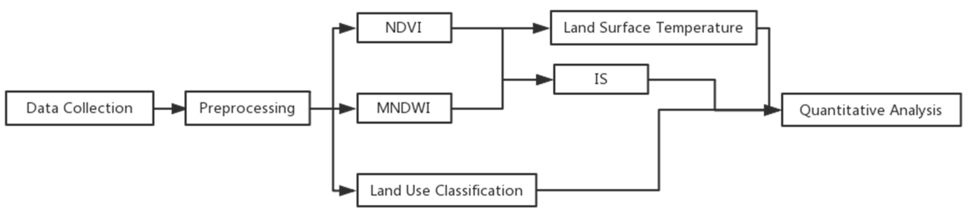
Figure 1.
Flow chart of data processing.

Figure 2.
The location of Shanghai, China.

Figure 3.
Examples of original images with row/column numbers: (a) 1180382007033; (b) 1180392007033.
Figure 3.
Examples of original images with row/column numbers: (a) 1180382007033; (b) 1180392007033.

Figure 4.
(a) Preprocessing result of 2002; (b) Preprocessing result of 2007; (c) Preprocessing result of 2013.
Figure 4.
(a) Preprocessing result of 2002; (b) Preprocessing result of 2007; (c) Preprocessing result of 2013.
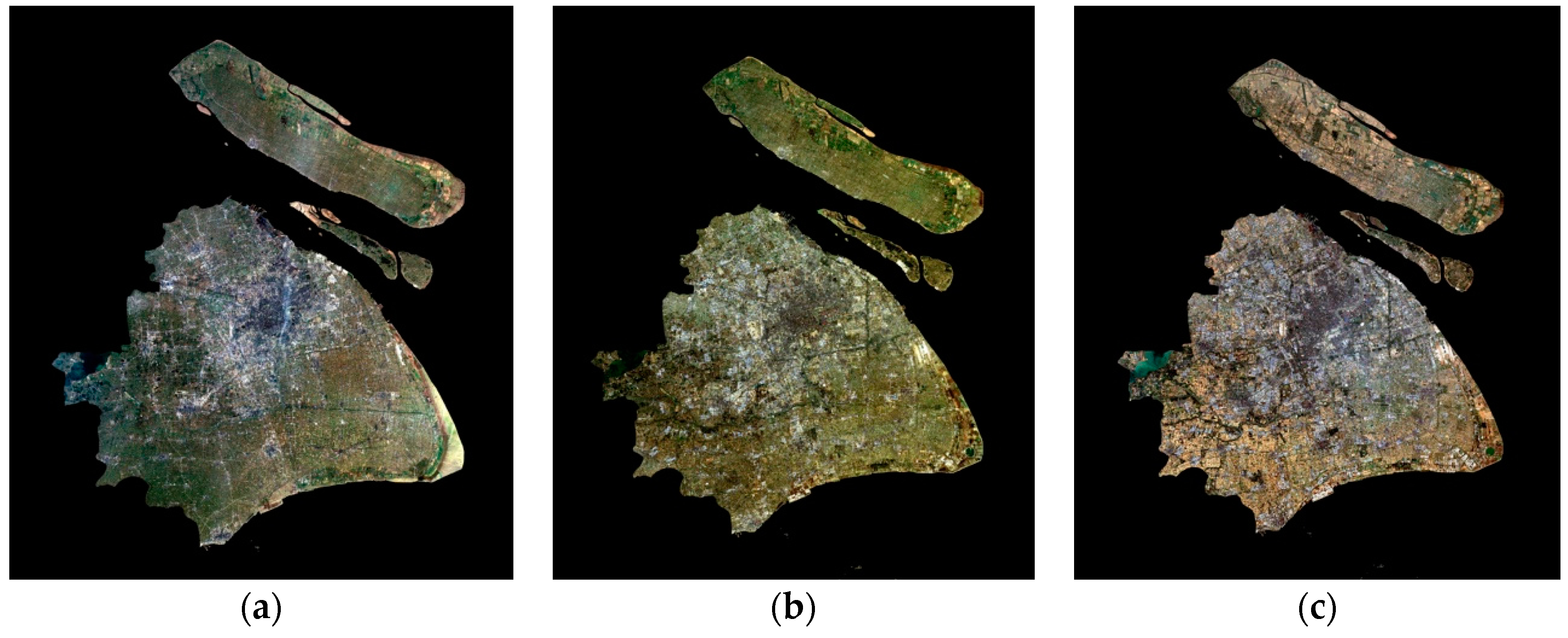
Figure 5.
(a) NDVI calculation of 2002; (b) NDVI calculation of 2007; (c) NDVI calculation of 2013.
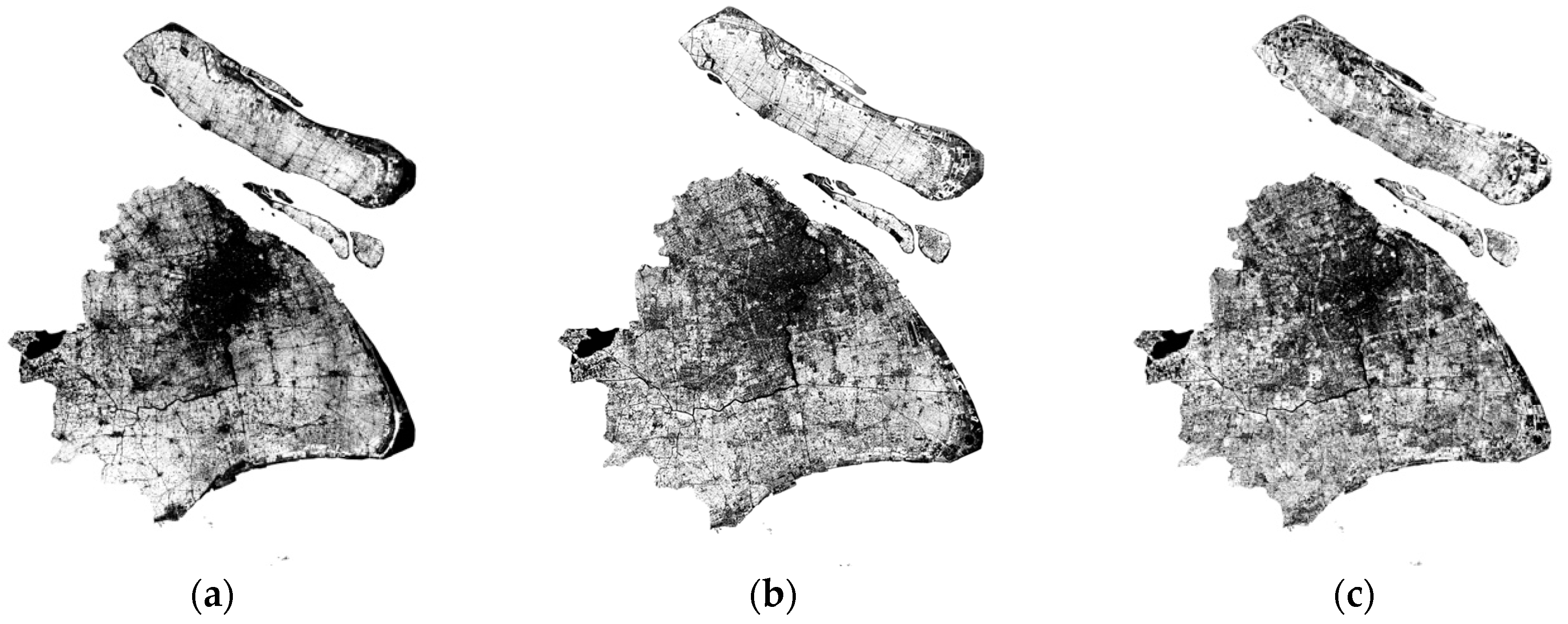
Figure 6.
(a) MNDVI calculation of 2002; (b) MNDVI calculation of 2007; (c) MNDVI calculation of 2013.
Figure 6.
(a) MNDVI calculation of 2002; (b) MNDVI calculation of 2007; (c) MNDVI calculation of 2013.
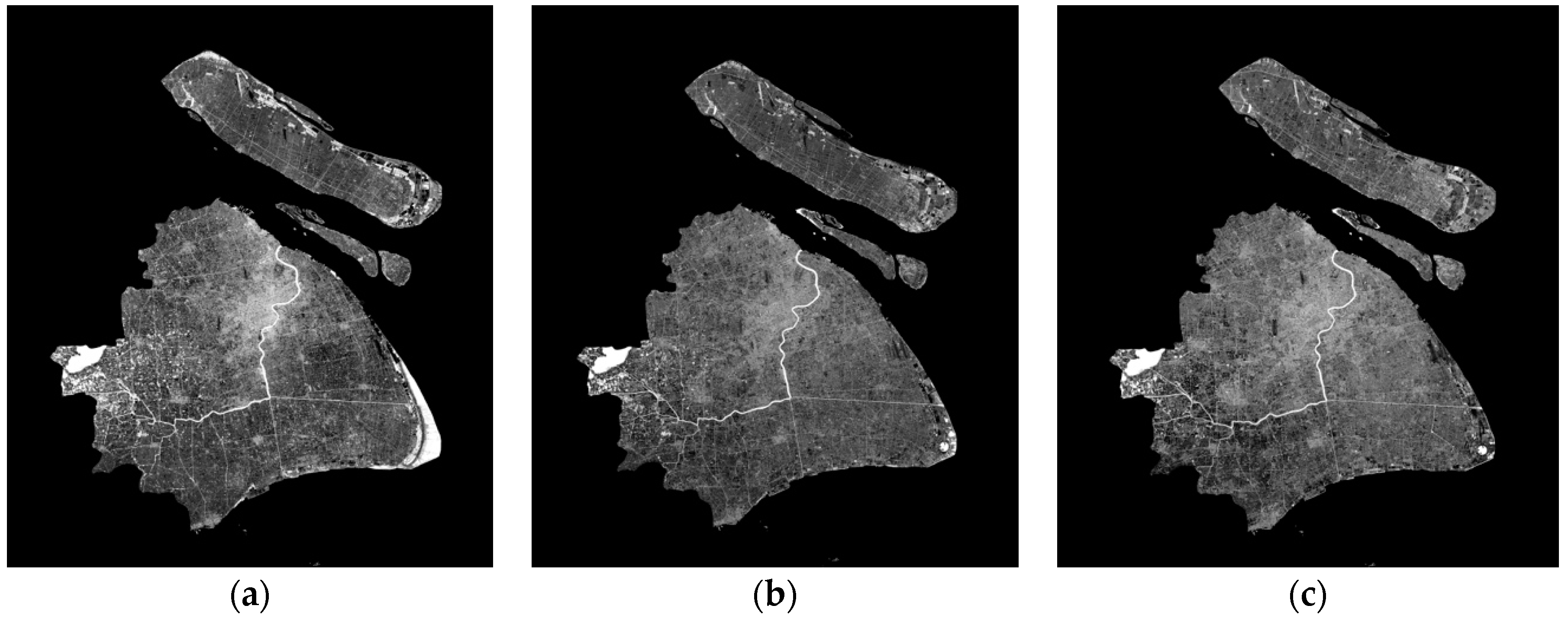
Figure 7.
(a) IS extraction result of Shanghai in 2002; (b) IS extraction result of Shanghai in 2007; (c) IS extraction result of Shanghai in 2013.
Figure 7.
(a) IS extraction result of Shanghai in 2002; (b) IS extraction result of Shanghai in 2007; (c) IS extraction result of Shanghai in 2013.

Figure 8.
Land use of Shanghai in 2002; (b) Land use of Shanghai in 2007; (c) Land use of Shanghai in 2013.
Figure 8.
Land use of Shanghai in 2002; (b) Land use of Shanghai in 2007; (c) Land use of Shanghai in 2013.

Figure 9.
Flow chart of the procedures of land surface temperature retrieval.
Figure 10.
Distribution of urban heat island effect of 2002; (b) Distribution of urban heat island effect of 2007; (c) Distribution of urban heat island effect of 2013.
Figure 10.
Distribution of urban heat island effect of 2002; (b) Distribution of urban heat island effect of 2007; (c) Distribution of urban heat island effect of 2013.

Figure 11.
Distribution of urban development density.

Figure 12.
LUCC proportion diagram.

Figure 13.
Changing of heat island intensity in different districts.

Figure 14.
(a) Relationship between IS and LST; (b) Relationship between IS and LST.
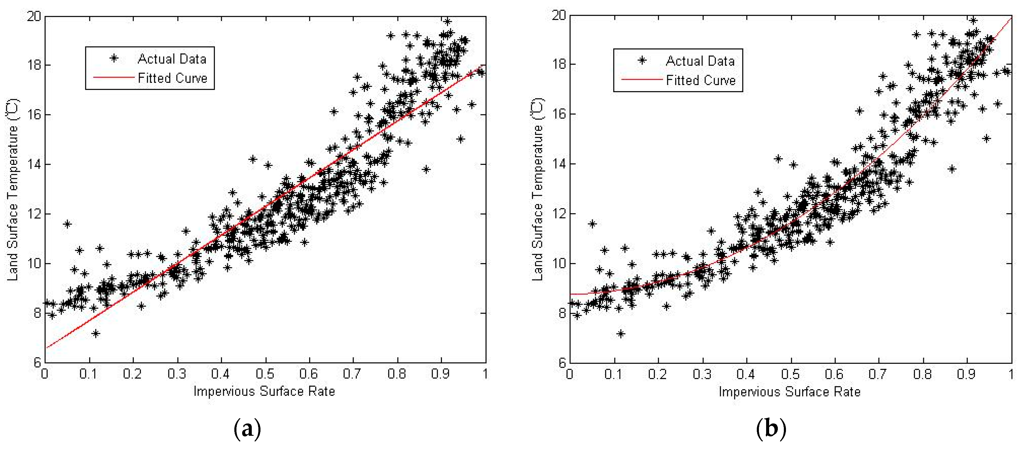
Figure 15.
Relationship between NDVI and LST.

Figure 16.
Relationship between NDVI and LST.

Table 1.
Climate data for Shanghai [36].
Table 1.
Climate data for Shanghai [36].
| Jan | Feb | Mar | Apr | May | Jun | Jul | Aug | Sep | Oct | Nov | Dec | |
|---|---|---|---|---|---|---|---|---|---|---|---|---|
| Avg Temp. (℃) | 4 | 5 | 8 | 14 | 19 | 24 | 28 | 27 | 23 | 18 | 12 | 7 |
| Wind Direction (°) | 290 | 40 | 0 | 110 | 90 | 110 | 150 | 140 | 60 | 20 | 20 | 290 |
| Wind Speed (m/s) | 2 | 3 | 3 | 3 | 3 | 2 | 4 | 2 | 3 | 2 | 3 | 2 |
| Relative Humidity | 73 | 78 | 73 | 76 | 81 | 83 | 79 | 77 | 82 | 75 | 73 | 70 |
| Global Horiz Radiation (Avg Daily Total, Wh/sq.m) | 2131 | 2362 | 2791 | 4041 | 4119 | 4003 | 4782 | 5061 | 3257 | 3338 | 2533 | 2316 |
| Avg precipitation (mm) | 74.4 | 59.1 | 93.8 | 74.2 | 84.5 | 181.8 | 145.7 | 213.7 | 87.1 | 55.6 | 52.3 | 43.9 |
Table 2.
Experimental data collection.
| File Name | 2002003 | 2007033 | 2013337 |
|---|---|---|---|
| Location | Shanghai | ||
| Sensor | Landsat5 TM | Landsat5 TM | Landsat8 OLI |
| Spatial | 30 × 30 m | ||
| Temporal | 3 January 2002 | 2 February 2007 | 3 December 2013 |
| Spectral (micrometers) | Band 1 = Blue (0.45–0.52) Band 2 = Green (0.52–0.6) Band 3 = Red (0.63–0.69) Band 4 = NIR (0.76–0.9) Band 5 = SWIR (1.55–1.75) Band 6 = TIR (10.4–12.5) * Band 7 = SWIR (2.08–2.35) | Band 1 = Blue (0.45–0.52) Band 2 = Green (0.52–0.6) Band 3 = Red (0.63–0.69) Band 4 = NIR (0.76–0.9) Band 5 = SWIR (1.55–1.75) Band 6 = TIR (10.4–12.5) * Band 7 = SWIR (2.08–2.35) | Band 1 = Coastal (0.433–0.453) Band 2 = Blue (0.450–0.515) Band 3 = Green (0.525–0.6) Band 4 = Red (0.630–0.680) Band 5 = NIR (0.845–0.885) Band 6 = SWIR 1 (1.560–1.660) Band 7 = SWIR 2 (2.100–2.300) Band 8 = Pan (0.500–0.680) * Band 9 = Cirrus (1.360–1.390) Band 10 = TIRS 1 (10.6–11.2) * Band 11 = TIRS 2 (12.0–12.5) * |
* The spatial resolutions of Pan, TIR and TIRS bands are 15 m, 120 m and 100 m respectively (Source: https://www.usgs.gov) [37].
Table 3.
Dynamic change of the impervious surface of Shanghai.
| Year | 2002 | 2009 | 2013 |
|---|---|---|---|
| Percentage | 19.47% | 36.23% | 37.09% |
| Area (km2) | 1234.40 | 2296.98 | 2351.56 |
Table 4.
Accuracy assessment of impervious surface extraction of Shanghai.
| Year | 2002 | 2009 | 2013 |
|---|---|---|---|
| Accuracy | 90.50% | 87.79% | 89.34% |
Table 5.
Land use classification accuracy.
| Year | 2002 | 2009 | 2013 |
|---|---|---|---|
| Overall Accuracy | 85.59% | 83.20% | 88.14% |
| Kappa Coefficient | 0.7874 | 0.7536 | 0.8117 |
Table 6.
The range of 7 land surface temperature intervals.
| Temperature Grade | Range |
|---|---|
| Extreme high temperature | |
| High temperature | |
| Sub-high temperature | |
| Medium temperature | |
| Sub-medium temperature | |
| Sub-low temperature | |
| Low temperature |
represents land surface temperature. is the average land surface temperature. is standard deviation.
Table 7.
Impervious surface statistics information data (km2).
| Downtown | Pudong | Minhang | Baoshan | Jiading | |
| 2002 | 160.87 | 217.63 | 126.59 | 148.41 | 86.71 |
| 2007 | 242.64 | 528.73 | 230.77 | 210.64 | 216.13 |
| 2013 | 238.95 | 544.71 | 231.06 | 216.39 | 216.70 |
| Jinshan | Songjiang | Qingpu | Fengxian | Chongming | |
| 2002 | 35.93 | 64.15 | 69.78 | 50.41 | 177.92 |
| 2007 | 111.27 | 165.76 | 155.06 | 194.93 | 241.05 |
| 2013 | 112.86 | 180.09 | 155.64 | 196.77 | 258.39 |
Table 8.
Regional proportion of impervious surface.
| Downtown | Pudong | Minhang | Baoshan | Jiading | |
| 2002 | 55.66% | 17.98% | 34.03% | 49.47% | 18.89% |
| 2007 | 83.95% | 43.69% | 62.03% | 70.21% | 47.08% |
| 2013 | 82.68% | 45.02% | 62.11% | 72.13% | 47.21% |
| Jinshan | Songjiang | Qingpu | Fengxian | Chongming | |
| 2002 | 6.13% | 10.60% | 10.32% | 7.34% | 15.01% |
| 2007 | 18.99% | 27.39% | 22.94% | 28.37% | 20.34% |
| 2013 | 19.26% | 29.76% | 23.02% | 28.64% | 21.80% |
Table 9.
Regional change of impervious surface (km2).
| Downtown | Pudong | Minhang | Baoshan | Jiading | |
| 2002–2007 | 81.77 | 311.10 | 104.18 | 62.23 | 129.42 |
| 2007–2013 | −3.69 | 15.98 | 0.29 | 5.75 | 0.57 |
| Total | 78.08 | 327.08 | 104.47 | 67.98 | 129.99 |
| Jinshan | Songjiang | Qingpu | Fengxian | Chongming | |
| 2002–2007 | 75.34 | 101.61 | 85.28 | 144.52 | 63.13 |
| 2007–2013 | 1.59 | 14.33 | 0.58 | 1.84 | 17.34 |
| Total | 76.93 | 115.94 | 85.86 | 146.36 | 80.47 |
Table 10.
Growth rate of impervious surface area.
| Downtown | Pudong | Minhang | Baoshan | Jiading | |
| 2002–2007 | 50.83% | 142.95% | 82.29% | 41.93% | 149.25% |
| 2007–2013 | −1.52% | 3.02% | 0.126% | 2.73% | 0.264% |
| Jinshan | Songjiang | Qingpu | Fengxian | Chongming | |
| 2002–2007 | 209.68% | 158.39% | 122.21% | 286.68% | 35.48% |
| 2007–2013 | 1.43% | 8.65% | 0.374% | 0.944% | 7.19% |
Table 11.
LUCC: Land-use and land-cover change (km2).
| Urban | Vegetation | Water | Other | |
|---|---|---|---|---|
| 2002 | 2105.96 | 2375.86 | 165.64 | 1692.84 |
| 2007 | 2940.93 | 1785.94 | 202.10 | 1413.76 |
| 2013 | 2562.84 | 1973.15 | 175.39 | 1629.98 |
Table 12.
Urban heat island intensive distribution in different dstricts (°C).
| 2002 Avg Temp. | 2002 UHI Intensity | 2007 Avg Temp. | 2007 UHI Intensity | 2013 Avg Temp. | 2013 UHI Intensity | |
|---|---|---|---|---|---|---|
| Jinshan | 7.697 | −0.586 | 10.736 | −0.806 | 10.436 | −0.753 |
| Qingpu | 7.459 | −0.824 | 10.908 | −0.638 | 9.974 | −1.246 |
| Songjiang | 8.084 | −0.274 | 10.813 | −0.742 | 11.942 | 0.764 |
| Minhang | 9.577 | 1.297 | 13.647 | 2.217 | 14.145 | 2.135 |
| Baoshan | 9.485 | 1.266 | 14.636 | 3.122 | 13.746 | 1.894 |
| Downtown | 12.192 | 3.978 | 16.135 | 4.914 | 15.864 | 4.217 |
| Pudong | 9.997 | 1.797 | 14.742 | 3.033 | 12.798 | 1.853 |
| Jiading | 9.096 | 0.897 | 14.126 | 2.783 | 13.120 | 1.935 |
| Fengxian | 7.437 | −0.721 | 11.063 | −0.523 | 11.752 | −0.004 |
| Chongming | 7.765 | −0.416 | 11.130 | −0.024 | 8.969 | −2.131 |
| Total | 8.846 | 1.463 | 11.837 | 2.012 | 11.033 | 1.894 |
© 2017 by the authors. Licensee MDPI, Basel, Switzerland. This article is an open access article distributed under the terms and conditions of the Creative Commons Attribution (CC BY) license (http://creativecommons.org/licenses/by/4.0/).
Share and Cite
MDPI and ACS Style
Wang, H.; Zhang, Y.; Tsou, J.Y.; Li, Y. Surface Urban Heat Island Analysis of Shanghai (China) Based on the Change of Land Use and Land Cover. Sustainability 2017, 9, 1538. https://doi.org/10.3390/su9091538
AMA Style
Wang H, Zhang Y, Tsou JY, Li Y. Surface Urban Heat Island Analysis of Shanghai (China) Based on the Change of Land Use and Land Cover. Sustainability. 2017; 9(9):1538. https://doi.org/10.3390/su9091538
Chicago/Turabian StyleWang, Haiting, Yuanzhi Zhang, Jin Yeu Tsou, and Yu Li. 2017. "Surface Urban Heat Island Analysis of Shanghai (China) Based on the Change of Land Use and Land Cover" Sustainability 9, no. 9: 1538. https://doi.org/10.3390/su9091538
Note that from the first issue of 2016, this journal uses article numbers instead of page numbers. See further details here.