Rapid Detection of Land Cover Changes Using Crowdsourced Geographic Information: A Case Study of Beijing, China


College of Geography and Environment, Shandong Normal University, Jinan 250300, Shandong, China
*
Author to whom correspondence should be addressed.
Sustainability 2017, 9(9), 1547; https://doi.org/10.3390/su9091547
Submission received: 1 July 2017
/
Revised: 24 August 2017
/
Accepted: 26 August 2017
/
Published: 30 August 2017
Abstract
:Land cover change (LCC) detection is a significant component of sustainability research including ecological economics and climate change. Due to the rapid variability of natural environment, effective LCC detection is required to capture sufficient change-related information. Although such information has been available through remotely sensed images, the complicated image processing and classification make it time consuming and labour intensive. In contrast, the freely available crowdsourced geographic information (CGI) contains easily interpreted textual information, and thus has the potential to be applied for capturing effective change-related information. Therefore, this paper presents and evaluates a method using CGI for rapid LCC detection. As a case study, Beijing is chosen as the study area, and CGI is applied to monitor LCC information. As one kind of CGI which is generated from commercial Internet maps, points of interest (POIs) with detailed textual information are utilised to detect land cover in 2016. Those POIs are first classified into land cover nomenclature based on their textual information. Then, a kernel density approach is proposed to effectively generate land cover regions in 2016. Finally, with GlobeLand30 in 2010 as baseline map, LCC is detected using the post-classification method in the period of 2010–2016 in Beijing. The result shows that an accuracy of 89.20% is achieved with land cover regions generated by POIs, indicating that POIs are reliable for rapid LCC detection. Additionally, an LCC detection comparison is proposed between remotely sensed images and CGI, revealing the advantages of POIs in terms of LCC efficiency. However, due to the uneven distribution, remotely sensed images are still required in areas with few POIs.
1. Introduction
Land cover change (LCC) refers to the dynamics of biophysical materials covering the earth surface [1], and it has emerged as a fundamental component of sustainability research [2], including ecological economics, climate change, etc. [3,4]. In the past few years, numerous LCC products have been developed using remotely sensed images [5]. In general, these are often detected through the classification of multi-temporal remote sensing images, using post-classification approaches or direct radiometric comparison approaches [6]. However, the time and labour costs could be quite expensive due to the complexities of LCC detection [7,8], and these are crucial factors to determine the development of sustainability [9]. This has further simulated intensive research for rapid LCC detection with lower time and labour costs.
The increasing availability of crowdsourced geographic information (CGI) has drawn the attention of researchers as a source of up-to-date and freely available data for LCC detection. CGI, which is crowdsourced data with coordinate information, is generated from users on the Internet, and usually contains textual information corresponding to land cover classes [10]. CGI is usually available through geoweb-based tagging systems to facilitate LCC detection, where geo-tagged data are encouraged to be uploaded by volunteers via mobile devices, such as OpenStreetMap (OSM) [11,12,13,14]. It has been considered as training data of remotely sensed images [15], or provided socioeconomic features in urban regions detection with the combination of satellite data in rural regions [16]. However, these approaches rely on the acquisition and classification of remotely sensed images with considerable labour and time cost. This inspired further investigation to employ CGI for changes detection to complement the shortcoming of remote sensing. A recent research study proposed a method of generating up-to-date maps using textual information from OSM [17,18]. Since these kinds of data were provided by volunteers, textual information is often insufficient and incomplete for rapid LCC detection.
The shortcoming of volunteer-generated data necessitates the need of CGI with detailed textual information. In general, this CGI often exists in commercial Internet maps, such as Google Maps, Baidu Maps, and Gaode Maps. Such maps contain sufficient information about land cover classes, which is aggregated as points of interest (POIs) [19]. These POIs are provided with up-to-date data, and are usually updated on a timely basis to capture land cover changes. Furthermore, POIs are usually freely available via Application Programming Interfaces (APIs). The API is usually offered by commercial Internet mapping companies, which also ensure the quality of these POIs. Therefore, there is strong potential to employ such high quality CGI for rapid LCC detection. In this study, we propose an approach for rapid LCC detection by utilising POIs from commercial Internet maps. First, textual information from POIs are converted into land cover nomenclature. Then, we apply kernel density to generate land cover regions represented by POIs. Finally, a post-classification approach is proposed for rapid LCC detection. A comparative experiment using remotely sensed images is also proposed to compare both labour and time cost for LCC detection.
2. Experimental Data and Study Area
In this paper, Beijing, which is located in the north of China, is used as the study area. Containing a total area of 16,410.54 km2 (the area lies between 39°26′–41°03′N and 115°25′–117°30′E), Beijing includes artificial surfaces, forest, grassland, and cultivated land as dominant land cover classes in this area, accompanied with other various classes such as water bodies, wetland, and shrubland. The land cover in Beijing experienced significant changes due to rapid urbanization. The above consequences led to great complexity of land cover changes in a short period of time and are great barriers to LCC production. While detecting land cover changes with remotely sensed images is time consuming, CGI can be interpreted effectively to necessitate the need of land cover detection.
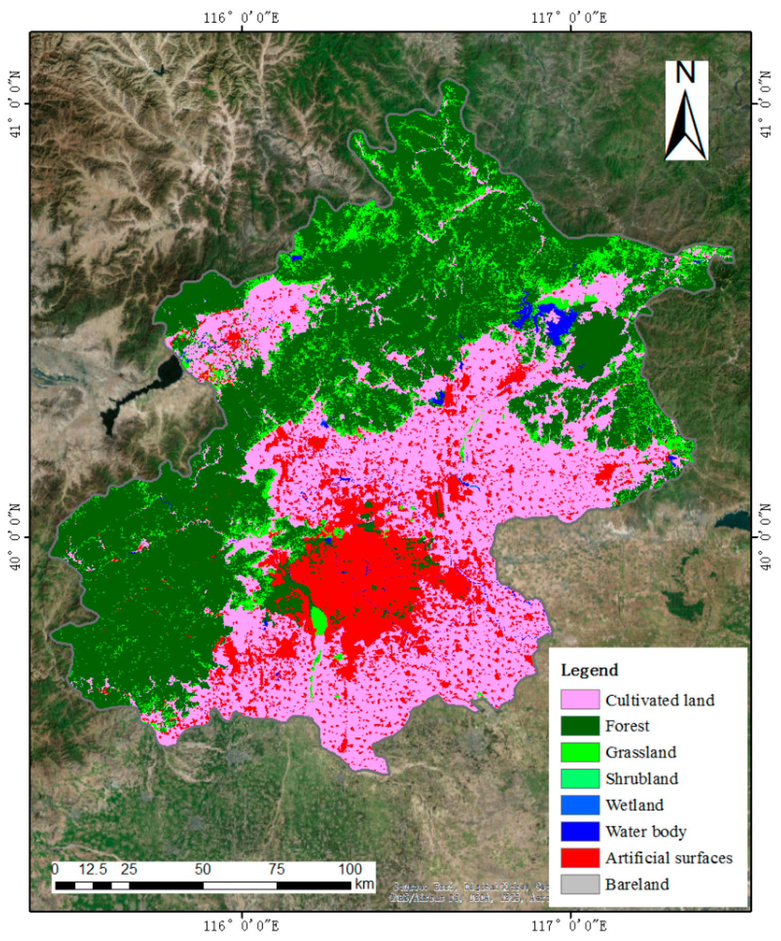
We chose GlobeLand30 with 30 m × 30 m resolution in 2010 as the baseline map for change detection. GlobeLand30, which is produced by the National Geomatic Center of China (NGCC), is one of the first global 30 m land cover products [20]. Land cover products for the year of 2000 and 2010 were created with 10 land cover classes including cultivated land, forest, grassland, shrubland, wetland, water bodies, tundra, artificial surfaces, bare land, and permanent snow/ice. The distribution of land cover classes of GlobeLand30 in 2010 in Beijing is shown Figure 1. Furthermore, an overall classification accuracy of over 80% has been achieved via land cover validation [21]. Thus, GlobeLand30 in 2010 was chosen in our study as reference data of 2010.
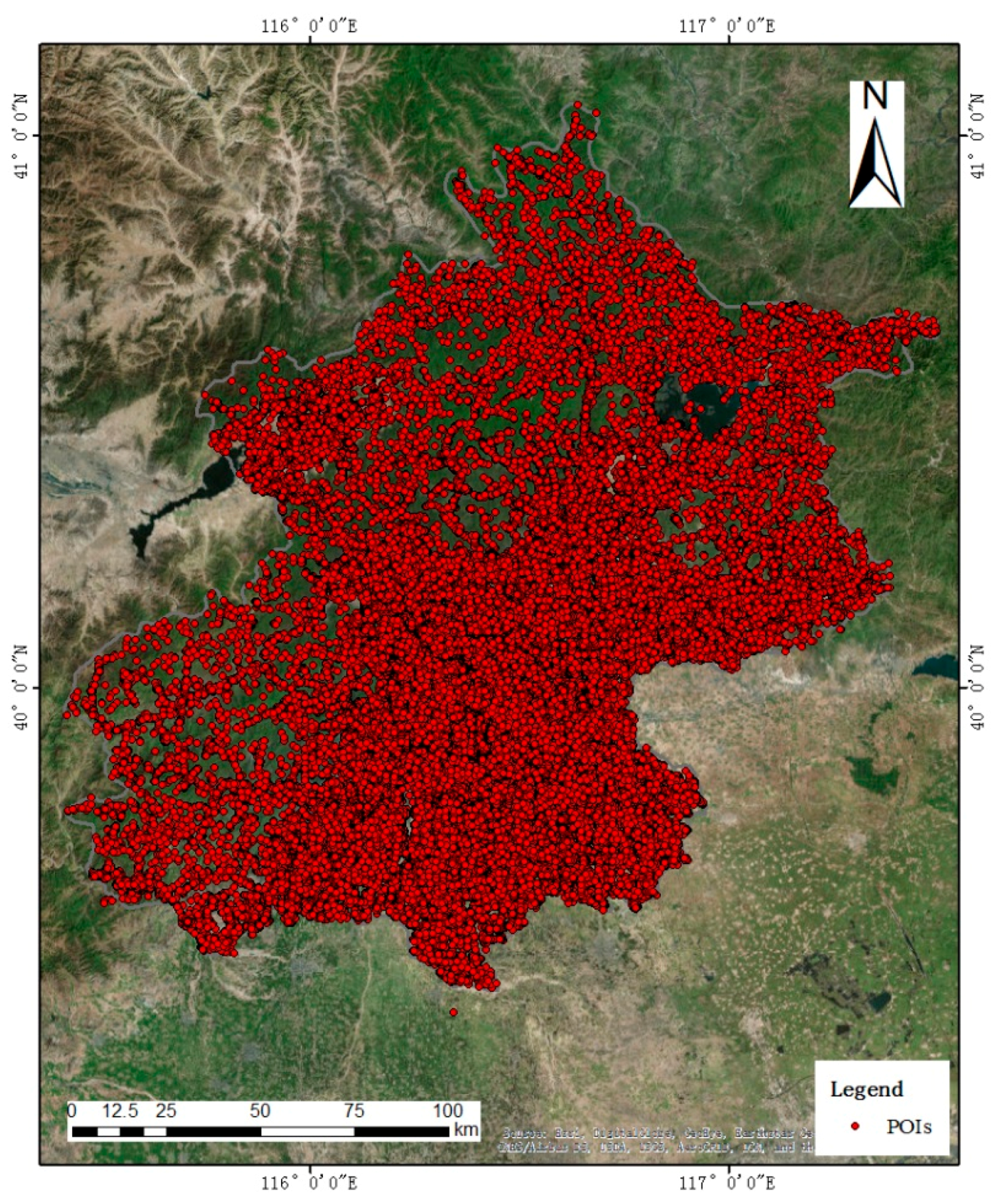
In terms of POIs, a total number of 1,528,104 POIs in 2016 were obtained from Gaode map, a commercial Internet map in China (Figure 2). These data were collected through API offered by AutoNavi in “http://lbs.amap.com/getting-started/search”. The POIs include information such as coordinate positions, the names of locations, the POI types, and other detailed information. For the purpose of detecting land cover classes of POIs, we collected the land cover related information including POI coordinate positions and POI types. Although the names of POIs offer a lot of detailed evidence about the located places, such as “Walmart” as POI name and “supermarket” as POI type, the latter is sufficient enough to represent land cover classes, as we can conduce easily that “supermarket” belongs to artificial surfaces. Furthermore, as the names of POIs are usually different from one another, classifying a huge amount of POIs is relatively labour intensive. Therefore, we consider the types of POIs to indicate land cover classes and for further land cover classification. The veracity of this textual information in POIs is evaluated by selecting randomly and interpreting 200 sites where POIs are located. The result shows that most sites are labelled with the correct POIs, except three sites corresponding to the wrong POI types. Despite the existence of a few mislabelled POIs, a large quantity of POIs is still valuable to represent correct places.
3. Methodology
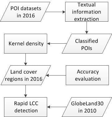
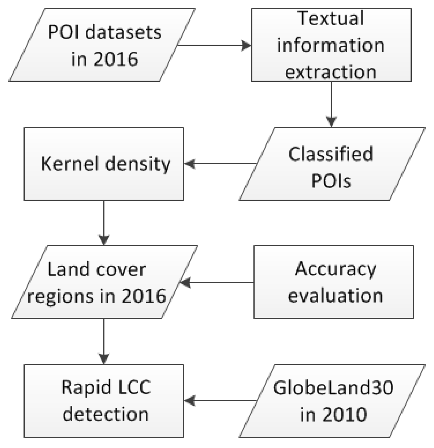
The methodology of rapid LCC detection using POIs is shown in Figure 3. First, POIs in 2016 are utilised to identify current land cover classes. Since POIs contain detailed textual information, we extract the information as a clue to correspond to land cover classes. Thus, POIs are classified into different nomenclature of GlobeLand30. Details are explained in Section 3.1. Then, we use classified POIs to generate land cover regions in 2016 using kernel density, followed by combining Globeland30 in 2010 to detect LCC in the 2010–2016 period. This step is explained in detail in Section 3.2. Third, to evaluate the accuracy of land cover regions in 2016 generated by POIs, we apply a confusion matrix to assess the result of each land cover class. This step is discussed in Section 3.3.
3.1. POIs Classification
Detecting land cover changes requires up-to-date land cover classes generated by POIs. To apply POIs for classifying land cover, textual information in POI types is extracted to be classified in different land cover classes based on the nomenclature in GlobeLand30. Part of the classified POIs is shown in Table 1. Most of the POIs are classified as cultivated land, forest/grassland, water bodies, and artificial surfaces. It should be noted that grassland and forest are mixed into one land cover class because of the relatively small numbers of POIs in both land cover classes. The remaining POIs cannot be classified into certain land cover classes, such as “Agriculture, forestry, animal husbandry, and fishery base”, which indicates a wide range of land cover including cultivated land, forest, grassland, and water bodies. Thus, these POI types are excluded from our study.
To ensure POI classification accuracy, a random sampling is proposed to validate the land cover class that each POI is classified into. We select a total number of 200 POIs randomly, in which 50 POIs are chosen in cultivated land, forest/grassland, water bodies, and artificial surfaces, respectively. After interpreting each site manually, the classification accuracy of the POIs is shown in Table 2. The overall accuracy of POI classification is around 81% among these land cover classes. The accuracy of POIs that are classified as water bodies is relatively low, because many POIs related to water bodies are actually located beside them. To eliminate the above classification error, this paper reconsiders the land cover changes that are from other classes to water bodies. The details are shown in Section 4.3.
3.2. Land Cover Region Generation and Change Detection
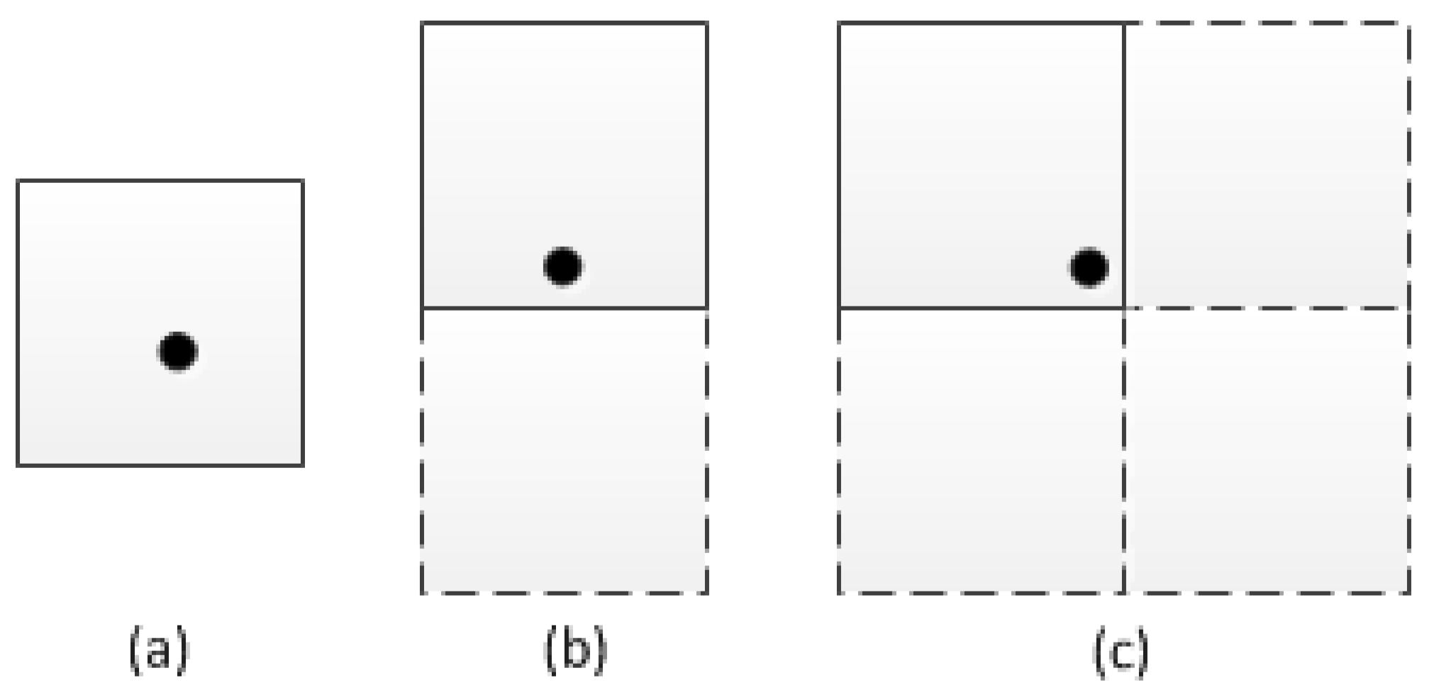
Rapid LCC detection requires land cover comparison between the baseline map (GlobeLand30 in 2010) and land cover regions in 2016. As the classified POIs in Section 3.1 are simply points that are located in the 30 m × 30 m grid (the same resolution as GlobeLand30) when comparing the differences with GlobeLand30, generating land cover regions from POIs remains a problem that needs to be solved first. Figure 4 displays the probable POI locations when overlaying on the 30 m × 30 m grid. In Figure 4a, POI is located around the centre of the grid, and the areas that this POI represents can be within the regions of this grid. However, the POI in Figure 4b,c distributes near the edge and the corner of the located grid (see the grids in solid line), separately, which leads to great potential that the neighbouring grids (see the grids in dotted line) may also contain land cover classes shared by the located POI. Therefore, the areas represented by each POI can be included within approximately a radius of 30 m.
Taking the above consequences into consideration, an area estimation method is required to generate land cover regions that are generated from POIs. As an effective way to estimate the density of a random variable, kernel density [22] is able to converse independent points into continuous areas with a proper radius of influence. Previous studies have applied kernel density in identifying facility hotspots [23], flood assessment [24], delineating urban-rural boundary [25], and other applications. However, few studies utilise it to generate land cover regions. Therefore, we utilise kernel density to estimate areas of each land cover class according to the classified POIs in Table 1. The equation of kernel density is shown as follows:
where h represents the bandwidth of the kernel density, determining the generated areas of POIs. We set the bandwidth as 30 m according to the analysis of POI location in Figure 4. n indicates the number of POIs that are within the distance of bandwidth h. is the kernel function that is applied in kernel density. x represents the POI that is to be estimated, and represents the surrounding POIs with in bandwidth. The values of the kernel density are represented in the resolution of 30 m × 30 m. While the calculated value changes with different densities, areas where the density is larger than 0 are extracted as land cover regions that POIs represented. Part of the generated land cover regions is shown in Figure 5. As the POIs in these areas are classified as artificial surfaces, we apply kernel density with the bandwidth of 30 m and generate continuous land cover regions of artificial surfaces.
After regions of each land cover nomenclature are generated from POIs using kernel density, these generated regions can be overlapped in the areas that feature a high density of POIs. Table 3 summarises the overlapping conditions of regions generated by POIs. Group 1 represents land cover regions that are not overlapped, including cultivated land, forest/grassland, water bodies, and artificial surfaces. These regions are the readily identified areas and can be used directly in detecting land cover regions. Group 2 includes overlapped land cover regions that are mixed by cultivated land, forest/grassland, and water bodies. These regions can hardly be classified into a single land cover class without other reference data. To ensure the land cover changes accuracy, we move out these regions from group 2. On the other hand, group 3 represents areas which contain artificial surfaces and other land cover classes. As each kind of mixed region includes artificial surfaces, we converge all of these regions into artificial surfaces. The reason is that artificial surfaces are usually related to human activities, and it is relatively complex because artificial surfaces often contain public facilities related to water bodies or other land cover classes. The land cover regions generated by POIs with a certain class can be seen in Figure 6 in Section 4.1.
For LCC detection, both the baseline map in 2010 and land cover regions generated by POIs in 2016 are overlaid to identify changes by proposing the post-classification method, and all land cover transitions can be detected during the 2010–2016 period. However, it should be noted that as we group forest and grassland into a single land cover category, any areas that show conversions from forest to forest/grassland or from grassland to forest/grassland are considered as unchanged areas.
3.3. Accuracy Evaluation
To validate land cover regions generated from POIs, a random stratified sampling is proposed as reference data with 50 points for the classes of cultivated land, forest/grassland, and water bodies, and 100 points for artificial surfaces, which is the dominant land cover class in Beijing. More reference points in artificial surfaces are collected because artificial surfaces take up the largest areas in the generated land cover regions in 2016 (see details in Section 4.1). These 250 reference data are classified through visual interpretation based on remotely sensed images on Google Earth. Then, a confusion matrix is created by comparing generated land cover regions in 2016 and reference points. Both the producer’s accuracy and user’s accuracy can be calculated to assess classification accuracy for each land cover class. Moreover, an overall accuracy is applied to evaluate land cover classification of all classes.
4. Results
4.1. Land Cover Regions Deriving from POIs
Land cover classification results of POIs are shown in Table 4. One million five hundred eleven thousand, three hundred and eight (1,511,308) of a total 1,528,104 POIs are considered as artificial surfaces, occupying 98.90% of all POIs. Water bodies contain 2496 POIs, which only covers 0.16% of total POIs. Cultivated land and forest/grassland contain 1830 and 815 POIs, relatively, with the proportion of 0.11% and 0.05% of total POI number. The remaining 11,655 POIs are unclassified, taking up 0.76% of all POIs. This indicates that the largest proportion of POIs belongs to artificial surfaces. Further, POIs corresponding to non-artificial surfaces (namely cultivated land, forest/grassland, water bodies, and unclassified class) take up only no more than 2% of all data.
Based on the POI classification in Table 3, land cover regions are generated from POIs, and the results are shown in Figure 6. Most of the areas belong to artificial surfaces, which is consistent with the proportion of POIs classified as the same class. For the regions of cultivated land, forest/grassland, and water bodies, they occupied much smaller proportions of areas because of the relatively low number of POIs.
A detailed analysis is displayed in Table 5 In total, 96,128.28 ha were generated from the classified POIs, with 1,068,092 grids (each grid was 30 m × 30 m). Among these land cover classes, artificial surfaces occupy the largest areas, with 95,035.5 ha, which take up 98.86% of the total 96,128.28 ha area. Five thousand nine hundred and seventy-three (5973) grids are classified as water bodies with areas of 537.57 ha, about 0.56% of all areas. Only 4089 grids refer to cultivated land, which occupies 368.01 ha in total generated areas. Forest/grassland takes up the smallest areas and totals 187.2 ha with the percentage of 0.19%.
4.2. Accuracy Evaluation
Table 6 shows the confusion matrix between land cover regions generated from POIs and reference points. The result indicates that an overall accuracy of 89.20% is achieved in this area. In terms of producer’s accuracy (PA), a value of 94.23% is achieved in the artificial surfaces class. The accuracy of cultivated land and forest/grassland are 80.36% and 81.48%, respectively. As for the class of water bodies, the user’s accuracy (UA) is much lower, with the value of 72.00%, while the value 100% is achieved in producer’s accuracy. Visual inspection of the low user’s accuracy in water bodies show that several points are actually located in cultivated land and forest/grassland, and a few of them are distributed in artificial surfaces. Forest/grassland shows a user’s accuracy of 88.00%, which is much higher than that of producer’s accuracy. Cultivated land and artificial surfaces achieved an UA value of 90.00% and 98.00%, respectively, with an increasing value of approximately 10% and 4% compared with producer’s accuracy.
In general, the classification accuracy in Table 6 indicates that the land cover regions in 2016 generated from POIs are reliable in the application of land cover changes detection. It is worth noting that the user’s accuracy of water bodies is relatively low. Therefore, future work will investigate other land cover classification approaches in order to improve the classification accuracy. Further, the classification of Globeland30 in 2010 shows an accuracy of approximately 80% [21]. Based on the above analysis, it shows that GlobeLand30 and regions generated from POIs can be used to detect land cover changes from 2010 to 2016.
4.3. Rapid LCC Detection Using POIs
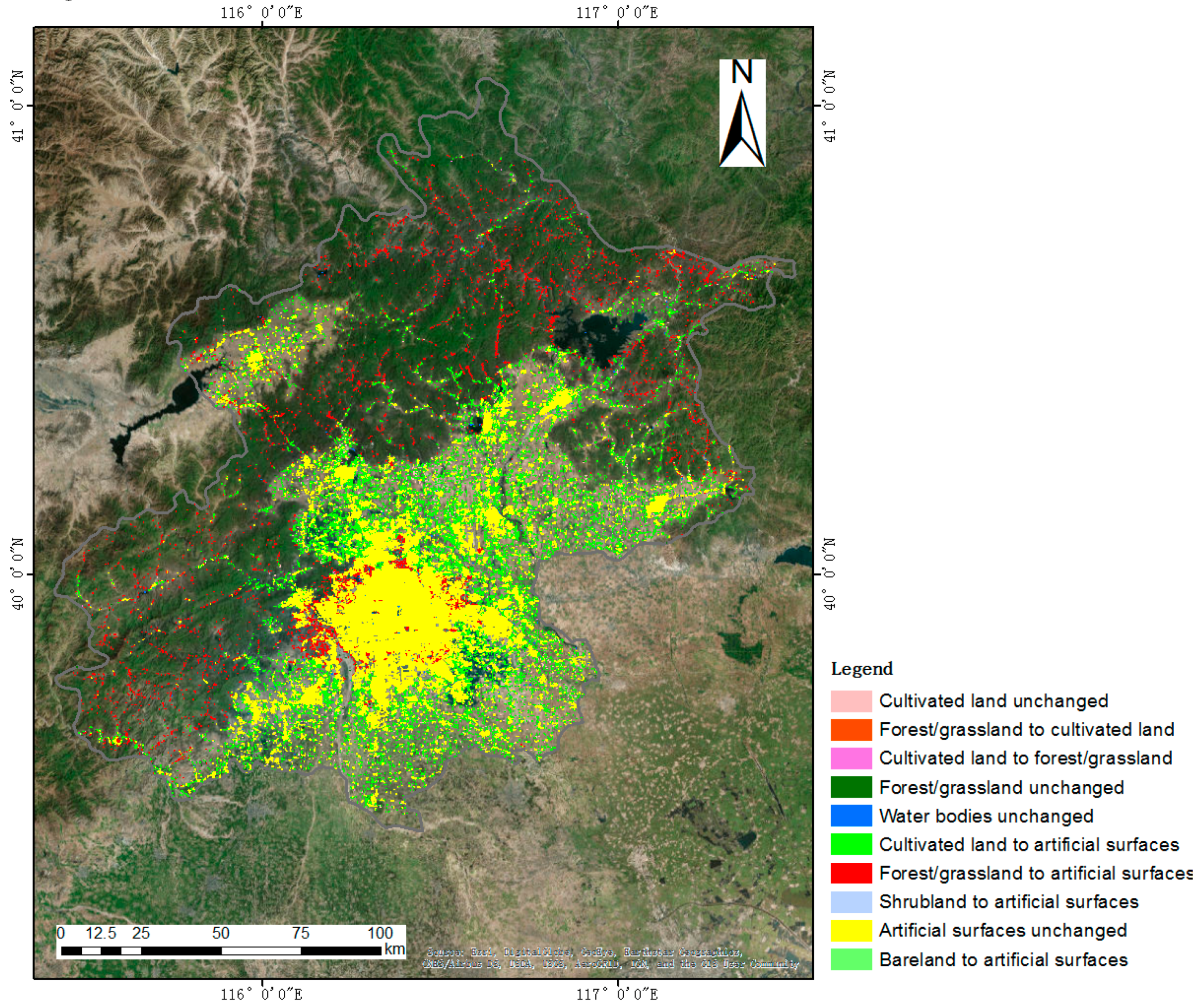
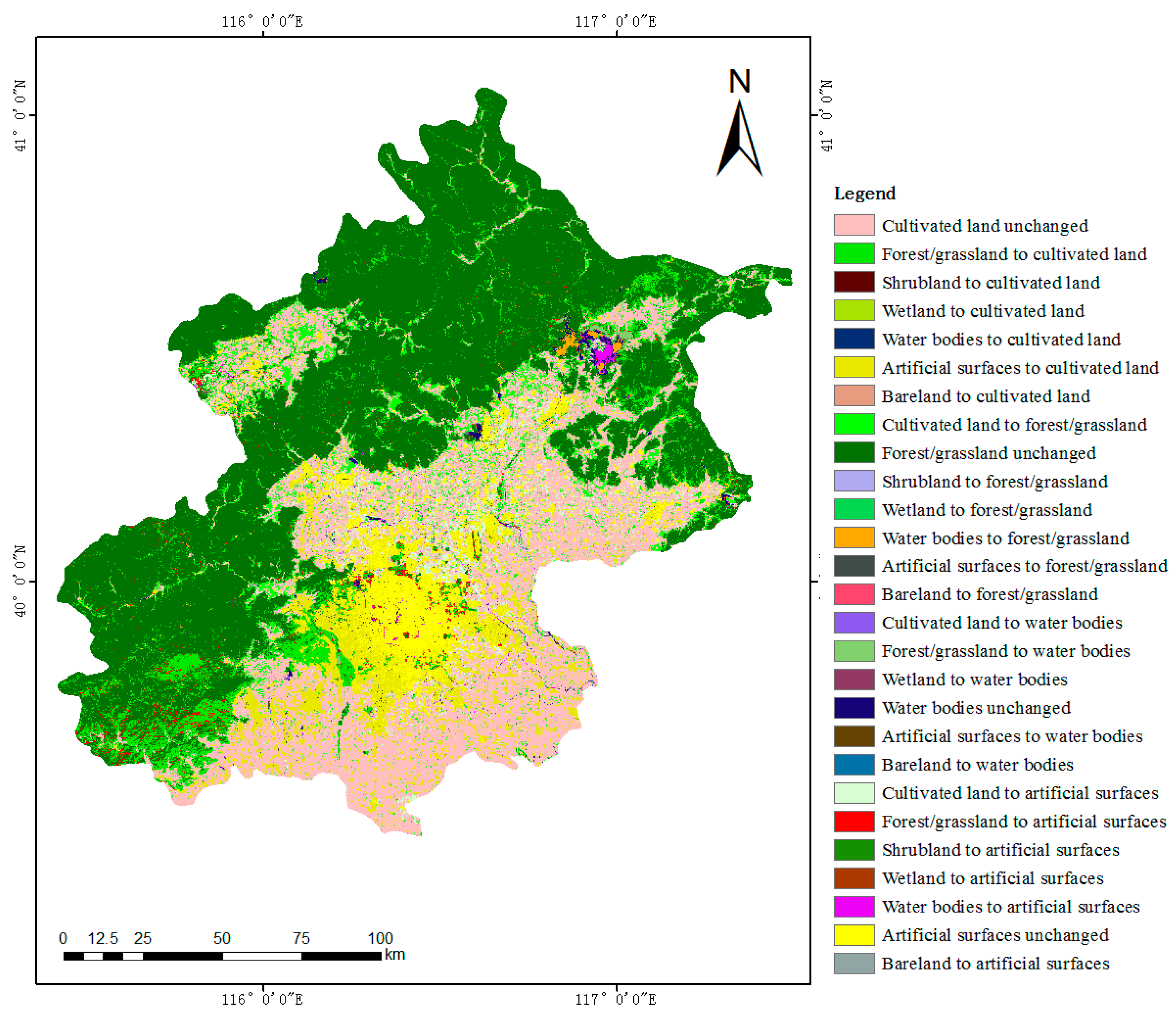
We proposed a post-classification method with land cover regions generated by POIs in 2016 and GlobeLand30 in 2010. Based on the POIs classification and the corresponding land cover regions above, four kinds of unchanged land cover classes and 18 kinds of changed classes were detected during this period. However, since the POI classification accuracy of water bodies in Table 2 is relatively low, LCC that is from other land cover classes to water bodies is considered as the unchanged original land cover. On the other hand, LCC that is from artificial surfaces or water bodies to other land cover classes is regarded as unchanged artificial surfaces. This is due to the fact that artificial surfaces and water bodies are not likely to be transitioned to other classes. Moreover, as Table 5 indicates that cultivated land, forest/grassland, and water bodies only collectively contain a small proportion of areas, they are less able to be fully used in LCC detection. As a result, four kinds of unchanged classes and six kinds of changed classes are represented in Figure 7. Changes from forest/grassland to cultivated land, cultivated land to forest/grassland, cultivated land to artificial surfaces, forest/grassland to artificial surfaces, shrubland to artificial surfaces, and bareland to artificial surfaces are detected in this area. For a visual overview of land cover changes in Beijing, artificial surfaces remain the largest areas among four unchanged classes. Other unchanged classes including cultivated land, forest/grassland, and water bodies only occupy a small proportion of the total areas. Both LCC from cultivated land and forest/grassland to artificial surfaces have a high percentage increase among the changed land cover regions, while other changes occupy fewer regions due to the limited number of POIs.
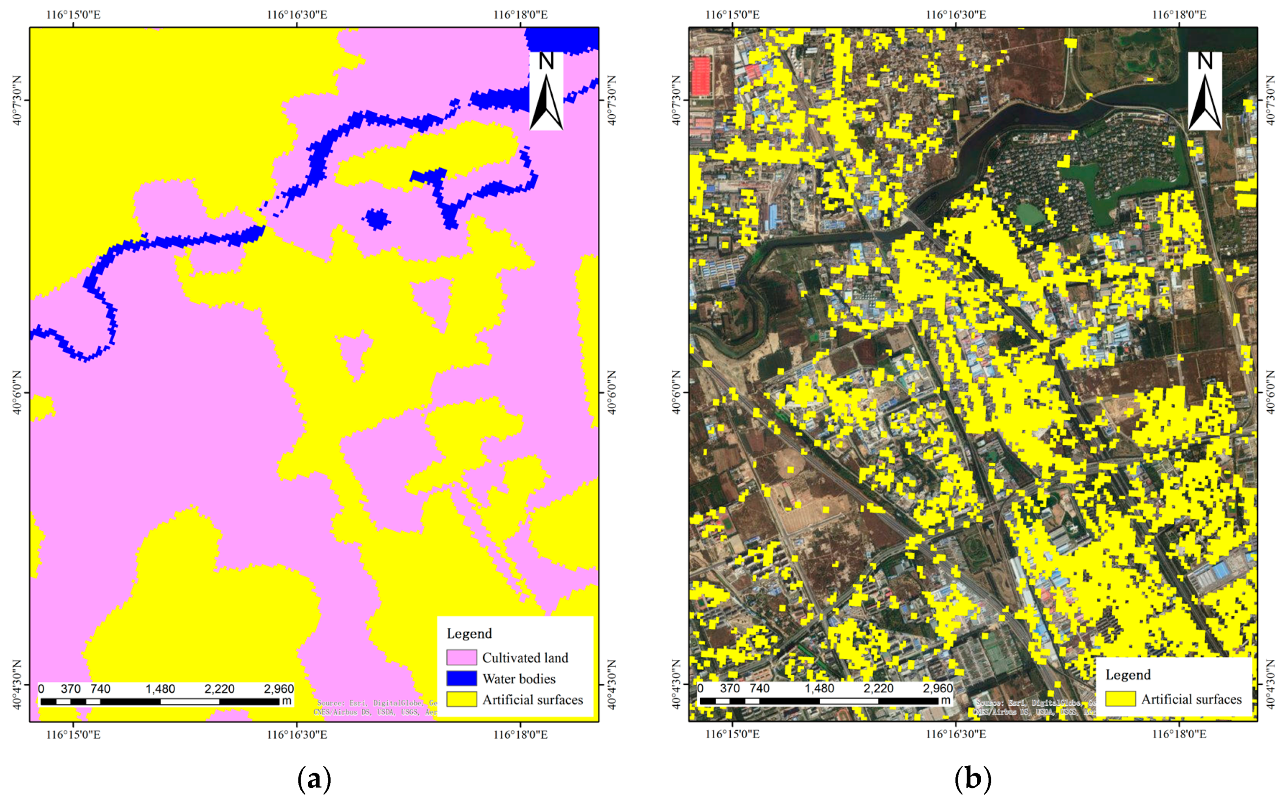
In detail, LCC can be shown in both rural and urban regions. Figure 8 displays land cover transition from cultivated land to artificial surfaces in rural regions. Areas in yellow represent artificial surfaces. Compared with the artificial surfaces in 2010 in Figure 8a, areas in 2016 in Figure 8b have a much wider distribution. This indicates that a large number of areas of cultivated land are replaced by artificial surfaces in the period of 2010 to 2016. We highlight these changes in Figure 8c with green areas. These changes can be validated visually by referring to the images provided by Esri, one of which is shown in Figure 8d. This shows that an expansion of built-up areas replace cultivated land during this period.
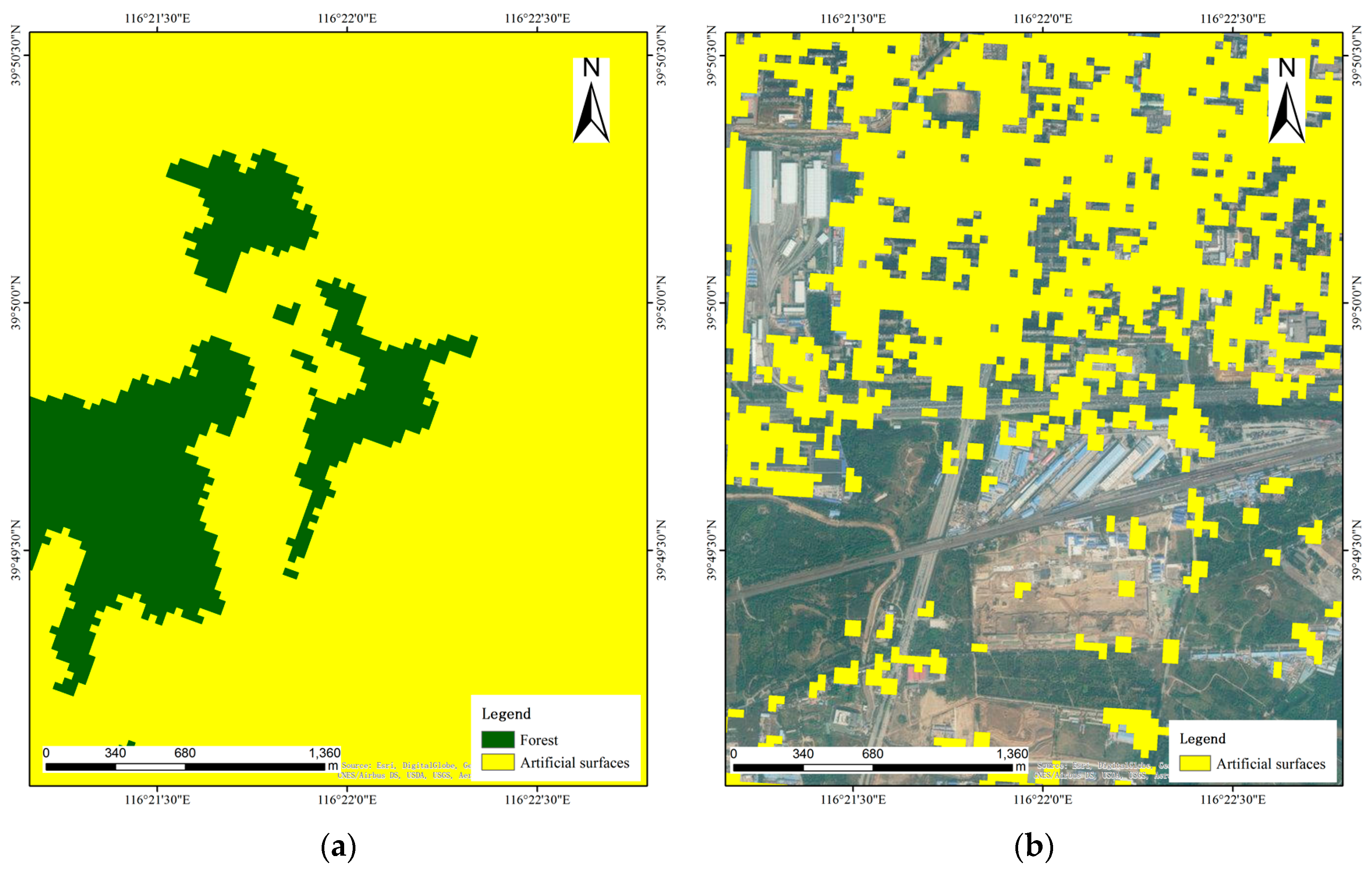
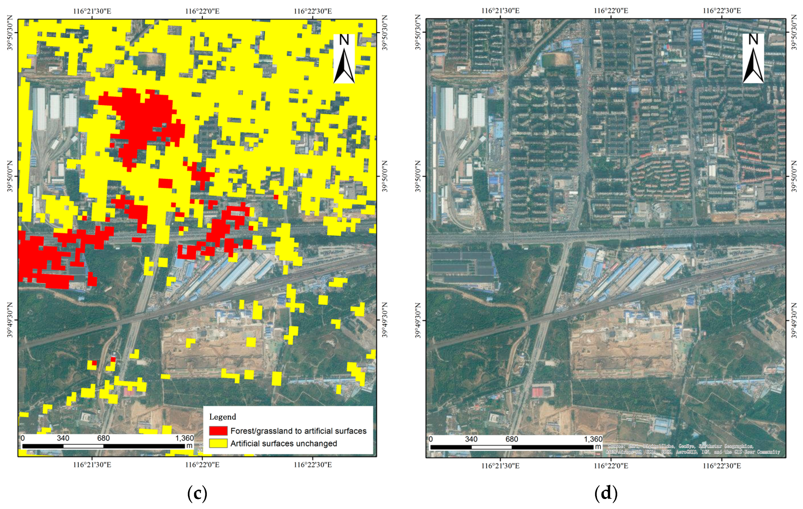
LCC can also be detected in urban areas, where land cover transitions from forest/grassland to artificial surfaces (Figure 9). Figure 9a,b display the changes of artificial surfaces and forest/grassland in the period of 2010 to 2016. An increase of artificial surfaces can be seen in the north and west of the area, although the land cover regions generated by POIs are sparser because of the lack of POIs (Figure 9c). These changes are highlighted in red in Figure 9c, which can be evaluated based on images in Figure 9d.
4.4. LCC Detection Comparison between Remotely Sensed Images and CGI
To compare the LCC detection efficiency between POIs and remotely sensed images, a traditional method is proposed to monitor LCC in the 2010–2016 period. In general, LCC detection usually contains two methods, namely post-classification approaches and direct radiometric comparison approaches. LCC detection with post-classification approaches is based on the comparison of land cover classification using remotely sensed images, while direct radiometric comparison approaches propose a comparison of images before classifying land cover. Noting that we use the GlobeLand30 product as land cover in 2010 and do not rely on remotely sensed images, we use post-classification approaches for LCC detection.
We selected three images from Landsat 8 in 2016 as experimental data. Since these images are not generated in the same time, the atmospheric conditions can be variable. Therefore, both radiometric calibration and atmospheric correction are required for data pre-processing. Then, we used Maximum likelihood classifier to classify land cover with the processed images. As training data are required via image interpretation, we selected eight data samples as water bodies, twenty-five data samples as forest/grassland, thirty data samples as cultivated land, and thirty-two data samples as artificial surfaces. On the other hand, CGI usually contains land cover information and does not rely on selecting training data via image interpretation. After images from Landsat 8 were classified with different land cover classes, a post-classification approach was applied to detect LCC using classified regions and GlobeLand30 in 2010. The result is shown in Figure 10. Since land cover regions generated by Landsat 8 data are much wider than POIs, the LCC transitions are more complicated with different land cover classes.
Then, we analysed the differences and efficiency of these two data sources. The methods comparison is displayed in Table 7. In the stage of data pre-processing, both remotely sensed images and CGI are processed to extract useful land cover information. However, pre-processing with remotely sensed images is very time consuming, as radiometric calibration, atmospheric correction, and image mosaic are very complicated. More importantly, the increasing number of remotely sensed images could extend this pre-processing routine. Taking the experiment above as an example, three images from Landsat 8 covering Beijing are processed within two hours. In contrast, unclassified CGI can be easily extracted based on their textual information. For instance, processing POIs according to their categories was completed within 10 min in the study. Such POI pre-processing cannot be more complex due to the standard categories of POIs.
In terms of data classification, conventional methods require training data for each class. To complement this process, image interpretation is required by selecting several regions for each class from remotely sensed images. In this study, a total number of sixty-five training data were randomly selected in the area of Beijing, and it took approximately two hours for one volunteer to confirm the actual land cover classes of each training data. On the other hand, we group POIs into different classes according to their categories. This process takes about less than half an hour, since ambiguous POI categories have been removed in the pre-processing stage. Furthermore, the POI classification process would not be extended when detecting LCC in much wider regions, while image classification indeed requires considerable time to select more training data.
Land cover regions generation/classification using remotely sensed images and CGI are both utilised by automatic methods, with the formal using Maximum likelihood classifier, Decision tree classifier, etc. and the latter using kernel density and overlapping rules. In this study, we classified Landsat 8 data using Maximum likelihood classifier, and it took about fifteen minutes to complete the process. Although it is much more effective than data pre-processing and classification, the generation of land cover regions with POIs only takes a few seconds to automatically complete the entire area.
In the last stage, changes are extracted by comparing up-to-date land cover regions with the baseline map. Since land cover regions have been generated by both remotely sensed images and CGI, the efficiency of this stage is quite similar, with approximately fifteen minutes required for either process.
5. Conclusions and Future Work
In this study, we employed POIs from commercial Internet maps for rapid LCC detection. Taking Beijing as study area, POIs in 2016 were selected to represent land cover currently, and GlobeLand30 with the resolution of 30 m × 30 m was applied to offer detailed land cover information in 2010. To generate land cover regions of 2016, POIs were classified into different land cover classes based on their textual information. Then, kernel density was utilised to estimate the regions of different land cover classes. In order to find proper bandwidth in kernel density, we analysed the different positions of 30 m × 30 m grids that POIs can locate. Furthermore, the overlapping regions that were generated from POIs were analysed to determine the final land cover class. Finally, a post-classification method was proposed using land cover regions generated from POIs and GlobeLand30 in 2010 to detect LCC in Beijing in the period of 2010–2016. The overall accuracy of land cover regions generated from POIs was 89.20%, suggesting the usability of POIs in terms of LCC detection. Additionally, LCC detection efficiency was compared between remotely sensed images and POIs, indicating the reliability of rapid LCC detection using POIs.
In spite of the rapid LCC detection we proposed, several questions are still beyond consideration and will be solved in future work, which are listed below as follows:
- (1)
- Due to the spatial heterogeneity of POIs [26], most POIs are located in artificial surfaces. This limits the application of the proposed method to some extent. However, as POIs are often generated because of human activities, which are usually the main reason behind rapid land cover changes, it is possible to utilise POIs to monitor land cover changes effectively. Further, considering that commercial Internet maps contain more types of data except for POIs, there are possibilities to extract sufficient information corresponding to various land cover classes. Furthermore, due to the uneven distribution, remotely sensed images are still required in areas with few POIs.
- (2)
- When generating land cover regions, we defined a radius of 30 meters in kernel density based on the resolution of GlobeLand30. However, the land cover regions generated by POIs can be various, due to the diversity of textual information in POIs [19]. For example, a POI representing “golf course” refers to much larger areas than a POI representing “shop”. One solution may be to focus on selecting the proper parameter of radius in kernel density. Each kind of POI is set by a typical weight when determining the radius of land cover regions. In that case, POIs named “golf course” will be given a larger weight of radius before being applied to kernel density. Based on this consideration, we will investigate more effective approaches considering both CGI textual information and spatial distributions in future work.
- (3)
- Considering the uneven proportion of land cover regions which are generated by POIs, it is not appropriate that all classes should be applied for LCC detection. Therefore, this study analyses the LCC result in Section 4.3, and considers several LCC as invalid transitions. However, as our proposed method is not limited to utilising POIs, multi-sourced data including commercial Internet maps and OpenStreetMap can also be utilised to fill the gap between the uneven distribution of POIs and continuous land cover regions.
- (4)
- Since most POIs are simply classified as artificial surfaces, detailed information that is related to human activities is ignored, such as land use information [27]. For example, POIs with “Restaurant” and ”Apartment” categories represent commercial areas and residential areas, respectively. Future works would consider CGI for land use changes detection by applying the textual information in CGI.
Acknowledgments
This research was supported by the National Natural Science Foundation of China (Grant No. 41501420, 41701443), and China Postdoctoral Science Foundation Funded Project (Grant No. 2017M612330, 2017M612329).
Author Contributions
Yuan Meng implemented the method, performed the major part of experiments, and drafted the manuscript. Dongyang Hou made substantial contributions to the conceptual design and methodological development. Hanfa Xing developed the framework and wrote the manuscript.
Conflicts of Interest
The authors declare no conflict of interest.
References
- Chen, J.; Li, S.; Wu, H.; Chen, X. Towards a collaborative global land cover information service. Int. J. Digit. Earth 2017, 10, 356–370. [Google Scholar] [CrossRef]
- Turner, B.L.; Lambin, E.F.; Reenberg, A. The emergence of land change science for global environmental change and sustainability. Proc. Natl. Acad. Sci. USA 2007, 104, 20666–20671. [Google Scholar] [CrossRef] [PubMed]
- Hadorn, G.H.; Bradley, D.; Pohl, C.; Rist, S.; Wiesmann, U. Implications of transdisciplinarity for sustainability research. Ecol. Econ. 2006, 60, 119–128. [Google Scholar] [CrossRef]
- Stock, P.; Burton, R.J. Defining terms for integrated (multi-inter-trans-disciplinary) sustainability research. Sustainabity 2011, 3, 1090–1113. [Google Scholar] [CrossRef] [Green Version]
- Chen, X.; Chen, J.; Shi, Y.; Yamaguchi, Y. An automated approach for updating land cover maps based on integrated change detection and classification methods. ISPRS J. Photogram. Remote Sens. 2012, 71, 86–95. [Google Scholar] [CrossRef]
- Chen, J.; Lu, M.; Chen, X.; Chen, J.; Chen, L. A spectral gradient difference based approach for land cover change detection. ISPRS J. Photogram. Remote Sens. 2013, 85, 1–12. [Google Scholar] [CrossRef]
- Fonte, C.C.; Bastin, L.; See, L.; Foody, G.; Lupia, F. Usability of VGI for validation of land cover maps. Int. J. Geogr. Inf. Sci. 2015, 29, 1269–1291. [Google Scholar] [CrossRef]
- Hou, D.; Chen, J.; Wu, H.; Li, S.; Chen, F.; Zhang, W. Active collection of land cover sample data from geo-tagged web texts. Remote Sens. 2015, 7, 5805–5827. [Google Scholar] [CrossRef]
- Hernandez, M. A digital earth platform for sustainability. Int. J. Digit. Earth 2017, 10, 342–355. [Google Scholar] [CrossRef]
- Liu, Y.; Liu, X.; Gao, S.; Gong, L.; Kang, C.; Zhi, Y.; Chi, G.; Shi, L. Social sensing: A new approach to understanding our socioeconomic environments. Ann. Assoc. Am. Geogr. 2015, 105, 512–530. [Google Scholar] [CrossRef]
- Xing, H.; Chen, J.; Zhou, X. A geoweb-based tagging system for borderlands data acquisition. ISPRS Int. J. Geo-Inf. 2015, 4, 1530–1548. [Google Scholar] [CrossRef]
- Fritz, S.; McCallum, I.; Schill, C.; Perger, C.; See, L.; Schepaschenko, D.; Van der Velde, M.; Kraxner, F.; Obersteiner, M. Geo-wiki: An online platform for improving global land cover. Environ. Model. Softw. 2012, 31, 110–123. [Google Scholar] [CrossRef]
- Han, G.; Chen, J.; He, C.; Li, S.; Wu, H.; Liao, A.; Peng, S. A web-based system for supporting global land cover data production. ISPRS J. Photogram. Remote Sens. 2015, 103, 66–80. [Google Scholar] [CrossRef]
- Estima, J.; Painho, M. Investigating the potential of openstreetmap for land use/land cover production: A case study for continental Portugal. In Openstreetmap in Giscience; Springer: Berlin, Germany, 2015; pp. 273–293. [Google Scholar]
- Johnson, B.A.; Iizuka, K.; Bragais, M.A.; Endo, I.; Magcale-Macandog, D.B. Employing crowdsourced geographic data and multi-temporal/multi-sensor satellite imagery to monitor land cover change: A case study in an urbanizing region of the philippines. Comput. Environ. Urban Syst. 2017, 64, 184–193. [Google Scholar] [CrossRef]
- Hu, T.; Yang, J.; Li, X.; Gong, P. Mapping urban land use by using landsat images and open social data. Remote Sens. 2016, 8, 151. [Google Scholar] [CrossRef]
- Fonte, C.C.; Minghini, M.; Patriarca, J.; Antoniou, V.; See, L.; Skopeliti, A. Generating up-to-date and detailed land use and land cover maps using openstreetmap and globeland30. ISPRS Int. J. Geo-Inf. 2017, 6, 125. [Google Scholar] [CrossRef]
- Fonte, C.C.; Patriarca, J.; Minghini, M.; Antoniou, V.; See, L.; Brovelli, M.A. Using openstreetmap to create land use and land cover maps: Development of an application. Volunt. Geogr. Inf. Future Geosp. Data 2017, 113–137. [Google Scholar]
- Xing, H.; Meng, Y.; Hou, D.; Song, J.; Xu, H. Employing crowdsourced geographic information to classify land cover with spatial clustering and topic model. Remote Sens. 2017, 9, 602. [Google Scholar] [CrossRef]
- Chen, J.; Ban, Y.; Li, S. China: Open access to earth land-cover map. Nature 2014, 514, 434. [Google Scholar]
- Chen, J.; Chen, J.; Liao, A.; Cao, X.; Chen, L.; Chen, X.; He, C.; Han, G.; Peng, S.; Lu, M. Global land cover mapping at 30m resolution: A pok-based operational approach. ISPRS J. Photogram. Remote Sens. 2015, 103, 7–27. [Google Scholar] [CrossRef]
- Rosenblatt, M. Remarks on some nonparametric estimates of a density function. Ann. Math. Stat. 1956, 27, 832–837. [Google Scholar] [CrossRef]
- Hart, T.; Zandbergen, P. Kernel density estimation and hotspot mapping: Examining the influence of interpolation method, grid cell size, and bandwidth on crime forecasting. Polic. Intern. J. Police Strateg. Manag. 2014, 37, 305–323. [Google Scholar] [CrossRef]
- Schnebele, E. Improving remote sensing flood assessment using volunteered geographical data. Nat. Hazard. Earth Syst. Sci. 2013, 13, 669. [Google Scholar] [CrossRef]
- Peng, J.; Zhao, S.; Liu, Y.; Tian, L. Identifying the urban-rural fringe using wavelet transform and kernel density estimation: A case study in beijing city, china. Environ. Model. Soft. 2016, 83, 286–302. [Google Scholar] [CrossRef]
- Xing, H.; Meng, Y.; Hou, D.; Cao, F.; Xu, H. Exploring point-of-interest data from social media for artificial surface validation with decision trees. Inter. J. Remote Sens. 2017, 38, 6945–6969. [Google Scholar] [CrossRef]
- Frias-Martinez, V.; Frias-Martinez, E. Spectral clustering for sensing urban land use using twitter activity. Eng. Appl. Artif. Intell. 2014, 35, 237–245. [Google Scholar] [CrossRef]
Figure 1.
GlobeLand30 in 2010 in Beijing with eight land cover classes.

Figure 2.
Point of interest (POI) distributions in Beijing.

Figure 3.
The workflow of methodology. LCC, land cover change.

Figure 4.
POI location in different position of grids. (a) POIs around the centre of the located grid. (b) POIs near the edge of the located grid. (c) POIs near the corner of the located grid.
Figure 4.
POI location in different position of grids. (a) POIs around the centre of the located grid. (b) POIs near the edge of the located grid. (c) POIs near the corner of the located grid.

Figure 5.
Part of the land cover regions of artificial surfaces from POIs.
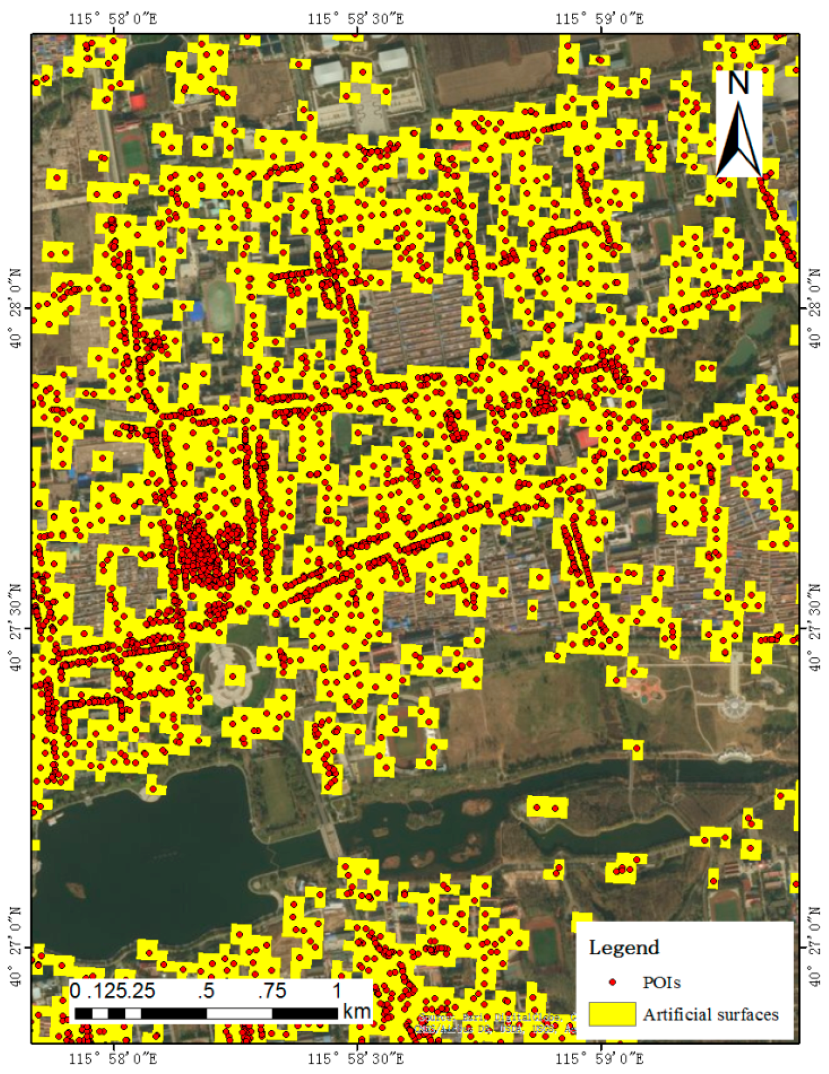
Figure 6.
Land cover regions generated from POIs in Beijing.
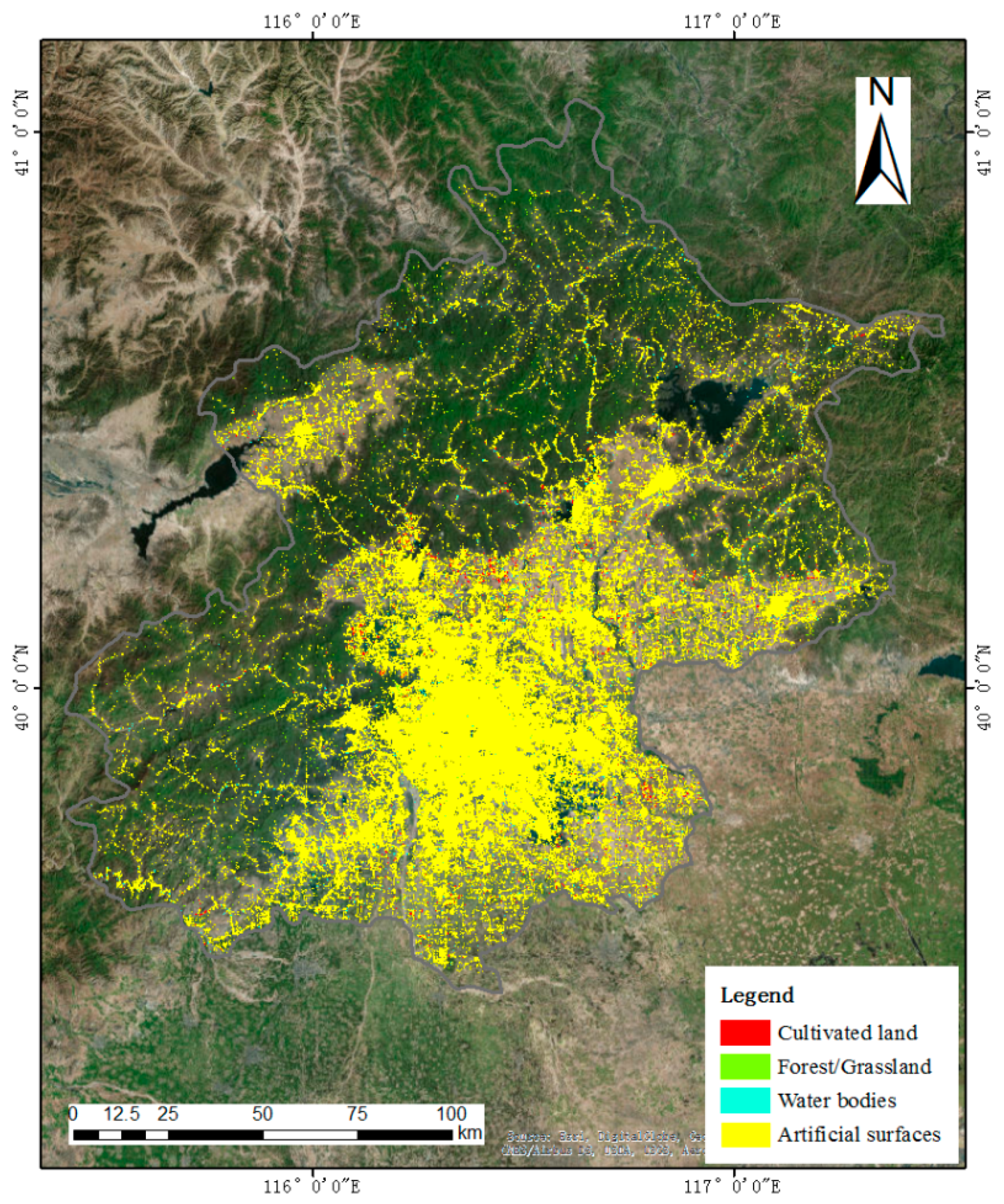
Figure 7.
Land cover changes in the period of 2010 to 2016.

Figure 8.
Subset of land cover transition from cultivated land to artificial surfaces in the period of 2010 to 2016. (a) Land cover regions of GlobeLand30 in 2010; (b) Land cover regions generated from POIs in 2016; (c) LCC from 2010 to 2016; (d) Remotely sensed image provided by Esri.
Figure 8.
Subset of land cover transition from cultivated land to artificial surfaces in the period of 2010 to 2016. (a) Land cover regions of GlobeLand30 in 2010; (b) Land cover regions generated from POIs in 2016; (c) LCC from 2010 to 2016; (d) Remotely sensed image provided by Esri.

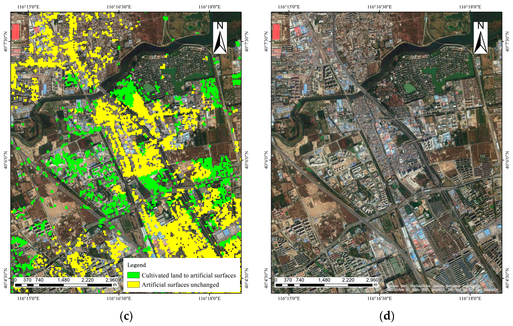
Figure 9.
Subset of land cover transition from forest/grassland to artificial surfaces in the period of 2010 to 2016. (a) Land cover regions of GlobeLand30 in 2010; (b) Land cover regions generated from POIs in 2016; (c) LCC from 2010 to 2016; (d) Remotely sensed image provided by Esri.
Figure 9.
Subset of land cover transition from forest/grassland to artificial surfaces in the period of 2010 to 2016. (a) Land cover regions of GlobeLand30 in 2010; (b) Land cover regions generated from POIs in 2016; (c) LCC from 2010 to 2016; (d) Remotely sensed image provided by Esri.


Figure 10.
LCC using Landsat 8 data in the 2010–2016 period.


Table 1.
Land cover nomenclature corresponding to POI types.
| Land Cover Nomenclature | POI Types |
|---|---|
| Cultivated land | Vegetable base, Fruit base, Farmland, Nursery garden, etc. |
| Forest/Grassland | Golf course, Golf practice field, Mountain, Botanical garden, Pasture, etc. |
| Water bodies | Fishing park, Port, Pier, Beach, River, Lake, Bridge, Ferry, etc. |
| Artificial surfaces | Restaurant, Supermarket, Residential area, School, Library, etc. |
| Unclassified class | Agriculture, Forestry, Animal husbandry, and Fishery base, Leisure place, etc. |
Table 2.
POI classification accuracy.
| Land Cover Class | CL | FG | WB | AS | Total |
|---|---|---|---|---|---|
| Cultivated land (CL) | 43 | 6 | 0 | 1 | 50 |
| Forest/Grassland (FG) | 3 | 41 | 0 | 6 | 50 |
| Water bodies (WB) | 6 | 9 | 30 | 5 | 50 |
| Artificial surfaces (AS) | 1 | 1 | 0 | 48 | 50 |
| Total | 53 | 57 | 30 | 60 | 200 |
| Accuracy | 81% |
Table 3.
Overlapping conditions of land cover regions generated from POIs.
| Group 1 | Group 2 | Group 3 |
|---|---|---|
| Cultivated land | Cultivated land + Forest/Grassland | Artificial surfaces + Cultivated land |
| Forest/Grassland | Cultivated land + Water bodies | Artificial surfaces + Forest/Grassland |
| Water bodies | Forest/Grassland + Water bodies | Artificial surfaces + Water bodies |
| Artificial surfaces | Artificial surfaces + Cultivated land + Forest/Grassland | |
| Artificial surfaces + Cultivated land + Water bodies | ||
| Artificial surfaces + Forest/Grassland + Water bodies |
Table 4.
Numbers and proportions of POIs in each land cover class.
| Land Cover Class | Number of POI | Percentage (%) |
|---|---|---|
| Cultivated land | 1830 | 0.11% |
| Forest/grassland | 815 | 0.05% |
| Water bodies | 2496 | 0.16% |
| Artificial surfaces | 1,511,308 | 98.90% |
| Unclassified class | 11,655 | 0.76% |
| Total | 1,528,104 | 100% |
Table 5.
Classes of land cover regions in 2016 with the number of grids, areas, and the percentage of total areas.
Table 5.
Classes of land cover regions in 2016 with the number of grids, areas, and the percentage of total areas.
| Land Cover Class | Number of Grids | Areas/ha | Percentage (%) |
|---|---|---|---|
| Cultivated land | 4089 | 368.01 | 0.38% |
| Forest/Grassland | 2080 | 187.2 | 0.19% |
| Water bodies | 5973 | 537.57 | 0.56% |
| Artificial surfaces | 1,055,950 | 95,035.5 | 98.86% |
| Total | 1,068,092 | 96,128.28 | 100.00% |
Table 6.
Classification results for the land cover regions in 2016. (PA for producer’s accuracy, UA for user’s accuracy).
Table 6.
Classification results for the land cover regions in 2016. (PA for producer’s accuracy, UA for user’s accuracy).
| Land Cover Class | CL | FG | WB | AS | Total | UA (%) |
|---|---|---|---|---|---|---|
| Cultivated land (CL) | 45 | 5 | 0 | 0 | 50 | 90.00% |
| Forest/Grassland (FG) | 3 | 44 | 0 | 3 | 50 | 88.00% |
| Water bodies (WB) | 6 | 5 | 36 | 3 | 50 | 72.00% |
| Artificial surfaces (AS) | 2 | 0 | 0 | 98 | 100 | 98.00% |
| Total | 56 | 54 | 36 | 104 | 250 | |
| PA (%) | 80.36% | 81.48% | 100.00% | 94.23% | 89.20% |
Table 7.
Methods comparison of LCC detection between crowdsourced geographic information (CGI) remotely sensed images and CGI.
Table 7.
Methods comparison of LCC detection between crowdsourced geographic information (CGI) remotely sensed images and CGI.
| Remotely Sensed Images | CGI | |
|---|---|---|
| Data pre-processing | Requiring radiometric calibration, atmospheric correction, image mosaic etc. | Extracting unclassified CGI based on their textual information. |
| Data classification | Selecting training data of each class by interpreting images. | Classifying CGI based on their textual information. |
| Land cover regions generation/classification | Auto-classification by Maximum likelihood classifier, Decision tree classifier etc. | Generating land cover regions by kernel density and overlapping rules. |
| Land cover changes detection | Post-classification by comparing land cover classification between land cover products and remotely sensed images | Post-classification by comparing land cover classification between POIs and land cover products. |
© 2017 by the authors. Licensee MDPI, Basel, Switzerland. This article is an open access article distributed under the terms and conditions of the Creative Commons Attribution (CC BY) license (http://creativecommons.org/licenses/by/4.0/).
Share and Cite
MDPI and ACS Style
Meng, Y.; Hou, D.; Xing, H. Rapid Detection of Land Cover Changes Using Crowdsourced Geographic Information: A Case Study of Beijing, China. Sustainability 2017, 9, 1547. https://doi.org/10.3390/su9091547
AMA Style
Meng Y, Hou D, Xing H. Rapid Detection of Land Cover Changes Using Crowdsourced Geographic Information: A Case Study of Beijing, China. Sustainability. 2017; 9(9):1547. https://doi.org/10.3390/su9091547
Chicago/Turabian StyleMeng, Yuan, Dongyang Hou, and Hanfa Xing. 2017. "Rapid Detection of Land Cover Changes Using Crowdsourced Geographic Information: A Case Study of Beijing, China" Sustainability 9, no. 9: 1547. https://doi.org/10.3390/su9091547
Note that from the first issue of 2016, this journal uses article numbers instead of page numbers. See further details here.