Applying the Mahalanobis–Taguchi System to Improve Tablet PC Production Processes
by
 ,
,
Chi-Feng Peng
2,†, 
Li-Hsing Ho
3,†,
Sang-Bing Tsai
1,4,*,†,
Yin-Cheng Hsiao
3,
Yuming Zhai
5,*,
Quan Chen
1,*,
Li-Chung Chang
1 and
Zhiwen Shang
6,* 1
Zhongshan Institute, University of Electronic Science and Technology of China, Zhongshan 528402, China
2
Ph.D. Program of Technology Management, Chung Hua University, Hsinchu 300, Taiwan
3
Department of Technology Management, Chung-Hua University, Hsinchu 300, Taiwan
4
Economics and Management College, Civil Aviation University of China, Tianjin 300300, China
5
School of Economics and Management, Shanghai Institute of Technology, Shanghai 201418, China
6
Business School, Nankai University, Tianjin 300071, China
*
Authors to whom correspondence should be addressed.
†
These authors contributed equally to this work.
Sustainability 2017, 9(9), 1557; https://doi.org/10.3390/su9091557
Submission received: 25 July 2017
/
Revised: 25 August 2017
/
Accepted: 29 August 2017
/
Published: 1 September 2017
(This article belongs to the Special Issue Sustainability in Manufacturing)
Abstract
:Product testing is a critical step in tablet PC manufacturing processes. Purchases of testing equipment and on-site testing personnel increase overall manufacturing costs. In addition, to improve manufacturing capabilities, manufacturers must also produce products with higher quality and at a lower cost than their competitors if they are to attract consumers and gain a competitive edge in their industry. The Mahalanobis–Taguchi System (MTS) is a novel technique proposed by Genichi Taguchi for performing diagnoses and forecasting with multivariate data. The MTS can be used to select important factors and has been applied in numerous engineering fields to improve product and process quality. In the present study, the MTS, logistic regression, and a neural network were used to improve the tablet PC product testing process. The results indicated that the MTS attained 98% predictive power after insignificant test items were eliminated. The MTS performance was superior to those of the conventional logistic regression and neural network, which attained 93.3% and 94.7% predictive power, respectively. After the testing process was improved using the MTS, the number of test items in the tablet PC product testing process was reduced from 56 to 14. This facilitated the development of more stable test site configurations and effectively reduced the testing time, number of testers required, and equipment costs.
1. Introduction
The rapid development of cloud technology and changes in the computer usage habits of consumers and digital-oriented lifestyles have raised various discussions on the digital technology industry. In 2010, Apple Inc. (CA, USA) released its first tablet PC: the iPad. This began a global tablet boom that resulted in a gradual shrinking of the notebook market, which the tablet PC market is soon predicted to surpass in size. Manufacturers have increased their production capacity in response to this new market demand. An NPD (National Purchase Diary) DisplaySearch report stated that 256 million, 321 million and 350 million tablet PCs were shipped globally in 2014, 2015 and 2016, respectively [1]. The actual number of tablet PCs shipped in 2016 was more than the number of notebooks [2], as illustrated in Figure 1. Numerous PC manufacturers are concerned that tablet PCs are changing technology usage habits and what computer equipment consumers buy; furthermore, tablet PCs are expected to replace notebooks in the future.
The desire to enter the competitive tablet PC market has motivated major technology companies, such as Apple, Samsung, ASUS, ACER, HP, Dell and Amazon, to launch products that can derive a competitive advantage. These international brands have established operations worldwide, through which they can reach customers and satisfy their needs. Manufacturing, design, global logistics management, purchasing and other low-margin processes have gradually shifted to original equipment manufacturers (OEMs), with the brand companies instead focusing on marketing, which adds considerable value and is crucial for obtaining a competitive edge. This has substantially changed the methods with which OEMs conduct business. The demand of the global consumer market for tablet PCs is increasing daily, and the tablet PC industry is becoming increasingly sophisticated. Thus, this industry is becoming a perfectly competitive market. For the producers of standard PCs, the threshold to becoming a tablet PC OEM is low. Taiwan has advantages in this regard because of its PC production since the 1990s, and, consequently, most OEM work is performed locally [3]. Tablet PCs comprise aspects of traditional computers, notebooks, and mobile phones. They have distinct development processes and relatively short lifecycles with rapid product refresh rates [4]. Therefore, shortening product development times while maintaining quality standards is a critical concern in the technology industry.
Competition is intense in the tablet PC OEM industry. Manufacturers must continually improve their production capabilities and manufacture products with higher quality and at a lower cost than their competitors in order to attract consumers and derive a competitive advantage. Reducing production costs is thus a critical priority.
Product testing is an extremely crucial step in the tablet PC manufacturing process, but the procurement of testing equipment and the number of on-site testing personnel increase the overall manufacturing cost. In this study, the Mahalanobis–Taguchi System (MTS) was employed to improve tablet PC product-testing processes. Data were collected and analyzed, and scientific verification methods were employed to elucidate the product characteristics and construct meaningful models [5,6,7,8]. After the rationality of the tablet PC product testing items was evaluated, those that made small contributions were removed to facilitate accurate and rapid product testing. Thus, the number of test sites and testers was reduced, which decreased the testing costs, shortened the testing times, and enabled products to be release to the market more quickly. This strengthened company competitiveness within the industry as a whole. In addition, logistic regression and neural networks were used to improve the tablet PC product testing process. The differences among these three methods were subsequently compared and discussed.
2. Literature Review
2.1. Tablet PC Testing Process
The required test items are entirely different for each stage of the testing process. Tablet PC production test process includes PT1 (Pre-Test station 1) → PT2 → PT3 → PT4 → RIT (Run-in Test) → FT (Final Test) → QA (Quality Assurance) Check (Figure 2). At the production testing stage, tablet PCs are tested through production verification, functional testing, run-in, and volume production testing. Functional testing in particular accounts for a substantial portion of the overall production time. Therefore, functional testing was primarily investigated and improved in this study.
Currently, functional testing is extremely complex and certain content is repeated during both early and final testing. In addition, when faults occur during functional testing, the few devices analyzed and repaired during early testing are re-identified as faulty during the final testing. The MTS, logistic regression, and neural networks were employed in this study to identify more reasonable test items. High-quality engineering practices and professional engineering background knowledge were used to identify suitable test items while ensuring identical production quality [9,10].
2.2. MTS
The MTS is a classification technology devised by Dr. Genichi Taguchi for conducting diagnoses and forecasting with multivariate data [11,12]. It combines quality engineering principles and utilizes the Mahalanobis distance for the structured induction of data, serving as a basis for decision-making [13].
Mahalanobis space is established using k characteristic variables (X1, X2, …, Xk) derived from n normal products. It is used to distinguish normal products and abnormal products. The Mahalanobis distance calculated using a normal sample population has a mean approaching 1 and forms Mahalanobis space, which is also called base space. Mahalanobis space can be considered a database that includes characteristic variable means, standard deviations, and correlation coefficient inverse matrices for the normal population. Generally, the Mahalanobis distances of normal samples are less than 2.5, with values over 4 being extremely rare [14]. The Mahalanobis distance of a product from an abnormal sample that is calculated using the means, standard deviations, and correlation coefficient inverse matrices of base space is extremely high. Additionally, thresholds can be determined using the smallest type-I error (normal products misjudged as abnormal products) and type-II errors (abnormal products misjudged as normal products) that occur [15,16].
In robust design, targets in orthogonal arrays are used to minimize the number of tests. This minimal test number is used to obtain reliable factor effect estimates. In the MTS, orthogonal arrays verify useful variables using the minimal number of tests [17,18]. Within an orthogonal array, each characteristic variable or factor is placed in a different row. Each row is a combination of different variables or factor levels representing a test combination. By using orthogonal arrays, the influence of each characteristic variable on system output can be investigated [19,20]. A multivariate system was assumed to have k characteristic variables, and each characteristic variable was set to one of two levels:
- Level 1 = used characteristic variable; and
- Level 2 = unused characteristic variable.
The case analyzed in this study had 56 characteristic variables (X1–X56) that were used for analysis. Therefore, an L64(263) orthogonal array with an experimental configuration. Subsequently, the Mahalanobis space established by all of the characteristic variables in the normal sample was used to calculate the Mahalanobis distance of d abnormal samples (Equations (1)–(3)). This Mahalanobis distance was then used to obtain the signal-to-noise (SN) ratio [21,22].
Standardized equation:
where
Correlation matrix:
Inverse correlation matrix:
Mahalanobis distance:
After constructing the Mahalanobis space based on the characteristic variable combinations in the orthogonal array, the SN ratio were used to select important variables. In quality engineering, the SN ratio is used as an evaluation tool with decibels as a unit. The SN ratio is used to evaluate performance using the ratio of useful information to harmful information. In multivariate analysis, confirming that a combination of variables can fully detect abnormal levels is critical.
In this study, the level of abnormality in faulty tablet PCs was tested to serve as a basis for screening test items. The larger-the-better SN ratio was used in expectation that greater Mahalanobis distances within the abnormal sample observations in relation to those of the normal sample were favorable (Equation (4)).
Assuming that greater increases in Mahalanobis distances (average SN ratio of level 1 minus average SN ratio of level 2) were favorable, the importance of the characteristic variables to the classification and diagnostic system was determined to select optimal conditions (Equation (5)).
Additionally, the selected optimal variables were used to construct reduced models [23,24,25]. These reduced models were used to calculate the Mahalanobis distances of the abnormal samples and obtain a single SN ratio. A greater SN ratio for the reduced model in comparison with that for the full model indicates that the system improved after performing MTS analysis. Therefore, the increases in SN ratio before and after analysis can be analyzed to assess improvements in system functioning. Finally, validation group data were used for testing to confirm whether the reduced model exhibited sufficient classification and diagnostic capabilities [26,27,28,29,30].
2.3. Logistic Regression
Logistic regression model was introduced by Berkson [31]. This model is used to resolve test result data with the possibility of only success or failure. The purpose of the model is to predict the relationship between a dependent variable and a set of independent variables accurately. The model also establishes a set of classification rules. Single samples can be entered to obtain a predicted probability of success. This probability is used to determine the properties of the sample. Logistic regression is used primarily in classification problems and is a statistical analysis method involving the use of class variables. The final predicted value for the dependent variable is a probability value between 0 and 1. Logistic regression is often used to establish binary classification as an alternative to linear discriminant analysis. This obviates the unreasonable assumption that covariance matrices used for binary classification are identical [32]. Logistic regression is considered one of the most appropriate methods for predicting binary output [33]. Logistic regression is currently more widely used with discrete binary data, particularly medical statistics and biostatistics. Scholars have also applied it to the fields of marketing and finance. Both logistic regression and discriminant analysis can resolve variable classification problems. However, logistic regression is not restricted by normal distribution assumptions. The basic form of logistic regression is identical to that of conventional linear regression. Dependent variable Y does not follow a normal distribution as the continuous variables required for linear regression do. Instead, it is a binary or dichotomous variable, such as success and failure or whether an event occurs. Thus, dependent variable estimates will always fall between 0 and 1.
Logistic regression uses a set of historical data with known attribution categories to derive a classification prediction model. This model is used to create classification criteria for new data. The primary goal of this model is to determine the relationships between the dependent and independent variables of the class types. The model can be used as a standard model for resolving the problem of dependent variables being binary data class variables, and can also be used to display function characteristics clearly. It is typically used within dependent variables to set the incident occurrence value to 1 (Y = 1) and the incident nonoccurrence value to 0 (Y = 0).
2.4. Neural Networks
The neural network algorithm uses mathematical language to describe the operating model of the human brain. These operating models are called neural networks. Neural networks are capable of learning. Users are not required to design complex programs to resolve problems. Neural networks have been applied widely to industrial control and business decisions, stock and exchange rate forecasting, voice recognition systems, and fault-tolerant systems. Kong [34] applied neural networks to reduce the number of thin-film-transistor liquid-crystal display product test items during the manufacturing process, thereby reducing testing time and equipment investment. The results indicated that the application of neural networks reduced the original 102 test items to 32 items while maintaining high product testing accuracy. This demonstrates the effectiveness of neural networks, which are superior to conventional statistical regression methods [35]. Hsieh [36] applied neural networks to planning-based production in the paper industry. Hsieh used the superiority of neural networks in predicting demand. The networks learned the relationships among existing data to establish a demand forecasting model, which served as a basis for production planning for decision makers. Wang, Lin, Lai and Chen [37] applied data mining techniques to increase the consistency of emergency triage. The study cooperated with the emergency department of a medical center in Taiwan to perform process construction, parameter selection, and sampling to construct a triage prediction model. This model generated 2000 pieces of necessary patient information. After conducting data mining using three classification techniques (multigroup discriminant analysis, multigroup logistic regression, and back-propagation neural networks), the study observed that back-propagation neural networks were able to distinguish patient criticality with 95.1% accuracy.
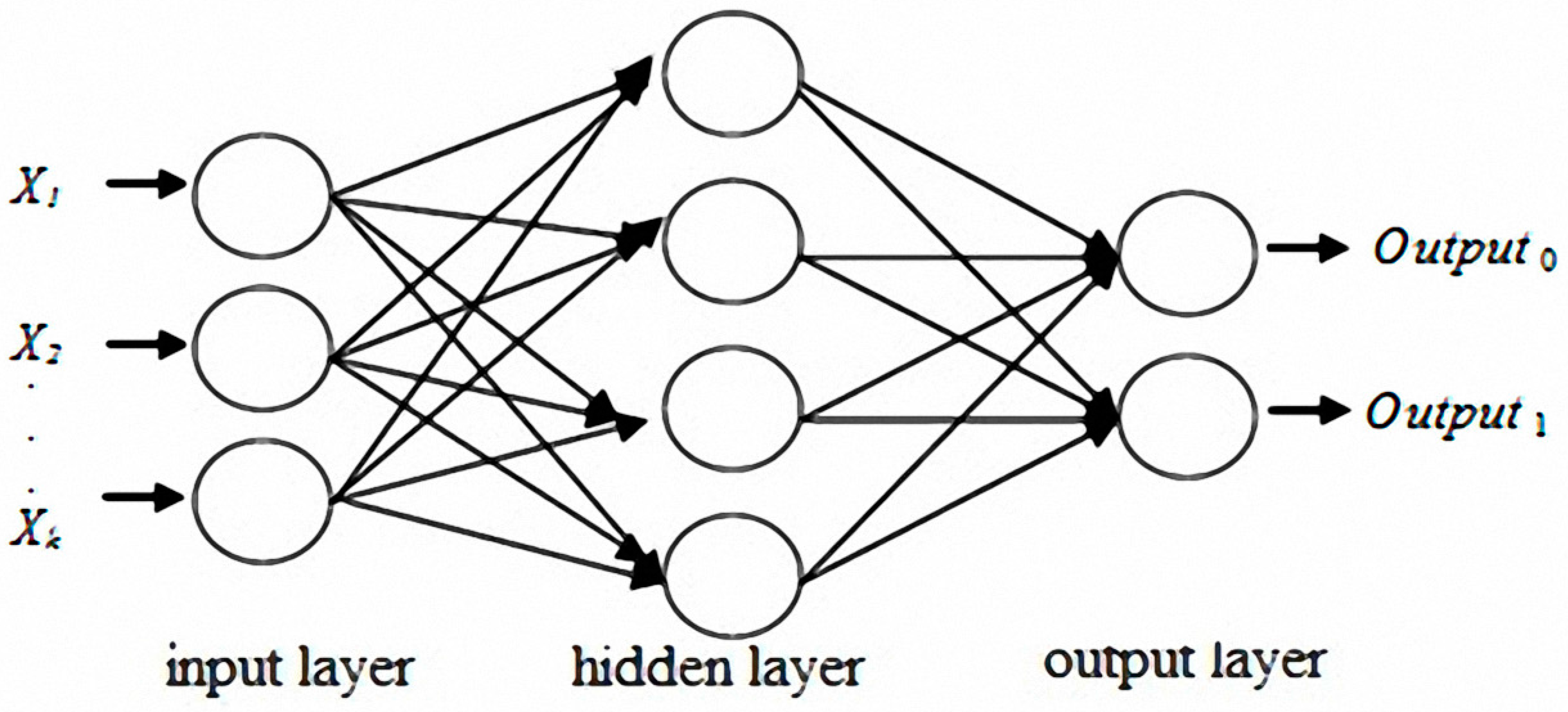
The original concept of neural networks was derived from biological nervous systems. Biological thinking is emulated using computers. Learning and thinking by using data generate answers for specific problems. A number of models have been presented for the development of neural networks. The most influential of these models is multilayer perceptron (MLP) [38,39,40,41]. MLP typically includes a number of layers, which are classified as input, hidden, or output layers. Each neuron in the input layer corresponds to a predictor variable, and the number of neurons is equal to the number of predictor variables. The number of neurons in the output layer is identical to the number of response variables [42,43]. Figure 3 shows that one or multiple hidden layers are possible.
The discussed studies revealed that the MTS, logistic regression and neural networks all demonstrated excellent discrimination when solving binary classification problems with multivariate data. The characteristic variable selections and classification prediction results obtained using the MTS are comparatively robust under identical data conditions. Therefore, the MTS architecture was analyzed, and logistic regression models and neural networks were used to improve the tablet PC product testing process. The differences among these three methods were subsequently compared and discussed.
3. Analysis Results and Discussion
3.1. MTS Analysis
The 56 test item variables were assigned codes X1–X56. Next, 450 pieces of data (i.e., 450 tablet PCs) were randomly selected from the production line, of which 300 were used as the training group. Within this group, 268 were normal and 32 were abnormal data samples. The other 150 pieces of data were used as the validation group to validate the model. Table 1 details the collected sample data (see the Appendix A).
The 268 normal samples from the training group data were used as a basis for constructing the Mahalanobis space, which contained the mean, standard deviation, and correlation coefficient inverse matrix of the data group. After the Mahalanobis space (or base space) was constructed, the Mahalanobis distances of the normal and abnormal samples in the training and validation groups were calculated and plotted on graphs. Figure 4 and Figure 5 illustrate the Mahalanobis distance distributions of the training and validation groups, respectively. When the threshold was 2.0, the accuracy of the training group and validation group was 99.3% (Table 2). Therefore, the measurement scale of the model constructed using the 56 variables was reliable and effective at this stage. Next, the possibility of achieving acceptable production testing accuracy after reducing the number of variables and using fewer test items was investigated.
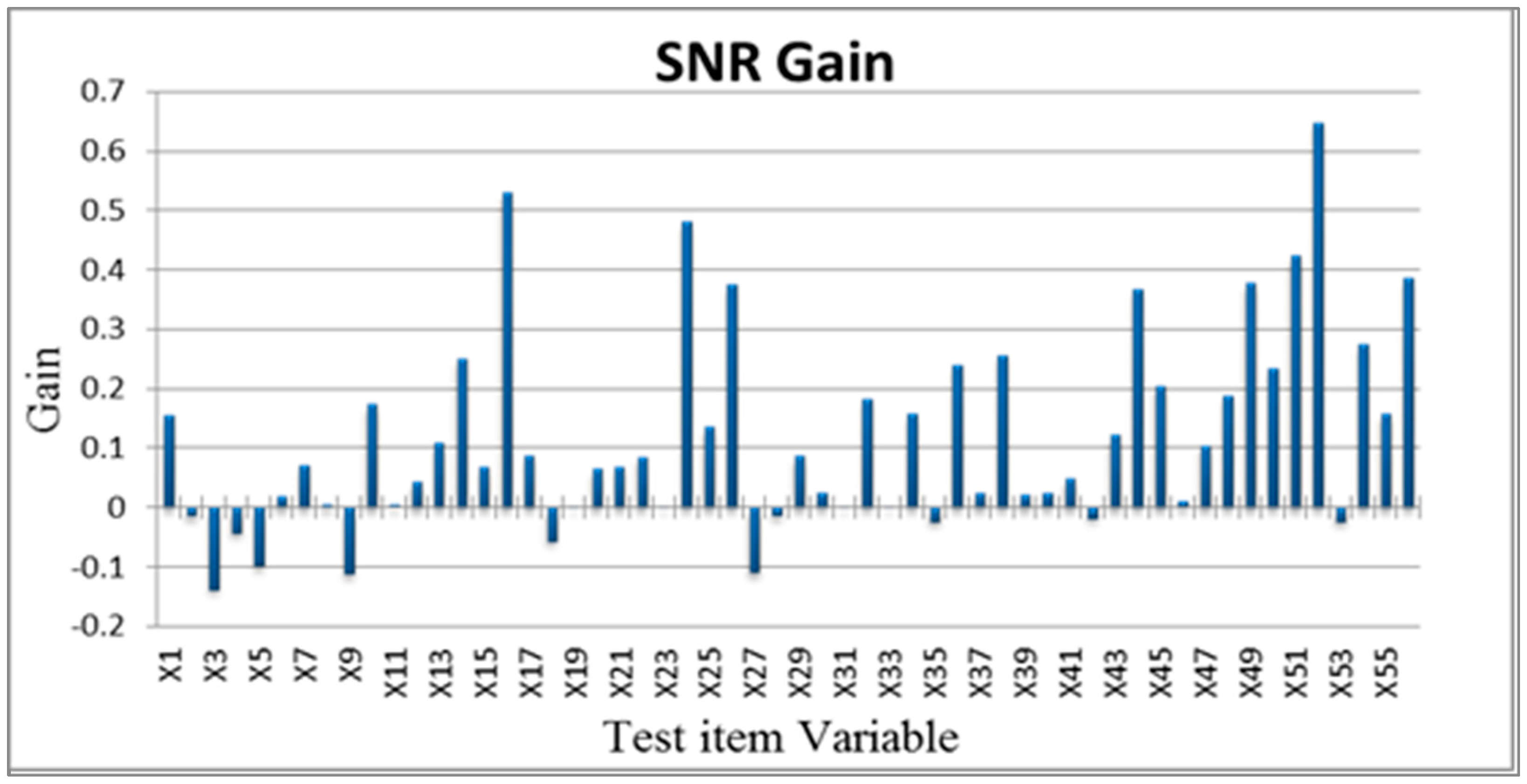
The most critical variables affecting tablet PC production testing were identified, and unnecessary variables were removed. Orthogonal arrays were used to investigate which test items affected the tablet PC production testing results. First, each variable was assigned to Level 1 (for used variables) or Level 2 (for unused variables). Next, these variables were distributed to the appropriate orthogonal arrays. In this study, 56 variables were used. Therefore, L64(263) orthogonal arrays were employed. The 32 abnormal samples in the training group were used to calculate 32 corresponding Mahalanobis distances. The larger-the-better SN ratio was also used, based on the principle that a high SN ratio and a high increment in variable effect were favorable. Figure 6 illustrates the effect increments for each variable.
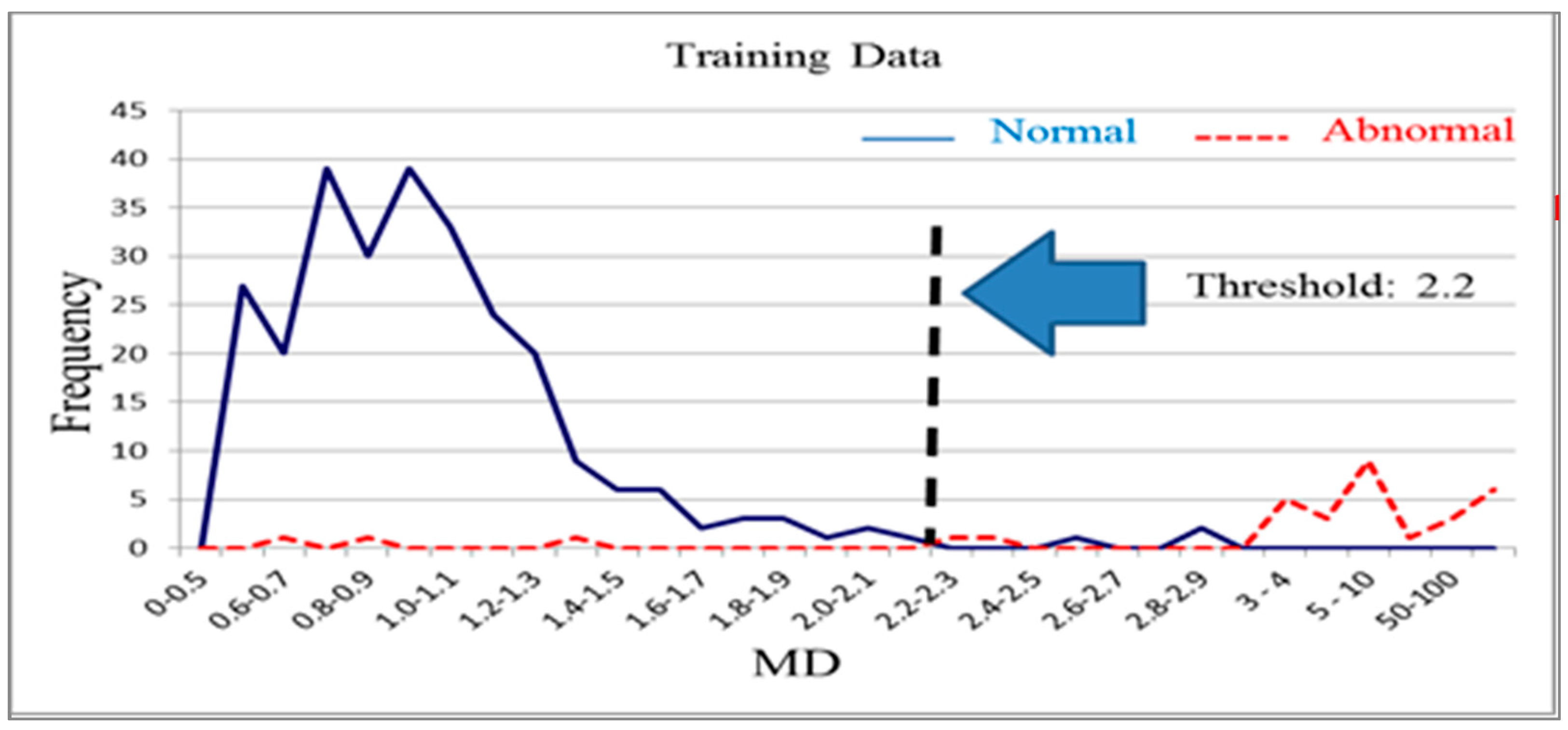
The variables were screened on the basis of their effect increments (>0, >0.1, >0.2, >0.3 and >0.4), which reduced the 56 original test items to 45, 24, 14, 8 and 4, respectively. Reduced models were then established after the corresponding variables were removed. When the effect increment was greater than 0.2, the training group and validation group accuracy was 98%. The final characteristic variables selected were X14, X16, X24, X26, X36, X38, X44, X45, X49, X50, X51, X52, X54 and X56, a total of 14 characteristic variables. The normal sample data from the training group and 14 critical test item variables were used after screening to reconstruct the Mahalanobis space. An abnormal sample was used to confirm the measurements of the reduced model. Figure 7 and Figure 8 present the frequency distributions derived from these data.
Type-I and type-II error minimization were used as a basis for determining the threshold of 2.2, which resulted in an accuracy of 98%. Next, the sample data from the validation group were used to confirm that the accuracy was also 98% when the variables were reduced to 14 items and the threshold was set to 2.2 (Table 3). Therefore, the number of test items used in the tablet PC product testing process was reduced from the original 56 items to 14 items by using the MTS analysis method. Validation results for the different groups still indicated high accuracy after this reduction. The MTS is thus a feasible method for screening test item variables.
3.2. Logistic Regression Analysis
The logistic regression analysis data were identical to those used in the MTS analysis in the previous section. The 450 pieces of data were divided into 300 pieces of training data and 150 pieces of validation data. Next, logistic regression analysis was used to construct a model. A binary variable (0 = normal sample, 1 = abnormal sample) was the dependent variable and the 56 test variables were the independent variables.
The results of the coefficient test of the binary logistic regression analysis variables from SPSS software were used to determine the number of variables that were insignificant. This would indicate only the characteristic variables that had a substantial effect on tablet PC product testing abnormalities. These crucial key factors were then reconsidered to establish a logistic regression model.
Forward stepwise regression was used to screen the 56 original characteristic variables, yielding 15 crucial factors. These 15 characteristic variables were used to construct an optimal model configuration by using logistic regression. A register value of 0.05 and a removal value of 0.1 were adopted as testing standards for determining the stepwise variable probability. The reduced equation based on the stepwise regression analysis results is expressed as follows:
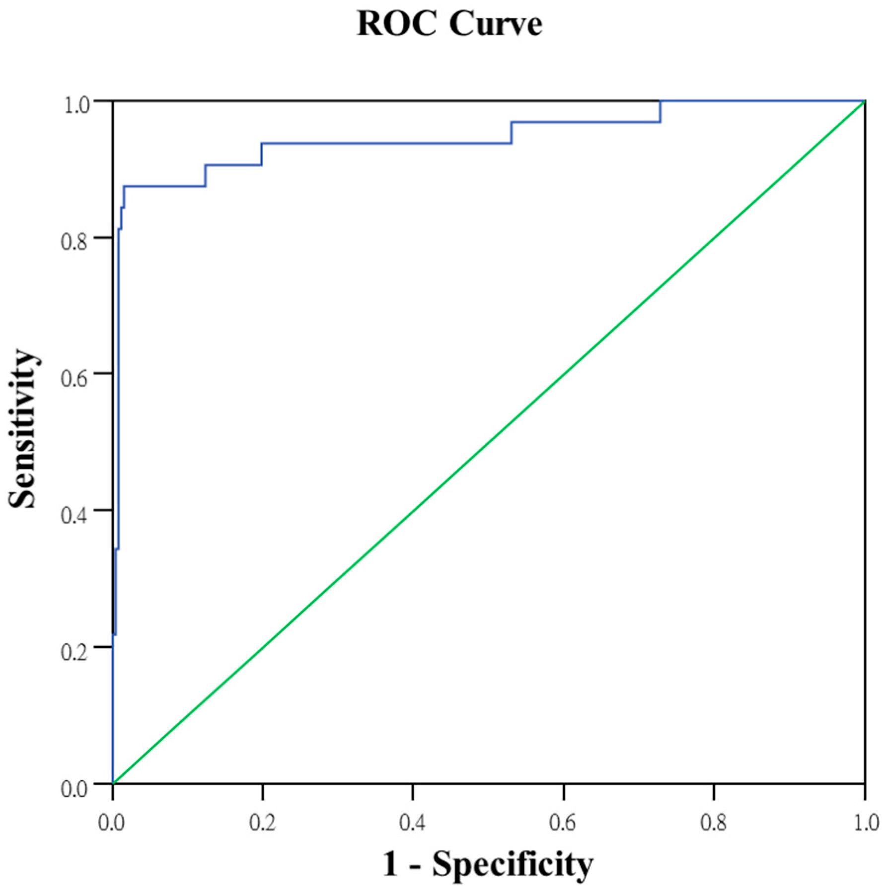
The selected variables were X1, X13, X18, X20, X24, X25, X38, X41, X43, X45, X47, X48, X49, X51 and X55. The area under the logistic regression receiver operating characteristic (ROC) curve (Figure 9) was 0.946.
The 300 pieces of training data (268 normal samples and 32 abnormal samples) were entered into the reduced equation. Type-I and type-II error minimization were used as a basis for determining the threshold. The accuracy was 97.3% when the separated value was set to 0.4. The results presented in Table 4 revealed that the testing accuracy for the validation group was 93.3% when the separated value was 0.4. Therefore, conventional logistic regression is a feasible method for test item variable screening.
3.3. Neural Network Analysis
A neural network was used to construct a prediction model for determining accuracy in tablet PC product testing. A random sample of 450 pieces of data was divided into training (300 pieces of data) and retention (validation) groups (150 pieces of data). MLP program for neural networks included in SPSS was used to generate the prediction model. The input layer nodes were the 56 characteristic variables used for testing. The model had one hidden layer, with the hyperbolic tangent function as the start function. The output layer contained two nodes: normal product and abnormal product.
The accuracy of the testing of the 300 pieces of data (268 normal and 32 abnormal samples) in the training group, calculated using the neural network, was 99.7%, which indicated excellent training. Table 5 lists the importance of each of the test variables. An importance value greater than 0.21 and a normalized importance greater than 30% were used as the screening criteria. Sixteen critical characteristic variables were obtained for constructing the reduced neural network model.
The possibility of achieving satisfactory production testing accuracy after using neural network analysis to reduce the number of test items was subsequently investigated. After performing calculations using the neural network, the testing accuracy of the 300 pieces of training data and 150 pieces of retention (validation) data was 99.3% and 94.7%, respectively (Table 6). The area under the neural network ROC curve was 1.0 (Figure 10). Therefore, the neural network is also effective for predicting tablet PC product yield.
3.4. Comparison of Results and Efficiency Improvement
Table 7 presents a comparison of accuracy based on the MTS, logistic regression, and neural network analysis results. The accuracy was 98% for both the training and validation groups in the reduced model of the tablet PC product testing process constructed using the MTS. In the reduced model comprising crucial variables identified using logistic regression, testing of the training and validation groups demonstrated accuracies of 97.3% and 93.3%, respectively. When the neural network analysis was performed, testing of the training and validation groups exhibited accuracies of 99.3% and 94.7%, respectively. These results indicated that all three methods produced strong class prediction accuracy and the MTS was not inferior to conventional logistic regression analysis or neural network analysis. The MTS produced a higher accuracy when determining product yield using a reduced model established using the training group data than the other two methods. Nevertheless, the MTS method features high stability and an accuracy rate higher than 98%. Thus, the MTS, which involves using data mining and classification methods to reduce attribute variables for building prediction models, demonstrates high discrimination ability in practice [16].
The type-I errors (i.e., the analysis methods showed that tablet PCs were abnormal products when in fact they were normal products), and type-II errors (i.e., the tablets PCs were abnormal products that failing to judge as normal products) were identified for each method. Generally, the cost of type-I errors is incurred through the need for product retesting. However, the cost of type-II errors is more severe and includes costs incurred through return material authorizations, customer complaints, or recalls. Therefore, reduced models for product testing are used to avoid type-II errors. The MTS analysis method resulted in the fewest type-II errors, whereas the logistic regression analysis demonstrated the least favorable performance (Table 8).
The three analysis methods were used to screen the characteristic variables. The MTS reduced the 56 original test items to 14, logistic regression reduced them to 15, and neural networks reduced them to 16. Table 9 reveals that X24, X38, X45, X49 and X51 were selected by all three analysis methods.
In summary, the product testing accuracy of the MTS after the elimination of insignificant test items was superior to that of conventional logistic regression analysis and neural network analysis. The reduction in variables saved time during the product testing process, which indicates the method’s cost effectiveness. Additionally, the reduction in the number of test items enabled the five testing stations used in the original manufacturing process to be reduced to three. The time typically required for the manufacturing process was reduced from 2460 to 1200 s, and the original 10 testers was reduced to 5. Overall, production efficiency approximately doubled. The required number of test machines was also reduced. In addition to saving on machine installation costs, the use of this method also reduced machine maintenance and related personnel costs.
4. Conclusions
The MTS is a suitable method for solving classification problems because it detects the severity of abnormal samples and uses orthogonal arrays and SN ratios to verify whether the selected variables are appropriate. The crucial screened characteristic variables can be used to construct reduced class prediction models with high total accuracy while maintaining the model’s ability to identify each class [44,45]. Therefore, the MTS is appropriate for class prediction applications in various fields. In addition, the robustness of the MTS regarding characteristic variable selection and class prediction will enable engineering staff to understand product characteristics and evaluate the suitability of tablet PC product test items. Through the removal of test items that offer little contribution, accurate and rapid product detection can be achieved. This reduces the number of testing stations and testers, thereby decreasing testing costs and enhancing industrial competitiveness.
MTS theory was employed to analyze tablet PC product test items for Technology Company A. The Mahalanobis distance critical values were used to differentiate between defective and nondefective products. Orthogonal arrays and SN ratios were used to screen crucial test items. Finally, validation group sample data were used to determine the accuracy of the reduced model. These results were compared with those obtaining using logistic regression and neural network analysis methods. The results indicated that the predictive power of the MTS after reducing the number of test items was 98%, superior to that of conventional logistic regression and neural networks, which had predictive powers of 93.3% and 94.7%, respectively. After reduction, the MTS model contained 14 test items, which was fewer than the number in the logistic regression (15 items) and neural network (16 items) models. Optimization of the testing process using the MTS analysis method provided suitable test items and a reduced model for product testing. This facilitated formulating a more efficient test station configuration and also effectively reduced investment costs for testers and equipment. In addition to improvements in production efficiency on the production line and acceleration of a company’s possible reaction to market demand, reductions in equipment and related expenses ensure the competitiveness of a company in the overall market.
Acknowledgments
This work was supported by Provincial Nature Science Foundation of Guangdong (Nos. 2015A030310271 and 2015A030313679); The National Social Science Foundation of China (No. 15BGL019); Shanghai Social Science Foundation (No. 2014BGL004); and Zhongshan City Science and Technology Bureau Project.
Author Contributions
Writing: Chi-Feng Peng, Li-Hsing Ho, and Sang-Bing Tsai. Providing case and idea: Chi-Feng Peng and Yin-Cheng Hsiao. Providing revision advice: Yuming Zhai, Quan Chen, Li-Chung Chang, and Zhiwen Shang.
Conflicts of Interest
The authors declare no conflict of interest.
Appendix A

Table A1.
Test items of Tablet PC.
| Variable | Test Item | Note | Variable | Test Item | Note |
|---|---|---|---|---|---|
| X1 | Piezo | PT1-Buzzer | X29 | GSM PhaseErrRMS | PT3-GSM |
| X2 | USB Port | PT1-USB | X30 | GSM BER | PT3-GSM |
| X3 | SD Card | PT1-SDCard | X31 | GSM BLER | PT3-GSM |
| X4 | Battery Voltage(AD) | PT2-Adapter | X32 | EDGE TxPower | PT3-EDGE |
| X5 | B-to-B Amp(AD) | PT2-Adapter | X33 | EDGE FreqErr | PT3-EDGE |
| X6 | Charge Voltage(AD) | PT2-Adapter | X34 | EDGE PhaseErrPeak | PT3-EDGE |
| X7 | Charge Amp(AD) | PT2-Adapter | X35 | EDGE PhaseErrRMS | PT3-EDGE |
| X8 | App Voltage(AD) | PT2-Adapter | X36 | EDGE BER | PT3-EDGE |
| X9 | Battery Voltage | PT2-Battery | X37 | EDGE BLER | PT3-EDGE |
| X10 | B-to-B Amp | PT2-Battery | X38 | WCDMA TxPower | PT3-WCDMA |
| X11 | Charger Voltage | PT2-Battery | X39 | WCDMA FreqErr | PT3-WCDMA |
| X12 | Charger Amp | PT2-Battery | X40 | WCDMA PhaseErrPeak | PT3-WCDMA |
| X13 | App Voltage | PT2-Battery | X41 | WCDMA PhaseErrRMS | PT3-WCDMA |
| X14 | Wi-Fi RSSI | PT2-WLAN | X42 | WCDMA BER | PT3-WCDMA |
| X15 | Wi-Fi Throughput | PT2-WLAN | X43 | WCDMA BLER | PT3-WCDMA |
| X16 | Audio Freq. | PT2-Speaker | X44 | TP Calibrate | PT4-LCD |
| X17 | Output Level | PT2-Speaker | X45 | Bright | PT4-LCD |
| X18 | Mute | PT2-Speaker | X46 | Contrast | PT4-LCD |
| X19 | Stereo Phasing | PT2-Speaker | X47 | Point Defected | PT4-LCD |
| X20 | Dynamic Range | PT2-Speaker | X48 | LAN Port | PT4-LAN |
| X21 | Output Level | PT2-EarJack | X49 | Zigbee TxPower | FT-Zigbee |
| X22 | Mute | PT2-EarJack | X50 | Wi-Fi RSSI | FT-WLAN |
| X23 | Stereo Phasing | PT2-EarJack | X51 | Wi-Fi Throughput | FT-WLAN |
| X24 | Dynamic Range | PT2-EarJack | X52 | Touch Panel | FT-LCD |
| X25 | Amplitude | PT2-EarJack | X53 | Voice Test | FT-Voice |
| X26 | GSM TXPower | PT3-GSM | X54 | USB Port | FT-USB |
| X27 | GSM FreqErr | PT3-GSM | X55 | SD Card | FT-SDCard |
| X28 | GSM PhaseErrPeak | PT3-GSM | X56 | Piezo | FT-Buzzer |
References
- Gartner Says Worldwide Traditional PC, Tablet, Ultramobile and Mobile Phone Shipments to Grow 4.2 Percent in 2014. Available online: http://www.gartner.com/newsroom/id/2791017 (accessed on 22 August 2017).
- NPD DisplaySearch Announced It Forecasts that Global Tablet Shipments Will Overtake Notebook Shipments in 2016. Available online: http://www.hughsnews.ca/tablets-to-overtake-notebook-pcs-0035757 (accessed on 22 August 2017).
- Wang, J.; Teng, A. ODMs and EMS Companies Are Ready to Capture Their Share of the Future Wearable Device Market; Gartner, Inc.: Stamford, CT, USA, 2013. [Google Scholar]
- Choi, J.Y.; Shin, J.W.; Lee, J.S. Strategic demand forecasts for the tablet PC market using the Bayesian mixed logit model and market share simulations. Behav. Inform. Technol. 2013, 32, 1177–1190. [Google Scholar] [CrossRef]
- Taguchi, G.; Jugulum, R. The Mahalanobis-Taguchi Strategy: A Pattern Technology System; John Wiley & Sons, Inc.: Hoboken, NJ, USA, 2002. [Google Scholar]
- Lin, H.L. The use of the Taguchi method with grey relational analysis and a neural network to optimize a novel GMA welding process. J. Intell. Manuf. 2012, 23, 1671–1680. [Google Scholar] [CrossRef]
- Wang, Z.; Wang, Z.; Tao, L.; Ma, J. Fault diagnosis for bearing based on Mahalanobis-Taguchi system. In Proceedings of the 2012 IEEE Conference on Prognostics and System Health Management (PHM), Beijing, China, 23–25 May 2012. [Google Scholar]
- Soylemezoglu, A.; Sarangapani, J.; Saygin, C. Mahalanobis Taguchi system (MTS) as a prognostics tool for rolling element bearing failures. J. Manuf. Sci. Eng. 2010, 132. [Google Scholar] [CrossRef]
- Lee, Y.C.; Teng, H.L. Predicting the financial crisis by Mahalanobis-Taguchi system-examples of Taiwan’s electronic sector. Expert Syst. Appl. 2009, 36, 7469–7478. [Google Scholar] [CrossRef]
- Jobi-Taiwo, A.A. Data Classification and Forecasting Using the Mahalanobis-Taguchi Method. Master’s Thesis, Missouri University of Science and Technology, Rolla, MO, USA, 2014. [Google Scholar]
- Taguchi, G.; Chowdhury, S.; Wu, Y. The Mahalanobis-Taguchi System; McGraw-Hill: New York, NY, USA, 2001. [Google Scholar]
- Soylemezoglu, A.; Jagannathan, S.; Saygin, C. Mahalanobis-Taguchi system as a multi-sensor based decision making prognostics tool for centrifugal pump failures. IEEE Trans. Reliab. 2011, 60, 864–878. [Google Scholar] [CrossRef]
- Wang, N.; Saygin, C.; Sun, S. Impact of Mahalanobis space construction on effectiveness of Mahalanobis-Taguchi system. Int. J. Ind. Syst. Eng. 2013, 13, 233–249. [Google Scholar] [CrossRef]
- Su, C.T. Quality Engineering; Chinese Society for Quality: Taipei, Taiwan, 2002. [Google Scholar]
- Su, C.T.; Chou, C.J.; Hung, S.H.; Wang, P.C. Adopting the healthcare failure mode and effect analysis to improve the blood transfusion processes. Int. J. Ind. Eng. 2012, 19, 320–329. [Google Scholar]
- Lee, Y.C.; Hsiao, Y.C.; Peng, C.F.; Tsai, S.B.; Wu, C.H.; Chen, Q. Using Mahalanobis–Taguchi system, logistic regression, and neural network method to evaluate purchasing audit quality. J. Eng. Manuf. 2015, 229, 3–12. [Google Scholar] [CrossRef]
- Buenviaje, B.; Bischoff, J.E.; Roncace, R.A.; Willy, C.J. Mahalanobis-Taguchi system to identify preindicators of delirium in the ICU. IEEE J. Biomed. Health Inform. 2016, 20, 1205–1212. [Google Scholar] [CrossRef] [PubMed]
- Saygin, C.; Mohan, D.; Sarangapani, J. Real-time detection of grip length during fastening of bolted joints: A Mahalanobis-Taguchi system (MTS) based approach. J. Intell. Manuf. 2010, 21, 377–392. [Google Scholar] [CrossRef]
- Su, C.T.; Hsiao, Y.H. Multiclass MTS for simultaneous feature selection and classification. IEEE Trans. Knowl. Data Eng. 2009, 21, 192–205. [Google Scholar]
- Taguchi, G.; Jugulum, R. New trends in multivariate diagnosis. Indian J. Stat. 2000, 62, 233–248. [Google Scholar]
- Hsiao, Y.H.; Su, C.T. Multiclass MTS for saxophone timbre quality inspection using waveform-shape-based features. IEEE Trans. Syst. Man Cybern. B Cybern. 2009, 39, 690–704. [Google Scholar] [CrossRef] [PubMed]
- Su, C.T.; Chen, K.H.; Chen, L.F.; Wang, P.C.; Hsiao, Y.H. Prediagnosis of obstructive sleep apnea via multiclass MTS. Comput. Math. Methods Med. 2012, 2012. [Google Scholar] [CrossRef] [PubMed]
- Taketoshi, R.; Akihito, S.J.; Kenji, O.T. The yieldenhancement methodology for invisible defects using the MTS method. Trans. Semicond. Manuf. 2005, 18, 561–568. [Google Scholar]
- Jobi-Taiwo, A.A.; Cudney, E.A. Mahalanobis-Taguchi system for multiclass classification of steel plates fault. Int. J. Qual. Eng. Technol. 2015, 5, 25–39. [Google Scholar] [CrossRef]
- Tsai, S.B.; Huang, C.Y.; Wang, C.K.; Chen, Q.; Pan, J.; Wang, G.; Wang, J.; Chin, T.C.; Chang, L.C. Using a mixed model to evaluate job satisfaction in high-tech industries. PLoS ONE 2016, 11, e0154071. [Google Scholar] [CrossRef] [PubMed]
- Cudney, E.A.; Paryani, K.; Ragsdell, K.M. Applying the Mahalanobis-Taguchi system to vehicle handling. Concurr. Eng. 2006, 14, 343–354. [Google Scholar] [CrossRef]
- Kim, S.B.; Tsui, K.; Sukchotrat, T.; Chen, V.C.P. A comparison study and discussion of the Mahalanobis-Taguchi System. Ind. Syst. Eng. 2009, 4, 631–644. [Google Scholar] [CrossRef]
- Taguchi, G.; Chowdhury, S.; Wu, Y. Taguchi’s Quality Engineering Handbook; Wiley: New York, NY, USA, 2005. [Google Scholar]
- Ghasemi, E.; Aaghaie, A.; Cudney, E.A. Mahalanobis Taguchi system: A review. Int. J. Qual. Reliab. Manag. 2015, 32, 291–307. [Google Scholar] [CrossRef]
- Pan, J.N.; Pan, J.B.; Lee, C.Y. Finding and optimising the key factors for the multiple-response manufacturing process. Int. J. Prod. Res. 2009, 47, 2327–2344. [Google Scholar] [CrossRef]
- Berkson, J. Application of the logistic function to bio-assay. J. Am. Stat. Assoc. 1944, 9, 357–365. [Google Scholar]
- Reichert, A.; Cho, C.C.; Wagner, G.M. An examination of the conceptual issues involved in developing credit-scoring models. J. Bus. Econ. Stat. 1983, 1, 101–114. [Google Scholar]
- Lee, H.; Jo, H.; Han, I. Bankruptcy prediction using case based reasoning, neural networks, and discriminant analysis. Expert Syst. Appl. 1997, 13, 97–108. [Google Scholar]
- Kong, X.Z. Reducing Test Items of TFT-LCD Product by Using Neural Networks. Master’s Thesis, National Chiao Tung University, Hsinchu, Taiwan, 2007. [Google Scholar]
- Chen, L.F.; Su, C.T.; Chen, M.H. A neural-network approach for defect recognition in TFT-LCD photolithography process. IEEE Trans. Electron. Packag. Manuf. 2009, 32, 1–8. [Google Scholar] [CrossRef]
- Hsieh, W.K. The Application of Neuron Network to the Forecasting of a Make to Stock Paper Production System. Master’s Thesis, National Taiwan University of Technology, Taipei, Taiwan, 2007. [Google Scholar]
- Wang, W.Z.; Lin, W.C.; Lai, Z.H.; Chen, H.M. Data mining applied to the predictive model of triage system in emergency department—A case of a medical center in Taiwan. J. Qual. 2008, 15, 283–291. [Google Scholar]
- Zhang, G.; Hu, M.Y.; Patuwo, B.E.; Indro, D.C. Artificial neural networks in bankruptcy prediction: General framework and cross-validation analysis. Eur. J. Oper. Res. 1999, 116, 16–32. [Google Scholar] [CrossRef]
- Cudney, E.; Hong, J.; Jugulum, R.; Paryani, K.; Ragsdell, K.; Taguchi, G. An evaluation of Mahalanobis-Taguchi system and neural network for multivariate pattern recognition. J. Ind. Syst. Eng. 2007, 1, 139–150. [Google Scholar]
- Kuo, C.F.; Hsu, C.T.; Fang, C.H.; Chao, S.M.; Lin, Y.D. Automatic defect inspection system of colour filters using Taguchi-based neural network. Int. J. Prod. Res. 2013, 51, 1464–1476. [Google Scholar] [CrossRef]
- Li, D.C.; Chang, C.C.; Liu, C.W.; Chen, W.C. A new approach for manufacturing forecast problems with insufficient data: The case of TFT–LCDs. J. Intell. Manuf. 2013, 24, 225–233. [Google Scholar] [CrossRef]
- Teng, C.J.; Yang, Y.K.; Hsieh, M.H.; Jeng, M.C. Optimization of wire electrical discharge machining of pure tungsten using neural network and response surface methodology. J. Eng. Manuf. 2011, 225, 841–852. [Google Scholar]
- Tsai, S.B.; Chien, M.F.; Xue, Y.; Li, L.; Jiang, X.; Chen, Q.; Zhou, J.; Wang, L. Using the fuzzy DEMATEL to determine environmental performance: A case of printed circuit board industry in Taiwan. PLoS ONE 2015, 10, e0129153. [Google Scholar] [CrossRef] [PubMed]
- Su, C.T.; Hsiao, Y.H. An evaluation of the robustness of MTS for imbalanced data. IEEE Trans. Knowl. Data Eng. 2007, 19, 1321–1332. [Google Scholar] [CrossRef]
- Ren, J.T.; Xing, X.C.; Cai, Y.W.; Chen, J. A method of multi-class faults classification based-on Mahalanobis-Taguchi system using vibration signals. In Proceedings of the 2011 9th International Conference on Reliability, Maintainability and Safety (ICRMS), Guiyang, China, 12–15 June 2011. [Google Scholar]
Figure 1.
Global tablet PC shipment forecasts (unit: thousand). Source: NPD DisplaySearch Quarterly Mobile PC Shipment and Forecast Report.
Figure 1.
Global tablet PC shipment forecasts (unit: thousand). Source: NPD DisplaySearch Quarterly Mobile PC Shipment and Forecast Report.
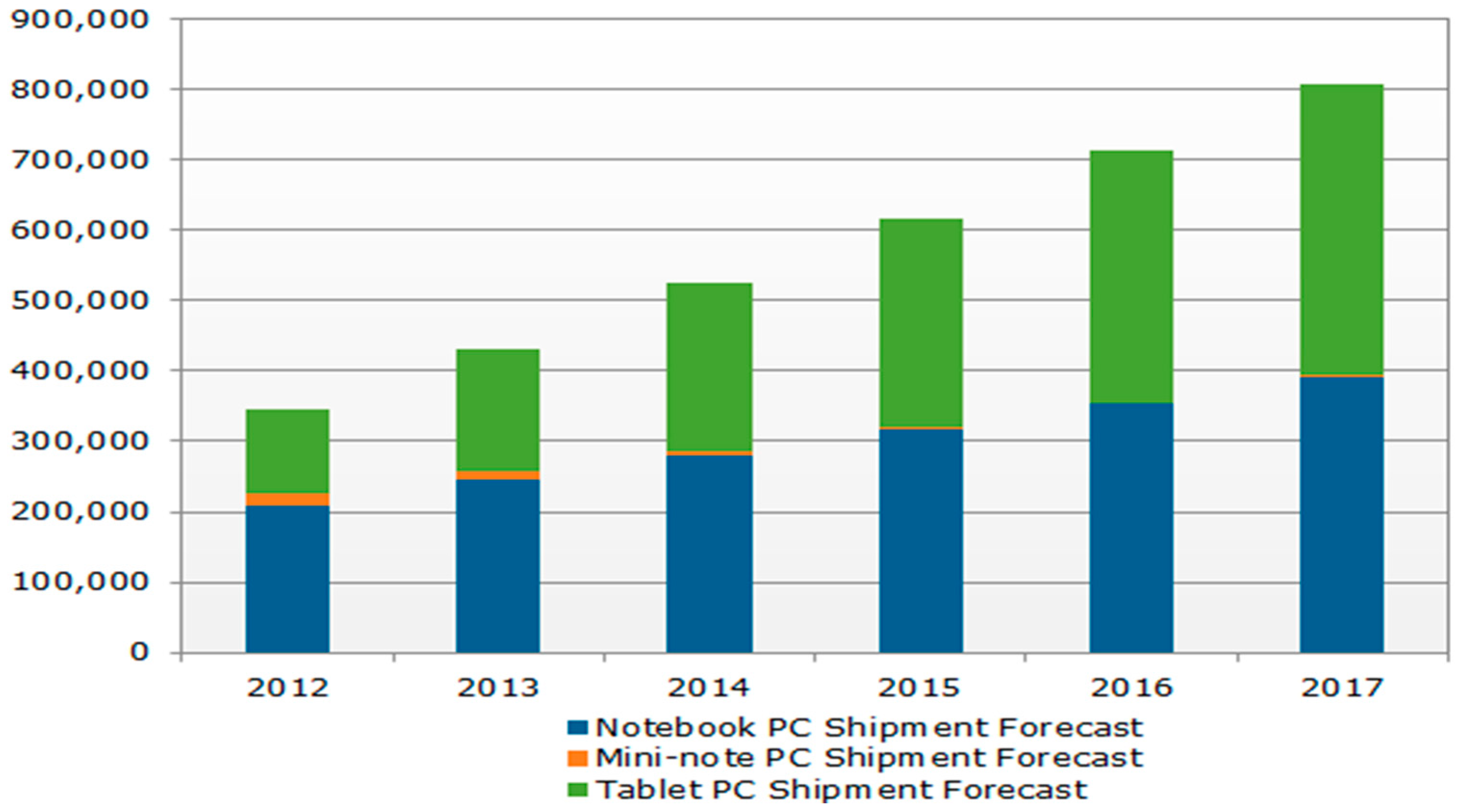
Figure 2.
Tablet PC production testing process.
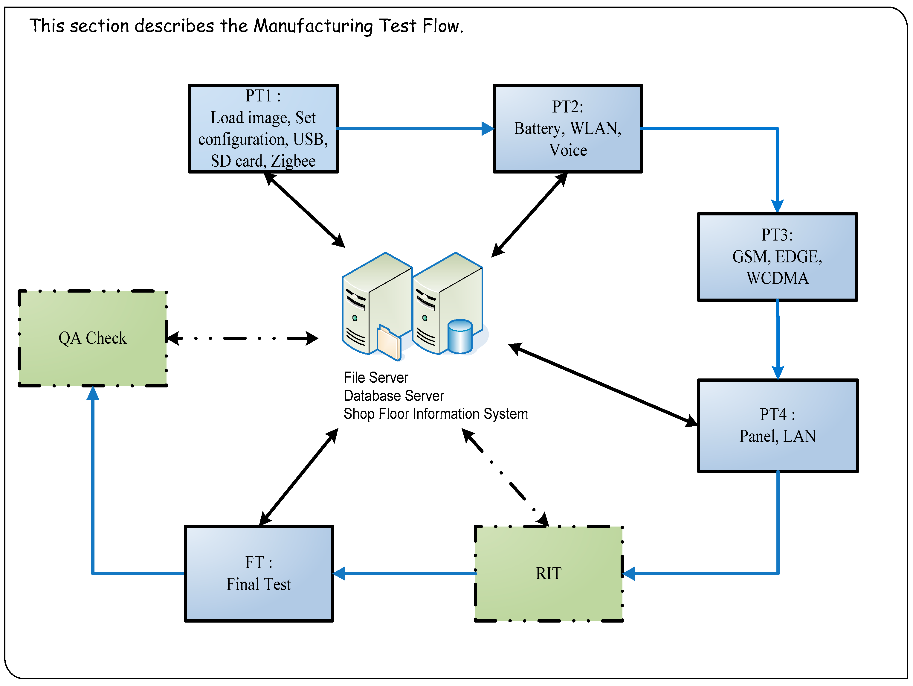
Figure 3.
Neural network example.

Figure 4.
Mahalanobis distance distribution for the training group (k = 56).
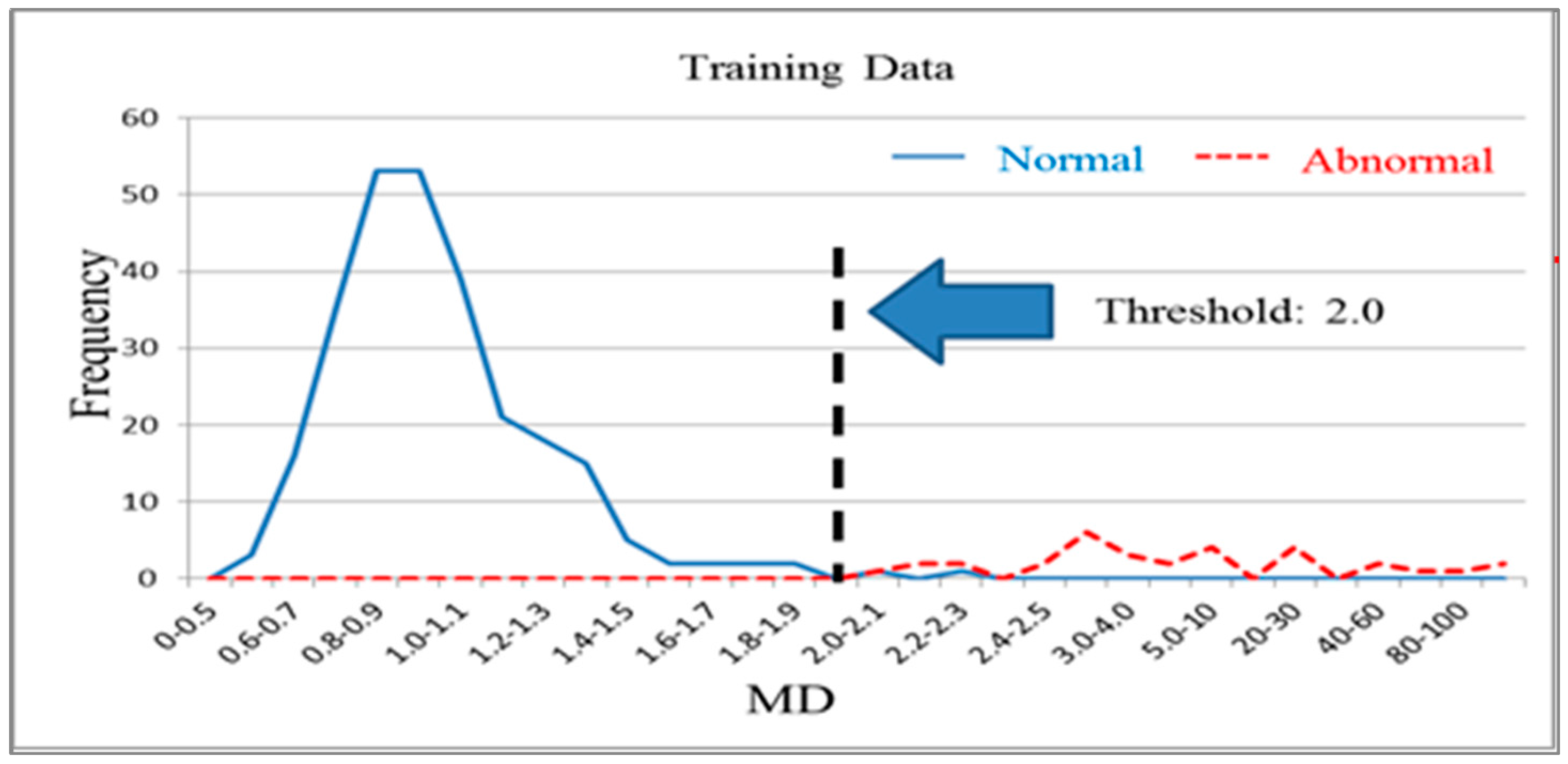
Figure 5.
Mahalanobis distance distribution for the validation group (k = 56).
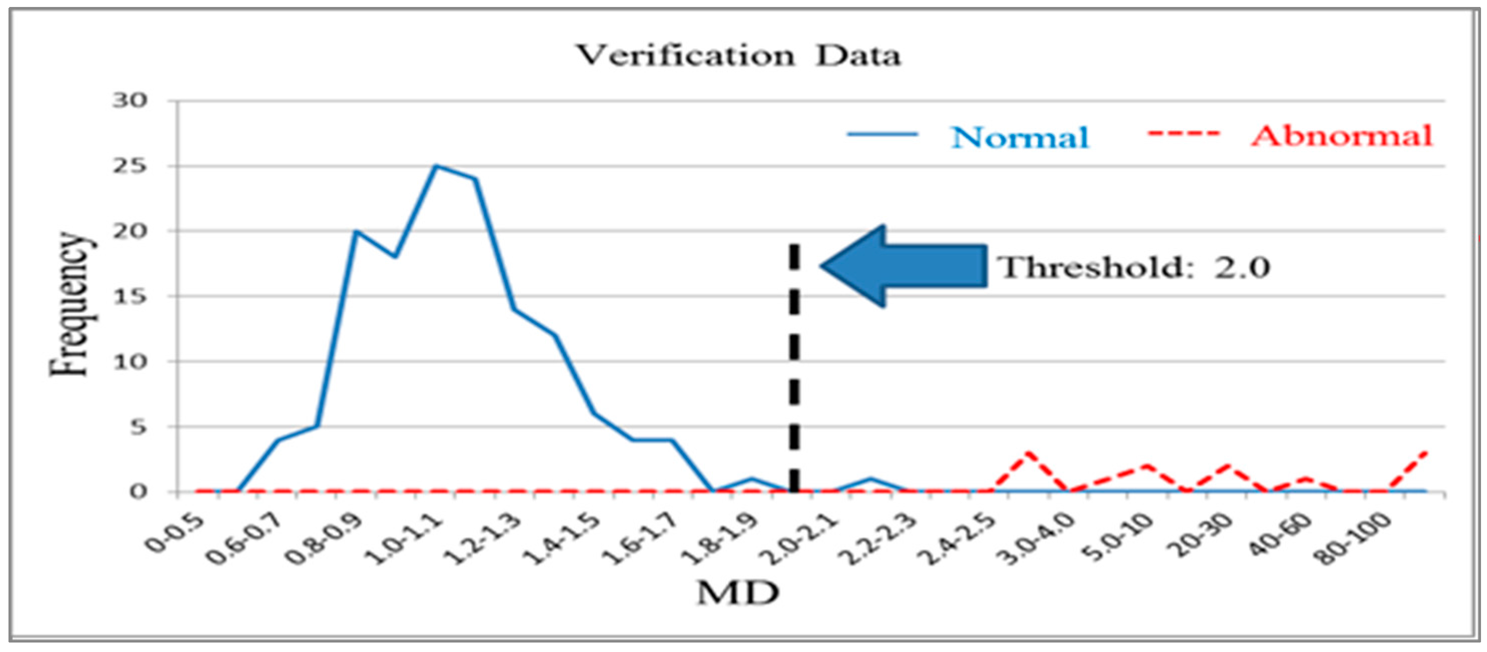
Figure 6.
Variable effect increments.

Figure 7.
Mahalanobis distance distribution for the training group (k = 14).

Figure 8.
Mahalanobis distance distribution for the validation group (k = 14).
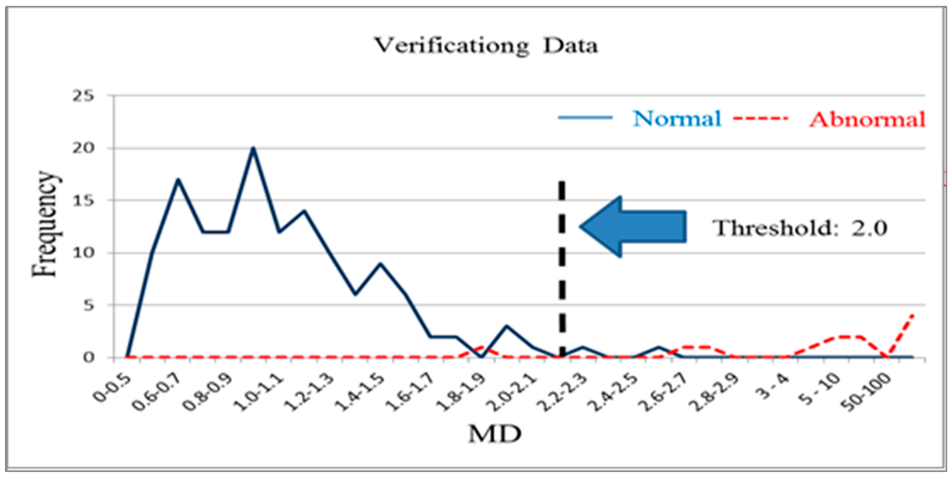
Figure 9.
Logistic regression ROC curve.

Figure 10.
Neural network ROC curve.
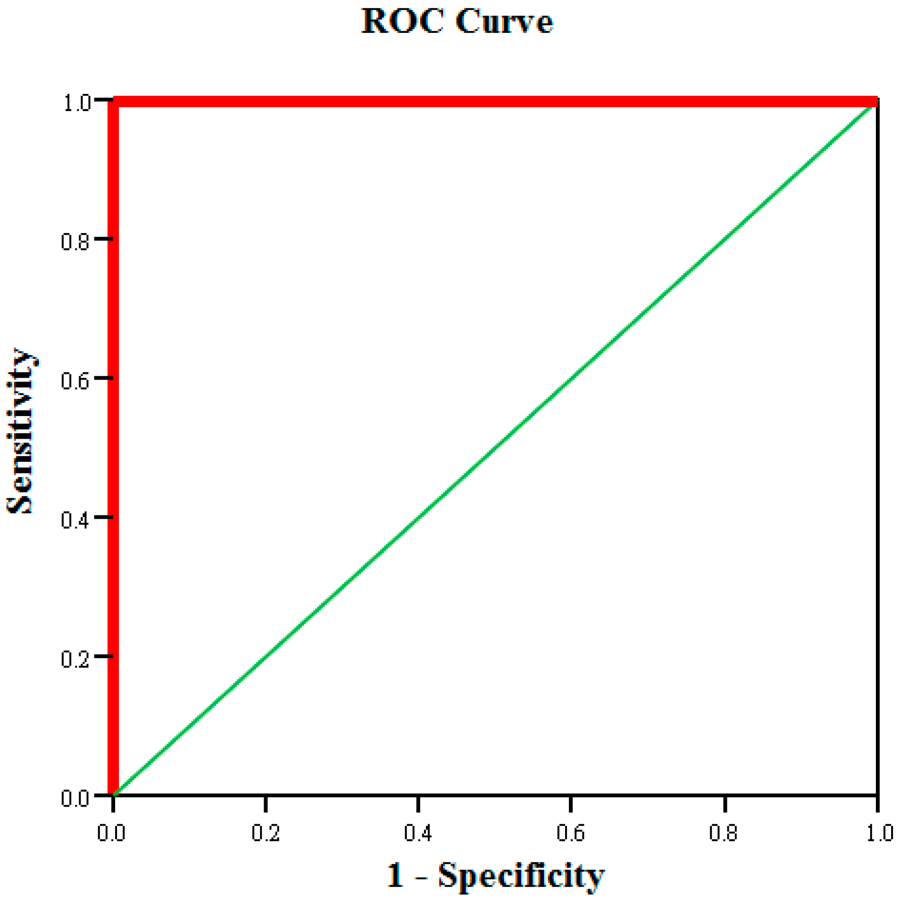
Table 1.
Sample data.
| Normal Samples | Abnormal Samples | Total | |
|---|---|---|---|
| Training Group | 268 | 32 | 300 |
| Validation Group | 138 | 12 | 150 |
Table 2.
Accuracy of the results for the training and validation groups using MTS analysis (Full Model).
Table 2.
Accuracy of the results for the training and validation groups using MTS analysis (Full Model).
| Training Group | Normal (R) | Abnormal (R) | Accuracy | |
| Normal | 266 | 2 | 99.3% | |
| Abnormal | 0 | 32 | ||
| Validation Group | Normal (R) | Abnormal (R) | Accuracy | |
| Normal | 137 | 1 | 99.3% | |
| Abnormal | 12 |
Table 3.
Accuracy of the results for the training and validation groups using MTS analysis (Reduce Model).
Table 3.
Accuracy of the results for the training and validation groups using MTS analysis (Reduce Model).
| Training Group | Normal (R) | Abnormal (R) | Accuracy | |
| Normal | 265 | 3 | 98% | |
| Abnormal | 3 | 29 | ||
| Validation Group | Normal (R) | Abnormal (R) | Accuracy | |
| Normal | 136 | 2 | 98% | |
| Abnormal | 1 | 11 |
Table 4.
Accuracy of the results for the training and validation groups using logistic regression analysis.
Table 4.
Accuracy of the results for the training and validation groups using logistic regression analysis.
| Training Group | Normal (R) | Abnormal (R) | Accuracy | |
| Normal | 265 | 3 | 97.3% | |
| Abnormal | 5 | 27 | ||
| Validation Group | Normal (R) | Abnormal (R) | Accuracy | |
| Normal | 131 | 7 | 93.3% | |
| Abnormal | 3 | 9 |
Table 5.
Independent variable importance.
| Variable | Importance | Normalized Importance (Cumulative Percentage) |
|---|---|---|
| X56 | 0.068 | 100.0% |
| X49 | 0.055 | 81.3% |
| X1 | 0.049 | 72.0% |
| X48 | 0.044 | 65.6% |
| X45 | 0.044 | 64.5% |
| X24 | 0.040 | 58.4% |
| X52 | 0.039 | 57.5% |
| X38 | 0.034 | 51.0% |
| X55 | 0.031 | 45.6% |
| X26 | 0.029 | 42.6% |
| X47 | 0.029 | 42.3% |
| X44 | 0.028 | 41.4% |
| X16 | 0.028 | 41.2% |
| X20 | 0.027 | 40.3% |
| X13 | 0.024 | 35.0% |
| X51 | 0.021 | 30.3% |
| ⁝ | ⁝ | ⁝ |
| X27 | 0.005 | 8.1% |
| X10 | 0.005 | 7.8% |
| X33 | 0.005 | 7.5% |
Table 6.
Neural network analysis predictions.
| Training Group | Normal (R) | Abnormal (R) | Accuracy | |
| Normal | 268 | 0 | 99.3% | |
| Abnormal | 2 | 30 | ||
| Validation Group | Normal (R) | Abnormal (R) | Accuracy | |
| Normal | 133 | 5 | 94.7% | |
| Abnormal | 3 | 9 |
Table 7.
Comparison of accuracy among the analysis methods.
| Analysis Method | Training Group | Validation Group |
|---|---|---|
| MTS | 98% | 98% |
| Logistic Regression | 97.3% | 93.3% |
| Neural Networks | 99.3% | 94.7% |
Table 8.
Comparison of type-I and type-II errors among the analysis methods.
| Analysis Method | Training Group | Validation Group | |
|---|---|---|---|
| MTS | Type-I Errors | 1.1% | 1.4% |
| Type-II Errors | 9.4% | 8.3% | |
| Logistic Regression Analysis | Type-I Errors | 1.1% | 5.1% |
| Type-II Errors | 15.6% | 25% | |
| Neural Networks | Type-I Errors | 0% | 3.6% |
| Type-II Errors | 6.3% | 25% |
Table 9.
Key characteristic variables for each analysis method.
| Analysis Method | Key Characteristic Variables | Number of Variables |
|---|---|---|
| MTS | X14, X16, X24 **, X26, X36, X38 **, X44, X45 **, X49 **, X50, X51 **, X52, X54, X56 | 14 |
| Logistic Regression | X1, X13, X18, X20, X24 **, X25, X38 **, X41, X43, X45 **, X47, X48, X49 **, X51 **, X55 | 15 |
| Neural Networks | X1, X13, X16, X20, X24 **, X26, X38 **, X44, X45 **, X47, X48, X49 **, X51 **, X52, X55, X56 | 16 |
** Indicates that this test item appears in the reduced models of all three analysis methods.
© 2017 by the authors. Licensee MDPI, Basel, Switzerland. This article is an open access article distributed under the terms and conditions of the Creative Commons Attribution (CC BY) license (http://creativecommons.org/licenses/by/4.0/).
Share and Cite
MDPI and ACS Style
Peng, C.-F.; Ho, L.-H.; Tsai, S.-B.; Hsiao, Y.-C.; Zhai, Y.; Chen, Q.; Chang, L.-C.; Shang, Z. Applying the Mahalanobis–Taguchi System to Improve Tablet PC Production Processes. Sustainability 2017, 9, 1557. https://doi.org/10.3390/su9091557
AMA Style
Peng C-F, Ho L-H, Tsai S-B, Hsiao Y-C, Zhai Y, Chen Q, Chang L-C, Shang Z. Applying the Mahalanobis–Taguchi System to Improve Tablet PC Production Processes. Sustainability. 2017; 9(9):1557. https://doi.org/10.3390/su9091557
Chicago/Turabian StylePeng, Chi-Feng, Li-Hsing Ho, Sang-Bing Tsai, Yin-Cheng Hsiao, Yuming Zhai, Quan Chen, Li-Chung Chang, and Zhiwen Shang. 2017. "Applying the Mahalanobis–Taguchi System to Improve Tablet PC Production Processes" Sustainability 9, no. 9: 1557. https://doi.org/10.3390/su9091557
Note that from the first issue of 2016, this journal uses article numbers instead of page numbers. See further details here.