An Integrated Efficiency–Risk Approach in Sustainable Project Control

1
School of Industrial Engineering, Islamic Azad University, South Tehran Branch, Tehran 1151863411, Iran
2
Department of Industrial Engineering, Iran University of Science and Technology, Tehran 1684613114, Iran
*
Author to whom correspondence should be addressed.
Sustainability 2017, 9(9), 1575; https://doi.org/10.3390/su9091575
Submission received: 25 July 2017
/
Revised: 31 August 2017
/
Accepted: 3 September 2017
/
Published: 5 September 2017
Abstract
:The lack of integrated project control techniques covering both qualitative and quantitative indices is one of the most important reasons leading to unfinished projects under predetermined schedules and expected budgets. Two modern techniques proposed in project control—the critical chain method and buffer management (CCM/BM), and the earned value analysis or earned value management and earned schedule (EVM/ES)—both have advantages and disadvantages. Goldratt proposed the CCM/BM method in 1997 based on the theory of constraint (TOC), but this method was not successful despite some improvements in project control because of some executive reasons. The most noteworthy constraint of this method is the management of time and time risks (use of a time buffer) of the project more than the subject. Goldratt believed that time control could be the most critical issue in project control. In other words, the overall problems associated with each project can be solved as long as the buffer time is under control and there is no need to control the other items. EVM/ES is one of the important techniques used to calculate real project development; it has been used for the integrated management of sustainable projects in recent decades. Using this technique, project managers can predict the final status of the project in terms of the necessary time and cost to finish the project. However, this method is limited by the management of the project cost and the lack of interference in the project risks. In sum, the CCM/BM method focuses on time and its risks associated with the project, thus making it advantageous to other techniques. Conversely, EVM/ES focuses on the costs or schedule with non-probabilistic assumptions, giving some interesting results. Therefore, this study aims to represent an integrated framework that considers the advantages of both CCM/BM and EVM/ES, called the efficiency–risk approach, which is implemented to control sustainable projects efficiently. This hybrid form can simultaneously control all the parameters, including both quantitative and qualitative variables, time, cost, and risk in conjunction with the project. Schedule and cost buffers of the project are derived using new formulations that provide appropriate estimations on the duration and cost for completing the sustainable projects and the relevant risks. The proposed ideas are analyzed and described through an industrial case study in the Steel Company, Isfahan, Iran.
1. Introduction and Literature Review
Different factors and teams are involved in the execution of large sustainable projects that should be managed correctly and rapidly to prevent inconsistency. This problem has led to the emergence of project control science. The aim of creating this knowledge is to manage a large team of engineers, workers, and employers to complete a project in the shortest period possible. In addition to time, other factors are also effective. Budget, pre-determined purposes, and project risks are problems that should be considered in the execution of each project. The main purpose of project management and control is to adopt an optimal method to direct the triangle of time, budget, and purposes with regard to different risks [1]. However, according to previous studies, this knowledge was not successful in fulfilling its purposes and did not progress after the invention of Gant’s diagram in 1910 until the modern techniques of EVM/ES and CCM/BM were introduced for the better management of projects. Using these techniques, different researchers have attempted to find solutions for project control problems using modern management theories. The following articles feature these solutions.
In sustainable projects, the focus is directed towards three main parameters; namely, economic development, preserve of environment and increasing social welfare [2]. To develop sustainable projects, a methodology is needed to concurrently control both quantitative parameters (time and cost) and risks (e.g., environmental and social risks). In the majority of techniques in the scope of control projects, such as CCM/BM and EVM/ES, it is impossible to provide such a concurrent control and, therefore, they are not sufficiently conclusive to be used for sustainable projects. Owning to the fact that the proposed methodology meets the above needs, it turns out to be an appropriate technique for the control of sustainable projects. Obviously, if a technique works well for sustainable projects, it can be applied to other economic and investment projects as well.
Vanhoucke and Vandevoorde reviewed earned value project management as a method that employs scope, cost, and schedule to measure and communicate the real physical process of a project; it is the most commonly used project performance forecasting approach [3]. According to a study on the usefulness of earned value project management for monitoring and predicting project performance, earned value project management is an important component of successful project management, and considerable research on its extensions and applications has been published [4]. Chou et al. developed earned value project management into a Web-based visualized implementation system that enables managers to monitor, evaluate, and estimate a project’s financial and scheduling performance by converting project data into manageable information clusters [5].
In another study, a new forecasting method was developed based on the Kalman filter (known as linear quadratic estimation, which is an algorithm that uses a series of measurements observed over time, contains statistical noise and other inaccuracies, and produces estimates of unknown variables that tend to be more precise than those based on a single measurement alone) and the earned schedule method. Probabilistic forecasting of project duration was conducted using the Kalman filter and the earned value method [6]. In one study, software development projects for resource-constrained problems were analyzed and given solutions; an improved root square error was suggested; the setting method of buffer sizes, which is suitable for software development projects, was adopted; and the preemptive scheduling method based on a heuristic algorithm and priority rules was used to plan the scheduling [7]. Czarnigowska et al. outlined the basic principles of the method and discussed its recent modifications to improve reliability in describing the project status [8]. Naeni et al. presented a new fuzzy-based earned value model with the advantage of developing and analyzing the earned value indices and the time and cost estimates at completion under uncertainty [9]. Hanna presented a case study to illustrate the use and applicability of earned value project management in the electrical construction industry. He concluded that the early determination of probable project outcomes is possible with reasonable forecasting accuracy using earned value project management [10]. Acebes et al. proposed an innovative and simple graphical framework for project control and monitoring to integrate the dimensions of project cost and schedule with risk management, thereby extending the earned value methodology [11]. Elshaer refined the earned value project management and earned schedule methods by integrating activity-based sensitivity information into the earned value calculations to remove and/or decrease false warning effects caused by non-critical activities, thus improving the forecasting accuracy of project durations during project execution [12].
Vanhoucke and Colin assessed four multivariate regression methods for monitoring the activity level performance of an ongoing project from earned value project management/earned schedule observations [13]. One method was proposed to provide considerable capability to project managers to analyze schedule performance. The public’s first view of earned schedule was with the publication of Schedule is Different [14]. In determining whether a relationship exists among the schedule, cost, quality, and scope of a project, the use of cost to control duration proved to be confusing. Khamooshi and Golafshani developed the earned duration management (EDM) in contrast to the earned value and earned schedule. This method separates the schedule and cost performance measures, and introduces a number of indices to measure the progress, schedule and cost performance, and efficiency of the plan at any level of the project. The newly-developed duration performance measures are schedule-based and can be used for forecasting the completion date of the project [15]. Chen proposed a linear data transformation formula and used data from 131 sample projects to demonstrate that the formula significantly improves the correlations between planned value and earned value and between planned value and actual cost [16]. Colin and Vanhoucke proposed a new statistical project control procedure to set tolerance limits to improve the discriminative power in progress situations that are either statistically likely or less likely to occur under the project baseline schedule. In this research, the tolerance limits are derived from subjective estimates for the activity durations of the project. Tolerance limits are set for statistical project control using EVM [17].
A multi-objective optimization model, which considers multi-objectives, such as overall duration, financing costs, and whole robustness, was developed for multi-project scheduling in a critical chain [18]. Yang and Fu proposed a multi-project schedule method based on task priority, evidence reasoning, and critical chain approach [19]. As the float time of a non-critical chain is the primary concern for setting feeding buffers, Peng and Huang simplified the procedure of generating a critical chain project plan to remarkable extent [20]. Ma et al. proposed an improved critical chain project management framework to enhance the implementation of critical chain project management in the practice of construction project management. The framework addresses two major challenges in critical chain project management-based construction scheduling: buffer sizing and multiple resources leveling [21].
Acebes et al. suggested a framework based on earned value project management, Monte Carlo simulation, and statistical learning techniques for project control under uncertainty [22]. Willems and Vanhoucke presented an overview of the existing literature on project control and EVM to fulfill three goals (to discern between high-quality journals and more popular business magazines, collected papers on project control and EVM and classification framework indicating current trends and potential areas for future research) [23]. Ghaffari and Emsley covered 140 journal and conference papers on critical chain project management using an “exhaustive with selective citation” approach identified through online and reference searching. One study determined the current status and future potential of the research on critical chain project management [24]. Batselier and Vanhoucke evaluated the accuracy and timeliness of three promising deterministic techniques and their mutual combinations on a real-life project database [25]. Colin et al. showed that these multivariate schedule control metrics lead to performance improvement and practical advantages in comparison with traditional EVM/earned schedule models. A multivariate approach was used for top-down project control using EVM [26]. Chen et al. proposed a straightforward modeling method for improving the predictive power of planned value before executing a project. By using this modeling method, the earned value and actual cost forecasting models were developed for four case projects [27].
One of the challenges in CCM/BM is the sufficient sizing of the buffers. If the buffers are estimated more than the necessary size, practical consequences immediately occur. Conversely, if the buffers are underestimated, they may increase the probability of duration overruns, which can cause financial penalties and a reliable loss on the part of the customers or market. Sarkar and Babu attempted to apply these concepts and explored the advantages of applying CPM/BM to a complex mega infrastructure project, such as the construction of an elevated corridor for metro rail operations, and to compute the buffer size using some of the available methods [28]. A buffer sizing method based on comprehensive resource tightness was proposed to better reflect the relationship among activities and to improve the accuracy of project buffer determination [29]. Wei et al. incorporated EVM into engineering PM practices. Indices such as the budgeted cost of work scheduled, the budget cost of work performed, and the actual cost of work performed, as well as the correlation between the schedule performance index and cost were also included [30]. In one study, the EVM methodology was explored, and a model to manage the aerospace engineers of a project was proposed based on a real case study [31].
Although the above mentioned articles and studies are theoretically interesting, the applied projects were difficult to implement because of the lack of simultaneous control of qualitative and quantitative parameters. In the current study, we present a risk–efficiency integrated methodology in project control by combining the EVM/ES and CCM/BM techniques, including time and cost buffers. This model utilizes the unique advantages of the CCM technique, simultaneously controls the time and cost of the project, and verifies all the risks and control measures. In other words, this study addresses the problems and limitations of previous studies and techniques by presenting this integrated technology. Table 1 summarizes the comparison between the project control methods used in previous studies and the proposed model.
The efficiency-risk hybrid model combines the EVM/ES and CCM/BM techniques. The rest of this article is organized as follows: the CCM/BM technique is explained in Section 2 and the EVM/ES technique in Section 3. The efficiency–risk methodology is presented to control the sustainable projects in Section 4. This methodology extracts the key point of the combined EVM/ES and CCM/BM techniques, presents new formulas to calculate the time and cost buffers of the project, and estimates the necessary budget and time to complete the project. In Section 5, one case study is presented to explain the proposed algorithm, and the obtained results are given.
2. CCM/BM Method
Goldratt introduced the new approach for project management after 40 years’ experience by publishing his best trade experiments called the “critical chain”. The critical chain methodology is based on the deep knowledge of human nature and the reaction of individuals in the project management framework. According to this method, critical chain management completes projects faster than the CPM technique. Critical chain management defines and explains the communication among activity periods, independence relations, and required resources and how to access resources during the project [32]. According to the CCM method, “time and its risks” are the most important items among the main principles of project management. The consumed budget of the project increases as time passes. However, we may have to interfere in the project scope to accomplish the project on the predefined time schedule. In this method, the problems, such as estimated extra confidence time for each activity to prevent undesirable events, student syndrome of working at the last minute, and performing different tasks at the same time (simultaneous activities), are solved; therefore, the project is completed sooner with using this technique.
According to the CCM, all problems resulted from the “confidence time” that we assign to consider and prevent unpredictable events. This reserved time should not be applied to the project if no unpredictable factor is caused. Clearly, the manner of considering and implementing the confidence coefficient is not satisfactory, and we should seek better ways to protect the system against unpredictable events. Unpredictable events have probability and statistical properties and should be treated with regard to statistical principles. However, statistical rules are only valid and reliable when the sample space is large enough. Therefore, allocating the confidence coefficient for one activity to keep the activity statistically safe cannot even be theoretically expected [33]. The main constraint of the system, which prevents its immediate completion, is a critical path of the system. Therefore, this path should be protected against external events. With regard to the above-mentioned materials, we conclude that considering one confidence time (buffer) at the end of the project to face unpredictable events is better than allocating a reserved time to each activity. One of the main challenges of the CCM is the adequate sizing and management of the buffers. Focusing on the buffer time at the end of the project has two positive properties.
If we want to save the project completion time by monitoring individual operations one by one, reservation time should be allocated to each activity in which this time is added to the project when it is not necessary. Reservation time can be considered for the entire project as a buffer, which can be equal to the second root of the sum of squares of the activities’ reservation time that reduces the project’s duration (the project buffer is considered practically equal to half of the total time of the activity reservation).
The concentration of reservation time in the project uses the central limit theorem. Each reservation time uses a different sample distribution (high skewedness), the concentration of which leads to the normal distribution that prevents the prolongation of time.
In the CCM method, buffer sizing and buffer management (BM) are the most important work steps for controlling and planning the project, and they are explained in this section. A buffer is an instrument of the critical chain project control system that resists against the lack of determination of the project environment and absorbs it. Therefore, a buffer is an important section. Three types of buffers are available in a project: the project buffer, which is added at the end of the critical chain to protect the entire project from delay; the feeding buffer, which is added to the non-critical activities feeding into the critical chain to prevent non-critical activities from delaying critical ones; and the resource buffer, which is a flag to alert which resources have been planned in the critical chain and which ones have been used in the previous critical chain activities.
If the buffer size selected is smaller than the required size, the project will not be completed in the expected time. If the feeding buffer is small, project scheduling will be disturbed and the implementation of the project will be delayed. However, if the buffer size selected is larger than the required size, the project implementation duration will be longer [34]. The buffer is usually obtained by adopting three methods (i.e., cut and paste, root square error, and Monte Carlo simulation). The calculation method is shown in Equation (1) [28]:
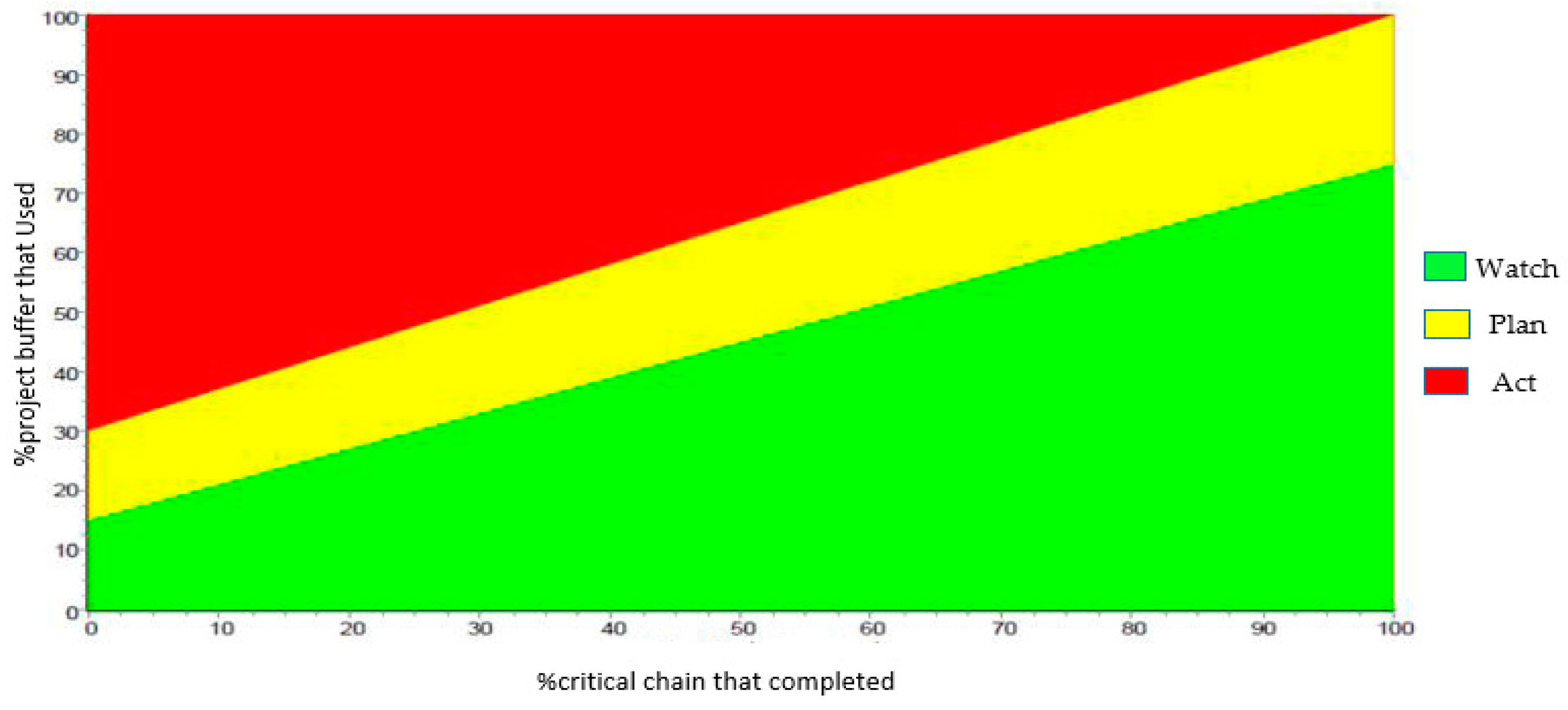
According to CCM, the project control is conducted using BM so that the buffers are divided into three equal parts, with each part accounting for 33% of the total buffer. The first part is green, the second is yellow, and the third is red. In each moment, no activity is necessary in the green part. The problem should be evaluated and corrective activities should be considered in the yellow part. Practice is required in the red part. In practice programs, the methods used for the immediate completion of unfinished activities in the chain, or those used to increase the speed of future activities in the chain, should be predicted. Project control is conducted, as shown in Figure 1 [35], to evaluate the rate of using a buffer proportional to the project development.
3. EVM/ES Method
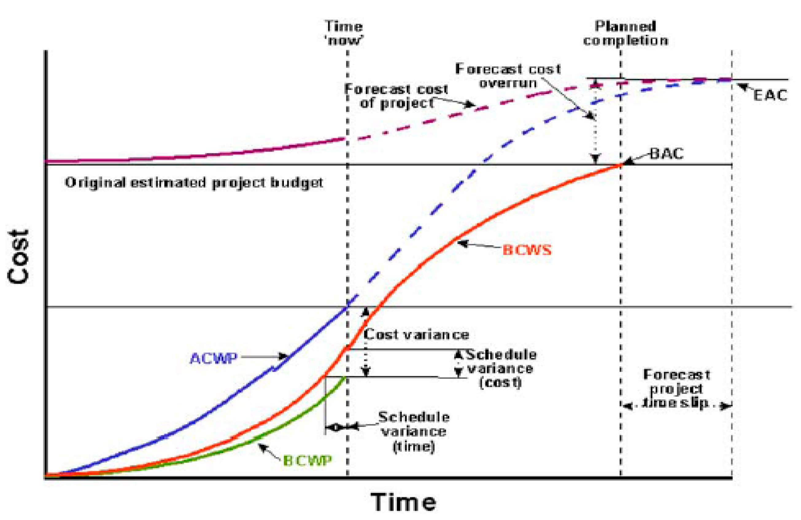
EVM is an important management technique used to evaluate the real development of a project or to conduct the comprehensive and integrated management of a project. According to EVM, project cost is an essential issue that should be addressed in project management, and the other issues should be considered in the next step. Today, authorities are mainly concerned with the comprehensive and correct cost management of a project, including resource planning, cost estimation, budgeting, and cost control. A baseline is required to apply EV. Currently, no other technique like EVM has been able to integrate the scope, cost, and scheduling of a project. Perhaps the main reason for applying EVM in different companies and industries is its ability to power manage a project using EVM to predict the final cost (probable) and the results of project scheduling. A project management team using the EVM can determine the cost and scheduling statuses of the project after a 15% development in the work scope agreed upon in the project contract. In clarifying the project status and problems, we cannot wait until we reach a 90% development before adopting a corrective action as we have no more time to perform and the project resources are mostly consumed. The EV sends a message to the project management to adopt an appropriate management action in which the immediate measures affect the results of the project in terms of cost and time. Through the EV, we can predict the required resources until the entire project is completed, and a new value called estimate at complete, which is greater than the budget at complete, is calculated statistically for the project. This concept is illustrated schematically in Figure 2 [36].
The abbreviations used in Figure 2 are defined as:
- ACWP: Actual cost of work performance
- BCWP: Budget cost of work performance
- BCWS: Budget cost of work schedule
- BAC: Budget at completion
- CPI: Cost performance index
- CV: Cost variance
- CV%: Cost variance percentage
- EAC: Estimate at completion
- SPI: Schedule performance index
- SV: Schedule variance
- SV%: Schedule variance percentage
- TCPI: To complete performance index
- VAC: Variance at completion.
To estimate the final cost and project scheduling results, we use CPI and SPI, which are derived from the EV. CPI connects the physical work value of the process to the real costs, which are directly paid for performing this work. If the amount of money paid is greater than the physical work performed, CPI will exhibit operational results exceeding the budget. Equation (2) shows how to calculate CV and CPI:
The second index is SPI. Along with SV calculation, it is addressed through Equation (3) and serves to predict the results of the project schedule. This index measures the performed work in the basic plan:
These two performance indices can be used separately or simultaneously to predict the results of the objective project exactly and rapidly. The cost management component of EVM is considered effective, but its schedule aspect has been questioned conceptually in the last few years. Only a few years ago, researchers and practitioners brought up issues on the use of EVM for schedule management [15]. Schedule variance and the schedule performance index should be used only as a warning mechanism and not as a real tool to analyze how the project is performing with regard to the schedule. Experts have criticized the behavior of SV and SPI indices over time and their interpretation in different aspects. The first criticism of the SPI index is its use of the financial unit rather than the time unit measures. Doing so makes the understanding of this index difficult and causes misrepresentation. The second criticism is that it cannot properly interpret the status of the project at a time when SV is equal to zero or SPI is equal to one because it can be interpreted in two ways: work has ended or work has gone according to plan. The third criticism is the behavior of SV and SPI at the end of the project. As the end of the project nears, SV, which always tends toward zero, and SPI, which tends toward one, converge. This outcome expresses the satisfactory performance of a project even if the project is delayed. To improve the performance of SPI, the earned schedule method converts the earned value at a given point in time into its equivalent duration (on the planned value graph) required to achieve that planned value. Figure 3 demonstrates this conversion on a conceptual EVM graph [15].
Using this approach, the method provides the earned schedule (ESt) for the project. Therefore, the earned schedule can be mathematically defined as adapted in Equation (4).
The corresponding duration from the beginning of the project until the status date is generally defined as actual time (AT) or elapsed time. We use the term actual duration (AD) in place of AT to maintain consistency and accuracy in this paper. The resultant EST is then compared with AD. Equation (5) shows how the earned schedule performance index (SPIt) is calculated:
4. Integrated Efficiency–Risk Methodology with the Combination of Two EVM and CCM Techniques
The main reason for combining the CCM and EVM methods is stated as follows:
In the CCM/BM method, which is obtained from TOC, time and time risks of the project are emphasized. As indicated in TOC, the system faces a limitation when developing. Time is the most important among the three main principles of management (i.e., time, cost, and performance). When time increases naturally, the consumed budget of the project also increases. To complete the project at a certain time, we usually have to interfere with the project scope. Therefore, we only apply time buffers in the project and ignore the cost items; the time buffers are considered the greatest constraint. Another limitation of this approach is the lack of formulas to estimate the duration and cost of the project. Note that many studies have been conducted to solve the constraints discussed in the previous sections, but they could not completely overcome these problems.
In the EVM/ES method, the emphasis is on project cost; the cost, value, and time control of the project are integrated in the method. This method is limited by the correlation between time and cost parameters, the lack of confidence in the SV and SPI compared with the CV and CPI, the lack of buffer time and cost, project risks, and the disregard for the path and critical chain of the project (i.e., what delays are related to what activities is not exactly determined). In other words, EVM/ES indices are applied based on cost without considering the impact time and are not related to path risk and the critical chain. Techniques to remove the correlation between the indices and the EDM methods, such as by combining the methods, fuzzy logic, and multivariate statistical analysis, have been used to solve some of the weaknesses of this method.
In the proposed hybrid efficiency-risk approach, the following basic steps are performed:
- Computing the cost and schedule buffers of the projects;
- The integration of the efficiency-risk control of the projects by managing the schedule and cost buffers;
- Estimating the cost and duration of the project completion with maximum accuracy and efficiency, including: estimating cost at completion (hybrid efficiency–risk approach); and estimating duration at completion (hybrid efficiency–risk approach).
4.1. Computing the Cost and Schedule Buffers of the Projects
In this method, it is necessary to compute the buffer mentioned in this article, the schedule buffer mentioned, and the cost buffer. For the calculation of these buffers, the estimated average time and cost for all activities are used. Based on the estimation of duration and cost of activities, the probability function of each one, and the formulas in Section 2, the cost buffer and schedule buffer of the project can be extracted by various methods.
4.2. The Integration of the Efficiency-Risk Control of the Projects by Managing the Schedule and Cost Buffers
Each buffer (schedule and cost) is divided into three equal parts of green, yellow, and red. The buffers can be in the green, yellow, or red zone in different stages of the project implementation based on progress and variance in terms of time and cost. Through the correct control of the usage of the two buffers in the project implementation (Table 2), the integration of the efficiency–risk control of the sustainable projects is conducted by managing the schedule buffer and the cost buffer [34].
Through Equations (6) and (7), the percentage of the cost buffer (PC) and that of the work done based on cost (WC) are calculated. The cost status of the project intersection of these two points is shown in Figure 4.
The percentage of the schedule buffer (PT) and that of the work done based on time (WT) are calculated using Equations (8) and (9). The duration status of the project intersection of two points is presented in Figure 4.
4.3. Estimating the Cost and Duration of Project Completion with Maximum Accuracy and Efficiency
The most important result of the hybrid efficiency–risk approach, with a combination of CCM/BM and EVM/ES in project control, is the estimated duration and cost at completion of the project considering maximum efficiency and reliability. By using the CCM technique in scheduling, the concepts of the EVM formulas to estimate cost at completion, the ES formulas to estimate the duration at completion, schedule buffer, and cost buffer, we offer new formulas to estimate the cost at completion and duration at completion of the project with maximum accuracy and efficiency return. The process is described below.
4.3.1. Estimate Cost at Completion (Hybrid Efficiency-Risk Approach)
Using the formulas provided in the EVM/ES and the buffers calculated in the previous section, the new formula estimate cost at completion with or without the cost buffer (hybrid efficiency-risk approach) is provided. Note that the EVM technique in project cost-control works with complete accuracy. Through the formulas and concepts of the CCM/BM technique, new formulas are provided at this stage.
- BPVi: Baseline planned value of the scheduled activity i, and the authorized budget assigned to the work to be accomplished for activity i. BPVi is independent of the status date. Some may refer to it the baseline cost for activity i.
- BCAC0: Budget cost at completion, regardless of the cost buffer for the project, is the sum of BPVi for all the planned activities at the baseline plan, which is calculated using Equation (10):
- BCAC: Budget cost at completion with regard to the cost buffer (combination of performance and risk parameters), which is calculated using Equation (11):
- BC: Cost buffer percent of BCAC0, which is calculated using Equation (12):
- PC: The percentage of the cost buffer is calculated with the help of the Equation (6).
- WC: The percentage of work done based on cost, which is calculated using Equation (7).
- CPI: Based on parameters BCAC0, WC, PC, cost buffer, and formulas presented in Section 3 (EVM/ES), the cost performance index can be calculated as Equation (13). The index is used to update the remainder of the cost buffer:
- ECAC0: In the phases of project control, estimated cost at completion, regardless of the cost buffer, and only after the control of the project buffer usage is done. In other words, with the help of the cost buffer usage, the adjusted BCAC0 is estimated, which is the same as ECAC0. Equation (14) calculates this value:
- CBA: Cost buffer, which is adjusted during the phases of project control, with the help of the percentages of the cost buffer (PC) and cost performance index (CPI) parameters for calculating the adjusted cost buffer, using Equation (15).
- ECAC: Estimated cost at completion, with regard to cost buffers (combination of performance and risk parameters), is calculated using Equation (16):
4.3.2. Estimate Duration at Completion (Hybrid Efficiency–Risk Approach)
Using the formulas in EVM/ES for calculating the buffers in the previous section, a new formula to estimate duration at completion that considers the buffers (hybrid efficiency-risk approach) is presented. As the EVM techniques in the project control duration does not work with complete accuracy, new formulas are developed using the ES techniques and CCM/BM concepts at this stage.
- BPD0: The baseline planned duration, regardless of the schedule buffer, of the project is the authorized duration assigned to the scheduled work to be accomplished for the entire project irrespective of the status date.
- BPD: Total baseline planned duration, with regard to the schedule buffer (combination of performance and risk parameters), which is calculated using Equation (17):
- BT: Schedule buffer percent of BPD0, which is calculated using Equation (18):
- PT: The percentage of the schedule buffer is calculated with the help of Equation (19):
- WT: The percentage of work done based on time, which is calculated using Equation (20):
- SPIT: With the help of the parameters of BPD0, WT, PT, Schedule Buffer, and formulas presented in EVM/ES, the schedule performance index can be calculated as follows: The SPIT is used to update the remaining schedule buffer, which can be seen in Equation (21):
- EDAC0: Within the phases of project control, the estimated duration at completion, regardless of the schedule buffer, and only after the control of project buffer usage is done. In other words, with the help of schedule buffer usage, the adjusted BPD0 is estimated, which is the same as EDAC0. Equation (22) calculates this value:
- SBA: Adjusted schedule buffer; during the phases of project control, with the help of the percentage of the schedule buffer (PT) and the schedule performance index (SPI) parameters, the calculation of the adjusted schedule buffer uses Equation (23):
- EDAC: Estimated duration at completion, with regard to schedule buffers (the combination of performance and risk parameters), which is calculated using Equation (24).
5. Case Study
Mobarakeh Steel Co. is a leading Iranian company that produces steel sheets. This company is committed to playing a central role in the industrial, economic, and social development of the country, to improving its technologies in the steel industry, and to acting as an international organization that produces about 50% of the country’s steel for use in industries, such as automobiles, energy, heavy steel, fluid transfer tubes, packaging, electricity, profile, and tube. This company comprises seven industrial complexes distributed across the country and has more than 20,000 employees in its different departments. One of the projects related to this plant is the development of a custom product, which is used as a case study for applying the proposed approach of integrated risk–efficiency methodology. The Primavera Risk Analysis software version 8.7 (Oracle Corporation, Redwood City, CA, USA) is used for the application. The project is composed of three parts, with each part built separately and then assembled. The project activities, activity duration, and costs required are extracted, as shown in Table 3. Cut and paste, error root square, and Monte Carlo simulation are used to calculate the schedule and cost buffer of the projects. The duration and costs are estimated as a probability (triangular probability distribution).
After scheduling the project, the baseline planned duration (BPD0) is estimated to be equal to 48 days, and the budget cost at completion regardless of the buffer cost (BAC0) is calculated using Equation (25):
The results of the deterministic scheduling are illustrated in Figure 5.
Based on the equations in Section 2, the schedule and cost buffer are calculated by cut and paste, error root square, and Monte Carlo simulation as Equations (26) and (27). Based on the calculations, the results of the error root square are obtained:
The project in two control periods of 15 and 30 days is updated and monitored. In the mentioned periods all activities, except no. 130 (related to the test activity of part 3), are conducted based on a scheduling plan. Using the proposed methodology of integrated risk–efficiency methodology, the duration progress, cost progress, usage percentage of the schedule, and cost buffer are calculated using Equations (28) and (29):
The duration and cost at completion of the project in the two control periods of 15 and 30 days are also estimated using the proposed methodology.
- BCAC: Budget cost at completion with regard to the cost buffer (combination of performance and risk parameters), which is calculated using Equation (30):
- BC: Cost buffer percentage of BCAC0, which is calculated using Equation (31):
- ECAC0: During the phases of project control, estimated cost at completion, regardless of the cost buffer, and only after control of project buffer usage is done. In other words, with the help of cost buffer usage, the adjusted BCAC0 is estimated, which is the same as ECAC0. Equation (32) calculates this value:
- ECAC: Estimated cost at completion with regard to cost buffers (combination of performance and risk parameters), which is calculated using Equation (33);
- BPD: Total baseline planned duration, with regard to the schedule buffer (combination of performance and risk parameters), which is calculated using Equation (34):
- BT: Schedule buffer percentage of BPD0 which is calculated using Equation (35):
- EDAC0: Within the phases of project control, the estimated duration at completion, regardless of the buffer, and only after control of project buffer usage is done. In other words, with the help of schedule buffer usage, the adjusted BPD0 is estimated, which is the same as EDAC0. Equation (36) calculates this value:
- EDAC: Estimated duration at completion with regard to schedule buffers (the combination of performance and risk parameters), which is calculated using Equation (37):
6. Results and Conclusions
Most of the project control techniques non-uniformly focus on the qualitative (risk) and quantitative (time and cost) parameters. Among them, CCM/BM and EVM/ES are two new scientific techniques proposed in project management, and they both have advantages and disadvantages. The CCM/BM method is derived from limitations theories and focuses on the time of the project time discussion. To complete a project at the certain time, we usually have to interfere with the project scope. Therefore, we apply only scheduling buffers in the project and disregard the cost items; this is the greatest limitation of the method. Another main constraint of this approach is its failure to provide accurate charts and formulas for control, estimated duration, and cost at completion of the project.
The EVM/ES method emphasizes the project cost, and it integrates the cost, value, and time control of the project. This method is limited by the correlation between time and cost parameters, the lack of confidence in the SV and SPI compared with the CV and CPI, the lack of usage of buffer time and cost, project risks, and the disregard for the path and the critical chain of the project (whether delays are related to what activities is not exactly determined). In other words, the EVM/ES indices are applied based on cost without considering the impact time, and they are not related to path risk and the critical chain. In this method, the unique advantages of CCM/BM, such as the focus on the critical chain instead of the critical path, prevention of confidence time for each activity, avoidance of student syndrome, and the lack of concurrent tasks, are not used.
Investigation on CCM/BM demonstrates a superior focus on time parameter and time-based risks in a concurrent manner and on the other hand, the key advantage of EVM/ES is to concentrate on cost parameters thereby establishing equations for EDAC and ECAC. As such, integration of the above techniques leads to developing a framework incorporating the above advantages all in one which suits the needs of applied control on sustainable projects by taking into consideration quantitative parameters (time and cost), as well as qualitative parameters (risk).
In the integrated risk–efficiency methodology, we use the CCM/BM method by combining the CCM/BM and EVM/ES techniques. We include one cost buffer in our calculations aside from the schedule buffer. We perform simultaneous management of the schedule and cost of project by correcting the control of these two buffers. By using the formulas and concepts of EVM/ES in the estimated duration and cost at completion, new formulations are developed with maximum accuracy and efficiency through buffer management.
More precisely, two recently-developed techniques, known as CCM/BM and EVM/ES, have attracted considerable attention while each one has its own disadvantages. In the case of CCM/BM, the main limitation is a dominant focus on time and paying no attention to cost and related risks which cannot bring illustrative equations of EDAC and ECAC with respect to the project development. On the other hand, EVM/ES fails to consider the time parameter comparing to cost, time risks, and cost risk. According to this background, the proposed methodology eliminates the above limitations attributed to either CCM/BM or EVM/ES. The integrated technique exerts a significant importance on the cost parameter, as well as time parameters in a risk–efficiency approach. Correspondingly, the cost buffer is added to the time buffer, leading to control the whole time and of the cost risks associated to a project. Meanwhile, equations of EDAC and ECAC are derived similar to relations given on EVM/ES with respect to project progress, and time and cost buffers. In brief, the following are the most important advantages resulting from the integrated approach:
- Taking full advantages of CCM/BM (allocating precaution time to the whole project and not to each individual activity, preventing the occurrence of Student Syndrome and parallel activities) and EVM/ES (concurrent control on time and cost, thereby drawing equations for ECAC and EDAC);
- Integrated control on the efficiency (time and cost) and risk of projects;
- Calculation of time and cost buffers to deal with cost and time risks;
- Providing a tight control (fast and accurate) on time, cost, and related risks with the help of developed buffers;
- Giving an estimation on EDAC and ECAC with respect to the percentage of project progress, as well as the consumed time–cost buffers;
- Providing an applied procedure to implement the methodology in practice.
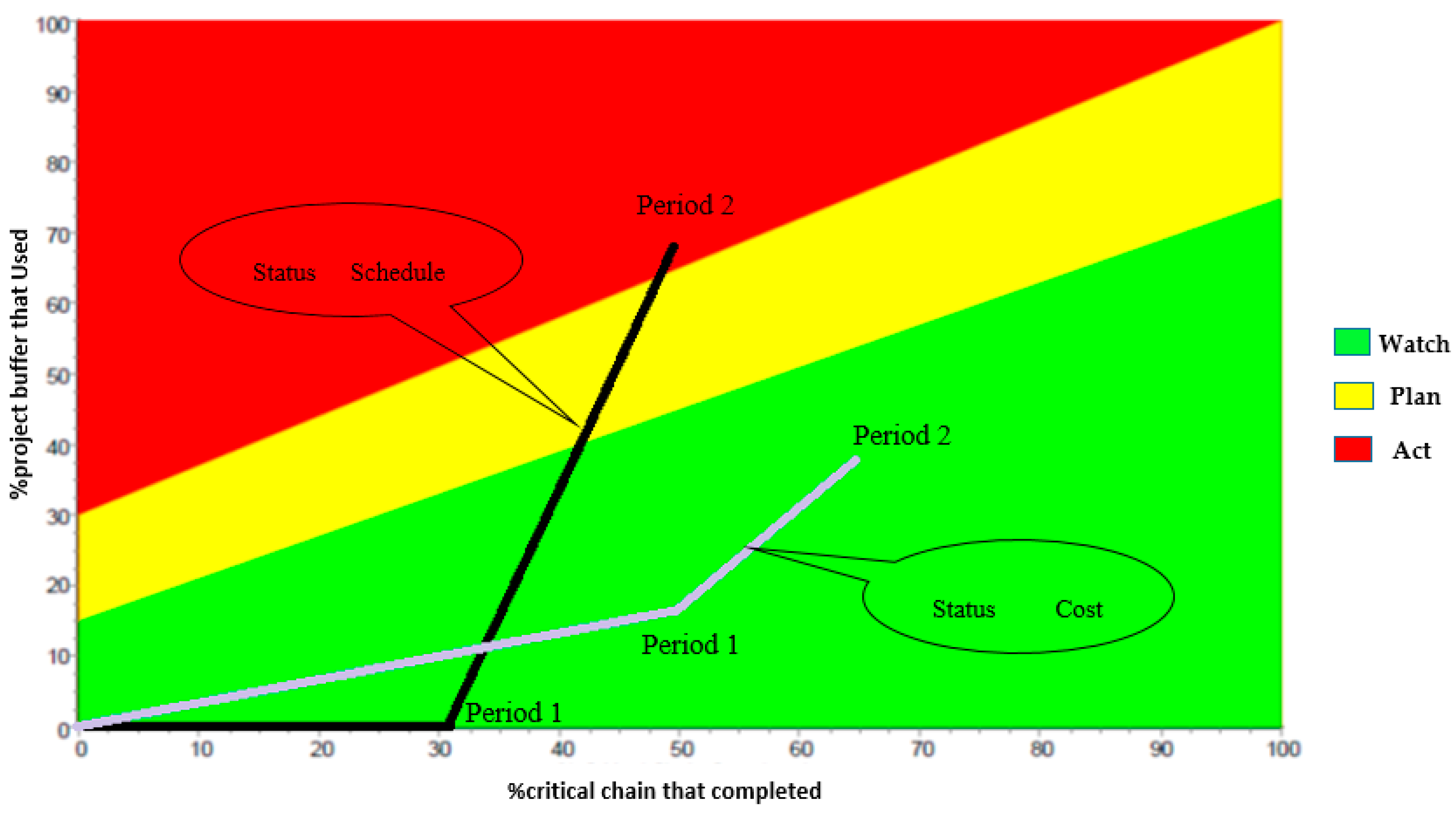
Based on the analysis of the obtained results from the case study, the buffer is in the green zone in terms of cost and schedule buffers in the control period of 15 days. As shown in Table 2, the proposed method does not require special action. In the control period of 30 days, the buffer is in the yellow zone in terms of cost and in the red zone in terms of schedule. In the proposed method, the speed of the project implementation should be increased without extra cost by using new techniques (Table 2). Figure 6 plots the value of the project progress and usage percent of the buffer in two control periods. Note that, with regard to cost and duration progress, the duration and cost variance of the project are in the green zone in the control period of 15 days. The duration variance is in the red zone and the cost variance is in the green zone in the control period of 30 days.
The estimate cost at completion in the first period is equal to $200,841 and that in the second period is equal to $232,983, because of the delays occurring in the control periods. In addition, the estimate duration at completion in the first period is equal to 61 days and that in the second period is equal to 93 days.
By applying the proposed technique to a case study, the results show that, in two time periods of 15 and 30 days and the percentages of time–cost buffers consumed, an integrated control of the quantitative parameters and risks are well achieved and, subsequently, necessary actions to be taken in each period are addressed in Table 2. Above all, a good estimation of EDAC and ECAC are provided.
The present article contributes to further research by using single or multivariate statistical control charts to accurately monitor the buffers and present the integrated risk–efficiency methodology in the controlling program and project portfolio.
Data Availability Statements
All data generated or analyzed during the study are included in the published paper. However, crude data are available as per request (via email to the corresponding author).
Acknowledgments
The authors are grateful to the anonymous reviewers who provided useful comments on an earlier draft of the paper.
Author Contributions
M.S.G. and V.G. have contributed materially to the paper, including: (1) making substantial contributions to conception and design, acquisition of data, and analysis and interpretation of data; (2) participating in drafting the article or revising it critically for important intellectual content; and (3) giving final approval of the version to be submitted and any revised version. Furthermore, S.R. and A.M. can be considered as participating investigators, and in accordance with their functions and contributions, they have served as scientific advisors. Also, they had a key role in the revision process by preparing some details of the algorithms in some new Section 4.3, Section 4.3.1 and Section 4.3.2. Moreover, they kindly investigated new results in Section 6.
Conflicts of Interest
Authors confirm that this article is the original work of the authors and have no conflict of interest to declare. Moreover, there is no founding sponsor which had any role in the design of the study; in the collection, analyses, or interpretation of data; in the writing of the manuscript; and in the decision to publish the results.
References
- Snyder, C.S. A Guide to the Project Management Body of Knowledge: PMBOK(®) Guide; Project Management Institute: Newtown Square, PA, USA, 2014. [Google Scholar]
- Calderon-Monge, E.; Pastor-Sanz, I.; Huerta-Zavala, P. Economic Sustainability in Franchising: A Model to Predict Franchisor Success or Failure. Sustainability 2017, 9, 1419. [Google Scholar] [CrossRef]
- Vanhoucke, M.; Vandevoorde, S. A simulation and evaluation of earned value metrics to forecast the project duration. J. Oper. Res. Soc. 2007, 58, 1361–1374. [Google Scholar] [CrossRef]
- Marshall, R. A Quantitative Study of the Contribution of Earned Value Management to Project Success on External Projects under Contract; Lille Graduate School of Management: Lille, France, 2007. [Google Scholar]
- Chou, J.-S.; Chen, H.-M.; Hou, C.-C.; Lin, C.-W. Visualized EVM system for assessing project performance. Autom. Constr. 2010, 19, 596–607. [Google Scholar] [CrossRef]
- Kim, B.-C.; Reinschmidt, K.F. Probabilistic forecasting of project duration using Kalman filter and the earned value method. J. Constr. Eng. Manag. 2010, 136, 834–843. [Google Scholar] [CrossRef]
- XIE, X.-M.; Guang, Y.; Chuang, L. Software development projects IRSE buffer settings and simulation based on critical chain. J. China Univ. Posts Telecommun. 2010, 17, 100–106. [Google Scholar] [CrossRef]
- Czarnigowska, A.; Jaskowski, P.; Biruk, S. Project performance reporting and prediction: Extensions of Earned value management. Int. J. Bus. Manag. Stud. 2011, 1, 11–20. [Google Scholar]
- Naeni, L.M.; Shadrokh, S.; Salehipour, A. A fuzzy approach for the earned value management. Int. J. Proj. Manag. 2011, 29, 764–772. [Google Scholar] [CrossRef]
- Hanna, A.S. Using the earned value management system to improve electrical project control. J. Constr. Eng. Manag. 2011, 138, 449–457. [Google Scholar] [CrossRef]
- Acebes, F.; Pajares, J.; Galán, J.M.; López-Paredes, A. Beyond earned value management: A graphical framework for integrated cost, schedule and risk monitoring. Procedia Soc. Behav. Sci. 2013, 74, 181–189. [Google Scholar] [CrossRef]
- Elshaer, R. Impact of sensitivity information on the prediction of project’s duration using earned schedule method. Int. J. Proj. Manag. 2013, 31, 579–588. [Google Scholar] [CrossRef]
- Vanhoucke, M.; Colin, J. On the use of multivariate regression methods for longest path calculations from earned value management observations. Omega 2016, 61, 127–140. [Google Scholar] [CrossRef]
- Lipke, W. Earned Schedule-Ten Years After. In The Measurable News (3); Walt Lipke, PMI®: Oklahoma City, OK, USA, 2013; pp. 15–21. [Google Scholar]
- Khamooshi, H.; Golafshani, H. EDM: Earned Duration Management, a new approach to schedule performance management and measurement. Int. J. Proj. Manag. 2014, 32, 1019–1041. [Google Scholar] [CrossRef]
- Chen, H.L. Improving forecasting accuracy of project earned value metrics: Linear modeling approach. J. Manag. Eng. 2014, 30, 135–145. [Google Scholar] [CrossRef]
- Colin, J.; Vanhoucke, M. Setting tolerance limits for statistical project control using earned value management. Omega 2014, 49, 107–122. [Google Scholar] [CrossRef] [Green Version]
- Wang, W.-X.; Wang, X.; Ge, X.-l.; Deng, L. Multi-objective optimization model for multi-project scheduling on critical chain. Adv. Eng. Softw. 2014, 68, 33–39. [Google Scholar] [CrossRef]
- Yang, S.; Fu, L. Critical chain and evidence reasoning applied to multi-project resource schedule in automobile R&D process. Int. J. Proj. Manag. 2014, 32, 166–177. [Google Scholar]
- Peng, W.; Huang, M. A critical chain project scheduling method based on a differential evolution algorithm. Int. J. Prod. Res. 2014, 52, 3940–3949. [Google Scholar] [CrossRef]
- Ma, G.; Wang, A.; Li, N.; Gu, L. Improved critical chain project management framework for scheduling construction projects. J. Constr. Eng. Manag. 2014, 140, 04014055. [Google Scholar] [CrossRef]
- Acebes, F.; Pereda, M.; Poza, D.; Pajares, J.; Galán, J.M. Stochastic earned value analysis using Monte Carlo simulation and statistical learning techniques. Int. J. Proj. Manag. 2015, 33, 1597–1609. [Google Scholar] [CrossRef]
- Willems, L.L.; Vanhoucke, M. Classification of articles and journals on project control and earned value management. Int. J. Proj. Manag. 2015, 33, 1610–1634. [Google Scholar] [CrossRef]
- Ghaffari, M.; Emsley, M.W. Current status and future potential of the research on Critical Chain Project Management. Surv. Oper. Res. Manag. Sci. 2015, 20, 43–54. [Google Scholar] [CrossRef]
- Batselier, J.; Vanhoucke, M. Evaluation of deterministic state-of-the-art forecasting approaches for project duration based on earned value management. Int. J. Proj. Manag. 2015, 33, 1588–1596. [Google Scholar] [CrossRef]
- Colin, J.; Martens, A.; Vanhoucke, M.; Wauters, M. A multivariate approach for top-down project control using earned value management. Decis. Support Syst. 2015, 79, 65–76. [Google Scholar] [CrossRef]
- Chen, H.L.; Chen, W.T.; Lin, Y.L. Earned value project management: Improving the predictive power of planned value. Int. J. Proj. Manag. 2016, 34, 22–29. [Google Scholar] [CrossRef]
- Sarkar, D.; Babu, R. Applications of Critical Chain Project Management and Buffer Sizing for Elevated Corridor Metro Rail Project. Constraints 2016, 3. [Google Scholar] [CrossRef]
- Zhang, J.; Song, X.; Díaz, E. Project buffer sizing of a critical chain based on comprehensive resource tightness. Eur. J. Oper. Res. 2016, 248, 174–182. [Google Scholar] [CrossRef]
- Wei, N.-C.; Bao, C.-P.; Yao, S.-Y.; Wang, P.-S. Earned Value Management Views on Improving Performance of Engineering Project Management. Int. J. Org. Innov. 2016, 8, 93–111. [Google Scholar]
- Rodriguez, J.C.M.; et al. An Overview of Earned Value Management in Airspace Industry. In Proceedings of the Tenth International Conference on Management Science and Engineering Management, Baku, Azerbaijan, 30 August–2 September 2016. [Google Scholar]
- Goldratt, E. Theory of Constraints (TOC); North River Press: Croton-on-Hudson, NY, USA, 1990. [Google Scholar]
- Patrick, F.S.t. Critical chain and risk management—Protecting project value from uncertainty. World Proj. Manag. Week 2002. [Google Scholar]
- Tukel, O.I.; Rom, W.O.; Eksioglu, S.D. An investigation of buffer sizing techniques in critical chain scheduling. Eur. J. Oper. Res. 2006, 172, 401–416. [Google Scholar] [CrossRef]
- Leach, L.P. Critical Chain Project Management; Artech House: Norwood, MA, USA, 2014. [Google Scholar]
- Fleming, Q.W.; Koppelman, J.M. Earned Value Project Management; Project Management Institute: Newtown Square, PA, USA, 2005. [Google Scholar]
Figure 1.
Project control charts based on project progress and the buffer usage percentage.
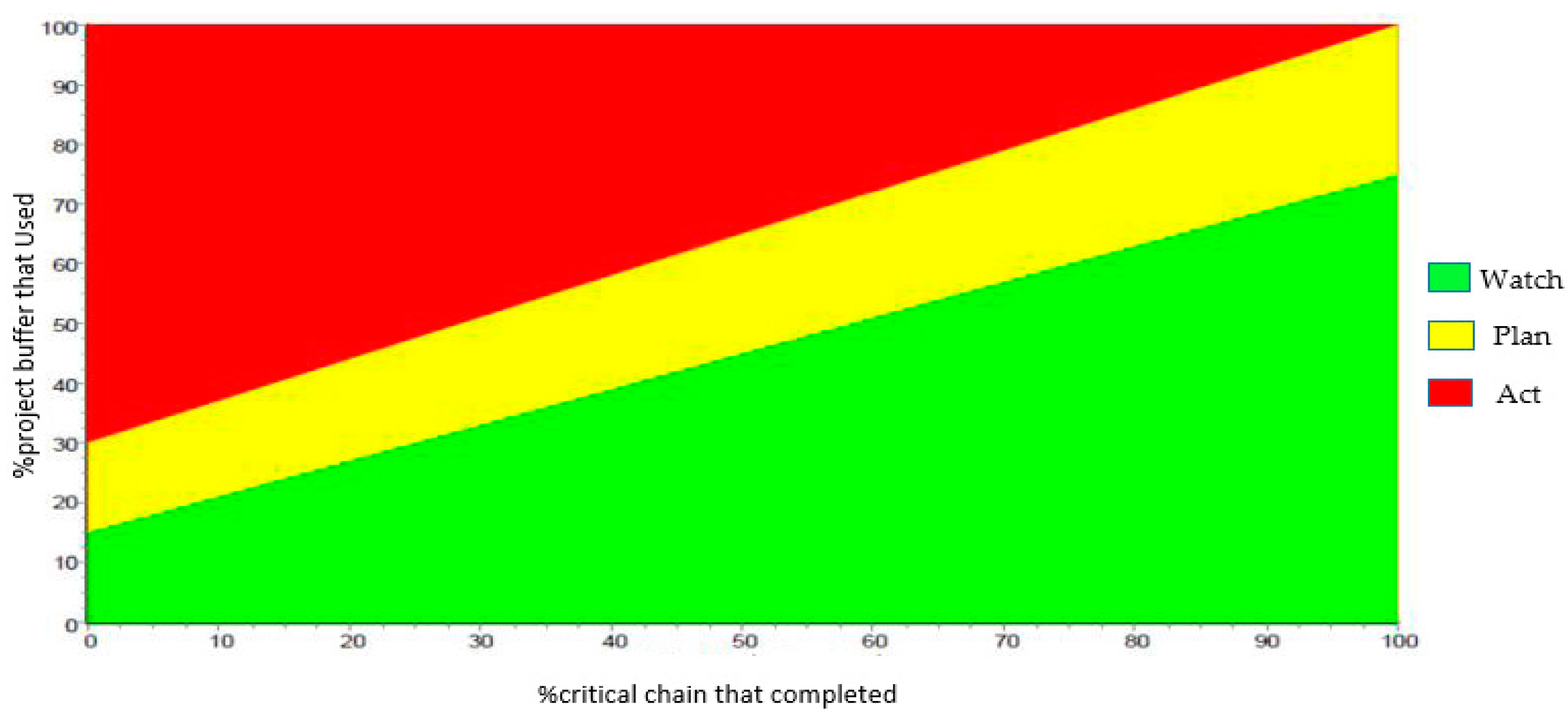
Figure 2.
Method of calculation of budget at completion (BAC) and estimate at completion (EAC) values [36].
Figure 2.
Method of calculation of budget at completion (BAC) and estimate at completion (EAC) values [36].

Figure 3.
Method of calculating the earned schedule [15].
Figure 3.
Method of calculating the earned schedule [15].
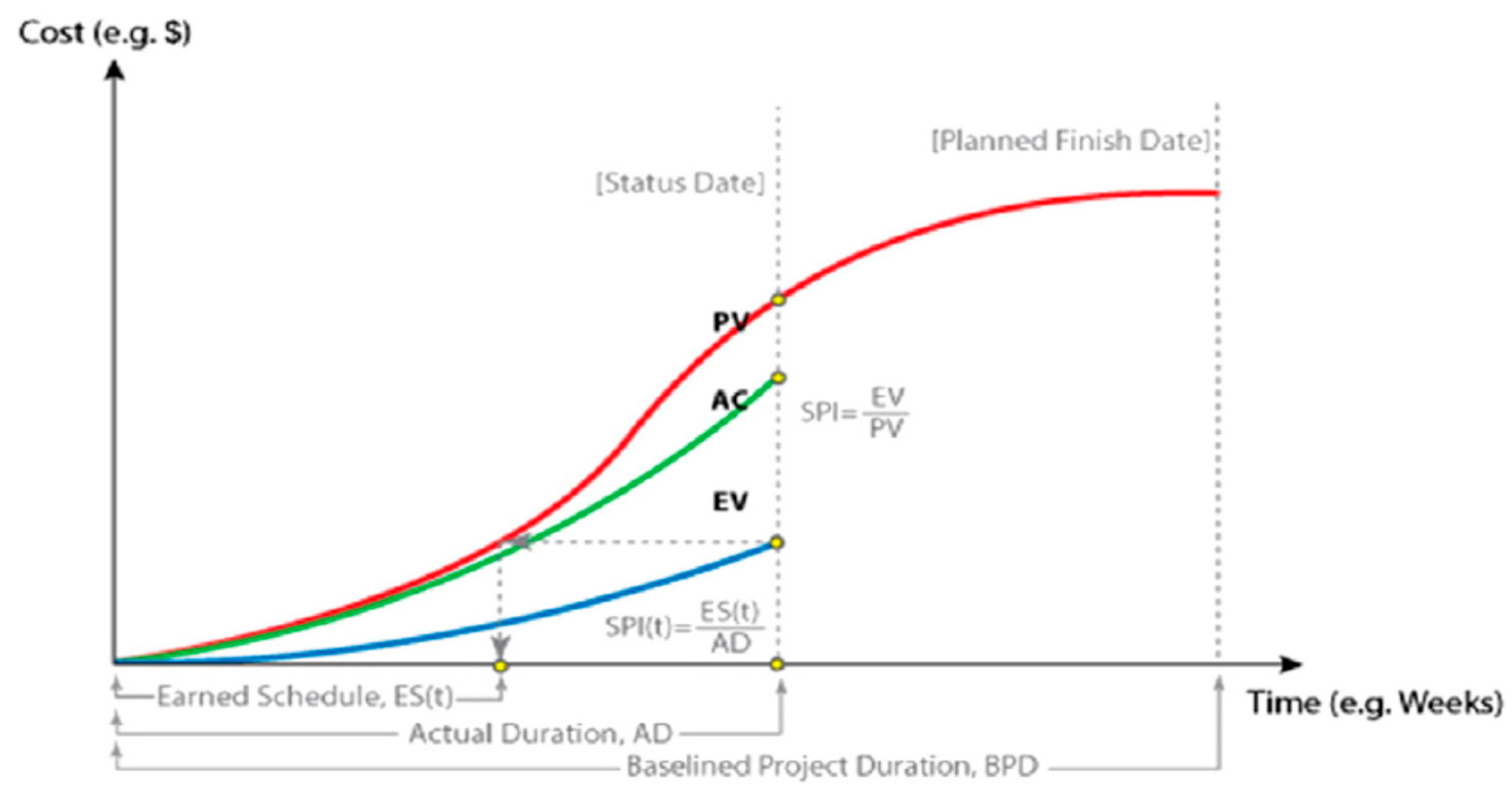
Figure 4.
Project control charts based on project progress (schedule or cost) and the buffer usage percent (schedule or cost).
Figure 4.
Project control charts based on project progress (schedule or cost) and the buffer usage percent (schedule or cost).

Figure 5.
Deterministic scheduling.
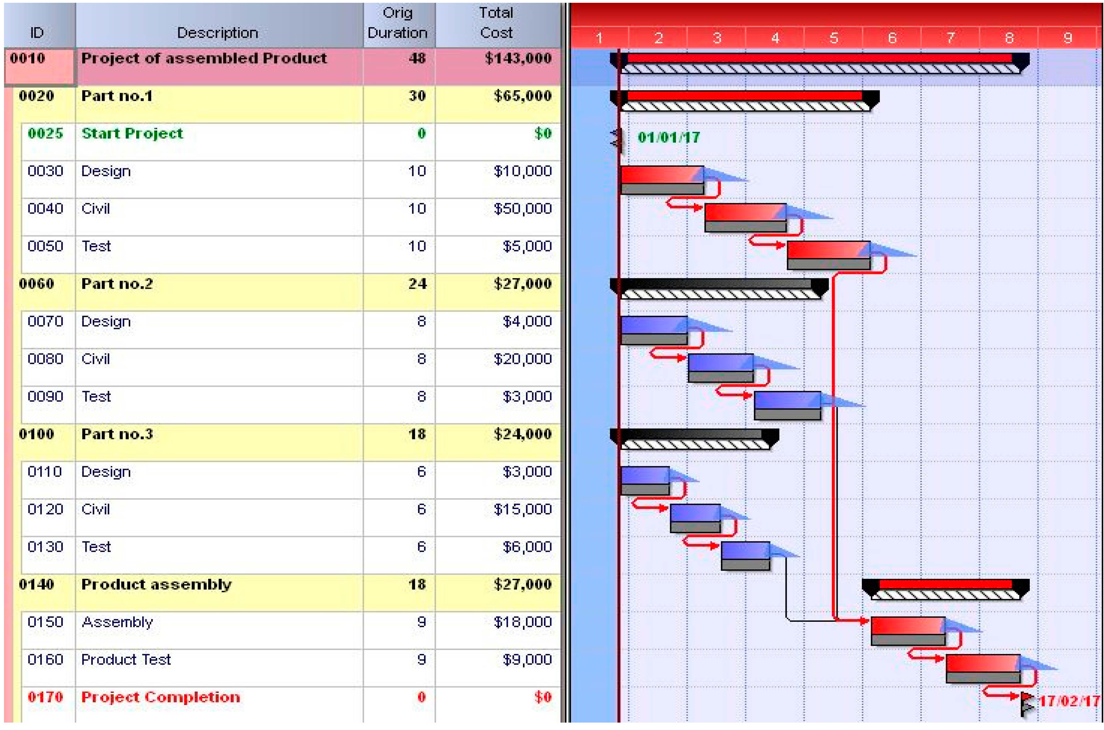
Figure 6.
Case study project status based on project progress and the buffer usage percent (cost and schedule).
Figure 6.
Case study project status based on project progress and the buffer usage percent (cost and schedule).


Table 1.
Research taxonomy of control project methods based on the critical chain method (CCM) and earned value management (EVM).
Table 1.
Research taxonomy of control project methods based on the critical chain method (CCM) and earned value management (EVM).
| Estimated Cost at Completion | Estimated Duration at Completion | CCM Advantages | Capability Uncertainty | Performance in Schedule Control | Performance in Cost Control | Method Name | Publication |
|---|---|---|---|---|---|---|---|
| √ | − | − | − | − | √ | Earned value project management | Vanhoucke and Vandevoorde (2007) [3] |
| √ | − | − | √ | − | √ | Fuzzy approach for earned value management | Naeni et al. (2011) [9] |
| √ | − | − | √ | − | √ | A graphical framework for EVM | Acebes et al., 2013 [11] |
| − | − | √ | √ | √ | − | Improved critical chain project management | Ma et al., 2014 [21] |
| √ | √ | − | − | √ | √ | Earned duration management | Khamooshi and Golafshani (2014) [15] |
| − | − | √ | √ | √ | − | Critical chain based on comprehensive resource tightness | Zhang et al., 2016 [29] |
| √ | √ | √ | √ | √ | √ | Efficiency–risk approach | Current study |
Table 2.
Project management by schedule and cost buffer.
| Cost Buffer | ||||
|---|---|---|---|---|
| Green | Yellow | Red | ||
| Follow schedule more quickly even if it leads to spending more cost. | Without extra cost, increase speed of project implementation by using of new techniques. | Follows more quickly and do non-critical activities in a cost saving manner. | Red | Schedule Buffer |
| Attention should be paid to the control of the project duration and it is not necessary to make corrective actions. | At remaining of project, continue same status of time and cost. | Keep speed in implementation of work with saving cost on noncritical activities. | Yellow | |
| Do not need to make corrective actions. | Attention should be paid to the control of the project cost and it is not necessary to make corrective actions. | As far as possible, the value of the project is preserved and the costs are saved. | Green | |
Table 3.
Activity list, duration, and budget cost of project.
| ID | Activity Name | Expected Duration | Expected Cost | ||||
|---|---|---|---|---|---|---|---|
| Description | Min Duration (days) | Most Likely (days) | Max Duration (days) | Min Cost ($) | Most Likely Cost ($) | Max Cost ($) | |
| 0010 | Project of assembled product | 116,250 | 143,000 | 233,060 | |||
| 0020 | Part No. 1 | 52,000 | 65,000 | 104,000 | |||
| 0025 | Start project | Milestone | - | ||||
| 0030 | Design | 8 | 10 | 16 | 8000 | 10,000 | 16,000 |
| 0040 | Civil | 8 | 10 | 16 | 40,000 | 50,000 | 80,000 |
| 0050 | Test | 8 | 10 | 16 | 4000 | 5000 | 8000 |
| 0060 | Part No. 2 | 20,250 | 27,000 | 47,250 | |||
| 0070 | Design | 6 | 8 | 14 | 3000 | 4000 | 7000 |
| 0080 | Civil | 6 | 8 | 14 | 15,000 | 20,000 | 35,000 |
| 0090 | Test | 6 | 8 | 14 | 2250 | 3000 | 5250 |
| 0100 | Part No. 3 | 20,000 | 24,000 | 39,860 | |||
| 0110 | Design | 5 | 6 | 10 | 2500 | 3000 | 5000 |
| 0120 | Civil | 5 | 6 | 10 | 12,500 | 15,000 | 24,900 |
| 0130 | Test | 5 | 6 | 10 | 5000 | 6000 | 9960 |
| 0140 | Product Assembly | 24,000 | 27,000 | 41,950 | |||
| 0150 | Assembly | 8 | 9 | 14 | 16,000 | 18,000 | 28,000 |
| 0160 | Product test | 5 | 6 | 10 | 8000 | 9000 | 13,950 |
| 0170 | Project completion | Milestone | - | ||||
© 2017 by the authors. Licensee MDPI, Basel, Switzerland. This article is an open access article distributed under the terms and conditions of the Creative Commons Attribution (CC BY) license (http://creativecommons.org/licenses/by/4.0/).
Share and Cite
MDPI and ACS Style
Ghazvini, M.S.; Ghezavati, V.; Raissi, S.; Makui, A. An Integrated Efficiency–Risk Approach in Sustainable Project Control. Sustainability 2017, 9, 1575. https://doi.org/10.3390/su9091575
AMA Style
Ghazvini MS, Ghezavati V, Raissi S, Makui A. An Integrated Efficiency–Risk Approach in Sustainable Project Control. Sustainability. 2017; 9(9):1575. https://doi.org/10.3390/su9091575
Chicago/Turabian StyleGhazvini, Mohammadreza Sharifi, Vahidreza Ghezavati, Sadigh Raissi, and Ahmad Makui. 2017. "An Integrated Efficiency–Risk Approach in Sustainable Project Control" Sustainability 9, no. 9: 1575. https://doi.org/10.3390/su9091575
Note that from the first issue of 2016, this journal uses article numbers instead of page numbers. See further details here.