Uncertainties of Two Methods in Selecting Priority Areas for Protecting Soil Conservation Service at Regional Scale


1
School of Geography and Tourism, Shaanxi Normal University, Xi’an 710119, Shaanxi, China
2
State Key Laboratory of Urban and Regional Ecology, Research Center for Eco-Environmental Sciences, Chinese Academy of Sciences, Beijing 100085, China
3
Key Laboratory of Digital Earth Science, Institute of Remote Sensing and Digital Earth, Chinese Academy of Sciences, Beijing 1000101, China
*
Author to whom correspondence should be addressed.
Sustainability 2017, 9(9), 1577; https://doi.org/10.3390/su9091577
Submission received: 10 August 2017
/
Revised: 30 August 2017
/
Accepted: 1 September 2017
/
Published: 7 September 2017
Abstract
:Soil conservation (SC) is an important ecosystem regulating service. At present, methods for SC mapping to identify priority areas are primarily based on empirical soil erosion models, such as the RUSLE (Revised Universal Soil Loss Equation) based model. However, the parameters of the empirical soil conservation model are based on long-term observations of field experiments at small spatial scales, which are very difficult to obtain and must be simplified when implementing these models at large spatial scales. Such simplification of model parameters may lead to uncertainty in quantifying SC at regional scale. In this study, we have analyzed a new method to map SC in Jiangxi Province of China based on the multiplication of multiple biophysical data. After comparing the spatial-temporal changes of SC from the RUSLE based model and those from the surrogate indicator based method in the study area, the similarities and differences of these methods for identifying SC priority areas were revealed. The result showed that the two methods similarly represented the effects of vegetation coverage and land use types on SC, however, they were significantly different in representing the spatial pattern of SC priority areas and its temporal change. Based on the comparisons, the advantages and drawbacks for both methods were made clear and suggestions were made for the suitable use of the two methods, which may benefit for the research and application of concerning the planning and assessment with SC as key criteria.
1. Introduction
Spatial conservation prioritization is a form of conservation assessment that supports conservation planning and is the key technical phase within the systematic conservation planning process; it aims to answer questions about when, where, and how conservation goals can efficiently be achieved [1,2,3]. Traditionally, conservationists have focused on the conservation of biodiversity to make systematic conservation planning [4,5]. Recently, many conservationists have begun focusing on both the conservation of biodiversity and the sustainable provision of ecosystem services (ESs), which are the benefits that humans obtain from ecosystems that support the well-being of humans [6,7,8,9]. However, the goal of conserving both biodiversity and ESs is less likely to be achieved unless the target types of ESs have been spatially explicitly mapped [7,8,10,11]. Spatially explicit mapping of ESs is one of the critical methods of mainstreaming ESs into spatial conservation prioritization in systematic conservation planning that focuses on planning implementation and conservation monitoring [10,12,13]. In addition, spatially explicit mapping of priority areas for ESs is an essential step of incorporating ESs into policies and practices to ensure the continuous provision of ESs and associated benefits to humans [10,14,15,16,17].
The SC refers to the integrative capability of terrestrial ecosystems and their vegetation cover, root matrix, and soil biota to prevent soil damage from erosion/siltation [18], which is an important ecosystem regulating service [6]. The worldwide degradation of ecosystem SC exacerbates serious soil erosion problems [19] and has become a concern of stakeholders and decision-makers during the conservation planning process. Recently, the degradation of terrestrial ecosystem SC of China has resulted in serious soil erosion, which has become one of the most critical national ecological problems; in fact, nearly one-third of China’s land area suffers from soil erosion, resulting in severe economic losses in China. Therefore, a robust method should be provided to mapping ecosystem SC in order to conserving ecosystem SC and release the damage of soil erosion. At present, methods for spatially explicit mapping of the SC of terrestrial ecosystems are primarily based on empirical soil erosion models, such as the RUSLE [17,20,21,22]. Based on the empirical models, the SC can be quantified by determining the difference between the actual soil loss of the landscape and the potential soil loss, which presumes no vegetation cover in an extremely degraded form of the landscape [21,23]. However, this hypothesis may yield a considerable overestimation of SC. More importantly, the parameters of the empirical soil conservation model are based on long-term observations of field experiments at small spatial scales, which are very difficult to obtain and must be simplified when implementing these models at large spatial scales. Such simplification of model parameters may lead to uncertainty in quantifying SC at large spatial scales [24]. Recently, Carreño et al. [25] formulated a simple biophysical method for estimating the effects of land use changes on the relative provision capability of ESs in Argentina. This method was improved by Barral et al. [26] to evaluate ESs related to land use planning in the southeast pampas of Argentina. Both methods utilized such biophysical data as biomass or NPP, water coverage, soil infiltration capacity, slope, temperature, precipitation, and altitude as formulating parameters. Because the availability of biomass (NPP as the indicator) and its stability over time, soil erodibility factor, and the slope of the land surface are the main factors of soil conservation in the face of erosion [25,26,27,28,29], a multiplication of these factors can be used as the biophysical-based surrogate indicator for mapping the SC of ecosystems [25,26,30,31].
The objective of this research is to compare the new biophysical-based surrogate indicator method and the traditional RUSLE-based method in quantifying SC using the Jiangxi Province in China as the case study area. The comparison aims to clarify the advantages and disadvantages of the two methods and thereby to contribute to the rational selection of suitable quantitative methods for SC assessment as support in the decision-making process associated with sustainable land use planning and ecosystem management.
2. Materials and Methods
2.1. Study Area
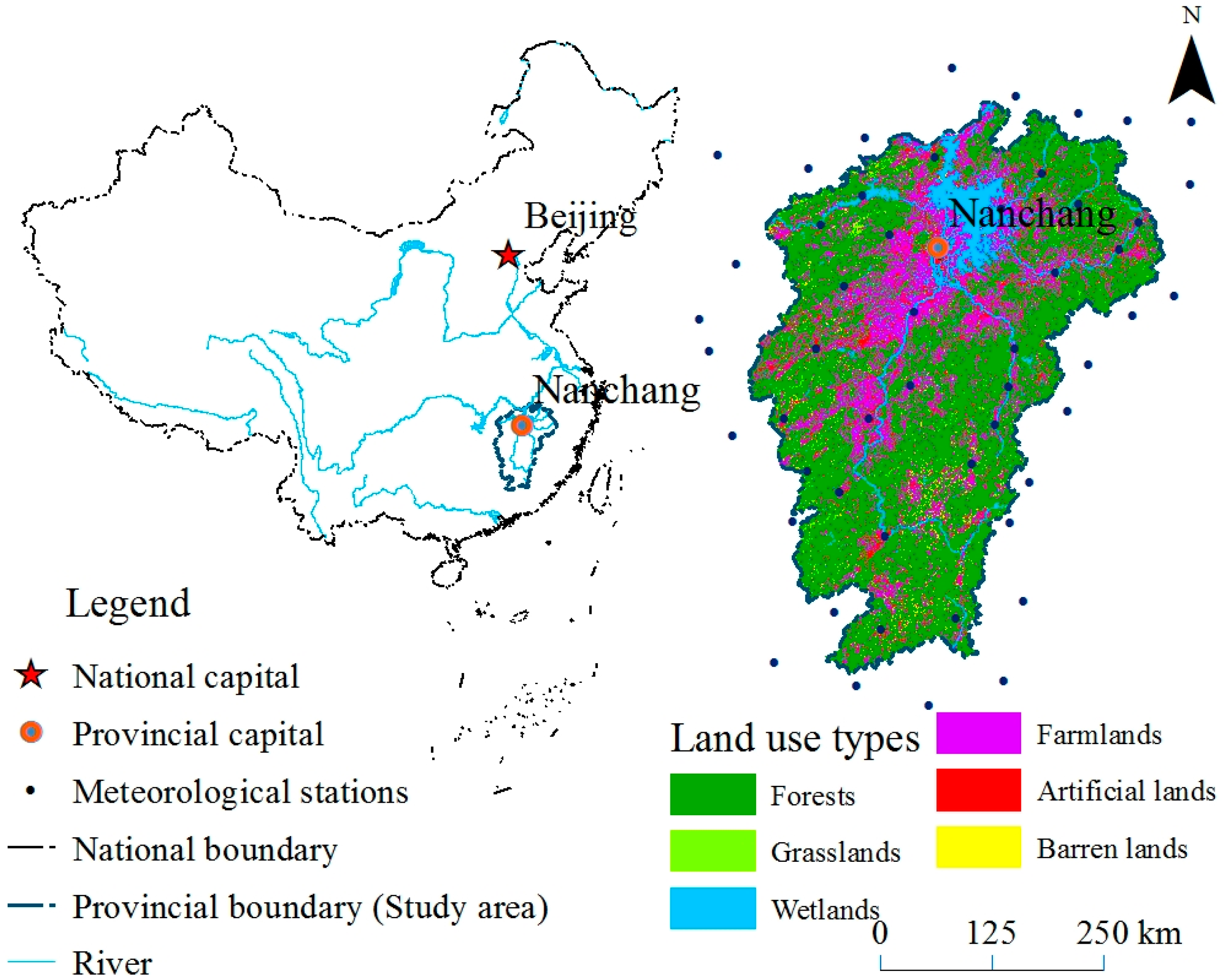
Jiangxi Province (113.57°~118.5°E, 24.5°~30.1°N) is located in the southeastern region of China; the capital is Nanchang (Figure 1). Jiangxi has an area of approximately 167,000 km2 and around 46 million people (Census 2016). The mean altitude of Jiangxi is 249 m, while the maximum and minimum altitudes are 2150 m and 22 m below sea level, respectively. The topography of Jiangxi consists of higher mountain ranges in the southern areas and the marginal areas of the entire province, and small hills and lowlands in the central and northern parts of the province. The province has five large rivers. Gan River, Fu River, Xin River, Rao River, and Xiu River, which flow into Poyang Lake, the largest freshwater lake in China. Poyang Lake is located in the northern part of Jiangxi, which is also home to internationally important freshwater wetlands that serve as habitat for many endangered waterfowl species. Therefore, Jiangxi Province makes up the greatest part of the Poyang Lake basin, approximately 96.6% of whose area is located in the Jiangxi Province [32].
The dominant land use type is forest, which accounts for 66% of Jiangxi’s area, followed by 21% farmland, 6% artificially built-up land, 5% wetland, 2% grassland, and 1% barren land (Figure 1). Major soil types include red soil, weakly developed red soil, and brown soil [33]. The annual mean vegetation coverage of Jiangxi is approximately 65.55%, while the maximum value is 91.97%. The high values of vegetation coverage are mainly located in the mountainous areas, which have a relatively high altitude with relatively low human disturbance. The main climate type in Jiangxi is a subtropical monsoon climate, and the annual mean air temperature and precipitation amount to approximately 18 °C and 1700 mm, respectively. The annual mean air temperature increases from the southwestern to the northeastern region of Jiangxi. The precipitation increases from the northwestern to the southeastern region of Jiangxi [34]. Recently, identifying the hotspots for conserving biodiversity and ESs has been a great concern as population growth and economic development have continued to impose enormous pressures on Jiangxi Province’s natural environment [35] (Figure 1).
2.2. Data Sources
The critical data of the soil conservation mapping methods were obtained as follows. The daily meteorological data (solar radiation, precipitation, and temperature) for the year 2000 and 2010 were retrieved from the China Meteorological Data Service Center [36].The 52 meteorological stations (Figure 1) within and around Jiangxi Province were used to produce the interpolation raster maps (250 m resolution) by using the Kriging method of the ArcGIS 10.2 software. The 250 m MODIS NDVI data were composites of 16-day NDVI maximum values and were acquired from the Level 1 and Atmosphere Archive and Distribution System (LAADS) [37].The land use data were interpreted from Landsat 5 TM of the 2000 and 2010 land cover map with 30-m thematic resolution. The vegetation coverage of the 2000 and 2010 used the dimidiate pixel model, which is a simplified linear spectral unmixing method to calculate the coverage of vegetation [38,39]. Topographical parameters were derived from STRM digital elevation data at a resolution of 90 m [40].The soil property data used in the RUSLE model came from the Chinese soil dataset [41]. All data were interpolated or resampled to a 250-m resolution before being input into the ES models for further analysis.
2.3. Soil Conservation Mapping Methods
2.3.1. RUSLE-Based Model for Mapping Soil Conservation
The annual soil erosion can be calculated by means of the RUSLE empirical model [27] as follows [34]:
where A describes the estimated average soil loss (t·hm−2·year−1); R is the rainfall erosivity factor calculated by means of the Wischmeier empirical formula [27]; Pi identifies the monthly precipitation (mm), and P refers to the annual total precipitation (mm); K is the soil erodibility factor, which was calculated using the EPIC (Erosion—Productivity Impact Calculator) equation [28]; Sa, Si, Cl, and C encompass the percentage (%) of the sand, clay, silt, and organic matter of the soil, respectively; L is the slope length factor [27], and S is the slope steepness factor [42]; m describes a dimensionless constant dependent on the percent slope (); C is the crop and management factor; and P is the conservation practices factor. The values of C and P were the same as in Zhang et al. [34].
If both C and P are assigned a value of 1, then the calculated soil erosion is the potential soil erosion, which presumed the land to be bare or to have no vegetation protection. Therefore, the amount of soil retention can be estimated by the difference between the potential soil erosion and actual soil erosion. The SC model based on the empirical equation of RUSLE is as follows:
where SCRUSLE is the annual amount of soil conserved (t·hm−2·year−1), and the other parameters were calculated in the same fashion as in Equation (1).
2.3.2. The Surrogate Indicator Method for Mapping Soil Conservation Service
The biophysical-based surrogate indicator method for mapping SC can be calculated by Equation (7):
where SCSUR refers to the capability of the SC of the ecosystem, NPP is the sum of the annual net primary production of vegetation, VCnpp describes the standard deviation of the NPP within a year, and K is the soil erodibility factor, which was calculated by means of the EPIC equation (Equation (3)). Fslo refers to the slope of the land surface, which can be calculated using Arcgis10.2 software. The parameters of VCnpp, K, and Fslo were standardized between zero and one by the maximum and minimum value of their values. Lü et al. [30] and Zhang et al. [31], using the modeling framework of this NPP based surrogate indicator, incorporated the K factor into the model, mapped the SC of ecosystems, characterized the spatio-temporal variations of SC in China, and revealed the representation of critical natural capital in China. The above-mentioned works showed the usability and reliability of the NPP based surrogate indicator for mapping SC well.
SCSUR = NPP × (1 − VCnpp) × (1 − K) × (1 − Fslo)
The terrestrial Carnegie Ames-Stanford Approach (CASA) was used to estimate the NPP of vegetation. The CASA model advocates determining the NPP of vegetation as the product of the modulated absorbed photosynthetically active radiation (APAR) and the light use efficiency (ε) factor [43]:
where NPP(x, t) describes the net primary production of location x at time t, APAR refers to the canopy-absorbed incident solar radiation (MJ·m−2), and the parameter is the light use efficiency (g·C·MJ−1). Land cover, NDVI, and climate data are needed for the CASA model. The annual total NPP (g·C·m−2·year−1) is the sum of the NPP during the twelve months within a year [34].
3. Results
3.1. Spatial Patterns of SC
After mapping the SC of Jiangxi Province using the two methods provided in the paper, the spatial patterns of SC were revealed (Figure 2). The results indicated that the spatial patterns of SC maps which using the SCSUR method are heterogeneous and the high SC areas are scattered in regions of high altitude and with a high fractional vegetation cover. The spatial patterns of SC are similar in 2000 and 2010. The high values of SC maps using the SCRUSLE method were located in the southern and northeastern region of the mountain areas of Jiangxi in 2000, and then moved to the middle-eastern and northeastern region of the mountain areas of Jiangxi in 2010. The variation in the spatial patterns using the SCRUSLE method is significantly impacted by the variation in the annual rainfall erosivity factor for Jiangxi. The mean values of SC quantifying by means of the biophysical surrogate indicator (SCSUR) method were 381.43 in 2000, and 385.72 in 2010, while the mean values of SC modeled by the RUSLE-based method are 351.69 t·hm−2·year−1 in 2000, and 579.92 t·hm−2·year−1 in 2010. The minimum values of the results of the two methods are zero, while the maximum values of the two methods increased from the 2000 to 2010.
3.2. SC Variations under Different Land Use Types, Fractional Vegetation Covers and Land Surface Slopes
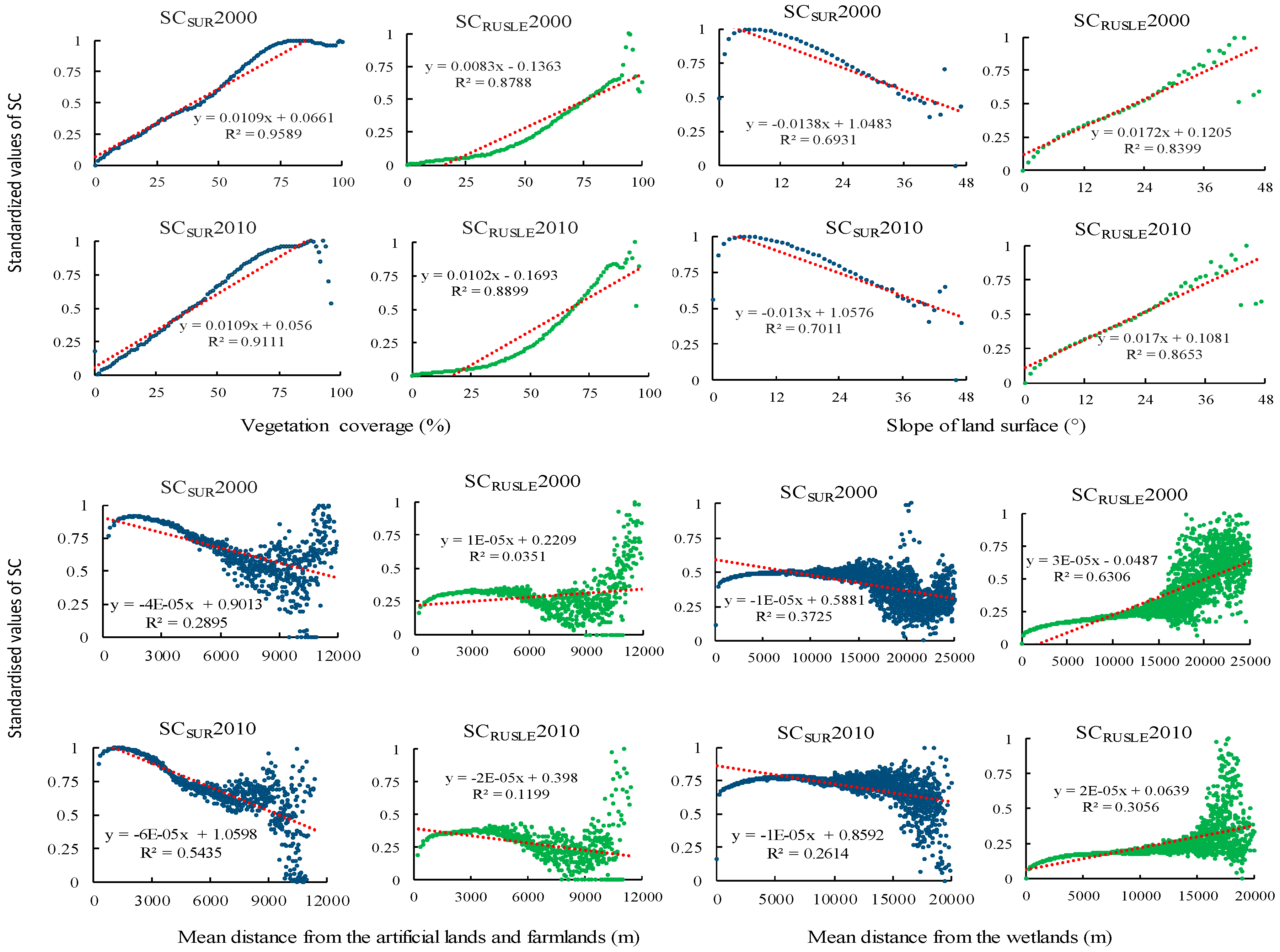
After comparing the differences in the two SC methods in each land use type in 2000 and 2010, the results indicated that variations in the results of the SCSUR model tend to be smaller than the variations of the results of the SCRUSEL model among different land use types (Figure 3). The mean capacities of SC of the SCSUR and SCRUSLE model in each land use type are ranked as follows: forest > grassland > barren land > wetland (Figure 3). The relationship between the results of the two SC methods under different vegetation coverages was analyzed using ArcGIS 10.2 software. The results showed that the values of SC mapped by both the SCSUR and SCRUSLE methods increase with the increase in fractional vegetation covers (Figure 4). The values of SC mapped by the SCRUSLE model increase with the increase in slope; however, the values of SC mapped by the SCSUR method decreases with the increase in land surface slopes (Figure 4).
3.3. Distance Distributions from Artificial Land, Farmland, and Wetland
The spatial patterns of the distance distribution from artificial land, farmland, and wetland of the two SC models were analyzed using ArcGIS 10.2 software, which was based on the raster land use maps for 2000 and 2010. The results showed that the high values of SC mapped by the SCSUR method were located near artificial land and farmland, while the high values of SC mapped by means of the SCRUSLE model were located relatively far from artificial land and farmland. High values of SC mapped by the SCSUR model were located near wetlands, while the high values of SC mapped by the SCRUSLE model were located relatively far from wetlands (Figure 4).
4. Discussion
4.1. Characteristics of Using the Two SC Methods in Practice
The spatial patterns of SC mapped by means of the SCSUR and SCRUSLE methods have certain similarities and differences when used in practice (Table 1). In selecting the appropriate method for mapping SC, decision makers need to consider the different purposes of the task in question, as well as the similarities and differences in the spatial patterns and temporal variations of the priority areas that may arise from using these methods. Because the values of SC of the two mapping methods both increase with increasing of the vegetation coverage, the priority areas for SC selected by the two models will be located in the area in which the fractional vegetation cover is relatively high. Moreover, both mapping methods resulted in higher values of SC in forest and grassland than the other two land use types, which can lead to greater attention given these land uses safeguard the SC capacity of the landscape. Because the values of SC modeled by the SCSUR method decrease with the increasing slope of the land surface while the values of SC modeled by the SCRUSLE method increase with the increase in the slope of the land surface, the priority areas for SC selected by these two methods may differ markedly. Similarly, the priority areas identified by the SCRUSLE model for conserving SC are more likely to be located in precipitous regions than those identified using the SCSUR method.
Given that the distribution of the high values of the SCSUR model are closer to artificial land and farmland than those of the SCRUSLE model, the efficiency of conservation actions in the priority areas of SC identified by the SCSUR model will be higher than that of the SCRUSLE model. In the anthropic zones, disturbance and impacts from human activities on the natural ecosystems were very high; thus, the degradation of the SC was usually more severe in these areas. In contrast, in remote areas, the disturbance of human activities was relatively limited, the cost of building conservation areas to protect the SC will be considerably lower than in nearer anthropic locations. Nevertheless, the SC of the entire region may continue to degrade because the degraded areas of SC are located near anthropic zones, such as croplands and grazing grassland.
Therefore, the two mapping methods have a similar utility in discerning the influence of different land use types and vegetation coverage on the SC, whereas, there are large differences in the representation of the spatial distribution of SC. The slope factor, the rainfall erosivity factor, and the SCRUSLE method as a whole reflect the soil erosion risk [44,45] but not necessarily the ground truth soil conservation capacity of ecosystems. Research based on field observations has revealed important characteristics of the relative ranking stability of different terrestrial ecosystem types on the soil conservation capability in both dry [46,47,48] and humid environments [49]. These ground truth observations under various environmental conditions support the relatively stable pattern of the ecosystems SC (Figure 2A,B) but defy the significant regional spatiotemporal variability of the SC capability (Figure 2C,D). Indeed, the spatial dimension of SC is crucial to land use planning and ecosystem management applications with practical soil erosion and nutrient loss control as key targets. In this sense, SCSUR seems to perform better than SCRUSLE.
4.2. Enlightenment after the Comparison of the Two SC Methods
As humans have already served as an important driving force of various biogeochemical processes on the earth surface, contemporary soil erosion by water can be largely impacted by the interactions between ecosystems and human society under the control of broad environmental regimes (e.g., climate and geomorphology) [50]. Therefore, contemporary soil erosion by water is the final representation of the complex mix from natural erosion and human-accelerated erosion. Humans can never destroy natural erosion or tolerable soil erosion [51]. However, humans’ significant contribution to accelerating and decelerating soil erosion is well documented at various spatiotemporal scales and in various geographical locations [52,53,54,55]. Consequently, one of the key tasks of soil conservation is to avoid human-accelerated erosion [53]. Research also suggests that human-accelerated erosion tends to spread from human disturbance centers to remote areas [56]. The above observations seem to support findings from the SCSUR approach in this research that suggest that the soil conservation service of natural ecosystems is usually higher near anthropogenic land use and wetlands (Figure 4). These may also explain the widespread use of various kinds of vegetated buffer strips to reduce fluxes of eroding soil and associated chemicals from hill slopes into water bodies in mitigating on-site land degradation and off-site water pollution [57,58,59]. However, the conservation values of ecosystems near anthropogenically used lands and wetlands will be largely neglected if solely dependent on the results from the SCRUSLE approach (Figure 4).
The SCRUSLE method can calculate the specific amounts of soil that are conserved in a region, although the accuracy of these amounts of SC cannot be validated because of the absence of suitable observed data on ESs provisioning [60] and the exaggeration of model assumptions, which supposed no vegetation cover in an extremely degraded landscape [21,23,34,61]. In addition, the main limitations of RUSLE-based model are that it requires data at affine spatial scales, the using of this model in the broad spatial scales needs to simplification of the model parameters [62], which may hamper the accuracy and the usability of SCRUSLE in practical applications.
The SCSUR method differs from the SCRUSLE method in that the former is based on the causal relationships between the SC and multiple environmental variables, and the results of the SCSUR method only reveal the relative rankings of the provisioning capability of ecosystems on SC in a region. The SCSUR method incorporates the parameters of NPP into the model, and the NPP is modeled by the remote-sensing data of NDVI and a series of environmental variables. Therefore, the SCSUR method can explicitly relate spatially to the realistic spatial patterns and temporal variations of SC as an important service of ecosystems [16,30,31,63]. These characteristics can meet the needs of policy-making related to soil conservation and ecosystem management, such as the assessment of SC variation caused by changes in land use and the priority setting of conservation planning.
5. Conclusions
Spatially explicit mapping of ESs is the critical method of incorporating ESs into decision-making associated with land use and ecological conservation planning. Traditionally, empirical soil erosion models are usually used to map SC. However, the soundness of these models is largely taken for granted with little verification. Therefore, selecting suitable quantifying methods for SC mapping, especially at a large spatial scale, remains challenging but promising to facilitate conservation decision making and actions. This paper compared a newly formulated biophysical-based surrogate indicator method and a traditional RUSLE based method in SC mapping. Findings suggest that the biophysical indicator method can effectively rank terrestrial ecosystems in terms of their capability to provide SC services at a large spatial scale. The mapping results conform to both findings based on field observations in various environmental settings and the general implementation of soil conservation practices. Therefore, the biophysical indicator method is suitable for large-scale SC mapping meant to support efforts related to soil conservation planning and conservation effectiveness evaluation, despite being much simpler than the traditional empirical models, such as RUSLE. The RUSLE based model is similar to the biophysical indicator method in reflecting different ecosystem (or land cover) types in SC capability ranking. However, the results related to SC spatial patterns are problematic due to lack of support from published literature on soil conservation monitoring and practical applications. This problem may be largely rooted in its very extreme and unrealistic assumption when RUSLE is borrowed to map the SC of ecosystems. In fact, RUSLE has been used and verified globally in soil loss assessment and its environmental risks. However, this support does not necessarily guarantee its usability as a sound SC mapping tool. On the contrary, findings of the present research recommend great caution when using RUSLE to map the SC service of ecosystems, as shown in this paper and the published literature, especially regarding the spatial pattern of SC and its temporal change. Therefore, the newly formulated simple biophysical-based surrogate indicator method is by no means worse at mapping the rankings and spatiotemporal variations of SC in terrestrial environments, and this research revealed the advantages of this new method of SC mapping for soil conservation planning and conservation performance assessment, especially at large spatial scales.
Acknowledgments
This research was funded by the National Key Research and Development Plan of China (2016YFC0501601), the National Natural Science Foundation of China (41601182, 41701478 and 41771220), the Natural Science Basic Research Plan in Shaanxi Province of China (2017JQ4009), and the China Postdoctoral Science Foundation (2016M592743).
Author Contributions
Liwei Zhang analyzed the related data and wrote the manuscript; Yihe Lü designed the framework of the research and revised the manuscript; Bojie Fu gave important advice about the content and writing; and Yuan Zeng provided the land use types and NPP data.
Conflicts of Interest
The authors declare no conflict of interest.
References
- Wilson, K.A.; Underwood, E.C.; Morrison, S.A.; Klausmeyer, K.R.; Murdoch, W.W.; Reyers, B.; Wardell-Johnson, G.; Marquet, P.A.; Rundel, P.W.; McBride, M.F.; et al. Conserving biodiversity efficiently: What to do, where, and when. PLoS Biol. 2007, 5, 12. [Google Scholar] [CrossRef] [PubMed]
- Ferrier, S.; Wintle, B.A. Quantitative approaches to spatial conservation prioritization: Matching the solution to the need. In Spatial Conservation Prioritization: Quantitative Methods & Computational Tools; Moilanen, A., Wilson, K.A., Possingham, H.P., Eds.; Oxford University Press: Oxford, UK, 2009; pp. 1–13. [Google Scholar]
- Lehtomäki, J.; Moilanen, A. Methods and workflow for spatial conservation prioritization using Zonation. Environ. Model. Softw. 2013, 47, 128–137. [Google Scholar] [CrossRef]
- Brooks, T.M.; Mittermeier, R.A.; da Fonseca, G.A.; Gerlach, J.; Hoffmann, M.; Lamoreux, J.F.; Mittermeier, C.G.; Pilgrim, J.D.; Rodrigues, A.S. Global biodiversity conservation priorities. Science 2006, 313, 58–61. [Google Scholar] [CrossRef] [PubMed]
- Paviolo, A.; di Blanco, Y.E.; de Angelo, C.D.; di Bitetti, M.S. Protection affects the abundance and activity patterns of pumas in the Atlantic Forest. J. Mammal. 2009, 90, 926–934. [Google Scholar] [CrossRef]
- Millennium Ecosystem Assessment. Ecosystems and Human Well-Being: Synthesis; World Resources Institute: Washington, DC, USA, 2005. [Google Scholar]
- Egoh, B.; Rouget, M.; Reyers, B.; Knight, A.T.; Cowling, R.M.; van Jaarsveld, A.S.; Welz, A. Integrating ecosystem services into conservation assessments: A review. Ecol. Econ. 2007, 63, 714–721. [Google Scholar] [CrossRef]
- Goldman, R.L.; Tallis, H. A critical analysis of ecosystem services as a tool in conservation projects. Ann. N. Y. Acad. Sci. 2009, 1162, 63–78. [Google Scholar] [CrossRef] [PubMed]
- Polasky, S.; Johnson, K.; Keeler, B.; Kovacs, K.; Nelson, E.; Pennington, D.; Plantinga, A.J.; Withey, J. Are investments to promote biodiversity conservation and ecosystem services aligned? Oxf. Rev. Econ. Policy 2012, 28, 139–163. [Google Scholar] [CrossRef]
- Cowling, R.M.; Egoh, B.; Knight, A.T.; O’Farrell, P.J.; Reyers, B.; Rouget, M.; Roux, D.R.; Welz, A.S. An operational model for mainstreaming ecosystem services for implementation. Proc. Natl. Acad. Sci. USA 2008, 105, 9483–9488. [Google Scholar] [CrossRef] [PubMed]
- Luck, G.W.; Chan, K.M.; Klien, C.J. Identifying spatial priorities for protecting ecosystem services. F1000Research 2012, 1. [Google Scholar] [CrossRef] [PubMed]
- Schulp, C.J.; Alkemade, R. Consequences of Uncertainty in Global-Scale Land Cover Maps for Mapping Ecosystem Functions: An Analysis of Pollination Efficiency. Remote Sens. 2011, 3, 2057–2075. [Google Scholar] [CrossRef] [Green Version]
- Kukkala, A.S.; Moilanen, A. Core concepts of spatial prioritisation in systematic conservation planning. Biol. Rev. 2013, 88, 443–464. [Google Scholar] [CrossRef] [PubMed]
- Daily, G.C.; Matson, P.A. Ecosystem services: From theory to implementation. Proc. Natl. Acad. Sci. USA 2008, 105, 9455–9456. [Google Scholar] [CrossRef] [PubMed]
- Bateman, I.J.; Harwood, A.R.; Mace, G.M.; Watson, R.T.; Abson, D.J.; Andrews, B.; Termansen, M. Bringing ecosystem services into economic decision-making: Land use in the United Kingdom. Science 2013, 341, 45–50. [Google Scholar] [CrossRef] [PubMed]
- Zurlini, G.; Petrosillo, I.; Aretano, R.; Castorini, I.; D’Arpa, S.; De Marco, A.; Pasimeni, M.R.; Semeraro, T.; Zaccarelli, N. Key fundamental aspects for mapping and assessing ecosystem services: Predictability of ecosystem service providers at scales from local to global. Annali di Botanica (Roma) 2014, 4, 53–63. [Google Scholar]
- Xu, W.H.; Xiao, Y.; Zhang, J.J.; Yang, W.; Zhang, L.; Hull, V.; Wang, Z.; Zheng, H.; Liu, J.G.; Polasky, S.; et al. Strengthening protected areas for biodiversity and ecosystem services in china. Proc. Natl. Acad. Sci. USA 2017, 114, 1601. [Google Scholar] [CrossRef] [PubMed]
- De Groot, R.S.; Wilson, M.A.; Boumans, R.M.J. A typology for the classification, description and valuation of ecosystem functions, goods and services. Ecol. Econ. 2002, 41, 393–408. [Google Scholar] [CrossRef]
- Yang, D.; Kanae, S.; Oki, T.; Koike, T.; Musiake, K. Global potential soil erosion with reference to land use and climate changes. Hydrol. Process. 2003, 17, 2913–2928. [Google Scholar] [CrossRef]
- Nelson, E.; Mendoza, G.; Regetz, J.; Polasky, S.; Tallis, H.; Cameron, D.R.; Chan, K.M.A.; Daily, G.C.; Goldstein, J.; Kareiva, P.M.; et al. Modeling multiple ecosystem services, biodiversity conservation, commodity production, and tradeoffs at landscape scales. Front. Ecol. Environ. 2009, 7, 4–11. [Google Scholar] [CrossRef]
- Su, C.H.; Fu, B.J. Evolution of ecosystem services in the Chinese Loess Plateau under climatic and land use changes. Glob. Planet. Chang. 2013, 101, 119–128. [Google Scholar] [CrossRef]
- Guerra, C.A.; Pinto-Correia, T.; Metzger, M.J. Mapping Soil Erosion Prevention Using an Ecosystem Service Modeling Framework for Integrated Land Management and Policy. Ecosystems 2014, 17, 878–889. [Google Scholar] [CrossRef]
- Fu, B.J.; Liu, Y.H.; Lü, Y.H.; He, C.S.; Zeng, Y.; Wu, B.F. Assessing the soil erosion control service of ecosystems change in the Loess Plateau of China. Ecol. Complex 2011, 8, 284–293. [Google Scholar] [CrossRef]
- Andrew, M.E.; Wulder, M.A.; Nelson, T.A.; Coops, N.C. Spatial data, analysis approaches, and information needs for spatial ecosystem service assessments: A review. GIScience Remote Sens. 2015, 52, 344–373. [Google Scholar] [CrossRef]
- Carreño, L.; Frank, F.C.; Viglizzo, E.F. Tradeoffs between economic and ecosystem services in Argentina during 50 years of land-use change. Agric. Ecosyst. Environ. 2012, 154, 68–77. [Google Scholar] [CrossRef]
- Barral, M.P.; Oscar, M.N. Land-use planning based on ecosystem service assessment: A case study in the Southeast Pampas of Argentina. Agric. Ecosyst. Environ. 2012, 154, 34–43. [Google Scholar] [CrossRef]
- Wischmeier, W.H.; Smith, D.D. Predicting rainfall erosion losses: A guide to conservation planning. In Agriculture Handbook No. 537; US Department of Agriculture (USDA): Washington, DC, USA, 1978; pp. 5–8. [Google Scholar]
- Sharpley, A.N.; Williams, J.R. EPIC-erosion/productivity impact calculator: 1. Model documentation. Tech. Bull. U. S. Dep. Agric. 1990, 1, 235. [Google Scholar]
- Sidle, R.C.; Ziegler, A.D.; Negishi, J.N.; Nik, A.R.; Siew, R.; Turkelboom, F. Erosion processes in steep terrain: Truths, myths and uncertainties related to forest management in Southeast Asia. For. Ecol. Manag. 2006, 224, 199–225. [Google Scholar] [CrossRef]
- Lü, Y.H.; Zhang, L.W.; Zeng, Y.; Fu, B.J.; Whitham, C.; Liu, S.G.; Wu, B.F. Representation of critical natural capital in China. Conserv. Biol. 2017, 31, 894–902. [Google Scholar] [CrossRef] [PubMed]
- Zhang, L.W.; Lü, Y.H.; Fu, B.J.; Dong, Z.B.; Zeng, Y.; Wu, B.F. Mapping ecosystem services for China’s ecoregions with a biophysical surrogate approach. Landsc. Urban Plan. 2017, 161, 22–31. [Google Scholar] [CrossRef]
- Yu, J.; Zheng, B.; Liu, Y.; Liu, C. Evaluation of soil loss and transportation load of adsorption N and P in Poyang Lake watershed. Acta Ecol. Sin. 2011, 31, 3980–3989. (In Chinese) [Google Scholar]
- Ding, Q.F.; Wang, J.B.; Qi, S.H.; Ye, H.; Huang, M.; Xu, Y.T.; Ying, T.Y.; Tao, J. Spatial patterns of vegetation net primary productivity in Jiangxi Province of China in relation to climate factors. Chin. J. Ecol. 2013, 32, 726–732. (In Chinese) [Google Scholar]
- Zhang, L.W.; Fu, B.; Fu, B.J.; Lü, Y.H.; Zeng, Y. Balancing multiple ecosystem services in conservation priority setting. Landsc. Ecol. 2015, 30, 535–546. [Google Scholar] [CrossRef]
- He, Y.; Che, T.; Wang, Y. Ecological Footprint and Endogenous Economic Growth in the Poyang Lake Area in China Based on Empirical Analysis of Panel Data Model. J. Resour. Ecol. 2012, 3, 367–372. [Google Scholar]
- China Meteorological Data Service Center, Dataset of Monthly Values of Climate. National Meteorological Information Center, Beijing, China. 2008. Available online: http://data.cma.cn/data/cdcdetail/dataCode/SURF_CLI_CHN_MUL_MON.html/ (accessed on 4 September 2017).
- LAADS. EOSDIS Distributed Active Archive Centers. 2000. Available online: https://earthdata.nasa.gov/about/daacs/daac-laads/ (accessed on 4 September 2017).
- Ivits, E.; Cherlet, M.; Sommer, S.; Mehl, W. Addressing the complexity in nonlinear evolution of vegetation phenological change with time-series of remote sensing images. Ecol. Indic. 2013, 26, 49–60. [Google Scholar] [CrossRef]
- Lü, Y.H.; Zhang, L.W.; Feng, X.M.; Zeng, Y.; Fu, B.J.; Yao, X.L.; Li, J.R.; Wu, B.F. Recent ecological transitions in China: Greening, browning, and influential factors. Sci. Rep. 2015, 5, 8732. [Google Scholar] [CrossRef] [PubMed]
- SRTM 90m Digital Elevation Data. The CGIAR Consortium for Spatial Information. 2003. Available online: http://srtm.csi.cgiar.org/ (accessed on 4 September 2017).
- Chinese soil dataset. China Soil Map Based Harmonized World Soil Database (v1.1). 2009. Available online: http://westdc.westgis.ac.cn/data/611f7d50-b419-4d14-b4dd-4a944b141175/ (accessed on 4 September 2017).
- Zhou, Q.; Liu, X. Digital Topography Analysis; Science Press: Beijing, China, 2006; pp. 79–132. (In Chinese) [Google Scholar]
- Potter, C.S.; Randerson, J.T.; Field, C.B.; Matson, P.A.; Vitousek, P.M.; Mooney, H.S.; Klosster, S.A. Terrestrial ecosystem production: A process model based on global satellite and surface data. Glob. Biogeochem. Cycles 1993, 7, 811–841. [Google Scholar] [CrossRef]
- Delgado, M.E.M.; Canters, F. Modeling the impacts of agroforestry systems on the spatial patterns of soil erosion risk in three catchments of Claveria, the Philippines. Agrofor. Syst. 2012, 85, 411–432. [Google Scholar] [CrossRef]
- Meusburger, K.; Steel, A.; Panagos, P.; Montanarella, L.; Alewell, C. Spatial and temporal variability of rainfall erosivity factor for Switzerland. Hydrol. Earth Syst. Sci. 2012, 16, 167–177. [Google Scholar] [CrossRef] [Green Version]
- Zuazo, V.H.D.; Pleguezuelo, C.R.R. Soil-erosion and runoff prevention by plant covers. A review. Agron. Sustain. Dev. 2008, 28, 65–86. [Google Scholar] [CrossRef]
- Wei, W.; Chen, L.D.; Fu, B.J.; Lü, Y.H.; Gong, J. Responses of water erosion to rainfall extremes and vegetation types in a loess semiarid hilly area, NW China. Hydrol. Process. 2009, 23, 1780–1791. [Google Scholar] [CrossRef]
- Taye, G.; Poesen, J.; Wesemael, B.V.; Vanmaercke, M.; Teka, D.; Deckers, J.; Goosse, T.; Maetens, W.; Nyssen, J.; Hallet, V.; et al. Effects of land use, slope gradient, and soil and water conservation structures on runoff and soil loss in semi-arid Northern Ethiopia. Phys. Geogr. 2013, 34, 236–259. [Google Scholar] [Green Version]
- Huang, Z.G.; Ouyang, Z.Y.; Li, F.R.; Zheng, H.; Wang, X.K. Response of runoff and soil loss to reforestation and rainfall type in red soil region of southern China. J. Environ. Sci. 2010, 22, 1765–1773. [Google Scholar] [CrossRef]
- Lü, Y.H.; Fu, B.J.; Wei, W.; Yu, X.B. Major ecosystems in China: Dynamics and challenges for sustainable management. Environ. Manag. 2011, 48, 13–27. [Google Scholar] [CrossRef] [PubMed]
- Verheijen, F.G.A.; Jones, R.J.A.; Rickson, R.J.; Smith, C.J. Tolerable versus actual soil erosion rates in Europe. Earth Sci. Rev. 2009, 94, 23–38. [Google Scholar] [CrossRef] [Green Version]
- Wei, J.; He, X.B.; Bao, Y.H. Anthropogenic impacts on suspended sediment load in the Upper Yangtze River. Reg. Environ. Chang. 2011, 11, 857–868. [Google Scholar] [CrossRef]
- Maetens, W.; Poesen, J.; Vanmaercke, M. How effective are soil conservation techniques in reducing plot runoff and soil loss in Europe and the Mediterranean? Earth Sci. Rev. 2012, 115, 21–36. [Google Scholar] [CrossRef]
- Bichet, V.; Gauthier, E.; Massa, C.; Perren, B.; Richard, H.; Petit, C.; Mathieu, O. The history and impacts of farming activities in south Greenland: An insight from lake deposits. Polar Rec. 2013, 49, 210–220. [Google Scholar]
- Bhandari, K.P.; Aryal, J.; Darnsawasdi, R. A geospatial approach to assessing soil erosion in a watershed by integrating socio-economic determinants and the RUSLE model. Nat. Hazards 2015, 75, 321–342. [Google Scholar] [CrossRef]
- Haring, V.; Clemens, G.; Sauer, D.; Stahr, K. Human-Induced Soil Fertility Decline in a Mountain Region in Northern Vietnam. Die Erde 2010, 141, 235–255. [Google Scholar]
- Gumiere, S.J.; Bissonnais, Y.L.; Raclot, D.; Cheviron, B. Vegetated filter effects on sedimentological connectivity of agricultural catchments in erosion modelling: A review. Earth Surf. Process. Landf. 2011, 36, 3–19. [Google Scholar] [CrossRef]
- Stutter, M.I.; Chardon, W.J.; Kronvang, B. Riparian buffer strips as a multifunctional management tool in agricultural landscapes: Introduction to the special collection. J. Environ. Qual. 2012, 41, 297–303. [Google Scholar] [CrossRef] [PubMed]
- Gaspar, L.; Navas, A.; Machin, J.; Walling, D.E. Using Pb-210(ex) measurements to quantify soil redistribution along two complex toposequences in Mediterranean agroecosystems, northern Spain. Soil Tillage Res. 2013, 130, 81–90. [Google Scholar] [CrossRef] [Green Version]
- Schulp, C.J.E.; Burkhard, B.; Maes, J.; Van Vliet, J.; Verburg, P.H. Uncertainties in Ecosystem Service Maps: A Comparison on the European Scale. PLoS ONE 2014, 9, e109643. [Google Scholar] [CrossRef] [PubMed] [Green Version]
- Yan, H.M.; Zhan, J.Y.; Liu, B.; Yuan, Y.W. Model Estimation of Water Use Efficiency for Soil Conservation in the Lower Heihe River Basin, Northwest China during 2000–2008. Sustainability 2014, 6, 6250–6266. [Google Scholar] [CrossRef]
- Boardman, J. Soil erosion science: Reflections on the limitations of current approaches. Catena 2006, 68, 73–86. [Google Scholar] [CrossRef]
- Costanza, R.; Fisher, B.; Mulder, K.; Liu, S.; Christopher, T. Biodiversity and ecosystem services: A multi-scale empirical study of the relationship between species richness and net primary production. Ecol. Econ. 2007, 61, 478–491. [Google Scholar] [CrossRef]
Figure 1.
Location, meteorological stations, and land use types in Jiangxi Province, China.

Figure 2.
Spatial patterns of the surrogated soil conservation model (SCSUR) (A,B) and RUSLE-based soil conservation model (SCRUSLE) (C,D) in 2000 and 2010. The results of SCSUR have no units, while the units of the results of SCRUSLE are t·hm−2 year−1.
Figure 2.
Spatial patterns of the surrogated soil conservation model (SCSUR) (A,B) and RUSLE-based soil conservation model (SCRUSLE) (C,D) in 2000 and 2010. The results of SCSUR have no units, while the units of the results of SCRUSLE are t·hm−2 year−1.
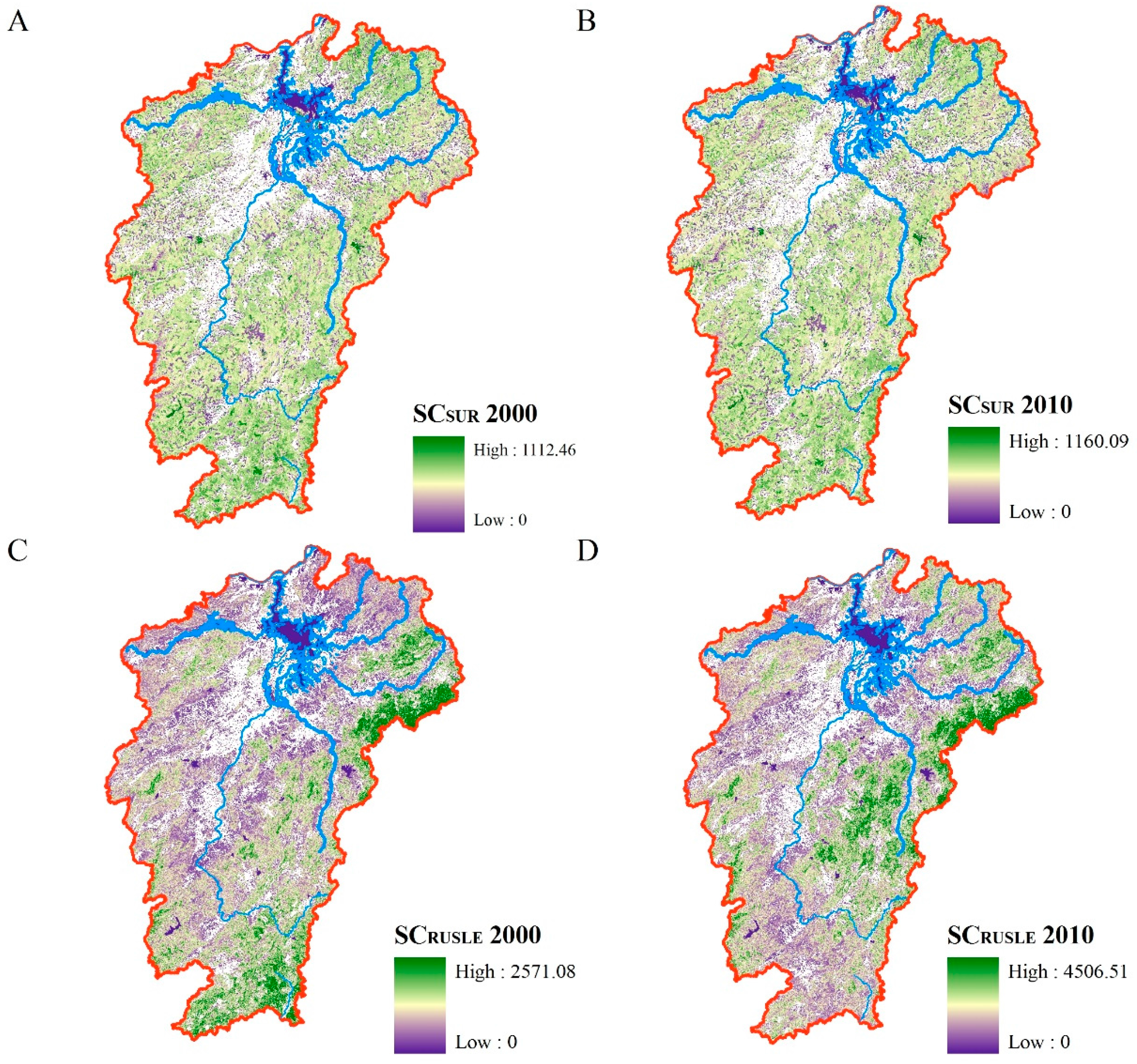
Figure 3.
Variations of the surrogated soil conservation model (SC_SUR) (A) and RUSLE-based soil conservation model (SC_RUSLE) (B) for different land use types in the year 2000 and 2010.
Figure 3.
Variations of the surrogated soil conservation model (SC_SUR) (A) and RUSLE-based soil conservation model (SC_RUSLE) (B) for different land use types in the year 2000 and 2010.
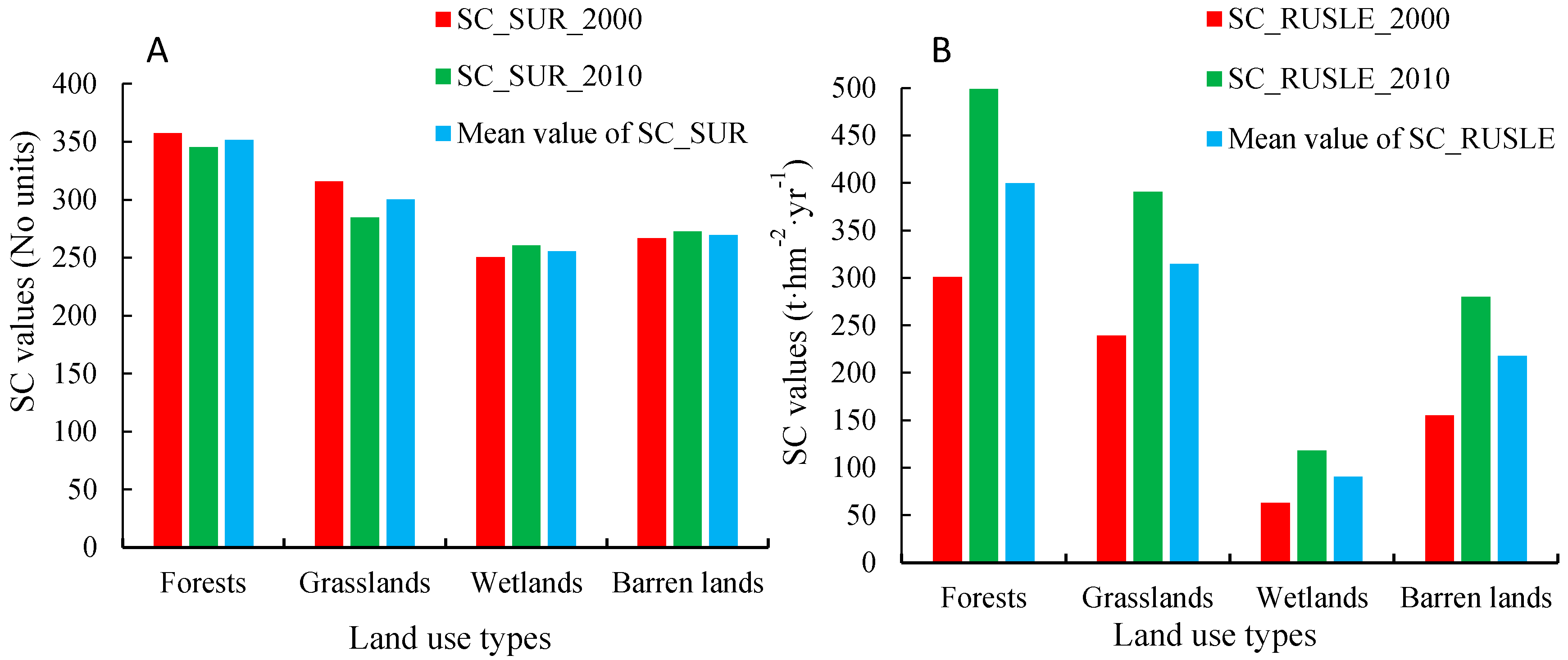
Figure 4.
Variations in soil conservation service (SC) based on different mapping methods under different vegetation coverage and land surface slopes and due to different distances from the artificial lands, farmlands, and wetlands in 2000 and 2010. Both the linear equations are through the significance level of 0.05 of the t-test.


Table 1.
Comparison of the two methods for mapping soil conservation service in the Jiangxi Province.
Table 1.
Comparison of the two methods for mapping soil conservation service in the Jiangxi Province.
| Variables | SCSUR | SCRUSLE |
|---|---|---|
| Land use types | Mean values of the SC of each land use types are: forests > grasslands > barren lands > wetlands | Mean values of the SC of each land use types are: forests > grassland > barren lands > wetlands |
| Slope | Decreases with the increase in land surface slope | Increases with increasing land surface slope |
| Vegetation coverage | Increases with the increasing of the vegetation coverage | Increases with increasing of the vegetation coverage |
| Distance from artificial land and farmland | Close | Far |
| Distance from wetland | Close | Far |
© 2017 by the authors. Licensee MDPI, Basel, Switzerland. This article is an open access article distributed under the terms and conditions of the Creative Commons Attribution (CC BY) license (http://creativecommons.org/licenses/by/4.0/).
Share and Cite
MDPI and ACS Style
Zhang, L.; Lü, Y.; Fu, B.; Zeng, Y. Uncertainties of Two Methods in Selecting Priority Areas for Protecting Soil Conservation Service at Regional Scale. Sustainability 2017, 9, 1577. https://doi.org/10.3390/su9091577
AMA Style
Zhang L, Lü Y, Fu B, Zeng Y. Uncertainties of Two Methods in Selecting Priority Areas for Protecting Soil Conservation Service at Regional Scale. Sustainability. 2017; 9(9):1577. https://doi.org/10.3390/su9091577
Chicago/Turabian StyleZhang, Liwei, Yihe Lü, Bojie Fu, and Yuan Zeng. 2017. "Uncertainties of Two Methods in Selecting Priority Areas for Protecting Soil Conservation Service at Regional Scale" Sustainability 9, no. 9: 1577. https://doi.org/10.3390/su9091577
Note that from the first issue of 2016, this journal uses article numbers instead of page numbers. See further details here.