Effect of Inspection Policies and Residual Value of Collected Used Products: A Mathematical Model and Genetic Algorithm for a Closed-Loop Green Manufacturing System

Abstract

In the green manufacturing system that pursues the reuse of used products, the residual value of collected used products (CUP) hugely affects a variety of managerial decisions to construct profitable and environmental remanufacturing plans. This paper deals with a closed-loop green manufacturing system for companies which perform both manufacturing with raw materials and remanufacturing with collected used products (CUP). The amount of CUP is assumed as a function of buy-back cost while the quality level of CUP, which means the residual value, follows a known distribution. In addition, the remanufacturing cost can differ according to the quality of the CUP. Moreover, nowadays companies are subject to existing environment-related laws such as Extended Producer Responsibility (EPR). Therefore, a company should collect more used products than its obligatory take-back quota or face fines from the government for not meeting its quota. Through the development of mathematical models, two kinds of inspection policies are examined to validate the efficiency of two different operation processes. To find a managerial solution, a genetic algorithm is proposed and tested with numerical examples.

1. Introduction

1.1. Background

Manufacturers are currently seeking continuous growth while minimizing adverse environmental effects from their production activities. They have heavily investigated developing state-of-the-art production technologies that could replace current non eco-friendly production methods. One of the basic approaches is the recycling of used products. Companies try to use reproduced materials as raw materials in their production processes as much as possible if they do not result in negative effects on the quality of the final products. It can not only increase the profit margins of a company but also ensure the prevention of environmental pollution.

There are several reasons that manufacturing companies make significant efforts to protect the environment from their activities. First of all, people do not respect manufacturing companies that emit pollutants during the manufacture process despite producing state-of-the-art products. Companies that do emit high levels of pollutants are increasingly finding that consumers may boycott the company and this can lead to a failure in the market. Secondly, because of the high price of raw materials, recycling itself can be helpful for manufacturing companies. Due to the limit of natural resources, the prices of raw materials tend to increase steadily. Some kinds of packing materials such as plastic bottles, cans, and glass bottles in particular tend to be reused frequently because of the economic benefits. Lastly, some countries have several regulations and governmental policies for the purpose of environmental protection and it forces companies to consider environmentally benign manufacturing in areas such as Europe, Japan, and the USA (as discussed in Allne et al. [1]). Manufacturing companies are limited with regards to the emission of pollutants to prevent air, land, and water pollution. They are also forced to collect used products with an obligatory take-back quota to encourage resource recycling.

There is a regulation called Extended Producer Responsibility (EPR). This regulation gives recycling responsibility to manufacturing companies to encourage recycling and to decrease environmental impacts caused by used products. Therefore, manufacturing companies who produce batteries, tires, or other EPR-applied products or use packing materials such as cans, glass bottles, paper packs, or plastic packing materials should collect used products according to its obligatory take-back quota. If a certain manufacturing company cannot satisfy this responsibility, a heavy penalty greater than the recycling cost of used products will be imposed on that company. Alternatively, manufacturing companies can also entrust responsibility to a third party, called a Producer Responsibility Organization (PRO), and pay relevant costs to the RRO to manage used products. Through the EPR regulation, environmental responsibility of manufacturing companies for several products can be extended to the entire life cycle of them. In Korea, there is a similar regulation to EPR (since 2003) which applies to products mentioned above, and the obligatory take-back quota of each product is set by the government at the beginning of each year; as one example, the obligatory take-back quota of glass bottles was 0.763 in 2015, while in 2014 it was 0.760.

As a result, for the various reasons mentioned above, manufacturers are striving to build recycling and remanufacturing processes that utilize used products. Deng et al. [2] pointed out that one of the most important issues is the residual level of used products and quality management during the remanufacturing process. Therefore, this study investigates the quality decisions on the used product for recycling and remanufacturing process. Furthermore, two quality inspection policies are proposed and compared in terms of various manufacturing factors.

1.2. Problem Description

In this study, we deal with a closed-loop green manufacturing process for a company which performs both manufacturing with raw materials and remanufacturing with collected used products (CUP) to fulfil market demand. The overall manufacturing and remanufacturing process of this company is described in Figure 1.

A company achieves market demand through two sources. First, they purchase raw material and produce new products. Secondly, they produce new products using CUP via remanufacturing. The amount of CUP is assumed as a function of buy-back cost (refer to Equation (1) in Section 3.3) while the quality of used products follows a known distribution. CUP are subjected to quality inspection via policy 1 (model 1) and 2 (model 2). In model 1, inspection is performed for all CUP and products over the minimum quality level of model 1, Q_min,1, are purchased for remanufacturing. In model 2, inspection is performed after buying CUP and products over the minimum quality level of model 2, Q_min,2, are remanufactured. The inspection policy also influences the inspection cost. In model 1, each inspector possesses an inspection device and operates in a specific field. On the other hand, in model 2, the inspection process is performed after buying and collecting purchased products. Therefore, model 2 enjoys economies of scale and it reduces the inspection cost of model 2.

After the inspection process, some of the inspected used products are disposed because of careless handling, etc. In addition, the remanufacturing cost can differ according to the quality of the purchased used products, and the remanufacturing process is performed with used products which have a quality level above Q_min,1 or Q_min,2 for models 1 and 2 respectively. After the remanufacturing process, uncovered customer demand can be satisfied by manufacturing processes using raw materials. In addition, since a company is subject to existing environment-related laws such as EPR, they should ensure they collect a greater amount of used products than its obligatory take-back quota to avoid any potential government fines.

With these circumstances in mind, we examine the efficiency of the two inspection policies, model 1 and model 2. Each inspection policy hugely influences the buy-back cost of used products, quality level, remanufacturing plans, and company profit. Throughout the numerical experiment both policies will be evaluated and compared.

2. Literature Review

Studies on reverse logistics have been investigated since the 1960s. One of the early studies in this field was conducted by Schrady [3]. In this study, the author investigated the deterministic inventory model (EOQ model) for repairable items and suggested a model to determine the optimal procurement and repair quantities. In this model, demand and the return rate were assumed to be deterministic. Infinite manufacturing and the remanufacturing rate were assumed with no disposal. These assumptions were relaxed by the next set of researchers. For example, Mabini et al. [4] extended the model into a multi-product system. Nahmias and Rivera [5] assumed a finite repair rate instead of an infinite rate. Yoo et al. [6] studied pricing and return policies with various supply contracts in a closed-loop supply chain. They assumed that a supplier had more bargaining power than a retailer while the retailer’s decisions on pricing and return policies were influenced by supply contracts. Pricing and remanufacturing decisions in a duopoly market is addressed by Wei and Zhao [7] with two competing supply chains. Through the five game decision models, they suggested equilibrium solutions about the pricing and remanufacturing decisions. Teunter [8] examined an EOQ model of an inventory system with items that can be recovered. In this study, the author considered multiple manufacturing batches including recovery batches. In addition, disposal was allowed. The above studies lie on the deterministic return rate. However, Richter and Dobos [9] and Dobos and Richter [10,11] introduced decision variables on the waste disposal rate and return rate. The optimal collection period for returned products was investigated by Zaarour et al. [12]. The authors considered a closed-loop supply chain with returned products and analyzed discrete and continuous collection periods. Recently, Ma et al. [13] developed closed-loop supply chain models with alliance recycling. Two financing systems were considered, which are pay-as-you-throw and a recycling fund system.

Stochastic models on product quality have also been investigated by several researchers. Salameh and Jaber [14] hypothesized a production/inventory situation where the quality of items is not perfect. Items with imperfect quality could be used in another production chain/inventory. Rahim and Ben-Daya [15] considered joint determination of production quantity, inspection schedules, and quality control for deteriorating products with stochastic product lifetime. A stochastic EOQ model was also suggested. Chang [16] investigated a stochastic inventory model with imperfect quality products which were sold as a single batch at a discounted price. Hwang et al. [17] considered a closed-loop recycling system with the minimum allowed quality level of the returned products. In this study, demand was satisfied by remanufactured products as well as newly manufactured products. Only those used products that satisfy a minimum allowed quality level were bought from the customer for recycling. The authors determine the production cycle and price ratio of returned products relative to a new product and the minimum allowed quality level. Yang et al. [18] introduced an acquisition problem in the presence of uncertain core quality which can influence the production, planning, and control of remanufacturing systems. They derived an optimal solution with expressions in some frequently used quality distributions. Gu and Tagaras [19] examined a reverse supply chain with two independent companies—the collector and the remanufacturer. They tested the optimal collection quantity for the collector and the optimal order quantity for the remanufacturer through the game theory with both deterministic and uncertain demands. Ko et al. [20] conducted cost benefit analysis of standardization of glass bottles. Two competing brewers coordinated their manufacturing operations through standardization. The proposed models determined unit buyback cost for returned products and target inventory level. Recently, Gu et al. [21] proposed a mathematical model for quality design of a non-remanufacturable or a remanufacturable product. In this study, there were options to design a quality of product and the design choices affected both the production costs and consumer valuation associated with the product. Jiang et al. [22] developed an optimal methodology for the selection of remanufacturing process plans. The authors combined the strengths of quality function deployment and fuzzy linear regression to determine the operational decisions in remanufacturing for remanufacturing rates, cost, and quality. More related studies in the field of reverse logistics can be found in Fleischmann et al. [23] and Guide et al. [24]. Also, the impacts and benefits of remanufacturing are investigated in Krill and Thurston [25].

3. Mathematical Model

This section provides notations, assumptions, and the mathematical formulation of the proposed problems. Information about the collection rate and quality distribution of CUPs will be addressed. We consider two inspection policies which are distinguished from the inspection time. In inspection policy 1, the manufacturing company performs an inspection before purchasing, and the inspector only buys used products with a quality level of Q_min,1 or above. In model 2, the manufacturing company purchases used products without inspection, and the inspection process is executed after collection. After the inspection procedure, the remanufacturing process is performed on CUPs with a quality level of Q_min,2 or above. For inspection policy 1, each collector should have suitable inspection skills and spend time inspecting products during collection of used products. On the other hand, for inspection policy 2 inspectors are required in the factory where they perform across the board inspections. As a result, inspection policy 1 requires more expensive inspection costs than that of inspection policy 2. However, there are disposal costs from the disposal of products with a quality level lower than Q_min,2 after inspection for inspection policy 2. As a result, the analysis on the trade-off relationship between the two inspection policies will provide a reasonable collection policy and remanufacturing strategy to maximize total revenue. A typical example of the above policies can be found in the collection of empty bottles and electrical products in Korea.

3.1. Notations

Cins_before	Unit inspection cost before collection
Cins_after	Unit inspection cost after collection
Cmanuf	Unit manufacturing cost
Cdisposal	Unit disposal cost
Craw	Unit raw material cost for manufacturing
Cpenalty	Fine for violating obligatory take-back quota
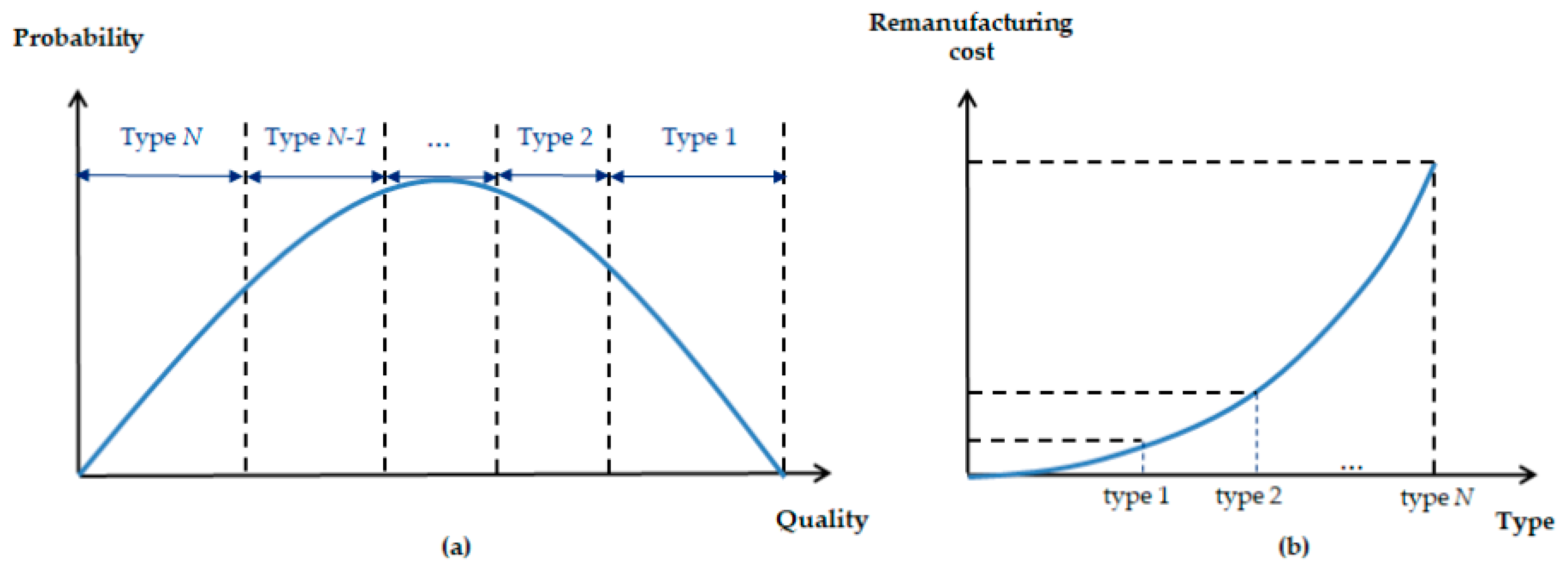
N	Remanufacturing types
Ctype_n	Unit remanufacturing cost for type n, n = 1 ,…, N
Qmin,type_n	Minimum quality level for type n remanufacturing
Q	Quality level of used products, 0 ≤ q ≤ 1
P	Unit sale price for new (or remanufactured) products
πi	Revenue of green manufacturing company of model i
D	Demand for new (or remanufactured) products
R	Amount of CUPs
fc(Cpb)	Collection rate function
fq(x)	Quality distribution of used products
βi	Disposal rate for CUPs for model i
ai, bi	Systemic parameters for disposal rate function for model i
δ	Obligatory take-back quota
dn	An amount of CUP of type n remanufacturing
Qmin,i	Decision variable and minimum quality level of CUPs for model i
Cpb,i	Decision variable and unit buy-back cost for model i

3.2. Assumptions

This section lists assumptions for the proposed problem. Several assumptions about general situations not mentioned here are described in Section 1.2.

A remanufactured product has same product value as a newly manufactured one. It is not an unusual assumption. For example, in the bottle industry, newly manufactured products and remanufactured products have almost identical values in terms of production quality and market value.

It is assumed that the disposal rate of model i for CUPs (β_i) depends on the quality level of the CUP which is a decision variable (Q_min,i) of the proposed study. Equation (1) mathematically shows the relationship between the disposal rate and quality level of the CUP for model i.

$${\beta }_i=a_i\cdot e^{-b_i\cdot Q_{min,i}}fori=1,2$$

(1)

CUPs are divided into maximum N remanufacturing types based on quality and Q_{min,type_n}.

Each remanufacturing type has different remanufacturing costs. As the quality value of used products decreases, the remanufacturing costs increase.

There are no limitations on the supply of newly manufactured products. In detail, manufacturing companies can satisfy demand (D) without remanufactured products.

Figure 2a,b provides graphical descriptions on assumptions 2 and 3.

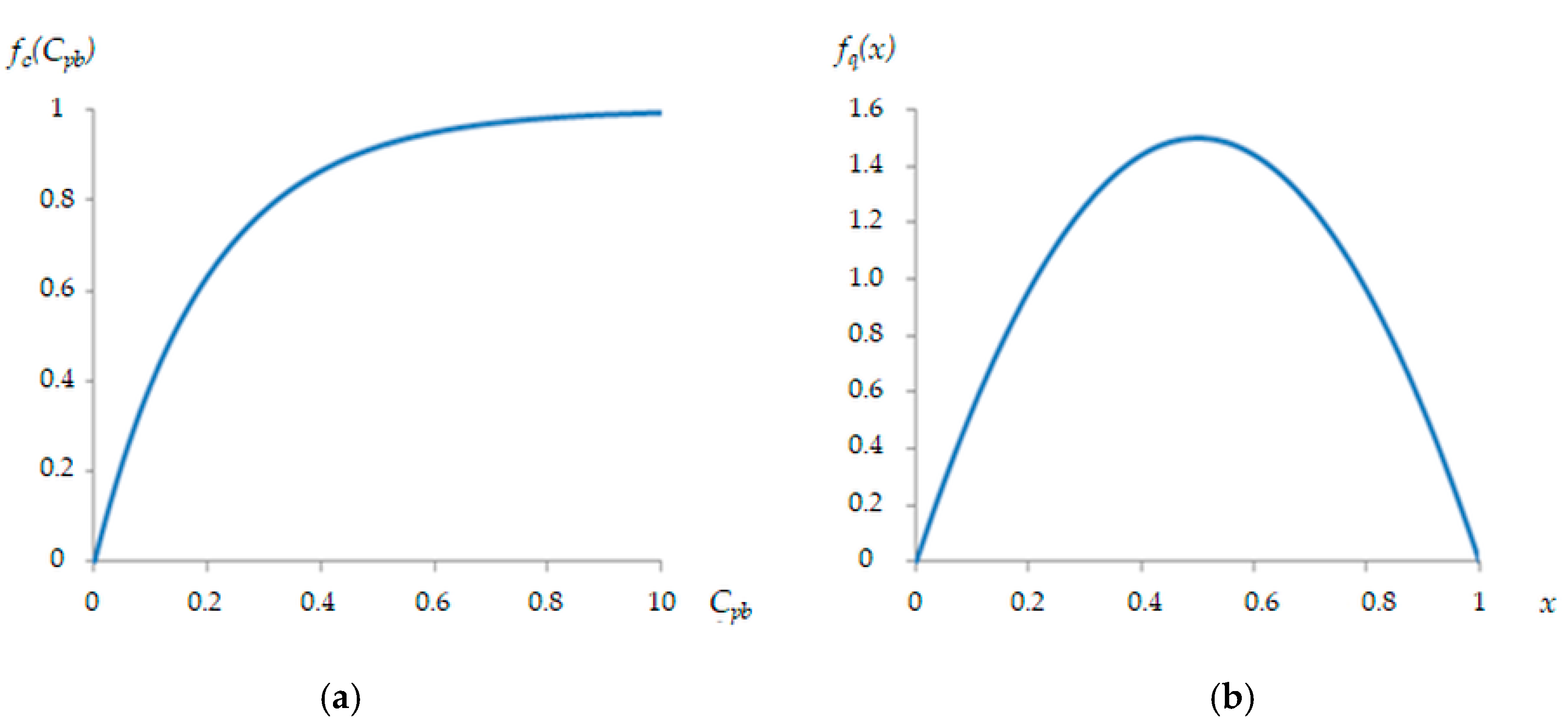
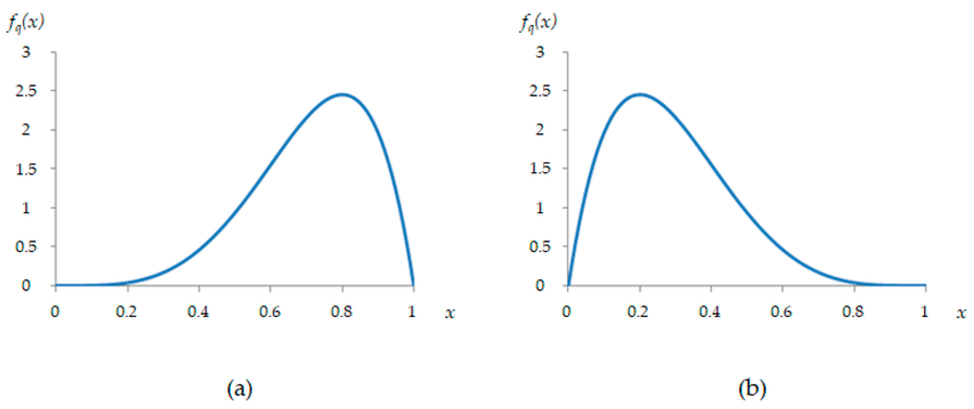
3.3. Collection Rate and Quality Distribuion of Collected Used Products

In this study, it is assumed that the amount of CUPs depends on the buy-back cost. It is assumed to follow the exponential function which is depicted in Equation (2) with a buy-back cost C_p^b. It is a reasonable assumption because the high buy-back cost positively affects the amount of returned CUPs compared to a low buy-back cost. The use of an exponential return rate function on the buy-back cost of returned products can be found in Ko et al. [20] and Ko and Hwang [26].

$$R=D\cdot f_c(C_{pb})=D\cdot \left(1-\frac{1}{e^{C_{pb}/2}}\right)$$

(2)

In addition, the quality of CUPs, f_q(x), is assumed to follow a known distribution. Figure 3 shows the collection rate function which depends on the buy-back cost and quality distribution of used products in the case of beta (2, 2) distribution.

3.4. Objective Functions

3.4.1. Profit Functions of Model 1: Inspection Policy 1

In model 1, the manufacturing company performs an inspection and then purchases CUPs with a quality level of Q_min,1 or above. Equation (3) represents the profit margins of the manufacturing company in model 1.

$$\begin{array}{ll}{\pi }_1=& p\cdot D-\left(C_{raw}+C_{manuf}\right)\cdot (D-{\displaystyle \sum _{n=1}^N{d}_n})-C_{ins\_before}\cdot R-C_{pb,1}\cdot R\cdot {\displaystyle \underset{Q_{min,1}}{\overset{1}{\int }}f(x)dx}\\ & -C_{disposal}\cdot \beta \cdot R\cdot {\displaystyle \underset{Q_{min,1}}{\overset{1}{\int }}f(x)dx}-{\displaystyle \sum _{n=1}^N{C}_{type\_n}\cdot d_n}\\ & -C_{penalty}\cdot Max\{0,\delta \cdot D-R\cdot {\displaystyle \underset{Q_{min,1}}{\overset{1}{\int }}f(x)dx}\}\end{array}$$

(3)

The profit function of model 1 consists of sales profit, manufacturing cost, inspection cost, total buy-back cost, disposal cost, total remanufacturing cost, and fines for not meeting the take-back quota. Please note that because there are several terms in multiplied form with both the return rate, R, which contains the buy-back cost, C_pb,1 and the minimum allowed quality level, Q_min,1, in Equation (3), it is hard to prove its convexity or concavity in a mathematical way.

3.4.2. Profit Functions of Model 2: Inspection Policy 2

In model 2, the manufacturing company purchases CUPs without inspection and after collection the inspection process is executed. After that, the remanufacturing process is performed on CUPs with a quality level of Q_min,2 or above. When the quality level of CUPs is below Q_min,2 they should be disposed of. Equation (4) represents the profit of the manufacturing company in model 2.

$$\begin{array}{ll}{\pi }_2=& p\cdot D-\left(C_{raw}+C_{manuf}\right)\cdot (D-{\displaystyle \sum _{n=1}^N{d}_n})-C_{ins\_after}\cdot R-C_{pb,2}\cdot R\\ & -C_{disposal}\cdot \left\{\beta \cdot R\cdot {\displaystyle \underset{Q_{min,2}}{\overset{1}{\int }}f(x)dx}+R\cdot {\displaystyle \underset{0}{\overset{Q_{min,2}}{\int }}f(x)dx}\right\}\\ & -{\displaystyle \sum _{n=1}^N{C}_{type\_n}\cdot d_n}-C_{penalty}\cdot Max\{0,\delta \cdot D-R\}\end{array}$$

(4)

The profit function of model 2 is similar with that of model 1. However, in model 2, R amount of CUPs are purchased and inspected. In addition, CUPs below Q_min,2 are disposed of.

3.5. Constraints

Model 1 and 2 share constraints. The following equations describe the constraints of the proposed model i = 1 or 2.

$$R=D\cdot f_c(C_{pb,i})$$

(5)

$$d_n=R\cdot \max \left\{0,\left[{\displaystyle {\int }_{q{}_{min,type\_n}}^{q{}_{min,type\_n-1}}{f}_q(x)dx}-\max \{0,{\displaystyle {\int }_{q{}_{min,type\_n}}^{Q_{min,i}}{f}_q(x)dx}\}\right]\right\}$$

(6)

$$0\le Q_{min,i}\le 1$$

(7)

$$C_{pb,i}\ge 0$$

(8)

Equation (5) determines the amount of CUPs. The amount of CUPs of type n remanufacturing is determined via Equation (6). Equations (7) and (8) describe the range of decision variables.

4. Solution Procedure

To obtain a solution for the proposed mathematical formulation we develop a genetic algorithm. The genetic algorithm was first introduced by Holland [27] and currently enjoys wide use as a solution procedure for generating optimal or near-optimal solutions. Examples of its use in manufacturing and remanufacturing fields can be found in Kesen and Güngör [28], Zhang et al. [29], Yildirim and Mouzon [30] and Yan et al. [31]. Also, Liu and Yi [32] developed a genetic algorithm to evaluate the performance of a green supply chain.

The overall procedure of our proposed genetic algorithm is as follows. Let N_c and N_g be the number of chromosomes in a population and number of generations.

STEP 1:	Set generation index i = 0 and current best fitness value = −∞.
STEP 2:	Generate initial population (Nc chromosomes) of ith generation.
STEP 3:	For each chromosome, calculate its fitness value according to Equations (3) and (4) for model 1 and 2, respectively. If the fitness value of a chromosome in ith generation is greater than the current best fitness value, update the current best fitness value and save the corresponding chromosome.
STEP 4:	If i < Ng, create next population for (i + 1)th generation by selection, crossover and mutation in Section 4.3. Otherwise, go to STEP 6
STEP 5:	i← i + 1 and go to STEP 3.
STEP 6:	Finish genetic algorithm.

4.1. Chromosome Structure

In the proposed genetic algorithm, each chromosome represents the value of our decision variables, unit buy-back cost, and minimum quality level. In the numerical example in Section 5, the unit buy-back cost is assumed to vary from $0.00 to $9.99 while the minimum quality level varies from 0.00 to 0.99. Therefore, each chromosome consists of five cells—the first three cells for unit buy-back cost and next 2 cells for minimum quality level. In each cell, an integer value between 0 and 9 is randomly generated. In the initial population, N_c chromosomes are randomly generated.

4.2. Fitness Function

The role of the fitness function in the genetic algorithm is to evaluate the value of each chromosome with respect to the objective function of the mathematical model. As a result, Equations (3) and (4) are used as the fitness function of model 1 and model 2, respectively.

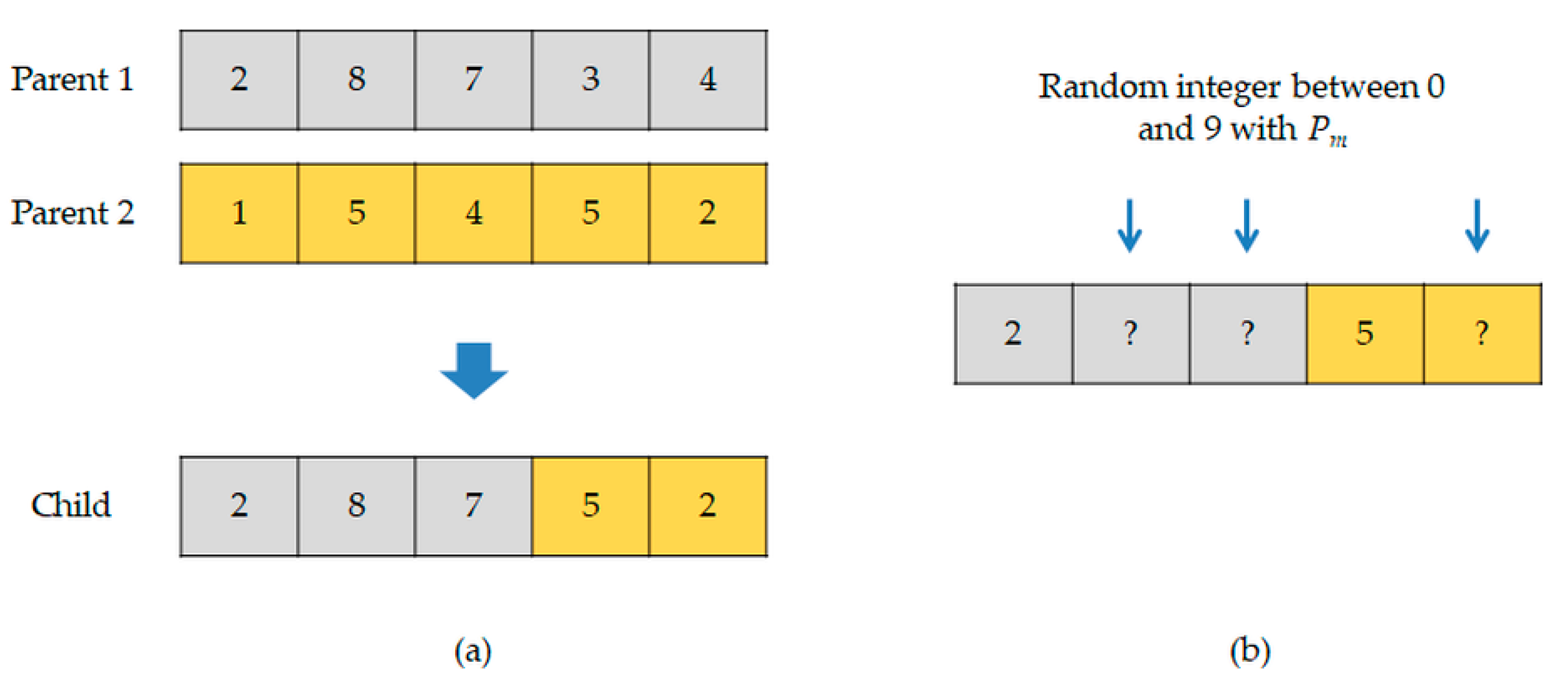
4.3. Selection, Crossover, and Mutation

In the genetic algorithm, the population of the (i + 1)th generation is produced from that of the previous (ith) generation by creating N_c new chromosomes. This process is divided into three parts; selection, crossover, and mutation.

First, two parent chromosomes are selected via the roulette wheel mechanism as follow:

STEP 1:	Let Pi be the population of ith generation. Let Cm be the mth chromosome of population Pi,m∈{1,…, Nc}. Let FF(Cm) be the fitness value of chromosome Cm.
STEP 2:	Calculate
	$$S(C_m)={[FF(C_m)-{\min }_{m\in \{1,...,N_c\}}\{FF(C_m)\}]}^2$$ (9)
STEP 3:	Select chromosome c as Parent 1 with the probability of
	$$S(c)/{\displaystyle {\sum }_{m=1}^{N_c}S(C_m)}$$ (10)
STEP 4:	Repeat STEP 3 to obtain Parent 2

A chromosome with a higher fitness value has more opportunity to be selected via Equations (9) and (10). Selected parents undergo the crossover process with the probability of P_c. In the crossover scheme, one child chromosome is generated from the two parents. The unit buy-back cost of parent 1 and the minimum quality level of parent 2 compose the child node. The generated child then moves to the mutation process. During the mutation, the values of the 2nd, 3rd, and 5th cells are replaced with the probability of P_m by a randomly generated integer in the range of [0, 9]. Each of the N_c chromosomes in the new population is created in the same manner. Figure 4 shows the crossover mechanism (a) and mutation mechanism (b).

5. Numerical Experiments

5.1. Validity Analysis of Proposed Models

5.1.1. Systemic Parameters

Table 1. Data parameters for validity analysis.

Parameter	Value	Parameter	Value
P	$10.00/unit	Ctype_3	1.60
D	10,000 unit	Qmin, type_4	0.60
Cins_before	$0.05/unit	Ctype_4	2.50
Cins_after	$0.03/unit	Qmin, type_5	0.50
Cmanuf	$3.00/unit	Ctype_5	3.50
Cdisposal	$0.10/unit	Qmin, type_6	0.40
Cpenalty	$20.00/unit	Ctype_6	4.60
Craw	$2.00/unit	Qmin, type_7	0.30
(a1, a2, b1, b2)	(0.07, 0.07, 0.03, 0.03)	Ctype_7	5.90
δ	0.70	Qmin, type_8	0.20
Qmin, type_1	0.90	Ctype_8	7.20
Ctype_1	0.30	Qmin, type_9	0.10
Qmin, type_2	0.80	Cype_9	8.60
Ctype_2	0.90	Qmin, type_10	0.00
Qqmin, type_3	0.70	Ctype_10	10.00

shows the data parameters used in validity analysis. CUPs are divided into 10 types (N = 10) based on their quality for the remanufacturing process.

5.1.2. Computational Results

Table 2. Computational results of validity analysis.

	Cpb,i ($)	Qmin,i	Amount of Remanufactured Products Per Type (Unit)										Total Profit ($)	CPU Time (s)
			1	2	3	4	5	6	7	8	9	10
Model 1	2.52	0.09	188	510	752	913	995	995	913	752	510	94	37,230.1	0.235
Model 2	2.41	0.40	192	521	767	932	1014	1014	0	0	0	0	42,810.4	0.192

shows the computational results. For the genetic algorithm, N_c and N_g were both set to 200. The proposed genetic algorithm derives a solution within 0.2 s. In model 1, the company inspects the CUPs and only those with a quality level of 0.09 or above are purchased at $2.52 per each. The total amount of purchased used products are 7000 units (after inspection) to avoid government fines. 378 units are damaged during the collection process or later deemed unsuitable for use, and 6622 units are remanufactured. The company newly manufactures a further 3378 units. In model 2, the manufacturing company purchases 7000 units of CUPs at $2.41 each to avoid government fines. They inspect the CUPs and only remanufacture end-of-products with a quality level of 0.40 or above. Among the 7000 units of purchased used products, 4440 units are remanufactured. 95 units are disposed of and 2465 units are not used. An additional 5560 units of products are newly manufactured.

In the proposed numerical experiment, both model 1 and model 2 decide to purchase 7000 used products for remanufacturing due to the high fine that comes from the violation of ERP. Model 2 achieves greater profits than model 1 due to the lower buying cost and lower inspection cost. Model 2 also focuses on highly valuable used products that have a quality level of 0.40 or above.

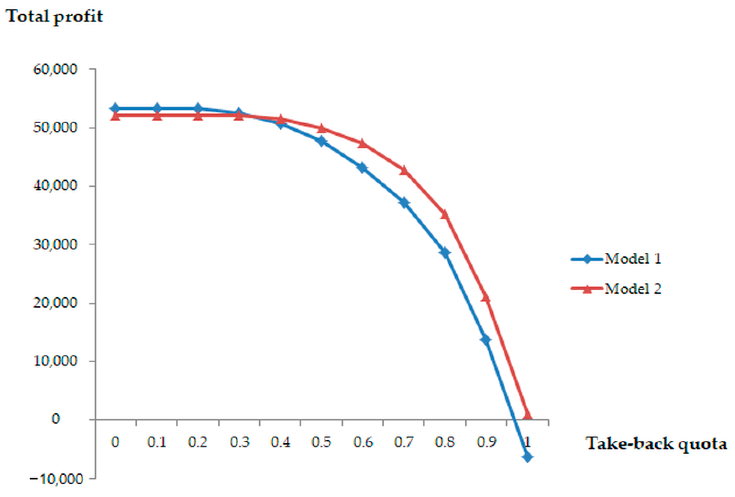
5.2. Sensitivity Test on the Obligatory Take-Back Quota

In this section, model sensitivity on the obligatory take-back quota will be discussed. In the Section 5.1, obligatory take-back quota was set to 0.7. As a result, manufacturing company in each model purchases exactly 7000 used products to avoid the penalty cost. Even in the case of model 2, manufacturing company purchases 7000 units and 2465 units are disused due to the high remanufacturing cost. Obligatory take-back quota was changed from 0.0 to 1.0 and the result was analysed in term of return rate, buy-back cost, minimum quality level and total profit.

Table 3. Results of sensitivity analysis on the take-back quota.

Take-Back Quota		0.0	0.1	0.2	0.3	0.4	0.5	0.6	0.7	0.8	0.9	1.0
Return Rate	M1	0.42	0.42	0.42	0.48	0.59	0.63	0.67	0.72	0.80	0.89	0.89
	M2	0.27	0.27	0.27	0.30	0.40	0.50	0.60	0.70	0.80	0.89	0.89
Buy-Back Cost	M1	1.12	1.12	1.12	1.33	1.79	2.03	2.22	2.58	3.22	4.41	4.41
	M2	0.64	0.64	0.64	0.72	1.03	1.39	1.84	2.41	3.22	4.40	4.40
Min. Quality Level	M1	0.50	0.50	0.50	0.42	0.38	0.30	0.20	0.11	0.01	0.00	0.00
	M2	0.40	0.40	0.40	0.40	0.40	0.40	0.40	0.40	0.40	0.40	0.40

summarizes the results.

The low level of take-back quota does not affect the result. When the take-back quota is less than 0.3, the return rate, buy-back cost, and minimum quality level of both model 1 and 2 do not change. In these cases, the manufacturing company is free from the take-back quota and concentrates on maximizing their total profit. As we mentioned in the introduction, companies collect used products for themselves because of financial benefits regardless of any obligatory take-back quota. However, from the 0.3 level of take-back quota, manufacturing companies increase the buy-back cost and return rate to avoid fines arising from the violation of the take-back quota. When δ is 1.0, the manufacturing company maintains the return rate and buy-back cost, and opts for the government fine instead of purchasing 10,000 units of used products due to the high remanufacturing cost ($10 for type 10).

In model 1, the minimum quality level decreases while the take-back quota increases to avoid ant fines. From the 0.8 level of take-back quota, the manufacturing company purchases used products regardless of the quality level of the used products to avoid fines. However, in the case of model 2, the minimum quality level of used products is fixed at 0.4 for every case. In model 2, the manufacturing company purchases the used products first and conducts inspections later. Therefore, the minimum quality level of used products for remanufacturing does not influence penalties arising from the violation of the take-back quota, and only influences the total profit due to the remanufacturing cost. Note that for the used products of remanufacturing type 7, the remanufacturing cost is $5.90 per unit. In this case, manufacturing new products is more profitable because it only costs $5.00 per unit.

Figure 5 shows the relationship between the take-back quota and total profit. The total profit of both models continuously decreases as the take-back quota increases. For model 1 in particular, the manufacturing company fails to create profits because of the high remanufacturing cost of low quality used products.

5.3. Sensitivity Test on Quality Distribution

In Section 5.1, quality distribution is assumed to follow beta distribution with parameter (2, 2). However, quality distribution of CUPs may differ depending on the type of product. In this section, we will examine two cases which follow beta distribution with parameters (5, 2) and (2, 5). Figure 6 describes the quality distribution of Case 1 with beta distribution (5, 2) and Case 2 with beta distribution (2, 5). Other systemic parameters are the same with those of Table 1.

Table 4. Result comparison of case 1 and 2.

Case1) Beta (5, 2)	Cpb,i ($)	Qmin,i	Amount of Remanufactured Products Per Type (Unit)										Total Profit ($)	CPU Time (s)
			1	2	3	4	5	6	7	8	9	10
Model 1	2.44	0.27	785	1579	1612	1281	849	469	205	29	0	0	52,518.5	0.198
Model 2	2.41	0.40	783	1580	1613	1282	849	436	0	0	0	0	53,202.0	0.190
Case2) Beta (2, 5)	Cpb,i ($)	Qmin,i	Amount of Remanufactured Products Per Type (Unit)										Total Profit ($)	CPU Time (s)
			1	2	3	4	5	6	7	8	9	10
Model 1	2.41	0.00	0	10	60	195	445	806	1217	1531	1500	744	20,865.4	0.191
Model 2	2.41	0.40	0	10	64	206	469	849	0	0	0	0	34,729.7	0.194

summarizes the results of Case 1 and Case 2. In Case 1, the average quality of CUPs is higher than that of Case 2. As a result, the manufacturing company achieves higher profits for both model 1 and model 2 for Case 1. In model 1, the manufacturing company can avoid fines by purchasing used products with a quality level of 0.27 or above. However, in Case 2 the manufacturing company in model 1 should purchase used products regardless of their quality level to avoid fines. In model 2, the manufacturing company buys used products at the price of $2.41 per unit for both Case 1 and Case 2 and uses CUPs with a quality 0.4 or above for remanufacturing. Note that the buy-back cost and minimum quality level of model 2 are the same with those of Section 5.1. However, quality distribution results in huge differences in total profits.

6. Concluding Remarks

In this study, we deal with a closed-loop green manufacturing system for a company which performs both manufacturing with raw materials and remanufacturing with used products where remanufacturing costs differ according to the quality of the CUPs. To evaluate the efficiency of the two inspection policies, inspection before/after purchase, mathematical models containing decision variables of unit buy-back cost and minimum quality level are developed with the objective of maximizing total profit. In addition, an efficient genetic algorithm is proposed as a solution methodology to find an optimal or near-optimal value for these decision variables. To validate the proposed mathematical model and genetic algorithm, numerical experiments are performed with hypothetical system parameters. In both models, the manufacturing company obeys the obligatory take-back quota. In model 1, the manufacturing company actually uses the most CUPs with a high remanufacturing cost. In model 2, the manufacturing company disposes of more CUPs than model 1. On the other hand, model 2 achieved higher profit while complying with the obligatory quota, with lower value products being excluded from the reproduction plan. In addition, we conducted sensitivity tests with the obligatory buy-back cost and the quality distribution of end-of-used products. Through them, we can confirm the effects of the obligatory take-back quota on the return rate, unit buy-back cost, and minimum quality level.

Based on these research results, it is expected that the remanufacturing policy maker can compare inspection policies and derive appropriate managerial guidelines for quality levels and remanufacturing plans. The proposed model can support such decisions by comparing and evaluating company policies and residual values with a variety of managerial data. For further research, a closed-loop green manufacturing system with stochastic situations can be addressed in terms of customer demand and disposal rates. Also, the design of a reverse network with consideration of the residual value of end-of-used products could be another viable research topic.

References

1. Allne, D.; Bauer, D.; Bras, B.; Gutowski, T.; Murphy, C.; Piwonka, T.; Sheng, P.; Suthernald, J.; Thurston, D.; Wolff, E. Environmentally Benign Manufacturing: Trends in Europe, Japan, and the USA. J. Manuf. Sci. Eng. 2002, 124, 908–920. [Google Scholar] [CrossRef]
2. Deng, Q.; Liu, X.; Liao, H. Identifying Critical Factors in the Eco-Efficiency of Remanufacturing Based on the Fuzzy DEMATEL Method. Sustainability 2015, 7, 15527–15547. [Google Scholar] [CrossRef]
3. Schrady, D.A. A Deterministic Inventory Model for Reparable Items. Nav. Res. Log. 1967, 14, 391–398. [Google Scholar] [CrossRef]
4. Mabini, M.C.; Pintelon, L.M.; Gelders, L.F. EOQ Type Formulation for Controlling Repairable Inventories. Int. J. Prod. Econ. 1992, 28, 21–33. [Google Scholar] [CrossRef]
5. Nahmias, S.; Rivera, H. A Deterministic Model for a Repairable Item Inventory System with a Finite Repair Rate. Int. J. Prod. Res. 1979, 17, 215–221. [Google Scholar] [CrossRef]
6. Yoo, S.H.; Kim, D.; Park, M. Pricing and Return Policy under Various Supply Contracts in a Closed-Loop Supply Chain. Int. J. Prod. Res. 2015, 53, 106–126. [Google Scholar] [CrossRef]
7. Wei, J.; Zhao, J. Pricing and Remanufacturing Decisions in Two Competing Supply Chains. Int. J. Prod. Res. 2015, 53, 258–278. [Google Scholar] [CrossRef]
8. Teunter, R.H. Economic Order Quantities for Recoverable Item Inventory System. Nav. Res. Log. 2011, 48, 484–495. [Google Scholar] [CrossRef]
9. Richter, K.; Dobos, I. Analysis of the EOQ Repair and Waste Disposal Model with Integer Setup Numbers. Int. J. Prod. Econ. 1999, 59, 463–467. [Google Scholar] [CrossRef]
10. Dobos, I.; Richter, K. The Integer EOQ Repair and Waste Disposal Model-Further Analysis. Cent. Eur. J. Oper. Res. 2000, 8, 173–194. [Google Scholar]
11. Dobos, I.; Richter, K. A Production/Recycling Model with Stationary Demand and Return Rates. Cent. Eur. J. Oper. Res. 2003, 11, 35–46. [Google Scholar] [CrossRef]
12. Zaarour, N.; Melachrinoudis, E.; Solomon, M.M.; Min, H. The optimal determination of the collection period for returned products in the sustainable supply chain. Int. J. Logist. Res. Appl. 2014, 17, 35–45. [Google Scholar] [CrossRef]
13. Ma, Z.; Hu, S.; Dai, Y.; Ye, Y.S. Pay-as-you-throw versus recycling fund system in closed-loop supply chains with alliance recycling. Int. Trans. Oper. Res. 2016. [Google Scholar] [CrossRef]
14. Salameh, M.K.; Jaber, M.Y. Economic Production Quantity Model for Items with Imperfect Quality. Int. J. Prod. Econ. 2000, 64, 59–64. [Google Scholar] [CrossRef]
15. Rahim, M.A.; Ben-Daya, M. Joint determination of production quantity, inspection schedule, and quality control for an imperfect process with deteriorating products. J. Oper. Res. Soc. 2001, 52, 1370–1378. [Google Scholar] [CrossRef]
16. Chang, H.C. An Application of Fuzzy Sets to EOQ Model with Imperfect Quality Items. Comput. Oper. Res. 2004, 31, 2079–2092. [Google Scholar] [CrossRef]
17. Hwang, H.; Ko, Y.D.; Yoon, S.H.; Ko, C.S. A Closed-Loop Recycling System with Minimum Allowed Quality Level on Returned Products. Int. J. Serv. Oper. Manag. 2008, 5, 758–773. [Google Scholar] [CrossRef]
18. Yang, C.; Wang, J.; Ji, P. Optimal Acquisition Policy in Remanufacturing under General Core Quality Distributions. Int. J. Prod. Res. 2015, 53, 1425–1438. [Google Scholar] [CrossRef]
19. Gu, Q.; Tagaras, G. Optimal Collection and Remanufacturing Decisions in Reverse Supply Chains with Collector’s Imperfect Sorting. Int. J. Prod. Res. 2014, 52, 5155–5170. [Google Scholar] [CrossRef]
20. Ko, Y.D.; Noh, I.J.; Hwang, H. Cost Benefits from Standardization of the Packaging Glass Bottles. Comput. Ind. Eng. 2012, 62, 693–702. [Google Scholar] [CrossRef]
21. Gu, W.; Chhajed, D.; Petruzzi, N.C.; Yalabik, B. Quality Design and Environmental Implications of Green Consumerism in Remanufacturing. Int. J. Prod. Econ. 2015, 162, 55–69. [Google Scholar] [CrossRef] [Green Version]
22. Jiang, Z.; Fan, Z.; Sutherland, J.W.; Zhang, H.; Zhang, X. Development of an Optimal Method for Remanufacturing Process Plan Selection. Int. J. Adv. Manuf. Technol. 2014, 72, 1511–1558. [Google Scholar] [CrossRef]
23. Fleischmann, M.; Bloemhof-Ruwaard, J.M.; Dekker, R.; Van der Laan, E.; van Nunen, J.A.E.E.; Van Wassenhove, L.N. Quantitative Models for Reverse Logistics: A Review. Eur. J. Oper. Res. 1997, 103, 1–17. [Google Scholar] [CrossRef] [Green Version]
24. Guide, D.; Jayraman, V.; Srivastava, R.; Benton, W.C. Supply Chain Management for Recoverable Manufacturing Systems. Interfaces 2000, 30, 125–142. [Google Scholar] [CrossRef]
25. Krill, M.; Thurston, D.L. Remanufacturing: Impacts of Sacrificial Cylinder Liners. J. Manuf. Sci. Eng. 2005, 127, 687–697. [Google Scholar] [CrossRef]
26. Ko, Y.D.; Hwang, H. Efficient Operation Policy in a Closed-loop Tire Manufacturing System with ERP. Ind. Eng. Manag. Syst. 2009, 8, 162–170. [Google Scholar]
27. Holland, J.H. Adaptation in Natural and Artificial System: An Introductory Analysis with Applications to Biology, Control, and Artificial Intelligence; University of Michigan Press: Ann Arbor, MI, USA, 1975. [Google Scholar]
28. Kesen, S.E.; Güngör, Z. Job scheduling in virtual manufacturing cells with lot-streaming strategy: A new mathematical model formulation and a genetic algorithm approach. J. Oper. Res. Soc. 2012, 63, 683–695. [Google Scholar] [CrossRef]
29. Zhang, J.; Liu, X.; Yu, Y.L. A Capacitated Production Planning Problem for Closed-Loop Supply Chain with Remanufacturing. Int. J. Adv. Manuf. Technol. 2011, 54, 757–766. [Google Scholar] [CrossRef]
30. Yildirim, M.B.; Mouzon, G. Single-Machine Sustainable Production Planning to Minimize Total Energy Consumption and Total Completion Time Using a Multi Objective Genetic Algorithm. IEEE Trans. Eng. Manag. 2012, 59, 585–597. [Google Scholar] [CrossRef]
31. Yan, H.S.; Wa, X.Q.; Xiong, F.L. Integrated production planning and scheduling for a mixed batch job-shop based on alternant iterative genetic algorithm. J. Oper. Res. Soc. 2015, 66, 1250–1258. [Google Scholar] [CrossRef]
32. Liu, P.; Yi, S. New algorithm for Evaluating the Green Supply Chain Performance in an Uncertain Environment. Sustainability 2016, 8, 960. [Google Scholar] [CrossRef]
Figure 1. Overall procedure of the proposed manufacturing process.
Sustainability 09 01589 g001
Figure 2. N remanufacturing types (a) and related remanufacturing cost (b).
Sustainability 09 01589 g002
Figure 3. Collection rate function (a) and quality distribution with parameter (2, 2) (b).
Sustainability 09 01589 g003
Figure 4. Example of crossover (a) and mutation (b).
Sustainability 09 01589 g004
Figure 5. Relationship between the take-back quota and total profit.
Sustainability 09 01589 g005
Figure 6. Quality distribution of Case 1 (a) and Case 2 (b).
Sustainability 09 01589 g006