Integrated Proactive Control Model for Energy Efficiency Processes in Facilities Management: Applying Dynamic Exponential Smoothing Optimization

1
College of Management, Xi’an University of Architecture and Technology, Xi’an 710055, China
2
Department of Technology, Illinois State University, Normal, IL 61790-5100, USA
*
Authors to whom correspondence should be addressed.
Sustainability 2017, 9(9), 1597; https://doi.org/10.3390/su9091597
Submission received: 20 July 2017
/
Revised: 10 August 2017
/
Accepted: 4 September 2017
/
Published: 8 September 2017
Abstract
:Sustainable facilities management (SFM) opens the door of opportunity for companies to evaluate the quality of resources and environment management at their facilities. It enables the principles of sustainable development. There is still inefficiency in quantitative research of integrating environmental factors, particularly multi-source data, to monitor and control complicated systems in buildings. The objective of this research is to develop an effective method to dynamically optimize energy efficiency in SFM plans and strategies. The research question is: can the integrated proactive method reduce energy consumption with dynamically adjustable controls? This paper proposes a coordinated proactive control method using dynamic time-series prediction (PCM-DTSP) for SFM, which optimizes system controls by integrating the prediction results and monitored environmental-data. The results show that, after optimization, the temperature fluctuations are reduced to 33.3%. The average temperature and maximum temperature are reduced by 8% and 13.1%, respectively. The instantaneous power consumption was reduced by 0.17 KW per hour for each cooling system unit. The PCM-DTSP method can significantly optimize energy efficiency, which paves the way for long-term comprehensive energy management. The contribution of the research lies in its optimized control of energy consumption, temperature stabilization, and improvement of environmental comfort solutions, which can be generalized to various types of buildings.
1. Introduction
The complexities of building and infrastructure projects are increasing worldwide, which are reflected by the complication of corresponding tools, technologies, and operational controls [1,2]. This creates unprecedented challenges to facilities management (FM) [3,4]. The role of sustainable facilities management (SFM) is critical to the planning, maintenance, and management of these complex facilities [3,5,6]. SFM incorporates the people, place and business with optimized economic, environmental and social benefits of sustainability [7,8]. In addition, SFM requires the integration of multiple disciplines, including mechanical, electrical, plumbing, and fire protection (MEPFP), to ensure the functionality of built environment [5,8]. The practice of SFM upsurges the complexity of MEPFP systems which are critical in facilities management [8].
The management and control of MEPFP systems in a facility are very important in building operation and maintenance of SFM [3,5,9]. Especially in complex projects, such as hospitals, science labs, and technology parks, the total investment of MEPFP systems on average can even reach 50% of the total investment of such a project [3,5,10,11]. The traditional FM on MEPFP systems often needs to follow certain routines [12,13]. The routines are pre-set programs which are static and low in efficiency [13,14]. Therefore, it is of great significance to study dynamic operation and maintenance methods for the management of MEPFP systems to improve system efficiency of SFM. There is an urgent need to extensively investigate adaptive and optimized control models on the Heating, Ventilating, and Air Conditioning (HVAC) systems for SFM [15]. Researchers and engineers consider the energy consumption strategy of static low-temperature settings to be conservative, which causes the cooling systems in buildings to be inefficient [16,17,18,19,20,21,22,23,24,25,26]. This research focuses on the optimization of energy efficiency of the HVAC systems for SFM. The research objectives include the following items: (1) to study the current energy management schemes in HVAC systems; and (2) to develop a proactive control method to stabilize temperatures effectively. In this case, the research question is: can the proactive control method reduce the energy consumption for SFM? The target is to reduce the energy consumption that is wasted in regulating temperature fluctuations.
Currently, researchers, engineers and facility managers notice the urgency of learning and adaptation of different actors at various systems. The understanding of how to control MEPFP systems, together with the administration of facility utilization on various technical, economic, social and geographic scales, has become a precondition for the emergence of sustainable development [27,28]. There are a variety of control schemes developed for thermal management in SFM with the purpose to reduce energy costs [8,29]. For sustainable and smart management of HVAC systems, model-based scheme is able to determine the control strategies and react quickly to the rapid changes of indoor environment [8,29,30]. The Model Predictive Control (MPC) approach is a promising method for analytical control on energy consumption [31]. There are three main MPC methods, including Linear Regression Algorithm (LRA) [29,32], Time Series Prediction Algorithm (TSPA) [29,33], and Artificial Neural Network Algorithm (ANNA) [29,34]. This research suggests integrating TSPA method with multi-source data to develop an optimized on-demand control model for efficient and sustainable energy management. Commercial buildings (e.g., office buildings, classrooms, theaters, and airports) have relatively stable operation schedules. The temperature changes in these buildings follow established patterns typically [12,13,14]. The operation schedule of HVAC systems in a commercial building is usually predictable because the building is mainly for a certain type of business or service. This feature is a necessary condition for the effective application of TSPA in this research.
The system designed in this research is a coordinated proactive control method using dynamic time series prediction (PCM-DTSP) for SFM, which optimizes system controls by integrating the prediction results and monitored environmental data. The aim of the development of this PCM-DTSP system is to optimize energy efficiency, which paves the way for long-term comprehensive energy management. The results of the research demonstrate the optimized control of energy consumption, temperature stabilization, and improvement of environmental comfort. The research method and the PCM-DTSP system can be generalized to SFM of various types of buildings. This research has remarkable contribution to theoretical models and implementation of optimization method in sustainable management of energy use. Compared to static settings, dynamic controls of complex mechanical systems are able to recognize requirements or needs of existing building operation and maintenance and understand the requirements to improve the quality of SFM [35]. The test data of the research show that, after the fulfillment of the optimized method, energy consumption of the samples was reduced. The energy saving would be noteworthy in the operation and management of SFM. The practice helps to improve environmental awareness in policy makers, facility managers, and system engineers.
This paper is organized as follows. In the Introduction Section, the paper discusses the importance of energy management in SFM, explains the research question, and briefly describes the contributions of solving the problem. The Literature Review Section presents different analytical models for energy management and describes how the proposed methodology is different from the state-of-the-art. The Methodology Section discusses the optimized method of cooling systems based on MPC. It includes the integration and optimization subsections. The Result Analysis Section analyzes the actual archived data and compares it with experimental data. The last section concludes this study and elaborates the research limitations.
2. Literature Review
One goal of sustainability in facility management (sustainability facilities management or SFM) is to make sure that all the supporting services offered by FM shall improve the sustainability of the facility customers [5,36]. For buildings, FM and energy management are closely related, because an average 25% of complete operating costs are energy costs [37,38]. The majority of energy consumed in buildings is for the Heating, Ventilating, and Air Conditioning (HVAC), particularly when there are differences between indoor and outdoor temperatures. Energy consumption accounts for about 60% of all delivered energy consumed in buildings [39]. There is an urgent need to extensively investigate adaptive and optimized control models on the HVAC systems for SFM [15]. If buildings are able to respond to energy management schemes through advance operation strategies and smart grid infrastructure, it will help to avoid waste of electricity [38]. Consequently, the proposed strategy focuses on managing HVAC systems, considering commercial buildings.
2.1. Optimization Approaches for System Efficiency in Sustainable Facilities Management
Model based predictive control (MPC) has been used widely in chemical plants, oil refineries and other process industries since the 1980s. Presently, MPC is also used in power systems as balancing models [40]. MPC is important to active operations of HVAC systems [41]. As the basis of MPC, energy forecasting models need to have high fidelity and computationally efficiency in electrical systems of buildings [42]. The energy forecasting models can crucially affect the energy consumptions in HVAC systems [21,43]. To improve energy efficiency, it is critical to optimize system operations in SFM [44]. There are two approaches to address the optimization of HVAC system efficiency in buildings [17,18,20,22,23,25]. The two approaches include optimization of airflow organization and enhancement of AC control. The first approach is to optimize the airflow organization of HVAC systems for the purpose of improving system efficiency. For example, in the research project of Ham et al. [18], the modular building used closed cold/hot channels to arrange airflow. Another example is the natural-air cooling systems introduced by Ogawa et al. [22] to reduce energy consumption. Endo et al. proposed a cooling control method based on the predictions of the thermal management requirements at a modular building [19]. The method directly utilized fresh air to cool down temperatures following calculated predictions. Endo et al. claimed that they were able to achieve a satisfactory balance between the thermal requirements and energy savings. Nonetheless, the system depended excessively on the air temperature of external environment. Overall, the first approach is limited on the energy efficiency of HVAC systems.
The second approach is to enhance the control of heating/cooling systems by reducing redundant heating/cooling supply. For example, Oxley et al. studied the improvement of computer room air conditioners (CRAC) for heterogeneous high-performance systems under thermal and energy constraints [23]. Ogawa et al. [22] and Durand-Estebe et al. [17] suggested to optimize the controls of fan speeds for temperature control. Thota et al. studied how to forecast cooling loads for temperature control [25]. Particularly, Huang et al. recommended to determine the set points of air conditioners based on the utilization level of a building [20]. However, the approach failed to minimize the overall energy consumption of the systems and fans. Zhou et al. studied the improvement of cooling efficiency through localized and optimized cooling resources [26]. Zhou et al. suggested to use adaptive vent tiles mounted on floor and control cooling provisions to reduce costs [26]. However, the suggestion did not consider the power consumption of cooling fans. For dynamic service provision, researchers studied the method of using workload predictions for buildings [45]. For example, Yin and Sinopoli developed the approaches that coordinated service provision with thermal-load awareness in job scheduling [45]. However, the coordinated method simply considered the control strategy in two stages. Stage 1 was to find the optimized capacities at different areas. Stage 1 was to use the capacities as the load balancers to calculate the optimized quality-of-service cost. The coordinated method did not integrate the nonlinear changes of loads. It had very limited consideration on the dynamic features of cooling systems. Table 1 is a comparison of the two approaches. It lists the characteristics of the different optimization methods of control schemes for energy management.
2.2. Algorithms of Model Predictive Control
Currently, designers often implement steady-state algorithms in energy management models to reduce redundant cooling supply in HVAC control systems, indicated as the second approach in the previous discussion [46,47]. The purpose of the applications are to establish job schedules for HVAC control systems with thermal-load awareness capacities [47,48]. Such methods are not applicable under dynamic service provision, especially when the environmental temperatures change frequently and unpredictably.
To gain the dynamic feature in the controls of HVAC systems, MPC uses model-based advanced technology with analytical regulators. At present, the main MPC methods are Linear Regression Algorithm (LRA) [32], Time Series Prediction Algorithm (TSPA) [33], and Artificial Neural Network Algorithm (ANNA) [34]. Zhou et al. analyzed LRA and nonlinear regression energy models based on performance counters and system utilization [32]. They proposed a regression energy model with support vectors. Because the thermal distribution of was a slow process, the selected parameters in the regression model would be too sensitive for thermal management [26]. Tarutani et al. proposed a method to predict the temperatures of sensors and the outlet temperature of an air conditioner by using regression models [33]. The prediction method contained TSPA. The predicted results were used to change the parameter settings of the air conditioner. However, in the research of Tarutani et al., only the latest temperature was considered in the forecast. Moreover, only the maximum temperature prediction was selected in the process [33]. The physical space relationship between air conditioners and sensors was not considered. An example of ANNA can be found in Ahn et al., who proposed a comparative analysis of the controllers of heated air supply [34]. The analysis dealt with the amount of mass and air temperatures by using ANNA. They aimed to control the mass and temperatures of supply air per users’ demands. However, there was a lack of consideration of room temperature distribution in the learning model [34].
The LRA, TSPA and ANNA all have advantages and disadvantages. In a LRA Model, the selections of variables and parameters are very important. The selections of parameters directly affect the accuracy of the prediction model. Nevertheless, many factors affect the thermal distribution. Hence, it is difficult to select the variables or parameters accurately when using LRA. TSPA depends on the continuous development of temperatures, using the statistical analysis of historical temperature data to predict the development trend of current temperature. TSPA uses time series data. When great changes take place in time series data, it affects the prediction results. Thus, TSPA is more suitable for short-term forecasts than long-term ones. ANNA is capable of nonlinear mapping and self-learning. However, the predictive ability of ANNA depends on the maturity of its training model. Because of the slow convergence of the algorithm, it has the problem of lags in dynamic control of air conditioners. When selecting an optimization control method for cooling systems, it is necessary to meet the requirement of rapid optimization control of the cooling systems in short term, following the trend of temperature changes.
3. Methodology
This paper proposes a proactive approach to reduce potential hot spots (i.e., areas with high temperatures) in buildings. Figure 1 shows the research design. The first step is to use a dynamic smoothing coefficient to optimize the exponential smoothing method when predicting the changing temperatures of a building. The second step integrates the prediction results and the temperatures detected by sensors to optimize the proportional-integral-derivative controller (PID controller) of air conditioners. The last step is to implement the modified TSPA as an optimization control method for building cooling systems. The proactive control method is able to stabilize building temperatures more effectively than LRA. With a relatively stable temperature, the cooling system of a building would need less energy compared the one with an ever-changing temperature, which helps reduce the energy consumption of the building. This paper contributes to optimized control of indoor air temperature by implementing a dynamic exponential smoothing algorithm. The model-based predictive control in this research successfully combines dynamic smoothing coefficient with incremental PID control algorithm in the control of the air conditioner.
3.1. Predicting Temperature Changes: Forecasting Model Using Exponential Smoothing Method
Exponential smoothing method (ESM) is an experimental technique for time series analysis and prediction (TSPA) [49]. The ESM used in this research is to forecast the temperature at moment based on collected temperature data. This research uses triple exponential smoothing algorithm to precisely catch the trend of temperature changes [49,50]. The following sections discuss single, double and triple exponential smoothing algorithms.
3.1.1. Single ESM Algorithm and Temperature Prediction
Equation (1) shows the single or first-order exponential smoothing (ESM) algorithm, which is the simplest scheme in ESM. It is suitable for the prediction of time series without trend patterns. The result of Equation (1) is a single exponential smoothing (SES) value. The function displays data in a horizontal pattern. Its use is limited to time series data with stationary characteristics.
is the forecast temperature value of time period t. is the collected temperature time series from real-world buildings. is a smoothing coefficient, . The superscript means the first order in exponential smoothing algorithm. is the exponential smoothing value of period . When , the initial value of is the average of the latest 3 temperature values observed before the period 0. is the instantaneous temperature value at period , which refers to the time interval of temperature collection. Usually the time interval is 5 min [49,50]. Based on Equation (1), Equation (2) shows the temperature prediction. The exponential smoothing value is used as the prediction value for t + 1 period.
3.1.2. Double ESM Algorithm and Temperature Prediction
Double ESM calculates the trend pattern of temperatures. It is suitable for the prediction of linear time series. Equation (3) calculates the forecast temperature value of at time t using double ESM.
where is the value of single ESM calculated in Equation (1). Indoor temperature changes frequently and in non-linear patterns. Because of this characteristic, double ESM can be used to predict temperature in a relatively short time period. When the temperature time series with a straight line trend, similar to the trend of moving average method, can be represented by a linear trend model as Equation (4),
where are calculated as follows [49]:
3.1.3. Triple ESM Algorithm and Temperature Prediction
Equation (5) shows the function of triple ESM.
In essence, triple ESM is a quadratic polynomial exponential smoothing function [51]. It is transformed from a linear exponential smoothing method to a non-linear quadratic polynomial exponential smoothing method [34]. It is ideal for describing the characteristics of nonlinear changes of loads and temperatures. Using the same transformation process as for Equation (4), Equation (5) can be rewritten as Equation (6).
where is the prediction period, ;
In Equations (1), (3) and (5), the smoothing coefficient reflects the influence of the measured data on the predicted values. The greater is the value of , the larger is the effect. Meanwhile, the smaller is the deviation between the measured value and the predicted value, the higher is the accuracy of the prediction. Therefore, it is possible to obtain by calculating the squared sum of the deviations of multiple predicted values [51]. Equation (7) shows the formula for calculating the sum of squared deviations.
where is the count of predicted temperatures; represents the temperature predicted at the moment of ; and is the measured temperature at the moment of t.
3.2. Dynamic Exponential Smoothing Optimization Algorithm
Usually, the smoothing coefficient of an ESM for forecasting is a static parameter based on experience [51]. However, the temperatures in a building usually have changes. It is difficult to adapt to temperature changes with empirical measured values and static parameters only. Based on practical experience, if a time series has obvious tendency to change, the smoothing coefficient should take a large value [51]. According to empirical studies and lab experiments [52], usually the value range is . If the time series changes slowly, the smoothing coefficient would be a small value with the range of . If the time series has irregular fluctuations and the long-term trend is approximately a stable constant, the smoothing coefficient is generally very small with the value range of . To precisely predict dynamic temperature changes, this paper uses the correlation analysis to determine the smoothness of time series data and dynamically selects smoothing coefficient parameters, to optimize the temperature prediction method of exponential smoothing.
Each element in the series is a random variable. Its expectation can be expressed as Equation (8):
Equation (9) calculates the variance to measure the discrepancy of the time series between collected data and predicted values:
Equation (10) defines the covariance between the two time series and of the -th period:
Therefore, Equation (11) defines the correlation function of time series:
Equation (12) calculates the variance of a stationary time series when it is a constant:
Thus , when , .
The following steps show the determination method of the smoothness of a time series using the correlation function.
- For the values in the time series starting at a point of time , calculate the correlation coefficient of , where , and is the size of the series . The constant parameter M is the modified length of the time series for correlation calculation. It is used to define the length of the time series. The calculation of M is based on empirical experiments or observations [49,52].
- Calculate the percentages of , in the number of M.
- Depending on whether the percentage of falls within the confidence interval and distribution in the region , determine the stability of temperature time series.
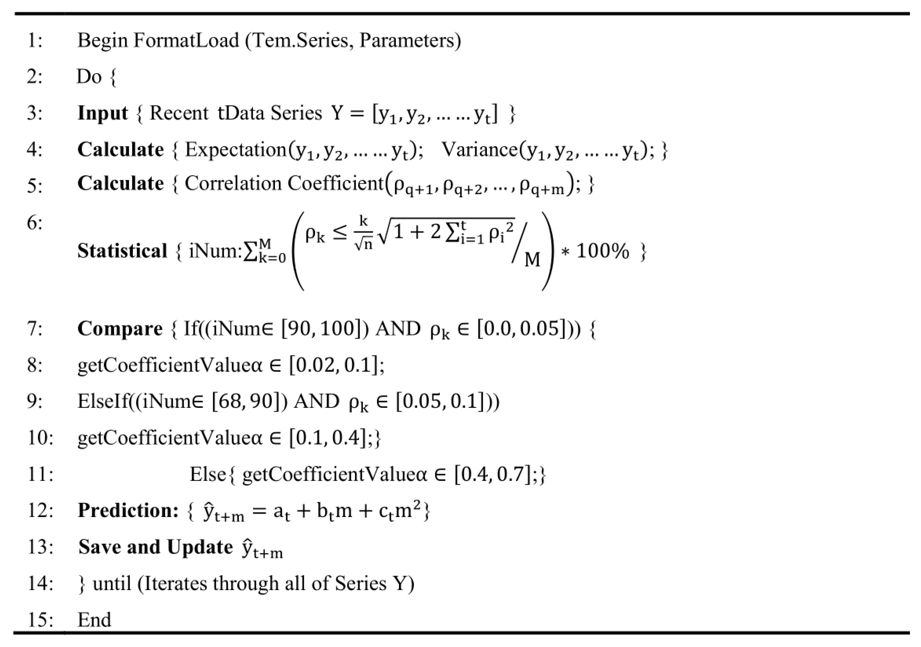
Figure 2 shows the pseudo code of prediction process using the dynamic ESM as the forecasting algorithm (or Dynamic Time-Series Prediction, DTSP). For the purpose of statistical analysis, the maximum value of n is set as 100, which will provide enough sample size for T-test. In Figure 2, are used to calculate the dynamic values of . Once the value of is obtained, the DTSP algorithm will calculate temperature predictions using Equations (5) and (6) accordingly.
In Figure 2, the function of “getCoefficientValue” is based on the minimum target of Squared Sum Error (SSE) expressed in Equation (7). It is rewritten in Equation (13):
where is the collection value in the time series ; and is the temperature prediction value based on triple ESM. This research uses steepest descent method to solve the nonlinear optimization model and sets as the end control condition [53,54,55,56]. Since the precision of the temperature sensors used in the experiment is 0.5 °C, the end control condition is set as . This research takes based on empirical observation [53,54,55,56]. The calculation process is as follows:
- Traverse each smoothing coefficient within a specific range , to calculate the . When a value of makes , the value is selected and the iteration calculation stops.
- If for all the in the range, the algorithm finds a smoothing coefficient which minimizes the in the range. The corresponding is used as the target value.
3.3. System Verification: Prediction Model Using Multi-Source Data
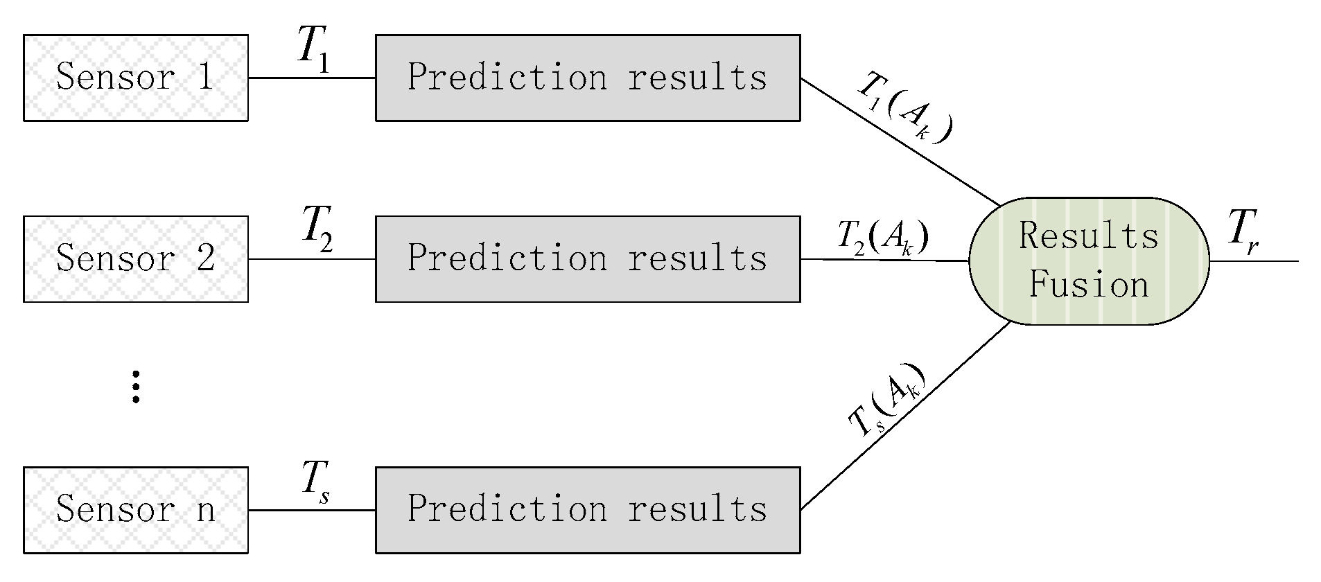
Let represent the sensor in the effective control of the air conditioner . is the real-time temperature acquisition value of sensor . Using the triple ESM algorithm to predicate the indication on the sensor , is the temperature prediction result of sensor in the jth acquisition cycle. The time span of the predicted value determines the weights of the predicted value at different cycles. , and . The superposition of the prediction results of j-th cycle indicates the prediction for each sensor. Equation (14) shows how to calculate the prediction result using the temperatures of multiple acquisition cycles for each sensor.
When predicting temperature, it is necessary to incorporate the prediction results of multiple sensors and select different weights for each sensor. In this study, according to the physical space relationship between air conditioners and sensors, different sensors would have different weights of . The shorter the direct distance between a sensor and an air conditioner, the larger the weight value. The sensor which has the longest distance has the weight value of 1. After the integration of the predicted results of all the sensors, Equation (15) obtains the prediction results of the room temperatures. Figure 3 shows the integration process of temperature predictions. Particularly, the temperature time series is regarded as stationary under the following conditions [49,52]: (1) when and the correlation function is in the confidence interval; or (2) when , . Otherwise, the temperature time series is regarded as not stationary. The conditions are empirical observations. In this paper, we use correlation analysis to determine whether the time series of temperature data is stable.
3.4. Proactive Control Method
If people only depend on the sensors of cooling systems to adjust the PID control of a building, its temperature distribution will be unbalanced. Unbalanced temperature distribution is one of the main reasons causing server downtime, especially when the temperature at a hotspot exceeds a certain limit. Figure 4 shows the principle of optimized control based on cooling predictions of the integrated predictive model (IPM). In Figure 4, the load devices and the cooling devices are associated according to their proximities in the physical space. The predicted temperature of the group of cooling devices and the associated sensors would help the IPM to decide on and carry out the dynamic control on the cooling systems. As shown in Figure 4, when , the prediction results of temperatures will be linked to the cooling control logic. The following definitions are for the variables in Figure 4.
is the integration result of temperature predictions.
is the temperature value monitored by the sensors on air conditioners.
is the difference between the temperature setting and the actual temperature .
is the degree of influence of the air conditioner sensors on the PID calculation when performing PID control calculations. , .
When , the cooling control temperature is:; otherwise, . The PID control of the cooling system depends on the temperature prediction by the IPM. It combines the given value with ratio , integral , and derivative of the actual output value . It also generates control volume through linear combination. Equation (16) shows the differential equation of the cooling PID regulator.
where Thus, Equation (17) calculates the incremental PID algorithm based on temperature control:
where , , and . To improve the accuracy of PID control on cooling systems, the input filter of the cooling control value is the deviation . It is not applied directly to the current time when calculating the differential. Instead, is the average of cooling deviations of the samples in the past four cycles. Hence, the cooling control differentials are formed by weighted summation. Equations (18) and (19) are for the optimization of cooling control differential.
4. Experiment Design
To validate the PCM-DTSP system, this research selects a data center building as the experimental data source. This is a small building located in in Shaanxi Province, China. The PCM-DTSP is implemented in the experiment building to optimize the on-demand cooling supplies and acquire actual data of the systems. The data observed on the systems are used to verify that the PCM-DTSP system is able to achieve optimized control. The research also includes random generated data to validate the temperature prediction, analyze the effectiveness of the system for temperature simulation, and statistical testing. The sampling interval is 5 min. There are 100 observations in the experiment. There are three steps in the experimental analysis.
- Use MATLAB 2014a simulation software (MathWorks, Natick, MA, USA) to analyze the effectiveness of temperature prediction algorithm.
- Analyze the effectiveness of the PCM-DTSP system for temperature simulation.
- Implement the controller program for air conditioners and use the optimized controller to test, analyze, and verify the results.
The building has 11 servers and two industrial-type air conditioning (AC) cabinets. The layout of the data center building is shown in Figure 5. The total cooling capacity (the capacity of cooling output of AC units) is 20 KW. Each AC unit has the rated power (the power consumption of an AC unit in the maximum load state) of 3.56 KW. In addition, there are one power distribution cabinet, six temperature sensors, one smart meter, and three Power Distribution Units (PDUs). The energy efficiency of an AC unit can be calculated using the above two measures by: . The total load of a building includes the power of AC units, servers, power distribution equipment, etc. The total load of the experiment building is approximately 10.5 KW. Each unit of cooling equipment provides cold air to different server groups. The integrated prediction model in this research combines the predictions of the temperature sensors in the same server group and controls the cooling systems based on the calculated optimization results for energy consumption efficiency.
5. Result Analysis
5.1. Analysis of Temperature Prediction Algorithm
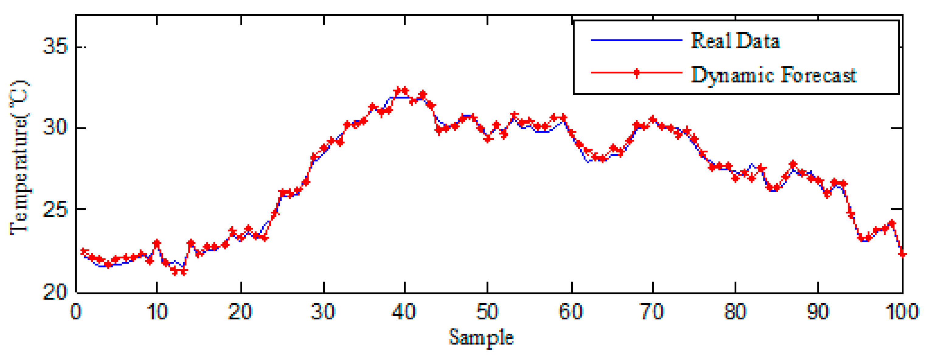
In the experiment of temperature prediction analysis, we used the static exponential smoothing method and the dynamic exponential smoothing method to predict and analyze temperatures. We first used the static smoothing coefficient to predict the temperature trend of the center. In the initial characteristics analysis of the time series curves, we found that the experimental data had relatively slow speed of changes in the whole data sequence. However, there were rapid and frequent changes in local tendencies. Therefore, we selected the smoothing coefficient in the range of [0.1, 0.4]. Appendix A has further explanation of how to choose the value of the smoothing coefficient. However, the static triple exponential smoothing predictive method cannot achieve enough accuracy of prediction. To verify the effectiveness of the proposed algorithm, we used the same set of test data. Figure 6 is the result of using the dynamic smoothing coefficient to predict the building temperatures. It shows that the whole prediction results are in agreement with the actual data. Moreover, the trend of the temperature changes in the building is predicted synchronously as well.
In the process of prediction, the dynamic smoothing coefficient is selected according to the discussion in the Methodology section. The calculation of the range of smoothing coefficient is to validate the selection of the dynamic exponential smoothness, as shown in Figure 6. Figure 7 shows the dynamic changes of the smoothing coefficient. The figure indicates that, to choose the smoothing coefficient , the range should be . Due to the fluctuations of the temperatures in the time series, it is difficult to adapt the whole time series with one single static smoothing coefficient. Its prediction accuracy would be greatly different from the actual monitoring results. The results of the dynamic exponential smoothing method are in good agreement with the actual data samples. The prediction results are better than the static exponential smoothing method. Therefore, it is feasible to predict temperatures by using the dynamic smoothing coefficient in the forecasting model.
5.2. Integration of Predicted and Sensed Temperatures
In the experiment, according to the physical deployment distribution of the equipment and air conditioners, the air conditioners are grouped with the servers and sensors. Figure 5 shows the layout of the groups. In the group binding, some sensors can be shared by the two air-conditioning units at the same time. Hence, they can be used as the basis of analysis for the two groups. The grouping information of the experiment is shown in Table 2.
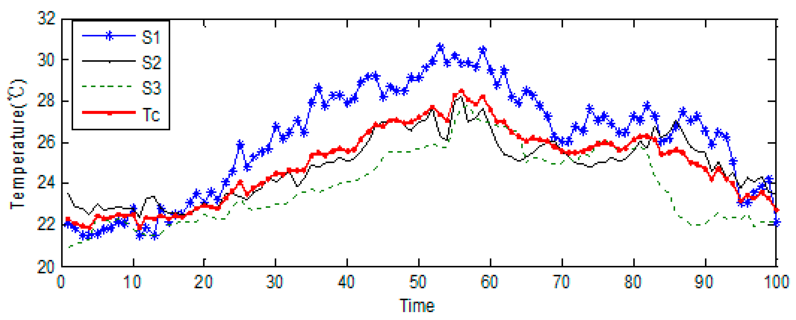
The analysis processes on Groups and are the same. Group is used as experimental object for optimized control analysis. Sensors provide the data series. The temperature difference rate , , and . Based on the grouping information in Table 2, Equations (10) and (11), the process method (Figure 2) of the PCM-DTSP model, and the multi-source data, we selected part of temperature prediction data in Group for integration analysis. Table 3 shows the analysis process and results. Using the analysis results, we obtained the temperature prediction of each sensor in “Group A1”, and the integrated temperature prediction results of “Group A1”. The prediction results of “Group A1” provide the foundation for the integration of multiple sensors. Figure 8 shows the integration results of temperature data from multiple sensors. According to the relationship between and temperature difference rate as shown in Figure 4, the PCM-DTSP model determines whether is involved in air conditioning coordination control. If participates in collaborative control of cooling systems, the temperature control of the air conditioner is ; otherwise the system uses to control the air conditioner. In Figure 8, the curve is an integrated result calculated based on the weight information of the Sensors , and the workflow in Figure 4.
5.3. Statistical Analysis of Cooling Optimization Based on MPC
To optimize the controller of a cooling system, the selection of the PID control algorithm and the adjustment of the parameters can directly affect the result of temperature control of the building. According to the characteristics of the temperature changes, we used the incremental PID control algorithm in the control of the air conditioner of the selected building. The PID parameters of the controller are shown in Table 4.
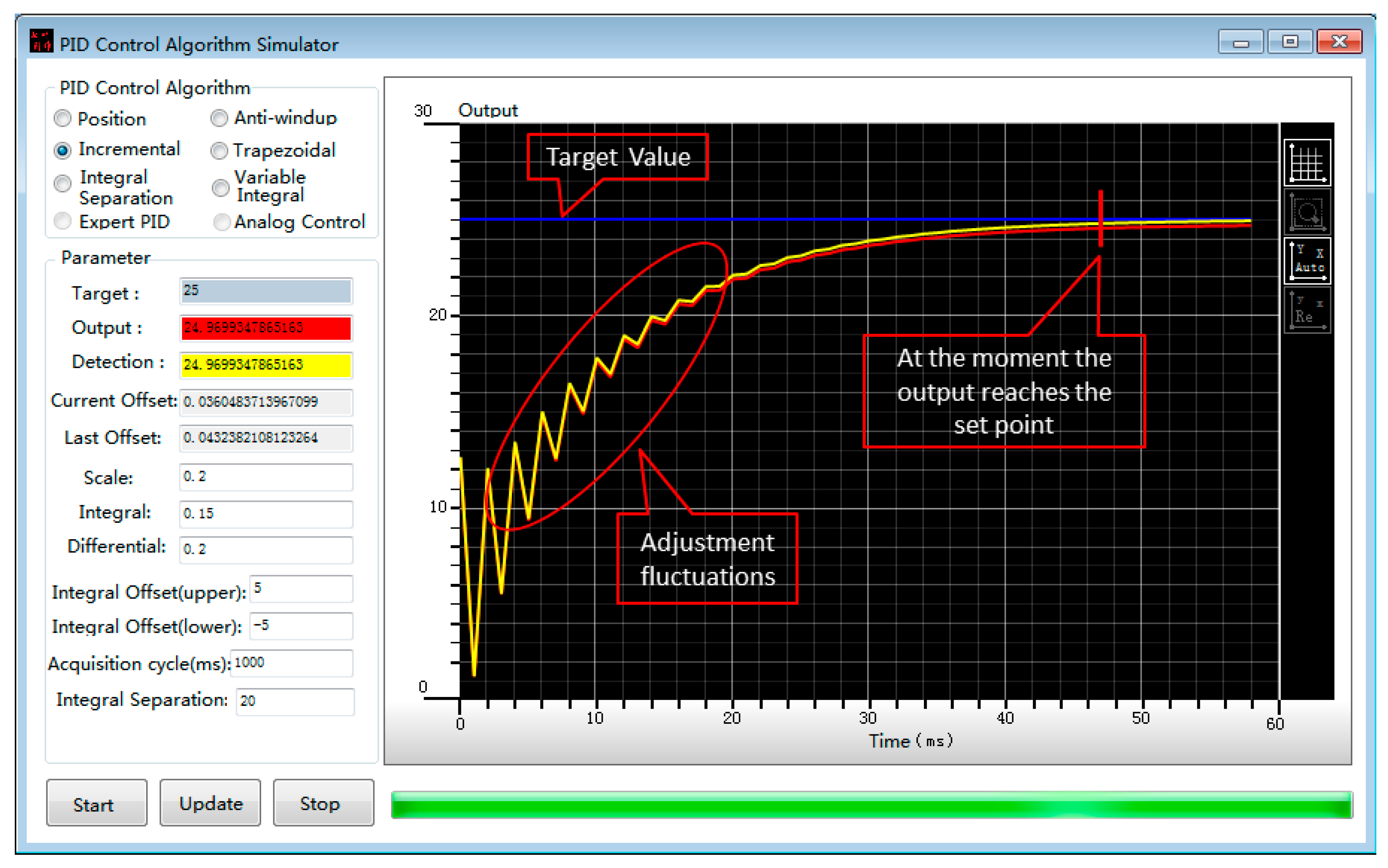
According to the observations on the PID control simulator, the effects of PID control before and after optimization are significantly different. Figure 9 shows the PID control simulation before optimization. The PID controllers usually have input data errors from sensor measurements. We used the input data errors directly in the calculation of differential coefficients. When calculating the integral values, we omitted the values if they were less than the precision. In Figure 9, there is no filtering value for the differential before optimization. The PID adjustment process uses the differential coefficients, resulting in the fluctuations of the PID output values with deviations. At the same time, in the integral calculation, the convergence adjustment speed of PID is not sensitive enough because of the omission of the integral terms that are less than the precision value.
Figure 10 shows PID control simulation after optimization. When calculating the differential optimization, the input filter of the cooling control value is the average of cooling deviations of the samples in the past four cycles. The control differential values are formed by weighted summation (as shown in Equation (19)). When an integral area is less than the output accuracy, the calculation of the integral needs to accumulate many of them to get the integral value.
Figure 9 and Figure 10 show that, in the same environment and with the same parameter settings, it takes 45 s to adjust the PID controller from the current temperature to the set value before optimization. After optimization, it takes only 20 s to reach the set temperature, which can greatly shorten the time spent by the PID control of an air conditioner. Meanwhile, the output control curve shows that, in the control process of the PID adjustment of an air conditioner, the optimized control output is more stable than that before optimization. The optimized control output can control an air conditioner effectively.
In the experiment of control optimization on cooling systems, we compared the traditional PID control model and the optimized PID control based on the dynamic predictive model. We carried out the experimental analysis from the following two aspects of temperature control and achieved energy efficiency optimization. Figure 11 shows the experimental results.
The first aspect is the temperature control of the building. According to the trend of temperature changes in Figure 11, although the traditional PID control can achieve the adaptive adjustment of temperatures, it has inadequate control on the cooling system due to the sudden changes of temperatures, which are caused by the load of the building. The temperature of the building is not stable enough. There would be locally overheated or undercooled situations. When using the optimization method of predictive model control, the temperature is more stable, temperature changes are more gradual, and the temperature distribution is more uniform. Table 5 includes the statistics of the temperatures of the building. It is up to 9.0 °C difference between the highest temperature and lowest temperature before control optimization. The temperature difference is within 3.0 °C after optimization.
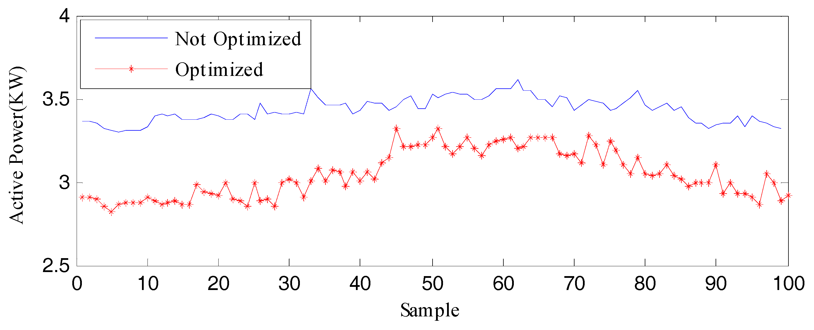
The second aspect of analysis is from the energy efficiency optimization. Figure 12 shows the statistics of energy consumption of the cooling system in the same time period. After optimization, the average energy consumption of the cooling system has also been reduced. Therefore, the predictive control model has a significant effect on reducing energy consumption of cooling systems.
In Table 6, before optimization, the cooling instantaneous power consumption is up to 3.48 KW; while the optimized instantaneous energy consumption is decreased by 0.17 KW. The deviation of the average energy consumption before and after optimization is 0.05 KW. Therefore, the predictive control model has a substantial effect on the optimization of energy efficiency for the cooling system. The total experiment time before and after optimization is 500 min each (5 min/sampling interval × 100 observations). The energy consumption is within 8 h (500/60 = 8.33) after the optimization. Each air conditioner can save nearly 9.4 KW of energy per day. The energy saving is up to 3416.4 KW per year. Therefore, the predictive control method has a substantial effect on the optimization of energy consumption for cooling systems.
6. Conclusions
This research presents a cooling control method based on MPC. The system is a coordinated proactive control method using dynamic time series prediction (PCM-DTSP) for sustainable facilities management (SFM). By integrating prediction results and monitored environmental data, the system is able to predict temperature changes and optimize controls. The PCM-DTSP helps to automate the functions of HVAC, particularly cooling systems, for improved energy efficiency. Specifically, the model makes substantial difference in terms of improved accuracy and timeliness in predicting cooling loads. If this system becomes widely used, it would considerably help buildings save energy and maintain sustainability. The modified MPC method with dynamic ESM in this research innovatively facilitates the study of dynamic service in control systems.
The experiment data show that the optimized cooling systems are more stable and consistent with a building’s cooling needs than the non-optimized systems. In addition, experiment tests verify that the optimized systems are able to reduce the power consumed by the cooling systems, stabilize the temperatures of the selected building, and reduce the energy consumption of the building.
However, one limitation of the control method is that its verification was performed on one building. The particular building was a closed-space modular building. The method developed in this research has potential to be used in open-space buildings. However, the thermodynamics of such a confined space should be used with caution when directly translated to other types of buildings. In future research, this dynamic ESM could be employed with machine learning to make the control of air conditioning systems more intelligent. Another possible future effort is to improve the prediction model by integrating other data sources.
Acknowledgments
This research work was supported by the Education Department of Shaanxi Province (17JZ047); the Special Foundation for Young Scientists of Xi’an University of Architecture and Technology (6040516148); and the Talent Technology Foundation of Xi’an University of Architecture and Technology (6040300613).
Author Contributions
Shunling Ruan and Haiyan Xie conceived and designed the experiments; Song Jiang performed the experiments; Shunling Ruan and Haiyan Xie analyzed the data; Shunling Ruan contributed analysis tools; and Shunling Ruan and Haiyan Xie wrote the paper.
Conflicts of Interest
The authors declare no conflict of interest.
Appendix A
Figure A1a–d shows the experimental results of using the triple exponential smoothing prediction method to simulate and analyze temperature changes with the static smoothing coefficients taken as , , and , respectively. The following discussions compare the observations of the prediction results.
Figure A1.
Forecasting results of static exponential smoothing method: (a) comparison of forecast temperatures and actual data when ; (b) comparison of forecast temperatures and actual data when ; (c) comparison of forecast temperatures and actual data when ; and (d) comparison of forecast temperatures and actual data when .
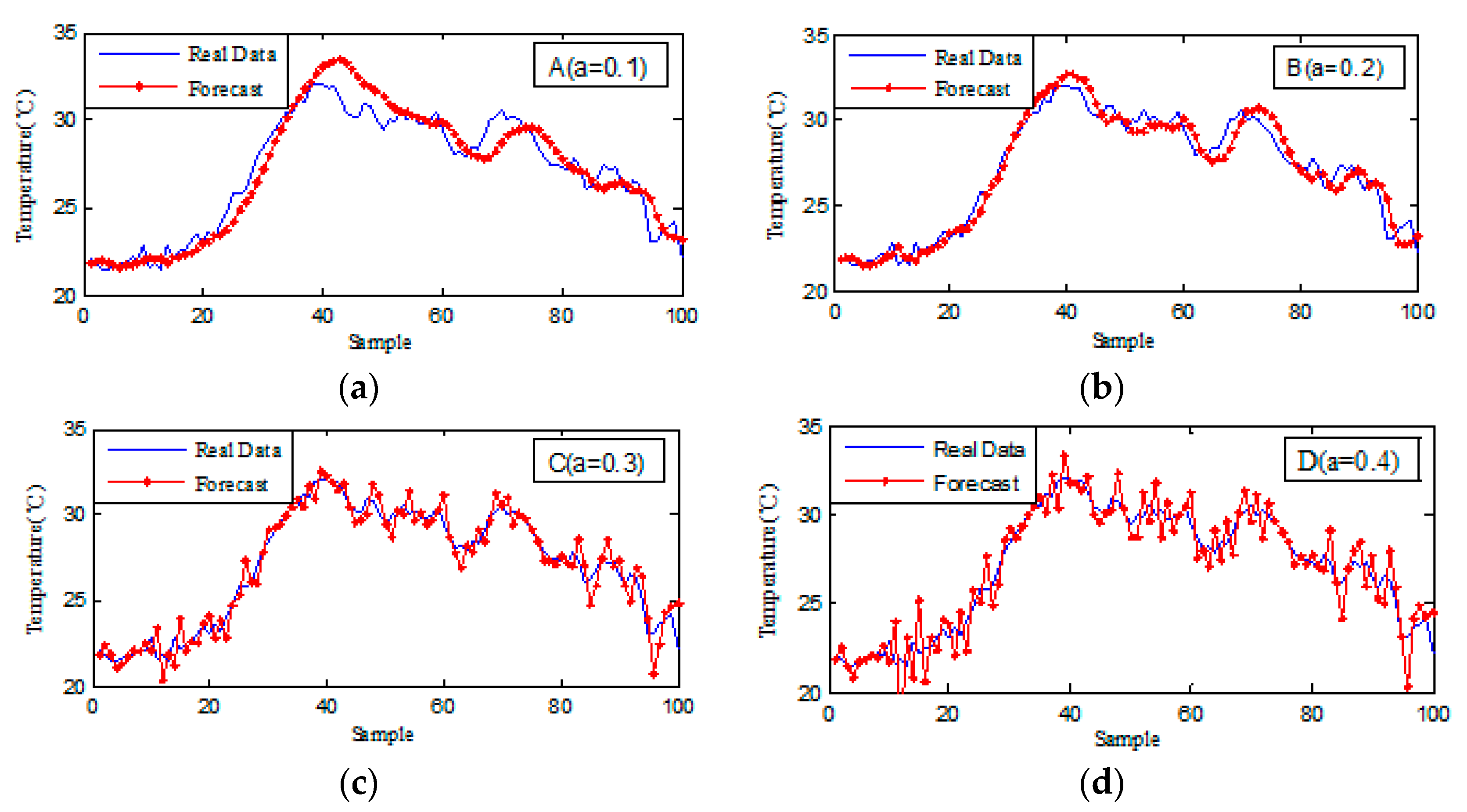
- When the smoothing coefficient , as shown in Figure A1a, the static exponential smoothing method can only predict the overall trend of the temperature changes. However, it cannot accurately predict the occurrences of sudden changes in temperatures. The deviations between the predicted results and the actual values are significant. Using the predicted results of this parameter to control cooling systems would lead to serious shortage of refrigeration or excessive cooling supply at a local area in a certain time range.
- When the smoothing coefficient , as shown in Figure A1b, relative to the situation when the smoothing coefficient , the accuracy of the forecast has greatly improved. The predicted results can reflect local variations of the temperatures. However, it has obvious lags between the predicted results and the actual data. It lacks sensitivity to temperature changes. Using this result to control cooling systems would cause local temperatures to be overheated or undercooled.
- When the smoothing coefficient , as shown in Figure A1c, the accuracy of the prediction is greatly improved. The prediction results can reflect local temperature variations. However, it has lags as well. If we use this result to control the cooling systems, it would create uneven cooling situations and waste energy consumption.
- When the smoothing coefficient , as shown in Figure A1d, the prediction results have strong jitters, where the peak values of the predicted results exceed the actual detections. If we follow these prediction results, it would exacerbate the phenomenon that the temperature is locally overheated or undercooled. It has a negative impact on the temperature stability. However, the sensitivity of the prediction algorithm is improved compared to the previous parameters.
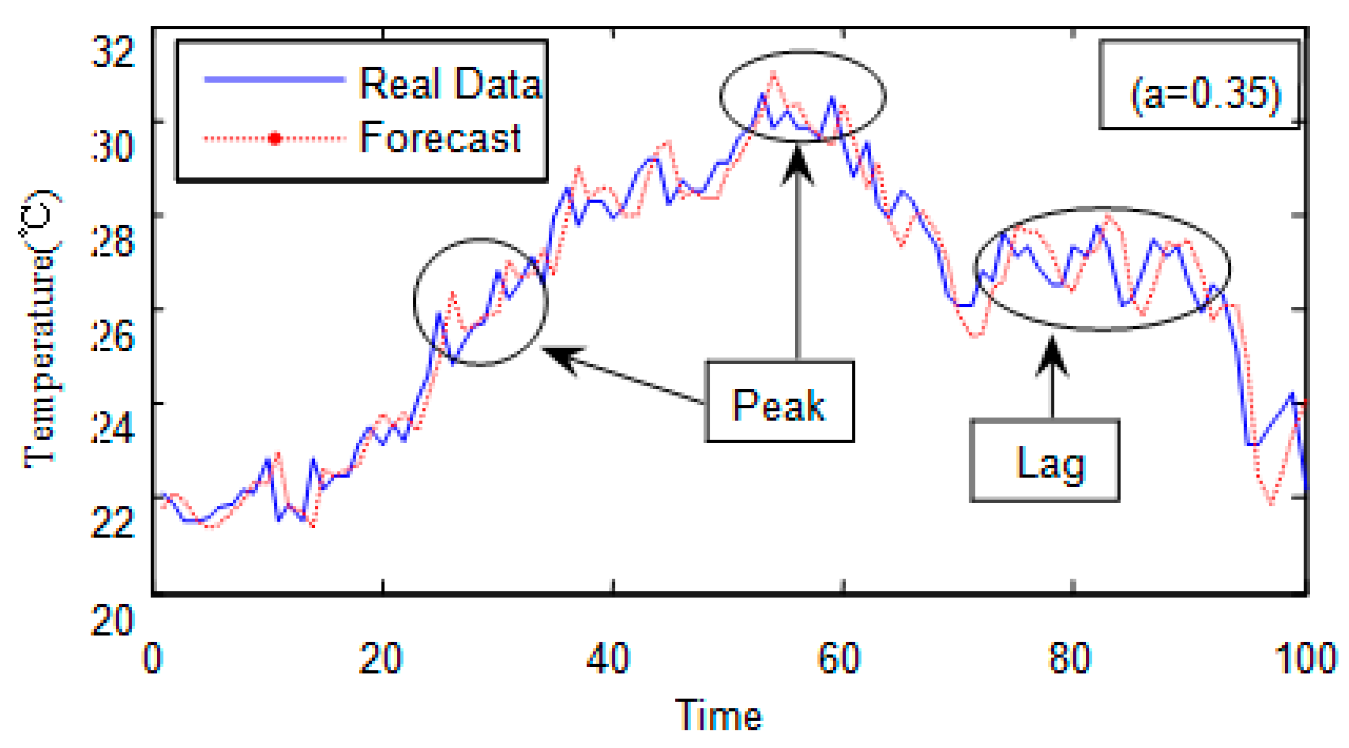
The above experimental and analytical results show that when the smoothing coefficient is 0.1 and 0.2, the sensitivity of the prediction algorithm is reduced. The algorithm cannot reflect short-term changes of the temperatures. When the smoothing coefficient is 0.3 and 0.4, the sensitivity of the prediction algorithm is greatly improved. When , the sensitivity of the prediction algorithm have lags in the region with large temperature fluctuation. However, the short-term forecast is improved. When , the hysteresis of the prediction algorithm is reduced. However, because the sensitivity is very high, predictions of peak temperatures tend to be much higher than the actual ones. Therefore, using the smoothing coefficient to simulate and analyze temperatures is appropriate. However, the smoothing coefficient should be between 0.3 and 0.4. In this research, we took as an example for experimental analysis. Figure A2 shows the results when the smoothing coefficient value is 0.35. The peak value of the temperature prediction is raised, but some of the predictions are still behind the original measured values.
Figure A2.
Forecasting results of static smoothing coefficient ().

The above analysis reveals that the static triple exponential smoothing predictive method can perform the basic prediction of the temperature trend of the building. However, the accuracy of prediction is not enough. Thus, in the rest calculation of the PCM-DTSP method, we did not use the static method.
References
- Gann, D.M.; Salter, A.J. Innovation in project-based, service-enhanced firms: The construction of complex products and systems. Res. Policy 2000, 29, 955–972. [Google Scholar] [CrossRef]
- Barrett, P. Achieving strategic facilities management through strong relationships. Facilities 2000, 18, 421–426. [Google Scholar] [CrossRef]
- Roper, K.O.; Payant, R.P. The Facility Management Handbook; AMACOM Div American Mgmt Assn: New York, NY, USA, 2014. [Google Scholar]
- Stark, J. Product lifecycle management. In Product Lifecycle Management (Volume 1); Springer: Berlin, Germany, 2015; pp. 1–29. [Google Scholar]
- Atkin, B.; Brooks, A. Total Facility Management; John Wiley & Sons: Hoboken, NJ, USA, 2014. [Google Scholar]
- Smith, L.G. Impact Assessment and Sustainable Resource Management; Routledge: Abingdon, UK, 2014. [Google Scholar]
- Higman, S. The Sustainable Forestry Handbook: A Practical Guide for Tropical Forest Managers on Implementing New Standards; Earthscan: London, UK, 2013. [Google Scholar]
- Shaikh, P.H.; Nor, N.B.M.; Nallagownden, P.; Elamvazuthi, I.; Ibrahim, T. A review on optimized control systems for building energy and comfort management of smart sustainable buildings. Renew. Sustain. Energy Rev. 2014, 34, 409–429. [Google Scholar] [CrossRef]
- Sherwin, D. A review of overall models for maintenance management. J. Qual. Maint. Eng. 2000, 6, 138–164. [Google Scholar] [CrossRef]
- Riley, D.R.; Varadan, P.; James, J.S.; Thomas, H.R. Benefit-cost metrics for design coordination of mechanical, electrical, and plumbing systems in multistory buildings. J. Constr. Eng. Manag. 2005, 131, 877–889. [Google Scholar] [CrossRef]
- Pérez-Lombard, L.; Ortiz, J.; Pout, C. A review on buildings energy consumption information. Energy Build. 2008, 40, 394–398. [Google Scholar] [CrossRef]
- Fantozzi, F.; Leccese, F.; Salvadori, G.; Rocca, M.; Garofalo, M. Led lighting for indoor sports facilities: Can its use be considered as sustainable solution from a techno-economic standpoint? Sustainability 2016, 8, 618. [Google Scholar] [CrossRef]
- Dekker, R. Applications of maintenance optimization models: A review and analysis. Reliab. Eng. Syst. Saf. 1996, 51, 229–240. [Google Scholar] [CrossRef] [Green Version]
- Márquez, A.C.; León, P.; Fernández, J.; Márquez, C.P.; Campos, M.L. The maintenance management framework: A practical view to maintenance management. J. Qual. Maint. Eng. 2009, 15, 167–178. [Google Scholar] [CrossRef]
- Avci, M.; Erkoc, M.; Rahmani, A.; Asfour, S. Model predictive hvac load control in buildings using real-time electricity pricing. Energy Build. 2013, 60, 199–209. [Google Scholar] [CrossRef]
- Ahuja, N.; Rego, C.; Ahuja, S.; Warner, M.; Docca, A. Data Center Efficiency with Higher Ambient Temperatures and Optimized Cooling Control. In Proceedings of the 2011 27th Annual IEEE Semiconductor Thermal Measurement and Management Symposium, Semiconductor Thermal Measurement and Management Symposium (SEMI-THERM), San Jose, CA, USA, 20–24 March 2011; p. 105. [Google Scholar]
- Durand-Estebe, B.; Le Bot, C.; Mancos, J.N.; Arquis, E. Simulation of a temperature adaptive control strategy for an iwse economizer in a data center. Appl. Energy 2014, 134, 45–56. [Google Scholar] [CrossRef]
- Ham, S.-W.; Park, J.-S.; Jeong, J.-W. Research paper: Optimum supply air temperature ranges of various air-side economizers in a modular data center. Appl. Therm. Eng. 2015, 77, 163–179. [Google Scholar] [CrossRef]
- Hiroshi, E.; Hiroyoshi, K.; Hiroyuki, F.; Toshio, S.; Takashi, H.; Masao, K. Cooperative control architecture of fan-less servers and fresh-air cooling in container servers for low power operation. ACM Oper. Syst. Rev. 2014, 48, 34. [Google Scholar]
- Huang, W.; Allen-Ware, M.; Carter, J.B.; Elnozahy, E.; Hamann, H.; Keller, T.; Lefurgy, C.; Li, J.; Rajamani, K.; Rubio, J. Tapo: Thermal-aware power optimization techniques for servers and data centers. In Proceedings of the 2011 International Green Computing Conference and Workshops Green Computing Conference and Workshops (IGCC), Orlando, FL, USA, 25–28 July 2011; p. 1. [Google Scholar]
- Nada, S.A.; Elfeky, K.E.; Attia, A.M.A. Experimental investigations of air conditioning solutions in high power density data centers using a scaled physical model. Études expérimentales des solutions de conditionnement d’air dans des centres de données à forte densité électrique en utilisant une maquette. Int. J. Refrig. 2016, 63, 87–99. [Google Scholar]
- Ogawa, M.; Endo, H.; Fukuda, H.; Kodama, H.; Sugimoto, T.; Horie, T.; Maruyama, T.; Kondo, M. Cooling control based on model predictive control using temperature information of it equipment for modular data center utilizing fresh-air. In Proceedings of the 2013 13th International Conference on Control, Automation & Systems (ICCAS 2013), Gwangju, Korea, 20–23 October 2013; p. 1815. [Google Scholar]
- Oxley, M.A. Online resource management in thermal and energy constrained heterogeneous high performance computing. In Proceedings of the 2016 IEEE 14th International Conference on Dependable, Autonomic and Secure Computing, 14th International Conference on Pervasive Intelligence and Computing, 2nd International Conference on Big Data Intelligence and Computing and Cyber Science and Technology Congress(DASC/PiCom/DataCom/CyberSciTech), Auckland, New Zealand, 8–12 August 2016; Pasricha, S., Ed.; IEEE: Piscataway, NJ, USA, 2016; p. 604. [Google Scholar]
- Smolaks, M. Research: Precision Cooling Expected to Boom in APAC; DatacenterDynamics: London, UK, 2017. [Google Scholar]
- Thota, P.K.; Dani, A.P.; Luh, P.B.; Gupta, S. Cooling load forecasting for chiller plants using similar day based wavelet neural networks. In Proceedings of the 2015 International Conference on Complex Systems Engineering (ICCSE), Storrs, CT, USA, 9–11 November 2015; p. 1. [Google Scholar]
- Zhou, R.; Bash, C.; Wang, Z.; McReynolds, A.; Christian, T.; Cader, T. Data center cooling efficiency improvement through localized and optimized cooling resources delivery. In Proceedings of the ASME 2012 International Mechanical Engineering Congress & Expositio, Houston, TX, USA, 9–15 November 2012. [Google Scholar]
- Geels, F.W. The multi-level perspective on sustainability transitions: Responses to seven criticisms. Environ. Innov. Soc. Trans. 2011, 1, 24–40. [Google Scholar] [CrossRef]
- Ioppolo, G.; Cucurachi, S.; Salomone, R.; Saija, G.; Shi, L. Sustainable local development and environmental governance: A strategic planning experience. Sustainability 2016, 8, 180. [Google Scholar] [CrossRef]
- Dounis, A.I.; Caraiscos, C. Advanced control systems engineering for energy and comfort management in a building environment—A review. Renew. Sustain. Energy Rev. 2009, 13, 1246–1261. [Google Scholar] [CrossRef]
- Wang, S.; Ma, Z. Supervisory and optimal control of building hvac systems: A review. HVAC&R Res. 2008, 14, 3–32. [Google Scholar]
- Afram, A.; Janabi-Sharifi, F. Theory and applications of hvac control systems—A review of model predictive control (MPC). Build. Environ. 2014, 72, 343–355. [Google Scholar] [CrossRef]
- Zhou, Y.; Li, N.; Li, H.; Zhang, Y. Regression cloud models and their applications in energy consumption of data center. J. Electr. Comput. Eng. 2015, 2015, 143071. [Google Scholar] [CrossRef]
- Tarutani, Y.; Hashimoto, K.; Hasegawa, G.; Nakamura, Y.; Tamura, T.; Matsudax, K.; Matsuoka, M. Reducing power consumption in data center by predicting temperature distribution and air conditioner efficiency with machine learning. In Proceedings of the 2016 IEEE International Conference on Cloud Engineering (IC2E), Berlin, Germany, 4–8 April 2016; p. 226. [Google Scholar]
- Ahn, J.; Cho, S.; Chung, D.H. Analysis of energy and control efficiencies of fuzzy logic and artificial neural network technologies in the heating energy supply system responding to the changes of user demands. Appl. Energy 2017, 190, 222–231. [Google Scholar] [CrossRef]
- Zeigler, B.P.; Praehofer, H.; Kim, T.G. Theory of Modeling and Simulation: Integrating Discrete Event and Continuous Complex Dynamic Systems; Academic Press: Cambridge, MA, USA, 2000. [Google Scholar]
- Pelzeter, A. Sustainability in facility management. In Proceedings of the Implementing Sustainability-Barriers and Chances, Book of Abstracts, sb13 Sustainable Building Conference, Munich, Germany, 24–16 April 2013; pp. 24–26. [Google Scholar]
- Doty, S.; Turner, W.C. Energy Management Handbook; CRC Press: Boca Raton, FL, USA, 2004. [Google Scholar]
- Dodrill, K. Demand Dispatch—Intelligent Demand for a More Efficient Grid; U.S. Department of Energy, National Energy Technology Laboratory Smart Grid Implementation Team: Morgantown, WV, USA, 2011.
- Paris, B.; Eynard, J.; Grieu, S.; Talbert, T.; Polit, M. Heating control schemes for energy management in buildings. Energy Build. 2010, 42, 1908–1917. [Google Scholar] [CrossRef]
- Arnold, M.; Andersson, G. Model predictive control of energy storage including uncertain forecasts. In Proceedings of the Power Systems Computation Conference (PSCC), Stockholm, Sweden, 22–26 August 2011; pp. 24–29. [Google Scholar]
- Li, X.; Wen, J. Review of building energy modeling for control and operation. Renew. Sustain. Energy Rev. 2014, 37, 517–537. [Google Scholar] [CrossRef]
- Li, X.; Wen, J.; Bai, E.-W. Developing a whole building cooling energy forecasting model for on-line operation optimization using proactive system identification. Appl. Energy 2016, 164, 69–88. [Google Scholar] [CrossRef]
- Ni, J.; Bai, X. A review of air conditioning energy performance in data centers. Renew. Sustain. Energy Rev. 2017, 67, 625–640. [Google Scholar] [CrossRef]
- Bilal, K.; Malik, S.U.R.; Khan, S.U.; Zomaya, A.Y. Trends and challenges in cloud datacenters. IEEE Cloud Comput. 2014, 1, 10–20. [Google Scholar] [CrossRef]
- Yin, X.; Sinopoli, B. Adaptive robust optimization for coordinated capacity and load control in data centers. In Proceedings of the 2014 IEEE 53rd Annual Conference on Decision and Control (CDC), Los Angeles, CA, USA, 15–17 December 2014; pp. 5674–5679. [Google Scholar]
- Clarke, D.W.; Mohtadi, C.; Tuffs, P. Generalized predictive control—Part I. The basic algorithm. Automatica 1987, 23, 137–148. [Google Scholar] [CrossRef]
- Kassmann, D.E.; Badgwell, T.A.; Hawkins, R.B. Robust steady-state target calculation for model predictive control. AIChE J. 2000, 46, 1007–1024. [Google Scholar] [CrossRef]
- Qin, S.J.; Badgwell, T.A. A survey of industrial model predictive control technology. Control Eng. Pract. 2003, 11, 733–764. [Google Scholar] [CrossRef]
- Montgomery, D.C.; Jennings, C.L.; Kulahci, M. Introduction to Time Series Analysis and Forecasting; John Wiley & Sons: Hoboken, NJ, USA, 2015. [Google Scholar]
- Xu, Y.; Chen, B.; Hu, Z. Research for multi-sensor data fusion based on huffman tree clustering algorithm in greenhouses. Int. J. Embed. Syst. 2016, 8, 34–38. [Google Scholar] [CrossRef]
- Ledolter, J.; Abraham, B. Some comments on the initialization of exponential smoothing. J. Forecast. 1984, 3, 79–84. [Google Scholar] [CrossRef]
- Yaffee, R.A.; McGee, M. An Introduction to Time Series Analysis and Forecasting: With Applications of Sas® and Spss®; Academic Press: Cambridge, MA, USA, 2000. [Google Scholar]
- Levinson, N. The wiener (root mean square) error criterion in filter design and prediction. Stud. Appl. Math. 1946, 25, 261–278. [Google Scholar] [CrossRef]
- Willmott, C.J.; Matsuura, K. Advantages of the mean absolute error (MAE) over the root mean square error (RMSE) in assessing average model performance. Clim. Res. 2005, 30, 79–82. [Google Scholar] [CrossRef]
- Allen, D.M. Mean square error of prediction as a criterion for selecting variables. Technometrics 1971, 13, 469–475. [Google Scholar] [CrossRef]
- Cochrane, D.; Orcutt, G.H. Application of least squares regression to relationships containing auto-correlated error terms. J. Am. Stat. Assoc. 1949, 44, 32–61. [Google Scholar]
Figure 1.
Research Design.
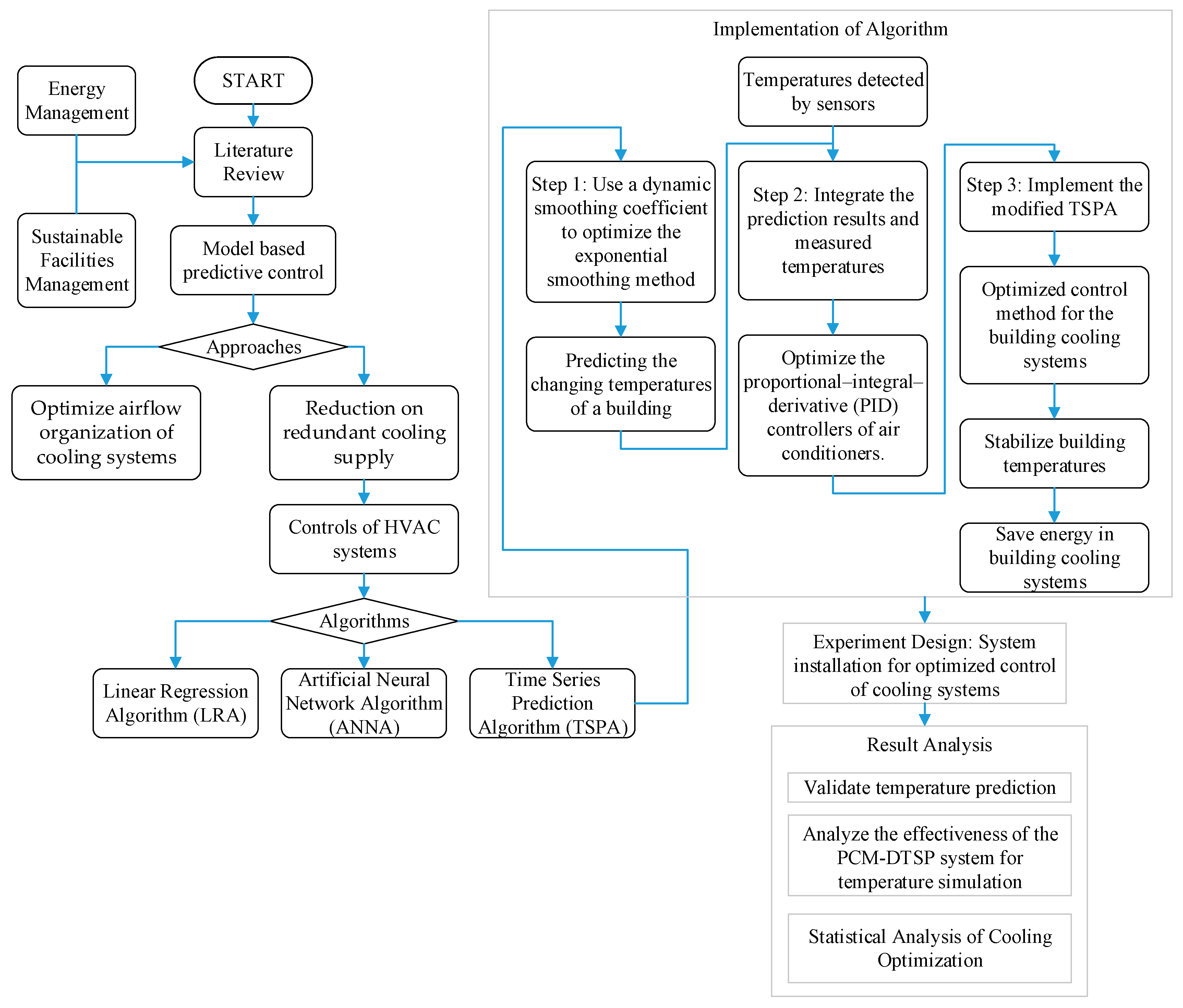
Figure 2.
Forecasting algorithm of Dynamic Time-Series Prediction (DTSP).

Figure 3.
The integration process of temperature prediction.

Figure 4.
Workflow of cooling optimized control with temperature predictions.
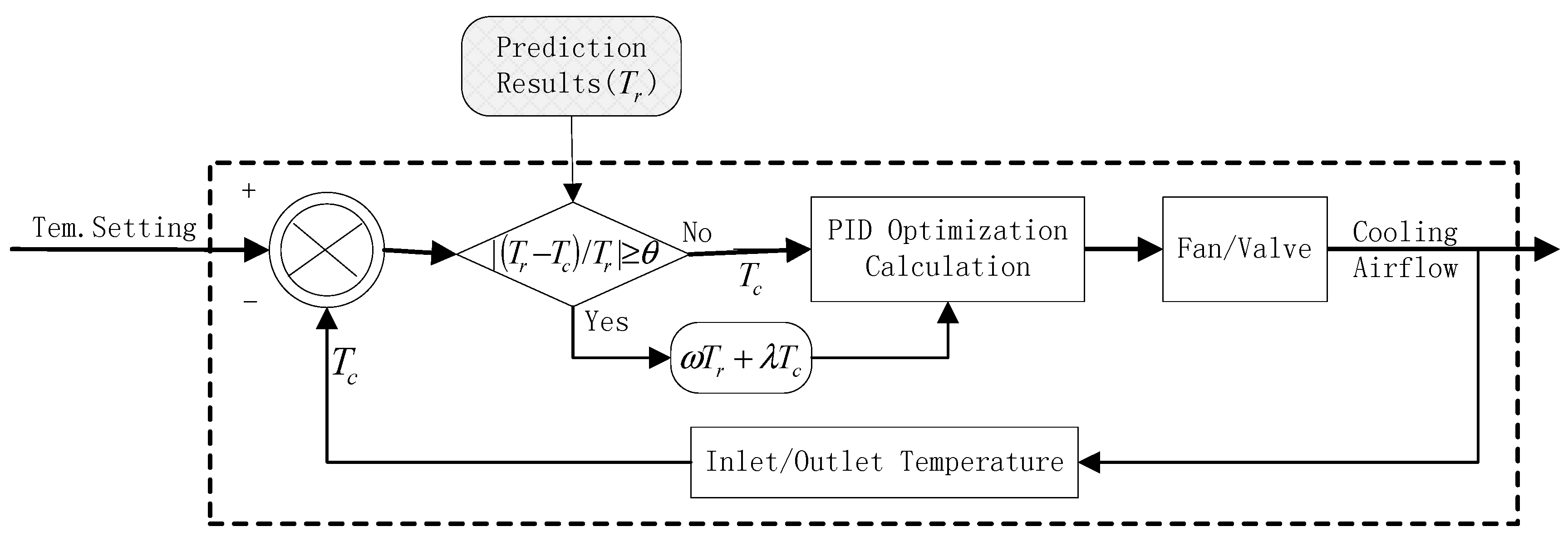
Figure 5.
The layout of the data center building for experiment design.

Figure 6.
Forecasting results of dynamic exponential smoothing method.

Figure 7.
Chart of dynamic smoothing coefficient changes (the smoothing coefficient is alpha or ).
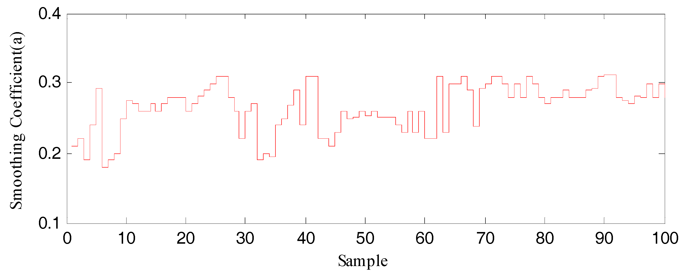
Figure 8.
Integration results of predicted temperature data from multiple sensors.

Figure 9.
Simulation results of PID control before optimization.

Figure 10.
Simulation results of PID control after optimization.
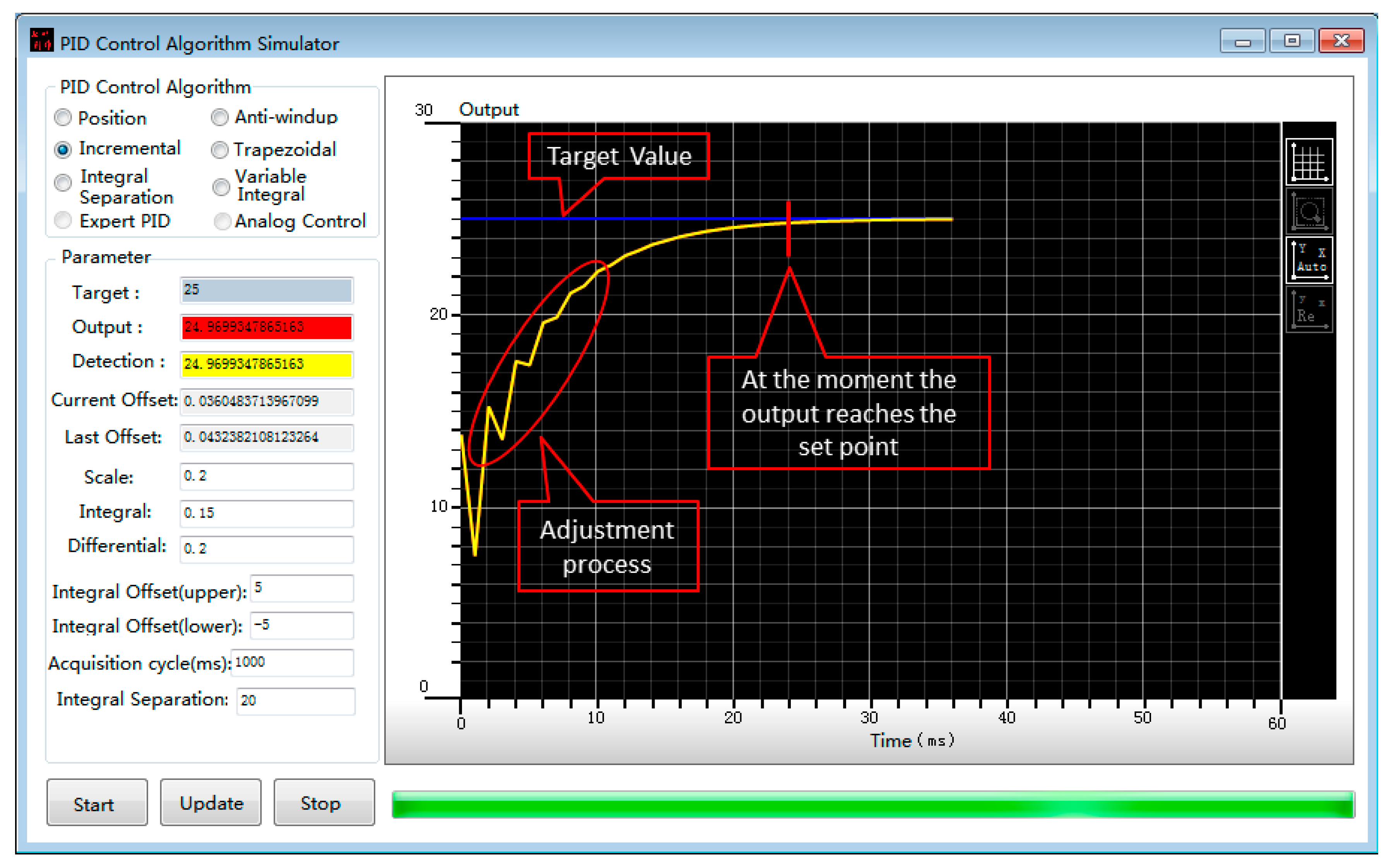
Figure 11.
Experimental Results of Temperature Based on Model Predictive Control (MPC).
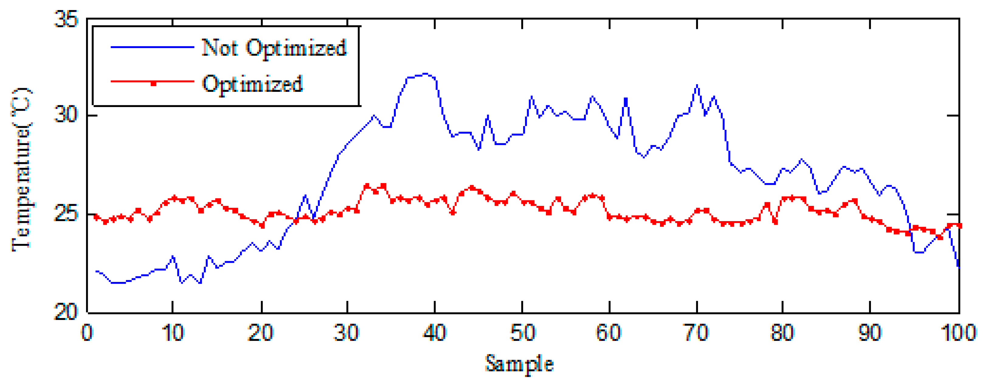
Figure 12.
Experimental Results of Cooling Consumption Based on MPC.

Table 1.
Comparison of Control Schemes of Energy Management.
| Type | Example | Feature | Limitations |
|---|---|---|---|
| Optimize airflow organization of cooling systems | Ham et al. [18] | Modular building; closed cold/hot channels to arrange airflow. | Low efficiency. |
| Ogawa et al. [22] | Natural-air cooling systems to reduce energy consumption | Easily affected by exterior temperatures. | |
| Hiroshi et al. [19] | Cooling control method based on the predictions of the thermal management requirements at a modular building. | Depended excessively on the air temperature of external environment; Low efficiency. | |
| Reduction on redundant cooling supply | Oxley et al. [23] | Improvement of computer room air conditioners (CRAC) for heterogeneous high-performance systems under thermal and energy constraints | Static method, especially when using templates generated offline to assist the online resource manager to make thermal-aware decisions based on the incoming workload and state of the HPC facility. Not been tested by real-world data. |
| Ogawa et al. [22] and Durand-Estebe et al. [17] | Optimize the controls of fan speeds. | Only gives the optimized approximating linear manifold in the configuration space represented by the data. | |
| Thota et al. [25] | Forecast cooling loads for temperature control; Similar day selection, wavelet decomposition, and neural networks; Different sub-bands (frequency components) and training a separate neural network for each component; | Neural networks cannot be retrained. If users add data later, it is almost impossible to add to an existing network. | |
| Huang et al. [20] | Determine the set points of CRAC based on the utilization level of the building. Applied a feedback-control approach on fans to achieve a trade-off between leakage power in circuit and fan power. | Failed to minimize the overall energy consumption of the systems and fans. | |
| Zhou et al. [26] | Localized and optimized cooling resources. Adaptive vent tiles mounted on floor and control cooling provisions to reduce costs. | Did not consider the power consumption of fans. | |
| Yin and Sinopoli [45] | Coordinated service provision with thermal-load awareness in job scheduling. | Very limited consideration on the dynamic features of cooling systems. |
Table 2.
Group Configuration for Analysis Temperature Integration.
| Cooling Equipment | Group | Group |
|---|---|---|
| Associated Sensor | ||
| Sensor Weights | ||
| Associated Server |
Table 3.
Examples of the integration analysis of temperature prediction results.
| Collection Time | Sensor | The Predicted Value at Different Cycles | Sensor Prediction (from Equation (14)) | Group Prediction (from Equation (15)) | |||
|---|---|---|---|---|---|---|---|
| 12 March 2017 08:12:10 | 23.5; 0.4 | 23.7; 0.3 | 23.8; 0.2 | 23.8; 0.1 | 23.65 | 23.58 | |
| 24.1; 0.4 | 24.0; 0.3 | 23.9; 0.2 | 23.8; 0.1 | 24.0 | |||
| 22.9; 0.4 | 23.0; 0.3 | 23.0; 0.2 | 23.1; 0.1 | 22.97 | |||
| 12 March 2017 08:17:21 | 23.8; 0.4 | 23.8; 0.3 | 23.9; 0.2 | 24.0; 0.1 | 23.84 | 23.71 | |
| 24.1; 0.4 | 24.0; 0.3 | 23.8; 0.2 | 23.8; 0.1 | 23.98 | |||
| 23.2; 0.4 | 23.2; 0.3 | 23.3; 0.2 | 23.4; 0.1 | 23.24 | |||
| 12 March 2017 08:22:05 | 23.8; 0.4 | 23.9; 0.3 | 23.9; 0.2 | 24.0; 0.1 | 23.87 | 23.70 | |
| 23.9; 0.4 | 23.8; 0.3 | 23.8; 0.2 | 23.7; 0.1 | 23.83 | |||
| 23.3; 0.4 | 23.4; 0.3 | 23.5; 0.2 | 23.6; 0.1 | 23.4 | |||
Table 4.
Proportional-Integral-Derivative (PID) control parameters of the controller.
| Parameter | Value | Parameter | Value |
|---|---|---|---|
| Temperature setting | 25 °C | Scale coefficient | 0.2 |
| Integral coefficient | 0.15 | Differential coefficient | 0.2 |
| Integral upper offset | 5 | Integral lower offset | −5 |
| Integral separation | 20 | Sampling period | 1000 ms |
Table 5.
Statistics of Temperature Maximum Deviation.
| Optimization | Avg. Temp. (°C) | Max. Temp. (°C) | Min. Temp. (°C) |
|---|---|---|---|
| Before | 28.6 | 30.6 | 21.5 |
| After | 26.3 | 26.7 | 23.3 |
Table 6.
Statistics of Cooling Energy Consumption.
| Optimization | Rated Power (kw) | Avg. Power(kw) | Max. Power (kw) | Min. Power (kw) |
|---|---|---|---|---|
| Before | 3.56 | 3.43 | 3.48 | 3.39 |
| After | 3.56 | 3.26 | 3.31 | 2.85 |
© 2017 by the authors. Licensee MDPI, Basel, Switzerland. This article is an open access article distributed under the terms and conditions of the Creative Commons Attribution (CC BY) license (http://creativecommons.org/licenses/by/4.0/).
Share and Cite
MDPI and ACS Style
Ruan, S.; Xie, H.; Jiang, S. Integrated Proactive Control Model for Energy Efficiency Processes in Facilities Management: Applying Dynamic Exponential Smoothing Optimization. Sustainability 2017, 9, 1597. https://doi.org/10.3390/su9091597
AMA Style
Ruan S, Xie H, Jiang S. Integrated Proactive Control Model for Energy Efficiency Processes in Facilities Management: Applying Dynamic Exponential Smoothing Optimization. Sustainability. 2017; 9(9):1597. https://doi.org/10.3390/su9091597
Chicago/Turabian StyleRuan, Shunling, Haiyan Xie, and Song Jiang. 2017. "Integrated Proactive Control Model for Energy Efficiency Processes in Facilities Management: Applying Dynamic Exponential Smoothing Optimization" Sustainability 9, no. 9: 1597. https://doi.org/10.3390/su9091597
Note that from the first issue of 2016, this journal uses article numbers instead of page numbers. See further details here.