Modeling Net Ecosystem Exchange for Grassland in Central Kazakhstan by Combining Remote Sensing and Field Data

Abstract
:1. Introduction
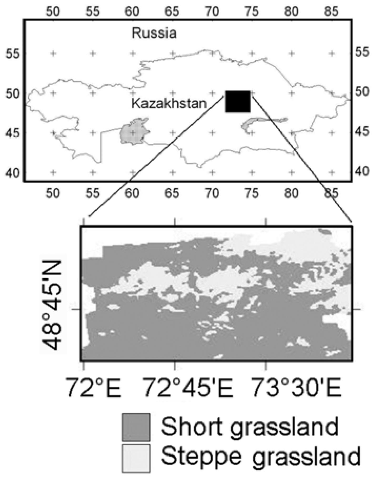
2. Study Area
3. Data
3.1. Field data
3.1.1. Carbon data

| Land cover | Dominate vegetation | Carbon, g/m² | |||
|---|---|---|---|---|---|
| BGB | AGBl | Litter | Total | ||
| Short grassland (8 sample plots) | Convolvulus arvensis, Artemisia sublessingiana | 38.1 | 54.2 | 80.5 | 172.8 |
| Steppe grassland (6 sample plots) | Festuca valesiaca, Stipa capillata, Coeleria cristata | 58.0 | 56.4 | 61.3 | 195.7 |
| Average of 14 sample plots | 48.0 | 61.6 | 70.9 | 179.5 | |
3.1.2. Vegetation structure variables
3.2. Satellite data
3.3. Climate data
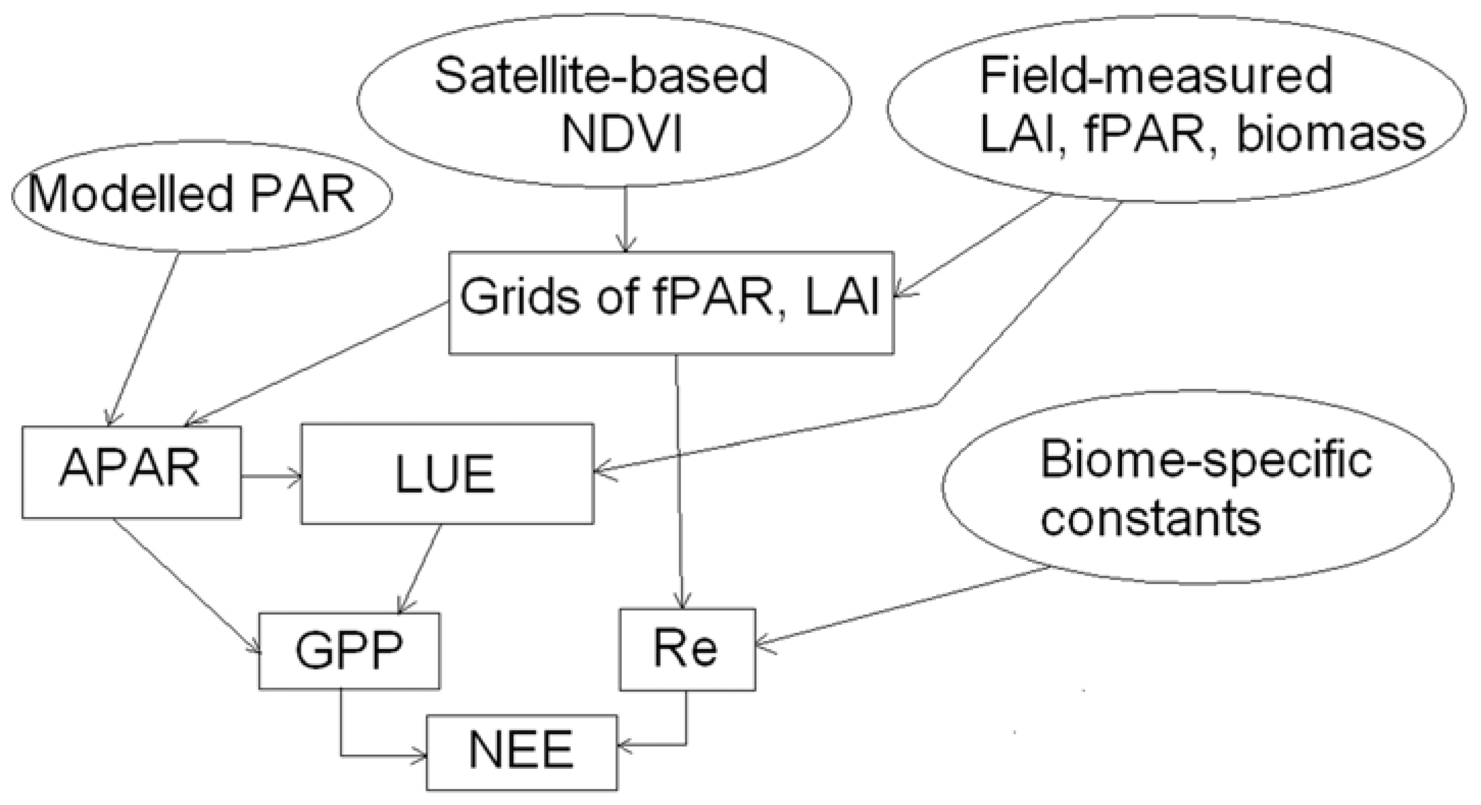
4. Methods

| Parameter | Units | Description | Land cover class | Source | |
|---|---|---|---|---|---|
| Short grassland | Steppe grassland | ||||
| LUEopt | gC/MJ | Optimum radiation conversion efficiency | 0.61 | 0.97 | This study |
| none | Temperature sensitivity factor | 2.0 | 2.0 | White et al. [37] | |
| °C | Base temperature | 20.0 | 20.0 | White et al. [37] | |
| SLA | m²/kg C | Specific leaf area | 40.0 | 40.0 | White et al. [37] |
| gC/gC/day | Maintenance respiration coefficient for fine roots at 20°C | 0.005 | 0.006 | White et al. [37] | |
| gC/gC/day | Maintenance respiration coefficient for above-ground plant parts at 20°C | 0.009 | 0.01 | White et al. [37] | |
| gC/gC | Growth respiration coefficient for fine roots | 0.3 | 0.3 | White et al. [37] | |
| gC/gC | Growth respiration coefficient for above-ground plant parts | 0.3 | 0.3 | White et al. [37] | |
| none | Carbon allocation fraction for fine roots | 1.0 | 1.0 | White et al. [37] | |
| none | Carbon allocation fraction for above-ground plant parts | 1.0 | 1.0 | White et al. [37] | |
| BGB/AGB1 | none | Ratio of below ground biomass to above ground biomass | 0.63 | 1.08 | This study |
| VPDstop | Pa | Vapour pressure deficit at photosynthesis stop | 5000 | 4100 | White et al. [37] |
| VPDstart | Pa | Vapour pressure deficit at photosynthesis start | 1000 | 970 | White et al. [37] |
| °C | Temperature at which LUE = LUEopt | 25.0 | 25.0 | White et al. [37] | |
| °C | Maximum temperature range | 40.0 | 40.0 | White et al. [37] | |
| F | gC/m²/day | Soil respiration rate at 0°C | 1.250 | 1.480 | Raich et al., [55]; Tesarova & Gloser, [62] |
4.1. PAR and APAR
4.2. fPAR and LAI
4.3. LUE
4.4. Modelling factors limiting light use efficiency
4.5. Modelling ecosystem respiration
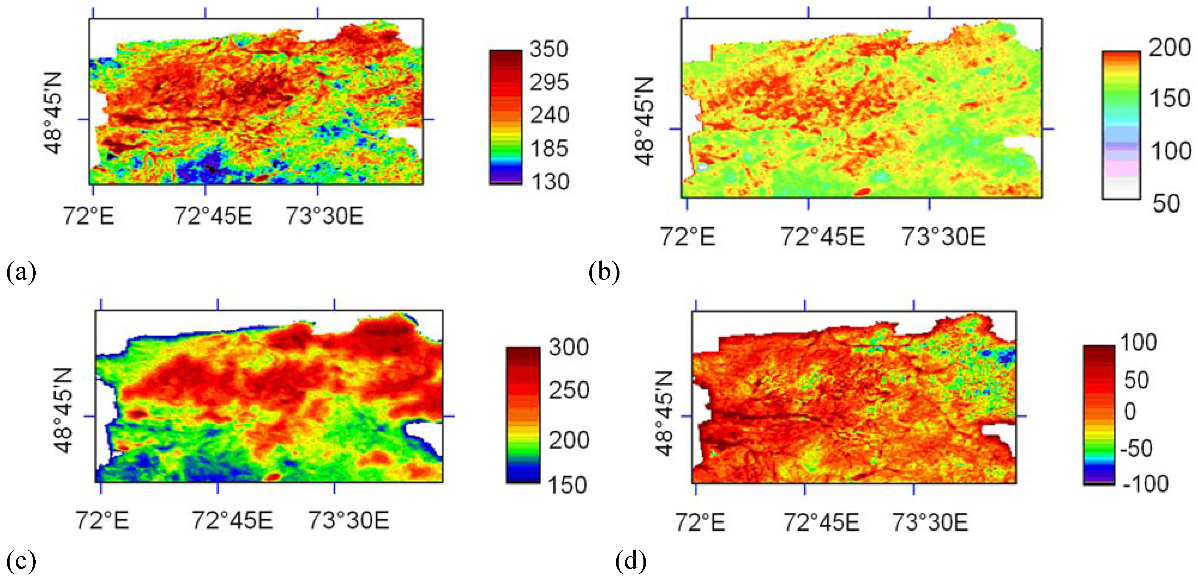
5. Results
5.1. Light use efficiency
5.2. Carbon sequestration
| Cover type | Area (km²) | Modelled variables | Mean (g C/m²/year) | Standard deviation | Total (g C×106) |
|---|---|---|---|---|---|
| Short grassland | 20,028 | GPP
NPP Re NEE | 211.03
131.30 187.05 13.17 | 51.42 44.29 35.12 32.03 | 4,226,509
2,629,877 3,446,237 263,768 |
| Steppe grassland | 6,955 | GPP
NPP Re NEE | 243.70
145.61 243.79 -0.09 | 59.50 54.22 44.47 39.56 | 1,694,934
1,012,648 1,695,351 -625 |
| Total | 26,983 | GPP
NPP Re NEE | 227.35
138.9 215.4 6.54 | 55.46 49.25 44.9 35.80 | 5,921,442
3,642,525 5,658,300 263,142 |
5.3. Evaluation of the modeling results
5.3.1. Qualitative comparison with previous studies
| Location and vegetation type | Estimating technique | GPP (gC/m²) | NPP(gC/m²) | NEP*(gC/m²) | Reference |
|---|---|---|---|---|---|
| Central Asia Dry steppe Dry steppe Dry steppe Semidesert Semidesert Semidesert Semidesert | Field observations | 326 126 148 90-310 117-189 220 114 | Pershina & Yakovlewa [28] Makarova [29] Tyurmenco [30] Robinson et al. [33] Tyurmenco [30] Fartushina [31] Gristchenco [32] | ||
| Former Czechoslovakia Grassland Grassland | Field observations | 664 492 | 481 318 | 18 21 | Tesarova & Gloser [62] Rychnovska et al. [63] |
| Global Grassland Grassland | Field observations | 70-410 91-385 | Zheng et al. [60] Rodin et al. [61] | ||
| Wyoming, USA Mixed-grass prairie Sagebrush steppe | Measurements of net ecosystem exchange | 321 239 | 14 42 | Hunt et al. [20] | |
| Sahel, Niger Grassland | Satellite-based LUE model | 352.1 | 169.3 | Seaquist et al. [19] | |
| Central Kazakhstan Dry steppe Semidesert | Satellite-based LUE model | 243.70 211.03 | 145.61 131.30 | -0.09 13.17 | The present study |
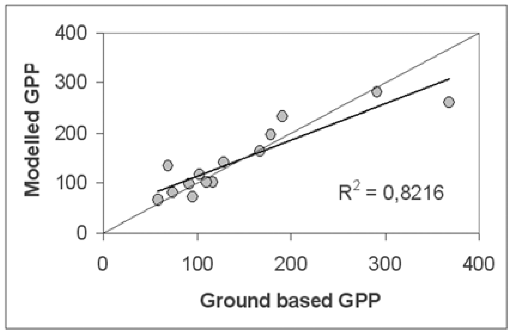
5.3.2. Direct comparison with ground-based data
The scale problem had been partly solved by a collection of several replicates at each test site. An average of these replicates for each test site was than computed.The ground surface at the most test sites and around them was relatively homogeny. We examined the homogeneity of the surface using a fine-resolution satellite image (Landsat ETM+) and considered that the variability of spectral reflection of the ground surface around the test sites was relatively low.
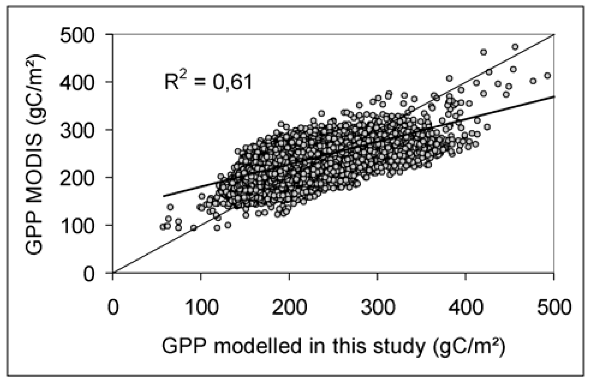
5.3.3. Comparison with MODIS GPP product

6. Discussion and Conclusions
Acknowledgments
References and Notes
- Heimann, M. Zonal distribution of terrestrial and oceanic carbon fluxes. Max-Planck Institute für Biogeochemie. Tech. Rep. 2001, 2, 27–29. [Google Scholar]
- Lal, R. Carbon sequestration in soils of Central Asia. Land Degrad. Develop. 2004, 15, 563–572. [Google Scholar] [CrossRef]
- Running, S.W.; Thornton, P.E.; Nemani, R. Global terrestrial gross and net primary productivity from the earth observing system. In Methods in Ecosystem Science; Sala, O.E., Jackson, R.B., Mooney, H.A., Howarth, R.W., Eds.; Springer-Verlag: New York, NY, USA, 2000; pp. 44–57. [Google Scholar]
- Sannier, C.A.; Taylor, J.C.; du Plessis, W.; Campbell, K. Realtime vegetation monitoring with NOAA AVHRR in Southern Africa for wildlife management and food security assessment. Int. J. Remote Sens. 1998, 19, 621–639. [Google Scholar] [CrossRef]
- Gower, S.T.; Kucharik, C.J.; Norman, J.M. Direct and indirect estimation of leaf area index, FAPAR, and net primary production of terrestrial ecosystems. Rem. Sens. Environ. 1999, 70, 29–51. [Google Scholar] [CrossRef]
- Lieth, H. Modelling the primary production of the world. In Primary Productivity of the Biosphere; Lieth, H., Whittacker, H., Eds.; Springer: Berlin, Germany, 1975; pp. 237–263. [Google Scholar]
- Woomer, P.L.; Toure, A.; Sall, M. Carbon stocks in Senegal’s Sahel transition zone. J. Arid Environ. 2004, 59, 499–510. [Google Scholar] [CrossRef]
- Potter, C.S.; Randerson, J.T.; Field, C.B.; Matson, P.A.; Vitousek, P.M.; Mooney, H.A.; Klooster, S.A. Terrestrial ecosystem production, a process model based on global satellite and surface data. Glob. Biogeochem. Cy. 1993, 7, 811–841. [Google Scholar] [CrossRef]
- Montheith, J.L. Climate and the efficiency of crop production in Britain. Philosoph. Trans. Royal Soc. London B 1977, 281, 277–294. [Google Scholar] [CrossRef]
- Field, C.B.; Randerson, J.T.; Malmström, C.M. Global net primary production, combining ecology and remote sensing. Rem. Sens. Environ. 1995, 51, 74–88. [Google Scholar] [CrossRef]
- Running, S.W.; Thornton, P.E.; Nemani, R. Global terrestrial gross and net primary productivity from the earth observing system. In Methods in Ecosystem Science; Sala, O.E., Jackson, R.B., Eds.; Springer-Verlag: New York, 2000; pp. 44–57. [Google Scholar]
- Turner, D.P.; Ollinger, S.V.; Kimball, J.S. Integrating remote sensing and ecosystem process models for landscape- to regional-scale analysis of the carbon cycle. BioScience 2004, 54, 573–584. [Google Scholar] [CrossRef]
- Heinsch, F.A.; Reeves, M.; Bowker, C.F. User’s quide, GPP and NPP (MOD 17A2/A3) products, NASA MODIS Land Algorithm. 2003. Available at: http//www.forestry.umt.edu/ntsg/.
- Goward, S.N.; Huemmrich, K.F. Vegetation canopy PAR absorptance and the normalized difference vegetation index, an assessment using the SAIL model. Remote Sens. Environ. 1992, 39, 119–140. [Google Scholar] [CrossRef]
- Goward, S.N.; Waring, R.H.; Dye, D.G.; Yang, J. Ecological remote sensing at OTTER, satellite macroscale observations. Ecol. Appl. 1994, 4, 322–343. [Google Scholar] [CrossRef]
- Running, S.W.; Nemani, J.M.; Glassy, J.M.; Thornton, P.E. MODIS daily photosynthesis and annual net primary production (NPP) product (MOD17), Algorithm Theoretical Basis, Document V. 3.0. 1999.
- Hunt, R.R.S.; Piper, R.; Newmani, C.D.; Keeling, R.D.; Running, S.W. Global net carbon exchange and intra-annual atmospheric CO2 concentrations predicted by an ecosystem process model and three-dimensional atmospheric transport model. Glob. Biogeochem. Cy. 1996, 10, 431–456. [Google Scholar] [CrossRef]
- Frouin, R.; Pinker, R.T. Estimating photosynthetically active radiation (PAR) at the earth’s surface from satellite observations. Remote Sens. Environ. 1995, 51, 98–107. [Google Scholar] [CrossRef]
- Seaquest, J.W.; Olsson, L. Rapid estimation of photosynthetically active radiation over the West African Sahel using the Pathfinder Land data set. JAG 1999, 1, 205–213. [Google Scholar] [CrossRef]
- Hunt, E.R.; Kelly, R.D.; Smith, W.K.; Fahnestock, J.T.; Welker, J.M.; Reiners, W.A. Estimation of carbon sequestration by combining remote sensing and net ecosystem exchange data for northern mixed-grass prairie and sagebrush-steppe ecosystems. Environ. Manage. 2004, 33, 432–441. [Google Scholar] [CrossRef]
- Justice, C.O.; Townshend, J.R.G.; Vermote, E.F.; Masuoka, E.; Wolfe, R.E.; Saleous, N.; Roy, D.P.; Morisete, J.T. An overview of MODIS land processing and product status. Remote Sens. Environ. 2002, 83, 3–15. [Google Scholar] [CrossRef]
- Seaquest, J.W.; Olsson, L.; Ardo, J. A remote sensing-based primary production model for grassland biomes. Ecol. Modell. 2003, 169, 131–155. [Google Scholar] [CrossRef]
- Friedl, M.A.; McIver, D.K.; Hodges, J.C.; Zhang, X.Y.; Muchoney, D.; Strahler, A.H.; Woodcock, C.E.; Gopal, S.; Schneider, A.; Cooper, A.; Baccini, A.; Gao, F.; Schaaf, C. Global land cover mapping from MODIS, algorithms and early results. Remote Sens. Environ. 2002, 83, 287–302. [Google Scholar] [CrossRef]
- Olofsson, P.; Eklundh, L.; Lagergren, F.; Jönsson, P.; Lindbroth, A. Estimating net primary production for Scandinavian forests using data from Terra/MODIS. Adv. Space Res. 2007, 39, 125–130. [Google Scholar] [CrossRef]
- Angell, R.T.; Svejcar, J.; Bates, N.; Saliendra, N.; Johnson, D. Bowen ratio and closed chamber carbon dioxide flux measurements over sagebrush steppe vegetation. Agr. Forest Meteorol. 2001, 108, 153–161. [Google Scholar] [CrossRef]
- Hanan, N.; Kabat, P.; Dolman, A.J.; Elbers, J.A. Photosynthesis and carbon balance of a Sahelian fallow savanna. Glob. Change Biol. 1998, 4, 523–538. [Google Scholar] [CrossRef]
- Chen, J.M.; Liu, J.; Cihlar, J.; Goulden, M.L. Daily canopy photosynthesis model through temporal and spatial scaling from remote sensing applications. Ecol. Modell. 1999, 124, 99–119. [Google Scholar] [CrossRef]
- Perschina, M.N.; Yakovlewa, M.E. Biologitcheskiy krugovorot w zone sukhich stepey SSSR. In Dokl. sov. potchwowedov k VII Mezschdunar. kongr. potchwowedov w USA; Moscow, AN SSSR, 1960; pp. 116–123. [Google Scholar]
- Makarowa, L.I. Tyrsovaya formacia w basseyne ozera Tchelkar. Materialy po flore i rastitelnosti Severnogo Prikaspiya. Leningrad, Wsesojuz. geogr. obstch. 1971, 5, 179–186. [Google Scholar]
- Tyurmenco, A.N. Biologitcheskiy krugovorot zolnych elementov pod celinnoy i culturnoy rastitelnostyu w zone sukhich i polupustynnych stepey. Genesis, swoystwa i plodorodiye potchw; Izd. Kazanskogo universiteta: Kazan, USSR, 1975; pp. 135–176. [Google Scholar]
- Fartuschina, M.M. Produktivnost rastitelnych associaciy pustynno-stepnogo complexa Severnogo Pricaspiya. Produktivnost senekosov i pastbistch; Nauka: Novosibirsk, USSR, 1986; pp. 74–77. [Google Scholar]
- Gristchenco, O.M. Podzemnaya phytomassa pyreynych limanov i eye rol w biologitchesom krugovorote westchestv i energii. Materialy o flore i rastitelnosti severnogo Pricaspiya. Leningrad, Wsesojuz. geogr. Obstch. 1972, 6, 54–68. [Google Scholar]
- Robinson, S.; Milner-Gulland, E.L.; Alimaev, I. Rangeland degradation in Kazakhstan during the Soviet-era, re-examining the evidence. J. Arid Environ. 2002, 53, 419–439. [Google Scholar] [CrossRef]
- Propastin, P.; Kappas, M. Reducing uncertainty in modelling NDVI-precipitation relationship, a comparative study using global and local regression techniques. GISci. Remote Sens. 2008, 45, 47–68. [Google Scholar] [CrossRef]
- Propastin, P.A.; Kappas, M.; Muratova, N. Inter-annual changes in vegetation activities and their relationship to temperature and precipitation in Central Asia from 1982 to 2003. J. Environ. Inf. 2008, 12, 75–87. [Google Scholar] [CrossRef]
- White, M.A.; Thornton, P.E.; Running, S.W.; Nemani, R.R. Parameterisation and sensitivity analysis of the BIOME-BGC terrestrial ecosystem model, net primary production controls. Earth Interact. 2000, 4, 1–85. [Google Scholar] [CrossRef]
- Norman, J.M.; Campbell, G.S. Canopy structure. In Plant Physiological Ecology, Field Methods and Instrumentation; Pearcy, R.W., Ehleringer, J., Mooney, H.A., Rundel, P.W., Eds.; Chapman and Hall: New York, NY, USA, 1989; pp. 301–325. [Google Scholar]
- Chen, J.M.; Cihlar, J. Plant canopy gap-size analysis theory for improving optical measurements of leaf area index. Appl. Opt. 1995, 34, 6211–6222. [Google Scholar] [CrossRef] [PubMed]
- Weiss, M.; Baret, F.; Smith, G.J.; Jonckheere, I.; Coppin, P. Review of methods for in situ leaf area index determination. Part II. Estimation of LAI, errors and sampling. Agr. Forest Meteorol. 2004, 121, 37–53. [Google Scholar] [CrossRef]
- Propastin, P.; Kappas, M. Mapping leaf area index in a semi-arid environment of Kazakhstan using fine-resolution satellite data and in situ measurements. GISci. Remote Sens. 2009, 46, 231–246. [Google Scholar]
- Tucker, C.J.; Sellers, P.J. Satellite remote sensing of primary vegetation. Int. J. Remote Sens. 1986, 7, 1395–1416. [Google Scholar] [CrossRef]
- Asrar, G.M.; Fuchs, M.M.; Kanemasu, E.T.; Hatfield, J.L. Estimating absorbed photosynthetically active radiation and leaf area index from spectral reflectance in wheat. Agronom. J. 1984, 87, 300–306. [Google Scholar] [CrossRef]
- Holben, B.N. Characteristics of maximum-value composite images from temporal AVHRR data. Int. J. Remote Sens. 1986, 7, 1417–1434. [Google Scholar] [CrossRef]
- Monteith, J.L.; Unsworth, M. Principles of environmental physics; Arnold: London, UK, 1990; pp. 112–114. [Google Scholar]
- Alisov, B.P.; Drosdow, O.A.; Rubinstein, E.S. Lehrbuch der Klimatologie; VEB Deutscher Verlag der Wissenschaften: Berlin, Germany, 1956. [Google Scholar]
- Myneni, R.B.; Nemani, R.R.; Running, S.W. Estimation of global LAI and fPAR from radiative transfer models. IEEE T. Geosci. Remote Sens. 1997, 35, 1380–1393. [Google Scholar] [CrossRef]
- Propastin, P.; Kappas, M. Mapping leaf area index over semi-desert and steppe biomes in Kazakhstan using satellite imagery and ground measurements. EARSEL eProc. 2009. (forthcoming). [Google Scholar]
- Goetz, S.J.; Prince, S.D. Modelling terrestrial carbon exchange and storage, evidence and implications of functional convergence light use efficiency. Adv. Ecol. Res. 1999, 28, 57–92. [Google Scholar]
- Kotchenova, S.Y.; Xiangdong, S.; Shabanov, N.V.; Potter, C.S.; Knyazikhin, Y.; Muneni, R.B. Lidar remote sensing for modelling gross primary production of deciduous forests. Remote Sens. Environ. 2004, 92, 158–172. [Google Scholar] [CrossRef]
- Lagergren, F.; Eklundh, L.; Grelle, A.; Lundblad, M.; Molder, M.; Lankreuer, H.; Lindroth, A. Net primary production and light conversion efficiency in a mixed coniferous forest in Sweden. Plant Cell Environ. 2005, 28, 412–423. [Google Scholar] [CrossRef]
- Turner, D.P.; Urbanski, S.; Bremer, D.; Wofsy, S.C.; Meyers, T.; Gower, S.; Gregory, M. A cross-biome comparison of daily light use efficiency for gross primary production. Glob. Change Biol. 2003, 9, 383–395. [Google Scholar] [CrossRef]
- Thornton, P.E. User’s Guide for BIOME-BGC, Version 4.1.1; Numerical Terradynamic Simulation Group, School of Forestry: University of Montana, Missoula, MT, USA, 2000. [Google Scholar]
- Ryan, M.G. A simple method for estimating gross carbon budgets for vegetation in forest ecosystems. Tree Physiol. 1991, 9, 255–266. [Google Scholar] [CrossRef] [PubMed]
- Raich, J.W.; Potter, C.S.; Bhagawati, D. Interannual variability in global soil respiration, 1980-94. Glob. Change Biol. 2002, 8, 800–812. [Google Scholar] [CrossRef]
- Saugier, B.; Roy, J.; Mooney, H.A. Estimation of global terrestrial productivity, converging toward a single number? In Terrestrial Global Productivity; Roy, J., Saugier, B., Mooney, H.A., Eds.; Academic Press: San Diego, CA, USA, 2001; pp. 543–557. [Google Scholar]
- Knapp, A.K.; Smith, M.D. Variation among biomes in temporal dynamics of aboveground primary production. Science 2001, 291, 481–484. [Google Scholar] [CrossRef] [PubMed]
- Richard, Y.; Poccard, I. A statistical study of NDVI sensitivity to seasonal and interannual rainfall variations in southern Africa. Int. J. Remote Sens. 1998, 19, 2907–2920. [Google Scholar] [CrossRef]
- Wang, J.; Price, K.P.; Rich, P.M. Spatial patterns of NDVI in response to precipitation and temperature in the central Great Plains. Int. J. Remote Sens. 2001, 22, 3827–3844. [Google Scholar] [CrossRef]
- Zheng, D.; Prince, S.; Wright, R. Terrestrial net primary production estimates for 0.5° grid cells from field observations – a contribution to global biogeochemical modelling. Glob. Change Biol. 2003, 9, 46–64. [Google Scholar] [CrossRef]
- Rodin, L.E.; Bazilevich, N.T.; Rozov, N.H. Productivity of the World’s Main Ecosystems; Natural Academy of Science: Washington, D.C., USA, 1975; pp. 13–26. [Google Scholar]
- Tesarova, M.; Gloser, J. Total CO2 outputs from alluvial soils with two types of grassland communities. Pedobiologia 1976, 16, 364–372. [Google Scholar]
- Rychnovska, M.; Ulehlova, B.; Jakrlova, J.; Tesarova, M. Biomass budget and energy flow in alluvial meadow ecosystem. In Proceedings of the XIII International Grassland Congress; Wojahn, E., Thöns, H., Eds.; Akademie Verlag: Berlin, DDR, 1980; Vol. 1, pp. 473–475. [Google Scholar]
- Fensholt, R.; Sandholt, I.; Rasmussen, M.S.; Stisen, S.; Diouf, A. Evaluation of satellite based primary production modelling in the semi-arid Sahel. Remote Sens. Environ. 2007, 105, 173–188. [Google Scholar] [CrossRef]
- Schaefer, K.; Denning, A.S.; Suits, N.; Kaduk, J.; Baker, I.; Los, S.; Prihodko, L. Effect of climate on interannual variability of terrestrial CO2 fluxes. Glob. Biogeochem. Cy. 2002, 16, 1102–1110. [Google Scholar] [CrossRef]
- Rasmussen, M.S. Developing simple, operational, consistent NDVI-vegetation models by applying environmental and climatic information. Part 1. Assessment of net primary production. Int. J. Remote Sens. 1998(a), 19, 97–111. [Google Scholar] [CrossRef]
- Rasmussen, M.S. Developing simple, operational, consistent NDVI-vegetation models by applying environmental and climatic information. Part 2. Crop yield assessment. Int. J. Remote Sens. 1998(b), 19, 119–139. [Google Scholar] [CrossRef]
- Rasmussen, M.S. Assessment of millet yields and production in Northern Burkina Faso using integrated NDVI from the AVHRR. Int. J. Remote Sens. 1992, 13, 3431–3442. [Google Scholar] [CrossRef]
- Prince, S.D. A model of regional primary production for use with coarse resolution satellite data. Int. J. Remote Sens. 1991(a), 12, 1313–1330. [Google Scholar] [CrossRef]
- Prince, S.D. Satellite remote sensing of primary production: comparison of results for Sahelian grasslands 1981-1988. Int. J. Remote Sens. 1991b, 12, 1301–1311. [Google Scholar] [CrossRef]
- Diallo, O.; Diouf, A.; Hanan, N.P.; Ndiaye, A.; Prevost, Y. AVHRR monitoring of savannah primary production in Senegal, West Africa. Int. J. Remote Sens. 1991, 12, 1259–1279. [Google Scholar] [CrossRef]
- Fensholt, R.; Sandholt, I.; Rasmussen, M.S. Validation of MODIS LAI, fPAR and the relation between fPAR and NDVI in a semi-arid environment using in situ measurements. Remote Sens. Environ. 2004, 91, 490–507. [Google Scholar] [CrossRef]
- Falge, E.; Tenhunen, J.; Baldocchi, D.; Aubinet, M.; Bakwin, P.; Berbigier, P.; Bernhofer, C.; Bonnefond, J.M.; Burba, G.; Clement, R.; Davis, K.J.; Elbers, J.A.; Falk, M.; Goldstein, A.H.; Grelle, A.; Granier, A.; Grunwald, T.; Gudmundsson, J.; Hollinger, D.; Janssens, I.A.; Keronen, P.A. Phase and amplitude of ecosystem carbon release and uptake potentials as derived from FLUXNET measurements. Agr. Forest Meteorol. 2002, 113, 75–95. [Google Scholar] [CrossRef]
- Propastin, P.; Kappas, M.; Erasmi, S.; Muratova, N.R. Remote sensing based study on intra-annual dynamics of vegetation and climate in drylands of Kazakhstan. Bas. Appl. Dryland Res. 2007, 2, 138–154. [Google Scholar]
© 2009 by the authors; licensee Molecular Diversity Preservation International, Basel, Switzerland. This article is an open-access article distributed under the terms and conditions of the Creative Commons Attribution license (http//creativecommons.org/licenses/by/3.0/).
Share and Cite
Propastin, P.; Kappas, M. Modeling Net Ecosystem Exchange for Grassland in Central Kazakhstan by Combining Remote Sensing and Field Data. Remote Sens. 2009, 1, 159-183. https://doi.org/10.3390/rs1030159
Propastin P, Kappas M. Modeling Net Ecosystem Exchange for Grassland in Central Kazakhstan by Combining Remote Sensing and Field Data. Remote Sensing. 2009; 1(3):159-183. https://doi.org/10.3390/rs1030159
Chicago/Turabian StylePropastin, Pavel, and Martin Kappas. 2009. "Modeling Net Ecosystem Exchange for Grassland in Central Kazakhstan by Combining Remote Sensing and Field Data" Remote Sensing 1, no. 3: 159-183. https://doi.org/10.3390/rs1030159