Aerosol Optical Depth Measured at Different Coastal Boundary Layers and Its Links with Synoptic-Scale Features

Abstract

This paper presents the results of measurements of aerosol optical properties which were made between 2006 and 2008 within the framework of various international projects in different locations such as Spitsbergen, northern Norway and Crete. The investigations were made under different baric topography conditions and in various seasons of the year which facilitated the investigations of spatial and temporal dependencies between upper troposphere mass state and spectral variations of aerosol properties. The results of aerosol optical depth (AOD) measurements showed significant episodes during which jet stream events (300 hPa surface) over the Arctic were present. The mean spectral characteristics of AOD from “before” and “after” the event differ by 0.14 versus the “during” phase of the episode. The macrometeorological relative topography charts shown also the relationships between the 500 hPa, close sea-level pressure SLP (1,000 hPa) charts surfaces and the attenuation caused by aerosol scattering and absorption in vertical profiles during the afternoon hours.

1. Introduction

Aerosol direct and indirect radioactive effects have been identified as key uncertainties for the prediction of the future global climate. To reduce these uncertainties several international field campaigns have been performed recently. These activities have focused on remote oceanic conditions (ACE 1), intermittently polluted marine environments (ACE 2, MINOS), highly polluted conditions (INDOEX), and continental conditions (LACE 98).

In coastal areas aerosols which are in the zone of direct interaction between the atmosphere and the ocean surface are characterized by fast temporal and spatial aerosol concentration changes. The spectrum of marine aerosol size distribution functions is complicated and depends strongly on weather conditions in the marine boundary layer, especially on wind speed, duration and direction as well as relative humidity. Additionally, it indirectly depends on the sources of aerosol generation and the air mass advection. The Arctic isentropic back trajectory method for synoptic types of identification was studied using the Arctic examples [1,2] and the European regions [3,4,5,6,7,8,9]. In order to analyze the impact of various meteorological conditions on aerosol optical parameters, including the aerosol optical depth in the boundary layer, the troposphere meteorological charts have been investigated.

The main motivation for such studies was the changes detected in the upper atmosphere during the SOAP experiment in Crete in 2006 where the backscatter LIDAR system was applied. These results were obtained in both the marine boundary layer and in the atmosphere column up to 5 km. It was also an impulse to further studies of manual analysis of meteorological forcing on aerosol optical depth. Similar studies have been performed with satellite observations [10,11,12,13] and meteorological analyses [14,15,16,17] also by using ground-based sun photometry and lidar on land or on the ship, plane platforms, which are very effective in investigations of aerosol optical properties [18,19,20,21,22,23,24,25,26,27,28,29,30,31,32]. Aerosol optical depth measured at different wavelengths is one of the key parameters in aerosol studies [33,34,35]. Atmospheric models need a reliable and easily obtainable indication of air mass characteristics in order to determine aerosol size distributions, concentrations and extinction in coastal areas, where a wide variety of rapidly changing atmospheric conditions have an impact on the aerosol ensemble. In this paper we would like to analyze the basic structure of aerosol optical depth in coastal atmosphere column and its connection with synoptic-scale features as relative topography charts, SLP chart and 300 hPa charts.

2. Description of Experiments and Instrumentation

The data presented in this paper were collected during three international measurement campaigns, SOAP, MACRON and AREX (Figure 1).

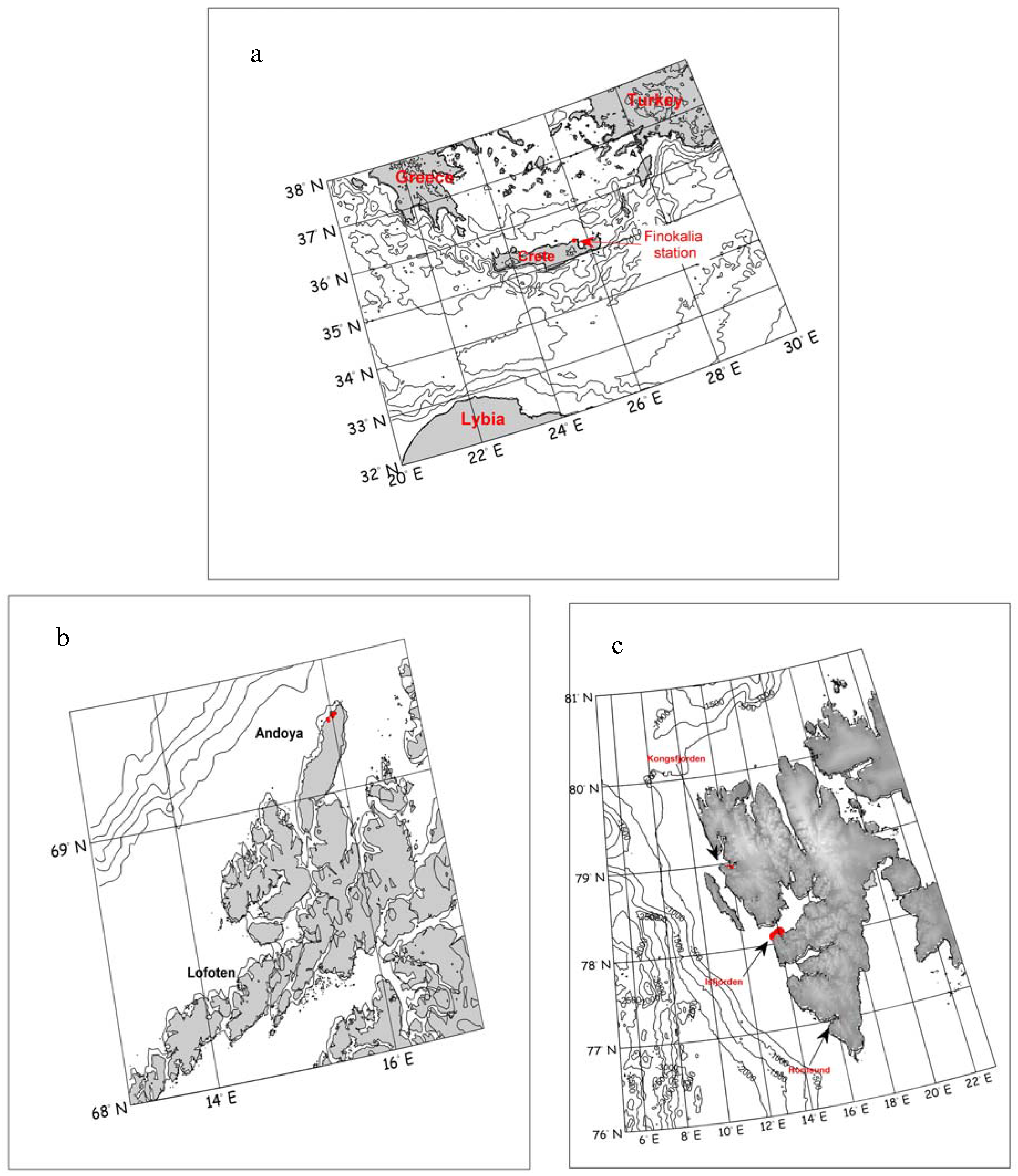
2.1. SOAP experiment in 2006

The Studies Of Aerosol Properties (SOAP) project which was part of the ACCENT program aimed at a determination of the direct aerosol climatic effect including solar radiative closure between observed and calculated aerosol properties. The scientific objectives of the project included:

• Determination of the vertical structure of the chemical, physical and optical properties of aerosol particles, including solar radiative closure between observed and calculated aerosol properties (direct climate effect).
• Using the above information to define the role of absorbing and non-absorbing aerosol particles in coastal regions.
• Improve the knowledge on aerosol particle life cycle and transport pathways across Europe, including the Saharan dust events.

Figure 1. Location of measurement stations: (a) Finokalia station during SOAP 2006. (b) Andoya Island during MACRON 2007. (c) Spitsbergen during AREX 2008.

Figure 1. Location of measurement stations: (a) Finokalia station during SOAP 2006. (b) Andoya Island during MACRON 2007. (c) Spitsbergen during AREX 2008.

The measurement campaign started on July 28 2006 using the lidar LB series provided by Raymetrics S.A. from Greece which was located at Finokalia station (35°20’N and 25°40’E) in Crete. Those were later supported by the measurements using the Microtops and a CIMEL CE-318 sun photometers. The full meteorological coverage (wind speed, direction, relative humidity, air temperature, etc.) was provided by the local meteo stations. Additionally, air mass backtrajectories were obtained for each selected day from the British Atmospheric Data Center. The campaign was completed on 9 August 2006.

2.2. MACRON experiment in 2007

The aim of the study was to estimate the emission of the marine aerosol by lidar and in-situ measurements. The program focused mainly on aerosol microphysical (size spectrum) and optical properties.

The use of the r/v Oceania facilitated the studies of sea spray emission from the sea surface. The vertical aerosol fluxes were calculated using experimental data on vertical gradients of aerosol concentration in the near-surface air layer collected with laser particle counters. Measurements were conducted in the 1 - 10 μm size range. Using vertical backscattering profiles collected from lidars located ashore, close to position of the vessel and irradiance measurements from photometers facilitated the estimation of vertical aerosol fluxes and aerosol size distributions in the entire boundary layer by using Microtops sun photometer.

In the first phase of the experiment (between 25 July and 5 August 2007) measurements of the optical properties of the atmosphere were performed. The measurements of optical properties of aerosol particles with multiwavelength lidars and passive photometers were made. ALOMAR tropospheric lidar and CIMEL sunphotometer, situated on the mountain top (380 m a.s.l.) provided additional information about the optical properties of the atmosphere in the upper part of the ABL and above it.

In the second phase of the experiment (between 6 and 15 August 2007) measurements with the lidars and the photometers were accompanied with laser particle counters (CSASP-100-HV-SP) providing aerosol particle concentrations and size distributions in the surface layer. Additional, meteorological, aerosol and optical measurements were performed from board of r/v Oceania sailing/anchored on the sea outside the breaker zone. The experiment was completed on 15 August.

2.3. AREX experiment in 2008

The aerosol studies during the ARctic EXperiment (AREX) 2008 were carried out onboard the r/v Oceania between June and late August 2008. During the campaign the vessel cruised for six weeks in the European Arctic between 0° E and 14° E and 69° N and 80° N. The aerosol studies were conducted using an ensemble of instruments, including laser particle counter CSASP-100-HV-SP (aerosol vertical size distributions) and Microtops II sun photometers. The laser particle counter was placed on a mast of the vessel and moved vertically, which facilitated the determination of the vertical structure of aerosol concentrations and their size distribution at altitudes of up to 20 m a.s.l., and sun photometers provided the AOD data. The full meteorological coverage (wind speed, direction, air mass backtrajectories, relative humidity, air temperature, etc.) was provided by the ship meteo station, which collected data every 10 seconds, from the British Atmospheric Data Center and using the HYSPLIT model. The location of the measurement stations beyond the Polar Circle are presented in Figure 1.

2.4. Description of selected instruments used during the campaigns

Measurements of Aerosol Optical Depth (AOD) were performed with hand-held Microtops II sun photometers and the Ozone Monitor. These instruments facilitated investigations of AOD at different wavelengths and were used at all locations (Table 1).

Table 1. Technical parameters of Microtops II sun photometers used during the studies.

Optical channels	340 ± 0.3 nm, 2 nm FWHM*
	380 ± 0.4 nm, 4 nm FWHM
	440 ± 1.5 nm, 10 nm FWHM
	500 ± 1.5 nm, 10 nm FWHM
	675 ± 1.5 nm, 10 nm FWHM
Resolution	0.01 W m−²
Dynamic range	>300000
Viewing angle	2.5°
Precision	1–2%
Non linearity	max. 0.002%

Table 1. Technical parameters of Microtops II sun photometers used during the studies.

Optical channels	340 ± 0.3 nm, 2 nm FWHM*
	380 ± 0.4 nm, 4 nm FWHM
	440 ± 1.5 nm, 10 nm FWHM
	500 ± 1.5 nm, 10 nm FWHM
	675 ± 1.5 nm, 10 nm FWHM
Resolution	0.01 W m−²
Dynamic range	>300000
Viewing angle	2.5°
Precision	1–2%
Non linearity	max. 0.002%

Single measurement “shots” were acquired over about 1 minute periods (in which measurements were made at all wavelengths, 10 second per channel: 340, 380, 440, 500, 675 nm) every 20 minutes. During the measurements the photographic documentation was made by using a CCD camera equipped with a wide-angle lens that was pointed on the solar target. The photos were used during further quality analyses.

The CIMEL Electronique 318A sunphotometer is a multi-channel, automatic sun-and-sky scanning radiometer that measures the direct solar irradiance and sky radiance at the Earth surface. Measurements are taken at pre-determined discrete wavelengths in the visible and near-IR parts of the spectrum to determine atmospheric transmission and scattering properties. A sensor head fitted with 25 cm collimators is attached to a 40 cm robot base which systematically points the sensor head at the sun (http://aeronet.gsfc.nasa.gov/new_web/system_descriptions.html).

Laser particle counter CSASP-100-HV is an optical spectrometer for aerosol measurements using the He-Ne laser. It measures particles of sizes from 0.5 to 48 μm in diameter at 36 ranges. Part of light scattered by aerosol particles which pass through the laser beam in the counter is directly a function of their sizes. Particles produce energy pulses when they cross the laser beam. These pulses are recorded by sensors, which determine two energy peaks (PMS, USA; http://www.pmeasuring.com).

In order to explain the most significant changes in coastal troposphere, it was necessary to use available weather charts from the following institutions: (1) GFS (Global Forecast System) Global Model from the "National Centers for Environmental Prediction" NCEP (http://www.ncep.noaa.gov/), (2) HYSPLIT (Hybrid Single Particle Lagrangian Integrated Trajectory Model, http://www.arl.noaa.gov/HYSPLIT.php), (3) San Francisco State University (SFSU)/Meteorology GFS Analysis (http://squall.sfsu.edu/), (4) http://www.wetter3.de/.

3. Theory

Signal of solar radiation passing through the atmosphere, in particular through the troposphere, is scattered (angular redistribution of energy) and absorbed (conversion of energy into either heat or photochemical change) on atmospheric aerosols, and gas particles. Value of this radiation is registered by the detector, and is described as follows:

$$I=I_0\exp \left[-{\displaystyle \underset{0}{\overset{\infty }{\int }}{\alpha }_{\lambda }\sigma dx}\right]=I_0\exp \left(-\tau \right)$$

(1)

where I₀ is solar irradiance at the top of atmosphere, I is solar irradiance after passing through the atmosphere, α_λσ is the extinction coefficient of the beam, x is the distance covered by the solar ray in the atmosphere [36] and τ_a is an expression for Aerosol Optical Depth as below:

$${\tau }_{\alpha }=[\ln I_0-\ln I-({\tau }_{Ray}\times m)\times (p/p_0)]/m$$

(2)

where τ_Ray is a part responsible for Rayleigh scattering (dependent from wavelength as well as τ_a) , p₀ is the pressure in standard atmosphere on the sea level, p is the local atmospheric pressure, m is the air mass and gaseous absorption is neglected [37].

Values of AOD at two different wavelengths allow us to receive the information about size distribution of aerosols in the troposphere, by using the Ångström coefficient α:

$$\alpha =-\frac{\ln \frac{{\tau }_{a,{\lambda }_1}}{{\tau }_{a,{\lambda }_2}}}{\ln \frac{{\lambda }_1}{{\lambda }_2}}$$

(3)

As τ_a for the larger wavelength approaches the τ_a for the smaller wavelength, larger particles dominate the spectrum and α gets smaller [38].

In order to asses the usefulness of data to further analysis we applied the turbidity factor as bellow:

τ_a,λ=βλ ^-α

(1)

which expresses the aerosol content of the atmosphere in the zenith direction, and is defined as the aerosol optical depth corresponding to a wavelength of 1 μm.

Supplementary manual analysis was also implemented to combine the aerosol optical depth with mid and high troposphere dynamics using the geostrophic approximation. Unlike in the boundary layer, friction force is negligible in the upper atmosphere so we can assume that the air flow is parallel to isohypses and the Coriolis force balances the horizontal pressure gradient that is perpendicular to isohypses from higher to smaller values as below:

$$\frac{\partial p}{\partial x}=\rho f\upsilon ;\frac{\partial p}{\partial y}=-\rho fu;\frac{\partial p}{\partial z}=-\rho g$$

(5)

where f = 2 Ω sinφ is the Coriolis parameter.

This simple dependence is applied only for the mid latitudes.

Another optical parameter for aerosol particles detecting was backscattering coefficient applied by means of laser remote-sensing techniques. The basic lidar equation is given by:

$$P(z)=P_0\frac{c\tau }{2}\beta (z)A_{tel}O(z)\frac{1}{z^2}\exp [-2{\displaystyle \underset{0}{\overset{z}{\int }}a(z*)dz*}]$$

(6)

where, P(z) is the detected backscattered radiation from range z, Po is the laser output power, τ is the laser pulse duration, c is the speed of light, β(z) is the volume backscatter coefficient, a(z) is the total atmospheric extinction coefficient, A_tel is the total telescope area and O(z) is the overlap function which takes into account geometrical and optical factors of the receiver arrangement [5]. The extinction term a (z) includes the contribution of the different absorbing atmospheric molecules, aerosol particles included [39].

4. Results and Discussion

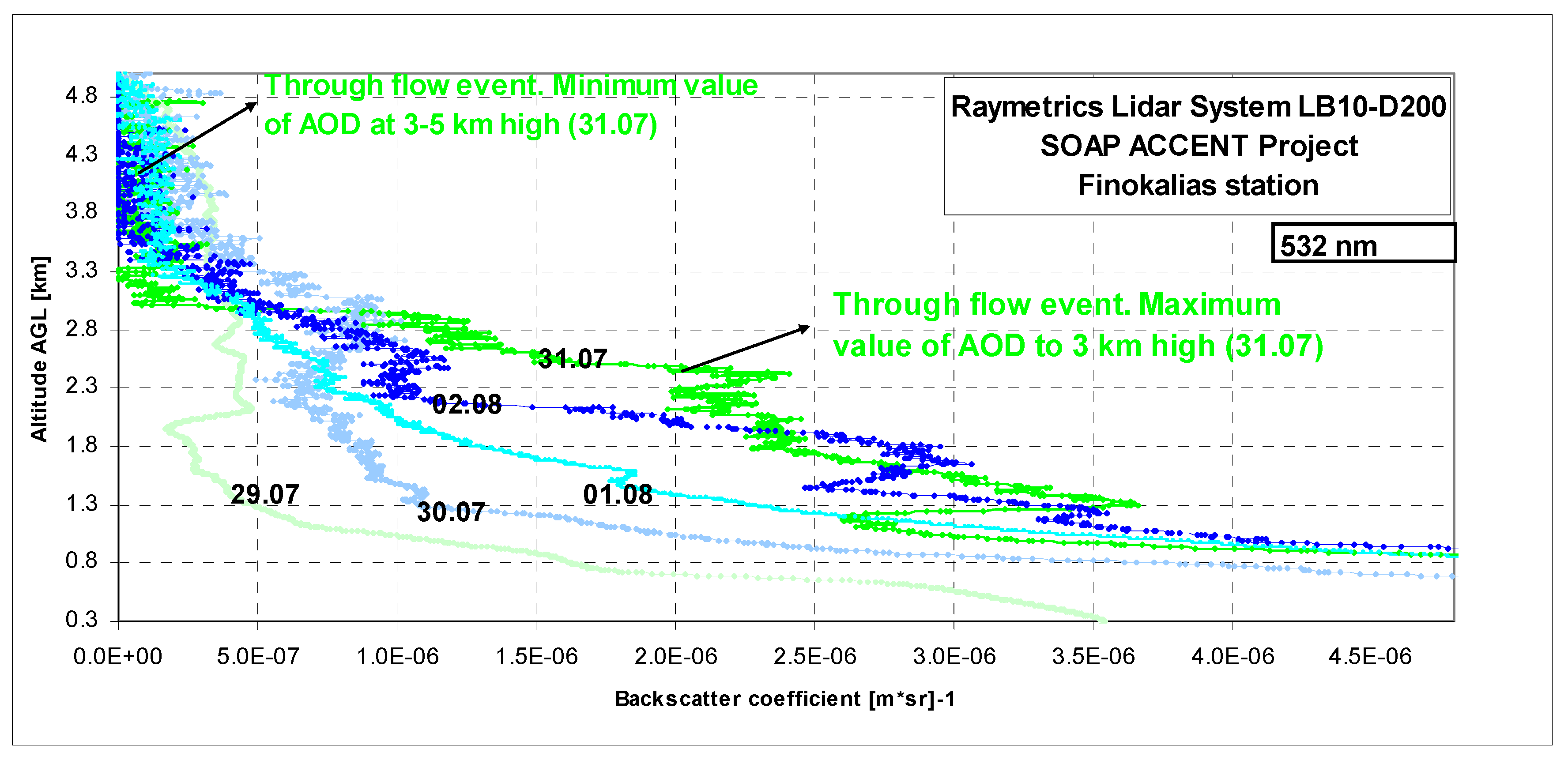
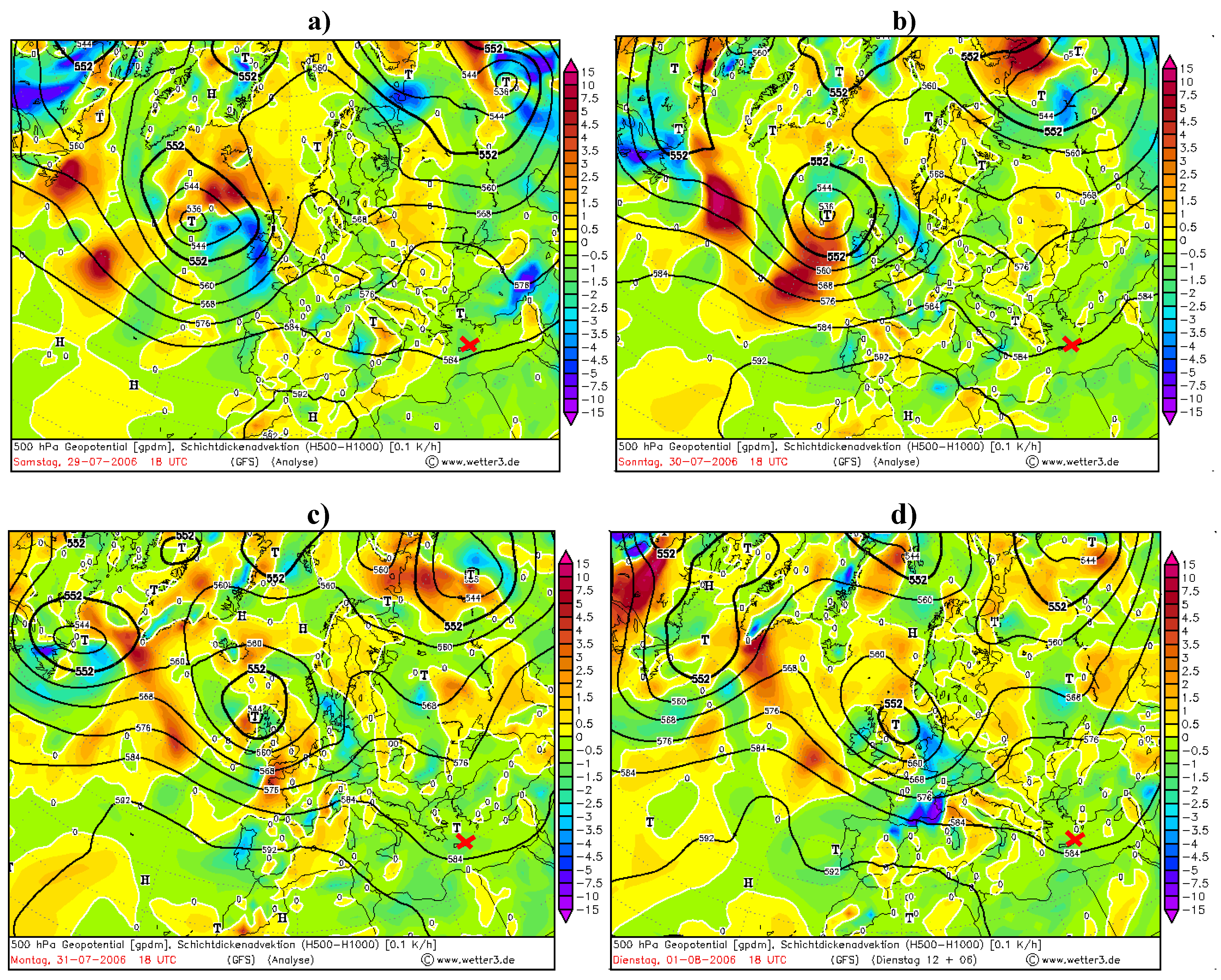
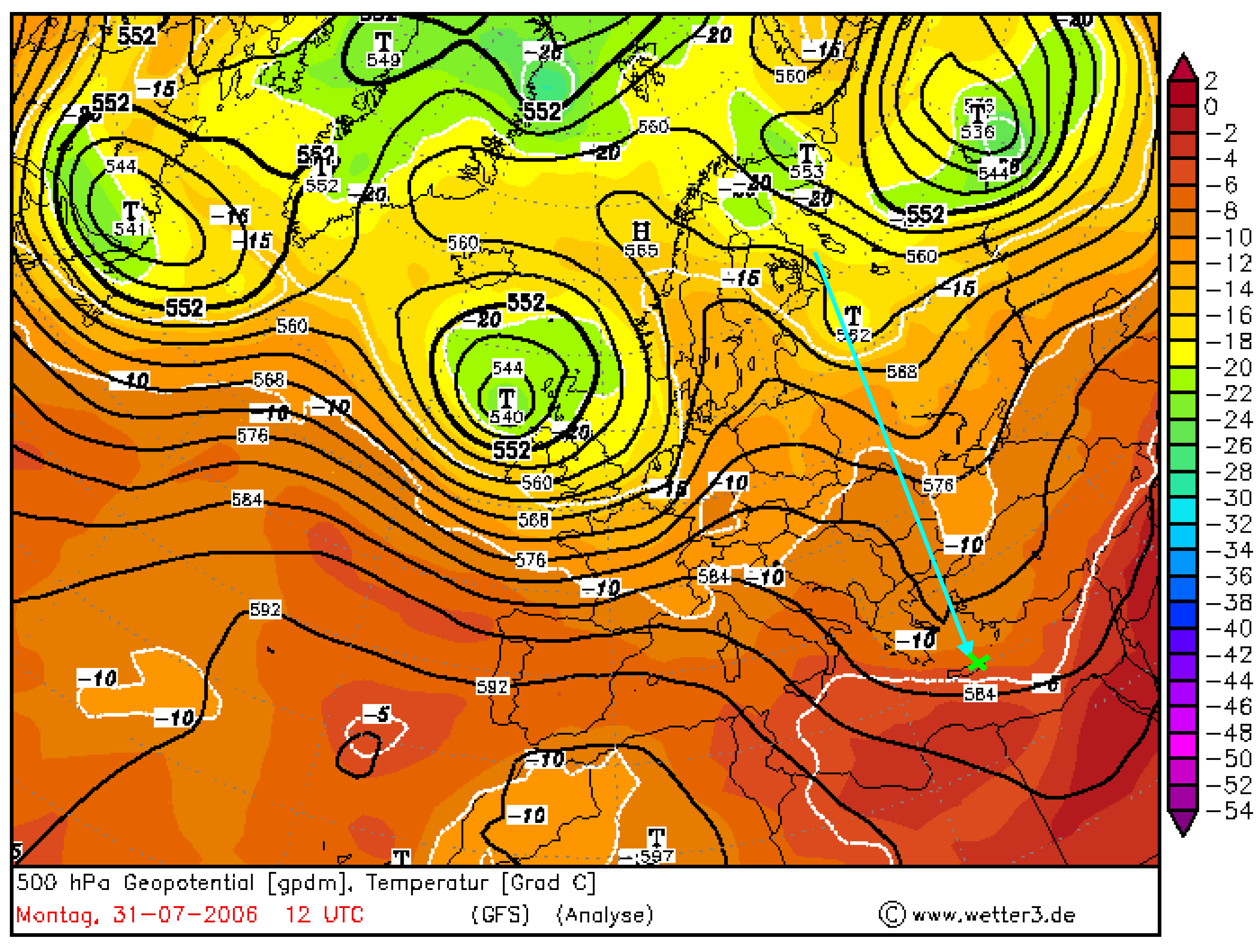
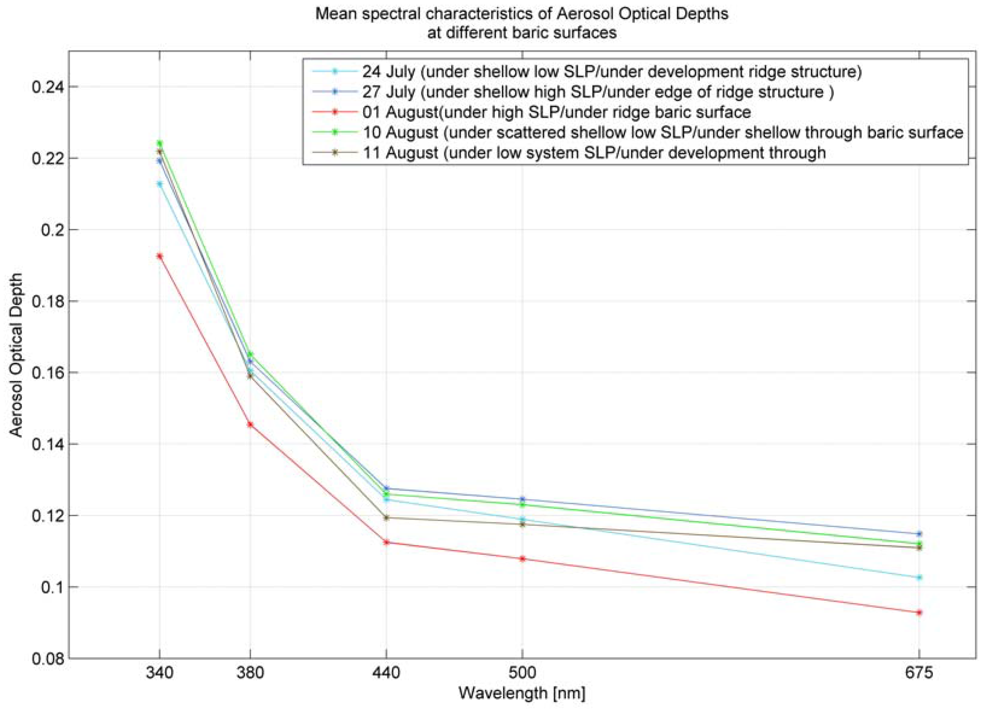
4.1. Mediterranean region

In order to find the relationships between the variability of aerosol motions in the upper level of marine air we compared our data with the pressure levels charts (in our case: 850, 700, 500 hPa) which showed the distribution of particular isobaric surface over sea level in gpdm – geopotential decameters. This unit reflects the height at which the constant pressure layer can be found. To review the measurement data and the state of the atmosphere data (baric topography charts) the laser data were analyzed.

As shown in Figure 2 the transmitted laser beam overlaps completely with the field of view at heights from over 300 m. This means that the data from the boundary layer were excluded from the analysis. The upper layer (from 300 m to 5 km) backscatter coefficient changed rapidly above 2.5 km during observation period. In this part of troposphere column turbulence and friction forces can be ignored and the main analyses are focused on atmospheric circulation patterns over the synoptic scale. This is directly combined with the source regions that can be pointed using the upper air chart analyses.

Figure 2. Backscatter coefficient obtained from lidar measurements during the SOAP experiment in Crete and its vertical structure. The data were collected day by day from 29 July to 2 August.

Figure 2. Backscatter coefficient obtained from lidar measurements during the SOAP experiment in Crete and its vertical structure. The data were collected day by day from 29 July to 2 August.

The most significant changes were observed on 29, 31 July and on 1 August. The analysis of relative topography charts can represent the thickness of the layer between the 500 hPa level and the 1,000 hPa. These levels represent the virtual isotherms for the layer 500/1,000 hPa [40] and can identify the advection of cold or warm air according to a simple relation between temperature and pressure in atmosphere layer 3–5 km:

• advection temperature decreasing is related with advection pressure decreasing
• advection temperature increasing is related with advection pressure increasing.

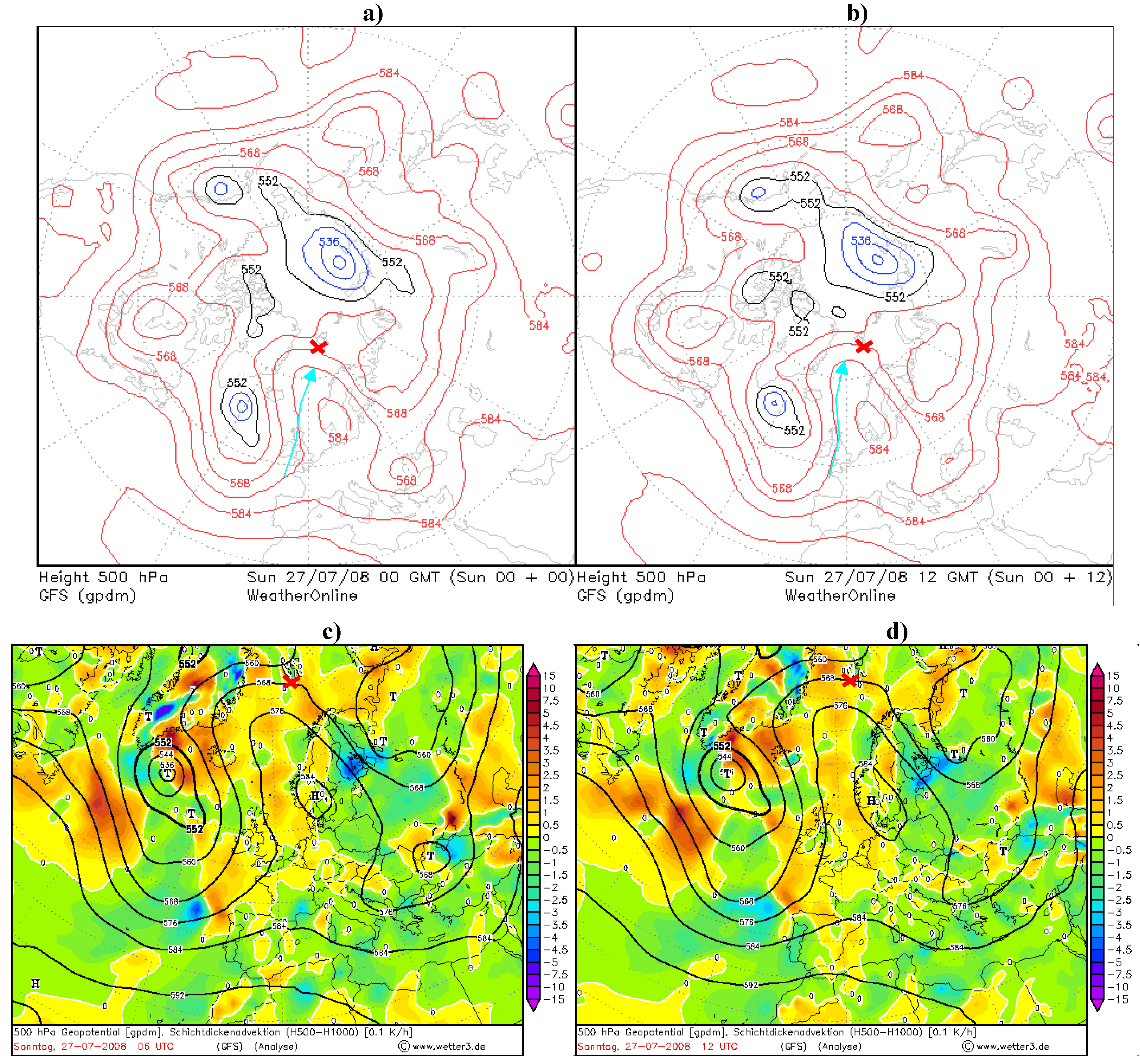
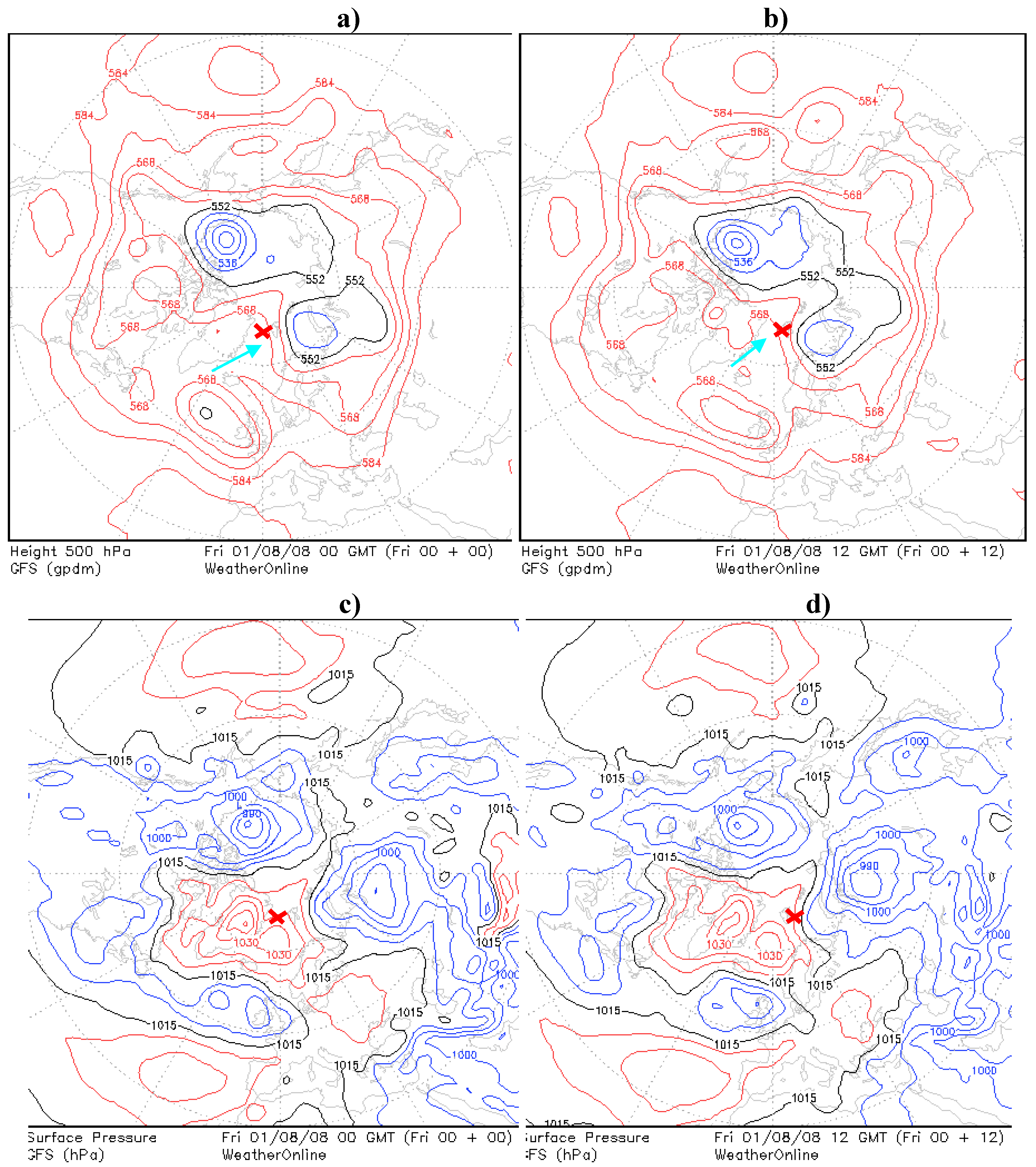
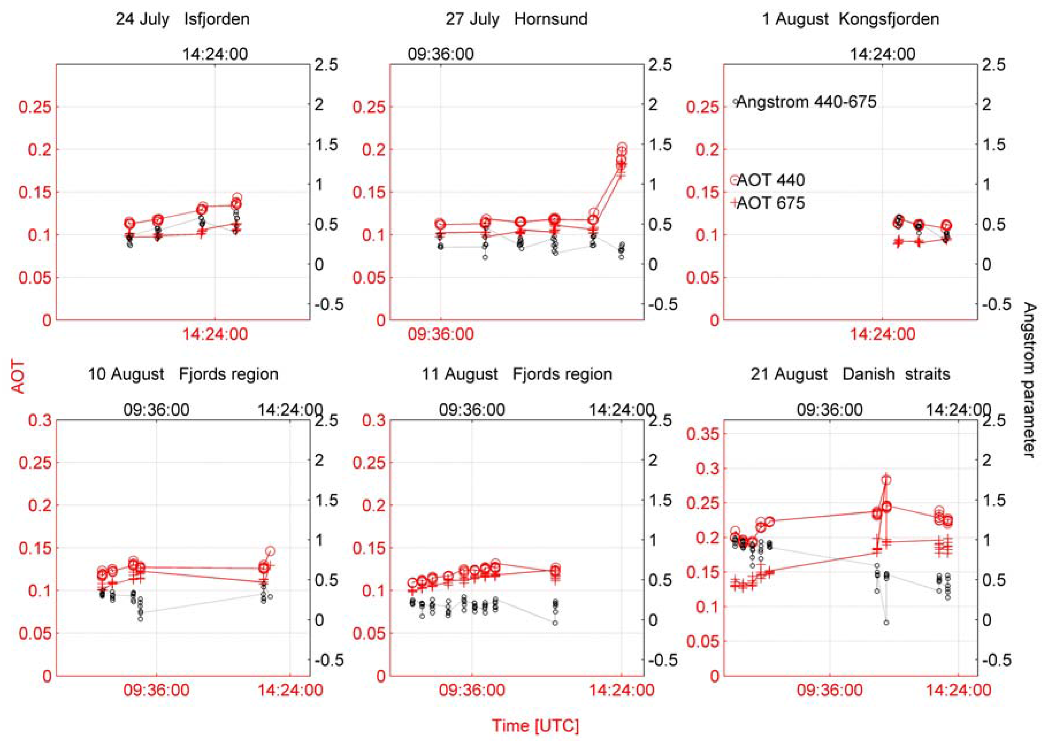
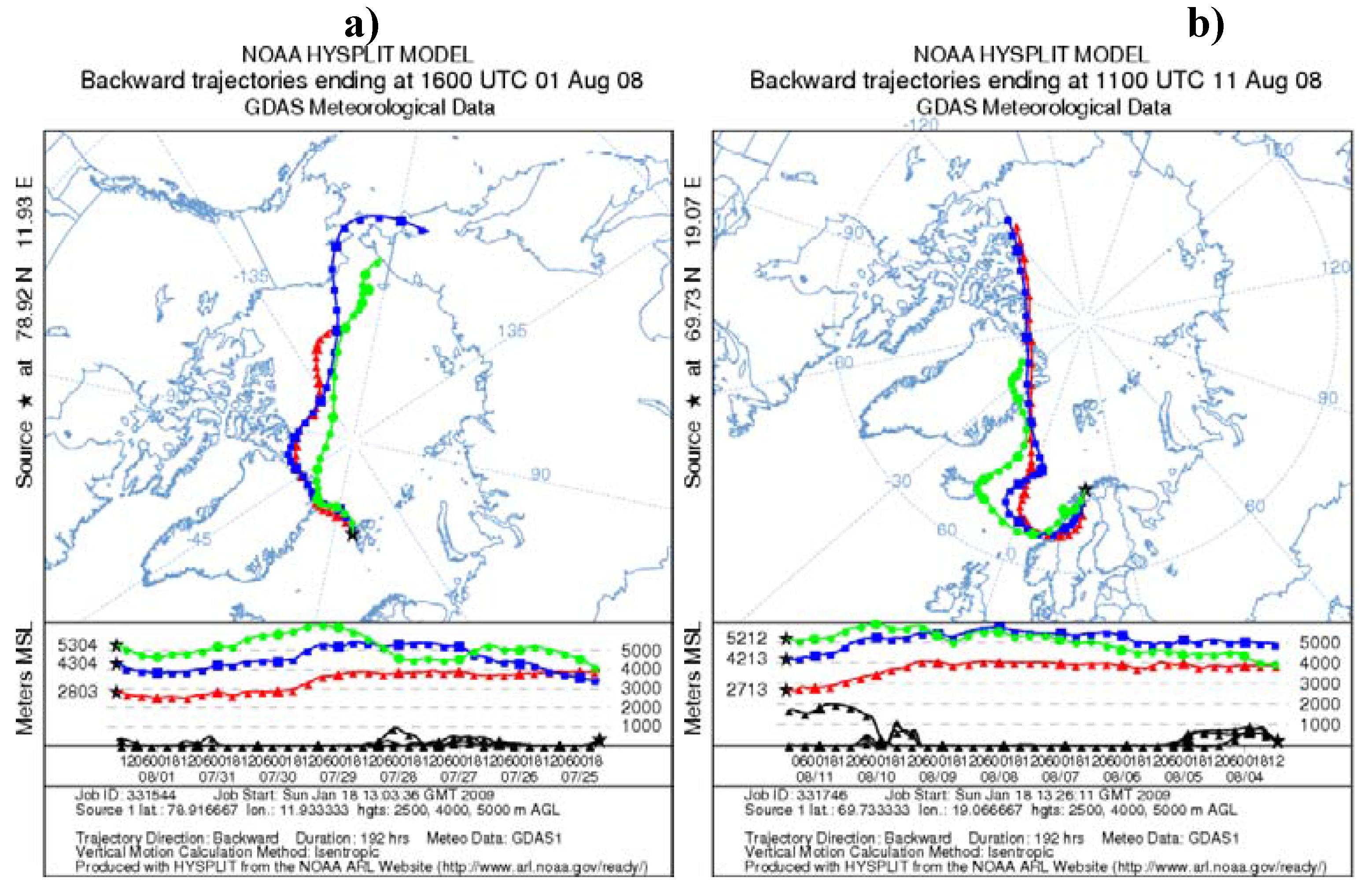
The magnitude and type of temperature and pressure advection can be manually assessed by comparing the angle between isohypses relative topography 500/1,000 hPa density and the isohypses of absolute topography (500 hPa) density.

Figure 3. Absolute geopotential layer (bold black lines) and relative topography 500/1000 layer temperature over the Finokalia station (red cross). (a) Parallel isotherms and isobars on 29 July. (b) The next 24 h movements show the dynamic changes crossing isotherms and isobars during advection on 30 July. (c) After the advection episode and during the highest values of AOD. (d) After advection episode and decreasing values of AOD.

Figure 3. Absolute geopotential layer (bold black lines) and relative topography 500/1000 layer temperature over the Finokalia station (red cross). (a) Parallel isotherms and isobars on 29 July. (b) The next 24 h movements show the dynamic changes crossing isotherms and isobars during advection on 30 July. (c) After the advection episode and during the highest values of AOD. (d) After advection episode and decreasing values of AOD.

Figure 3 shows the changes during the cold and warm advection episodes from 29 July to 2 August. During the first part of the episode, (a) figure, the significant changes in movements of pressure surface upward from the south of Finokalia station was observed. The surrounding heating/cooling rate over the station was estimated at around −2 K/h. During next 24 hours, in this case, the cooling rate decreased to −1 K/h (this is not shown) with the dynamic changes of height of the 584 gpdm isohypses.

This has been assumed as a warm advection. The episode of cold advection appeared during the crossing isotherms and isohypses on 30 July, (b) figure. After this episode the 584 gpdm isohypses was positioned south of Finokalia station and this was the tendency for a longer period of time (several hours). The heating rate of the layer increased to 0.5 K/h over a very short period of time (in about 6 hours), Figure (d).

During these days with increasing western air intrusions the attenuation caused by aerosol scattering was lowest at heights up to 5 km (29 July). Simultaneously it was highest at the altitude in a layer to 1.5 km (Figure 4a). These three mean altitudes layers of data were reversely reflected during this measurement. For two separated days highest backscattering parameter at altitudes between 1.5 and 3 km was observed during “troughs flow” and before this event in 0.3–1.5 km layer.

Figure 4. (a) Backscatter coefficient mean values at three altitude layers during the “troughs flow” event. (b) Measured AOD at 532nm during the SOAP experiment. Values were gathered in the afternoon (16:00–17:30).

Figure 4. (a) Backscatter coefficient mean values at three altitude layers during the “troughs flow” event. (b) Measured AOD at 532nm during the SOAP experiment. Values were gathered in the afternoon (16:00–17:30).

This is illustrated by a 500 hPa surface in Figure 5. The differences in value exceeded −1.912×10⁻⁶ (msr)⁻¹ (one order of magnitude). The differences in range 3 to 5 km were smaller and exceeded 1.684 × 10⁻⁷ (msr)⁻¹. The direction of the flow at about 5.8 km a.s.l. increased the attenuation by aerosols at altitudes between 1.5 to 3 km and simultaneously decreased it at altitudes up to 5 km. It clearly indicates the Mediterranean-wards air direction. The significant order of topographic isobars (white contours with geopotencial height units [gp in decameters]) represents the surfaces of ridges (that can be identified as regions where the height contours are deflected into the northern direction and the ridges aloft are associated with heights at the surface) and troughs (that can be identify as regions where the height contours are deflected in to the south direction. The Troughs aloft associated with Lows at the surface. The aerosol optical depth measured during the SOAP experiment show (Figure 3b) the relation between the northern mid-troposphere flow over the Finokalia station and its influence on aerosol variation. The main change came from the boundary layer with no pointed direction, but the source region of main circulation can be pointed by using the baric topography charts.

Figure 5. The through event on 31 July 2006 at 12 UTC at 500 hPa pressure surface (black lines) with temperature at these surfaces (colored scale) over the Finokalia station on Crete (marked as green cross). The arrow marks approximated direction of the advection.

Figure 5. The through event on 31 July 2006 at 12 UTC at 500 hPa pressure surface (black lines) with temperature at these surfaces (colored scale) over the Finokalia station on Crete (marked as green cross). The arrow marks approximated direction of the advection.

Our observations confirm that the differential temperature advection enhances the upper level height anomalies in developing disturbances. Below the 500 hPa ridge there is a strong warm advection associated with the warm front whereas below 500 hPa trough there is a strong cold advection associated with the cold front [41]. The relation between the AOD and the advection of air mass can be also analyzed by the relative topography charts. Implementation of this manual analysis of upper air charts to further works gave us similar results at higher latitudes.

4.2. Arctic Region

The data gathered during the scientific cruise of r/v Oceania to the Arctic region in 2008 allows for the comparison of aerosol optical depth characteristics in coastal and pure marine environments.

Figure 6 shows the ridges of developing surfaces under which the measurements of aerosol optical depth were possible. For 24 and 27 July increasing number of coarse particles and simultaneously decreasing number of fine mode particles can be observed (Figure 8). At the same time analyses of relative topography show, that on 24 July there was no advection and the west coast of Spitsbergen was under the 0 K/h influence.

Figure 6. (a), (b) North hemisphere projection for 500 hPa charts with arrows marking the approximated direction of the ridge surfaces over the marine environment (red cross). (c),(d) Absolute geopotential layer (bold black lines) and relative topography 500/1000 layer temperature over Spitsbergen (red cross) on 27 July 2008.

Figure 6. (a), (b) North hemisphere projection for 500 hPa charts with arrows marking the approximated direction of the ridge surfaces over the marine environment (red cross). (c),(d) Absolute geopotential layer (bold black lines) and relative topography 500/1000 layer temperature over Spitsbergen (red cross) on 27 July 2008.

The trajectory of the most “extreme” differences between the air mass directory at upper troposphere are shown in Figure 9. The flows from the North Pole stabilize the values of AOD but with recognizable variations in the AOD values. At the same time above the sea level the conditions present the agreement with 500 hPa surface charts. This may suggest the developing and stable pressure centers up to a middle troposphere. The lowest values of AOD were observed during high systems of pressures at sea level with simultaneous ridge surfaces at 500 hPa (Figure 7). The fine mode aerosols were detected (Figure 8), which confirms the pure Greenland air flow (Figure 7 and Figure 9a).

Figure 7. (a), (b), Northern hemisphere 500 hPa charts with an arrows marks the approximated direction of the ridge surfaces over the marine environment (00 UTC and 12 respectively). (c), (d) Sea Level Pressure (SLP) charts with visible agreement with baric surface charts. The example with one of the lowest AOD values in the Spitsbergen region (red cross) in 2008 (00 UTC and 12 respectively).

Figure 7. (a), (b), Northern hemisphere 500 hPa charts with an arrows marks the approximated direction of the ridge surfaces over the marine environment (00 UTC and 12 respectively). (c), (d) Sea Level Pressure (SLP) charts with visible agreement with baric surface charts. The example with one of the lowest AOD values in the Spitsbergen region (red cross) in 2008 (00 UTC and 12 respectively).

On 27 July the situation changed dynamically and the conditions appeared with more dense isobars and isotherms which contributed to high gradient between the variables (Figure 6c,d). Aerosol optical depth and the Ångström parameter over the macro-meteorological conditions from Figure 7 are shown in Figure 8. The range of the size of aerosols can be interpreted according to Ångström formula. With increasing values between the higher and lower wavelength, the exponent became higher, and with decreasing values between the higher and lower wavelength the exponent became lower. This suggests the coarse mode particles dominating in the size distribution. According to this rule it was possible to asses the size of aerosols.

Figure 8. Aerosol optical depth values derived from the Microtops II sunphotometers with calculated Ångström parameter during the r/v Oceania cruise in Spitsbergen region in 2008.

Figure 8. Aerosol optical depth values derived from the Microtops II sunphotometers with calculated Ångström parameter during the r/v Oceania cruise in Spitsbergen region in 2008.

The fine particles were observed on 24 July (Figure 8) when the measurement region was under the developing ridge structure with source region pointed at North Sea. This process evolved into the deep ridge structure where the aerosols became bigger (27 July). The source region was southern Norway.

Relatively high AOD values with coarse aerosol particles was observed at the fiord region which was under shallow through baric surface (10 August) with the centre over the North Pole. The analysis of backtrajectories indicates northern flow impact on the measurement region.

One day later the source region can be pointed at more southerly (Figure 9b), where the coarse particles were observed (Figure 8). Also the one of the lowest AOD values was observed under the ridge baric surface (1 August; Figure 7 and Figure 8). The source region was mostly northerly as shown in Figure 9. To obtain more detailed view of changes and summarize the experiment the mean spectral characteristics of AOD are presented in Figure 10 below.

One more approach of upper troposphere charts in manual analysis was applied to present using the data obtained during the MACRON campaign in summer 2007 on Andoya Island in northern Norway. The main field of analysis was focused on northern hemisphere jet stream charts available from San Francisco State University (http://squall.sfsu.edu/crws/archive/jetstream_archive.html).

Figure 9. NOAA HYSPLIT backward isentropic trajectories (a) during the one of the lowest mean AOD events with northern flows. (b) the day with one of the highest mean AOD with coastal southern flow. Source pointed at different locations came from the track of cruise.

Figure 9. NOAA HYSPLIT backward isentropic trajectories (a) during the one of the lowest mean AOD events with northern flows. (b) the day with one of the highest mean AOD with coastal southern flow. Source pointed at different locations came from the track of cruise.

Figure 10. Mean spectral characteristics during r/v Oceania cruise in Spitsbergen region (2008).

Figure 10. Mean spectral characteristics during r/v Oceania cruise in Spitsbergen region (2008).

An analysis of each 6 hour chart was done to detect the significant changes on 300 mb baric surfaces. During 27 - 31 July period the Jet Stream trajectory was situated beyond the measurement station, over the Western Europe. The position of the Jet Stream was changed counterclockwise, with high wind speed of about 148 km/h on 300 hPa charts. It was the “first front” of turbulence during which, the curves of the Jet Stream did not reach the high latitudes over the Lofoten Islands and the aerosol optical parameters were affected from southern direction which was verified with the METAR information for ENAN (01010) at Andoya airport, with about 5.5 km distance from the measurement points (data from Weather Underground service). The aerosol optical depth and wind conditions are shown in Figure 11 a) and Figure 11b).

Figure 11. (a) Aerosol Optical Depth (derived from the Microtops II) and wind speed. (b) Wind speed and wind direction during the MACRON experiment. Meteorological data were taken from METAR Information for ENAN (01010) in Andoya, Norway.

Figure 11. (a) Aerosol Optical Depth (derived from the Microtops II) and wind speed. (b) Wind speed and wind direction during the MACRON experiment. Meteorological data were taken from METAR Information for ENAN (01010) in Andoya, Norway.

The second “front” of event was found during 7 - 8 August and it was the maximum of enhancement in the AOD measurements. The direction of wind flows changed from S to NE on 7 August and the same episode repeated on the 8 August (Figure 12 a,b). The wind speed during the episodes was not very high, but the significant changes of this parameter appeared at the Andoya airport one day later.

The spectral mean behavior of AOD from MACRON campaign (Figure 13) shows the basic changes in atmospheric column in some optical ways. It can by explained using the upper air charts by interpreting the density of isobars, direction of advection and the temperature of basic pressure layers.

5. Conclusions

This paper examined the spatial and temporal variation of aerosol optical depth in different regions using the relative troposphere charts. These charts show the entire “atmospheric hypsography” from polar regions to tropic zones over the Mediterranean region. Therefore, these structures can become the common denominator of analysis tools and what is most significant, they are available from the Internet sources. Comparison of manual analysis charts with empirical data derived from a lidar and Microtops II sunphotometers, allows for the detection of different behavior of aerosol optical depth under through and ridges over such different areas as the Arctic and the Mediterranean.

During this investigation the measurement of useful backscatter coefficient parameter was made at an altitude of above 1.5 km and it occurred that the columnar AOD can be significantly affected by the ridges and troughs of northern hemisphere circulation. During 31 July 2006 over Finokalia station, the through flow event, we could observe backscatter coefficient once with maximum values up to 3 km a.s.l. and at the same time minimum of these values from 3 to 5 km a.s.l. during all measurements days.

Figure 12. (a) Absolute geopotential layer (bold black lines) and relative topography 500/1000 layer temperature. (b) Jet stream event during measurements. Data during the jet stream event over Andoya Island (red cross) with approximated direction of air mass direction (arrow).

Figure 12. (a) Absolute geopotential layer (bold black lines) and relative topography 500/1000 layer temperature. (b) Jet stream event during measurements. Data during the jet stream event over Andoya Island (red cross) with approximated direction of air mass direction (arrow).

Figure 13. Mean spectral characteristics of aerosol optical depth before, during and after the Jet Stream event during the MACRON experiment on Andoya Island.

Figure 13. Mean spectral characteristics of aerosol optical depth before, during and after the Jet Stream event during the MACRON experiment on Andoya Island.

It was possible to observe this sources flow dynamic by using these parallel thematic surfaces of the atmosphere called relative topography charts. By using this thematic “dividing” we could point out the source region of aerosols in the upper air layer and in the same way point to the boundary layer in which the changes can be reflected with some delay. The opposite dynamic, which was significant and immediately was shown in Lofoten Islands example during MACRON experiment. The range of changes of the AOD between the “Before” and “During” Jet Stream event state was quite spectacular with differences of 0.15 for 380 nm and 0.05 for 675 nm.

The comparison of experimental results provides the following conclusions regarding the range of influence of baric structures on AOD values.

In the Arctic region (MACRON, AREX experiments):

• affected by developing structures reaching the nearest region in synoptic scale
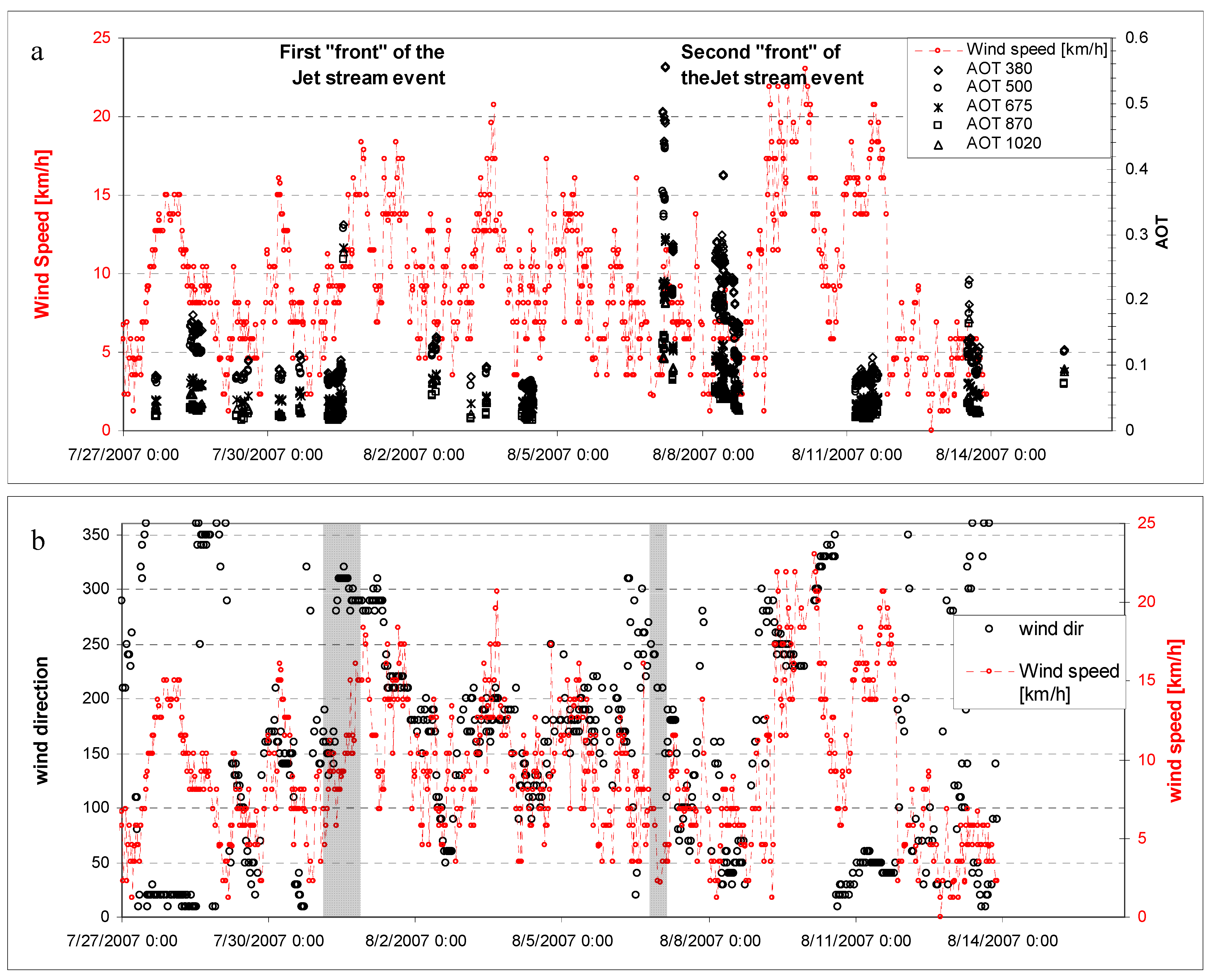
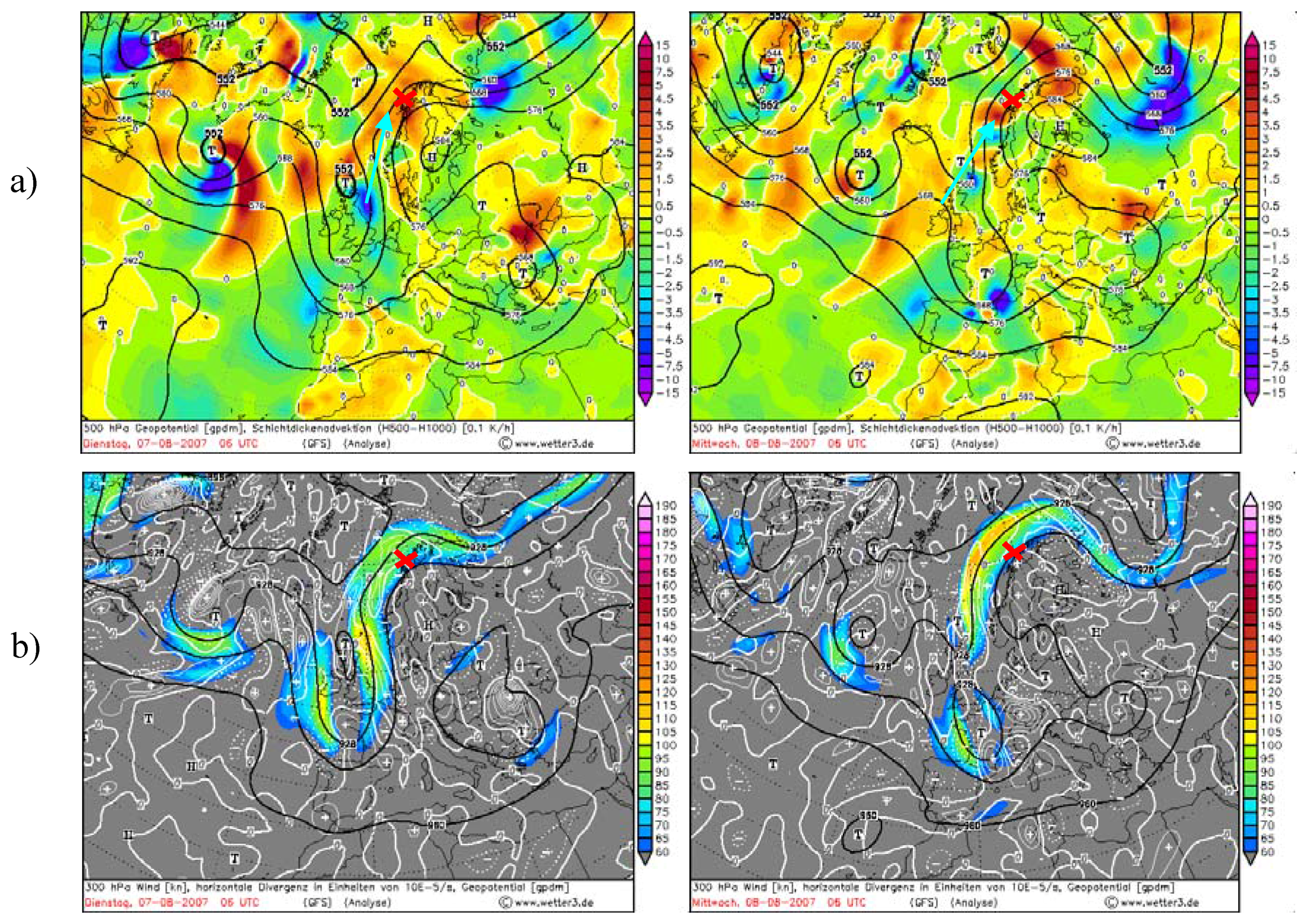
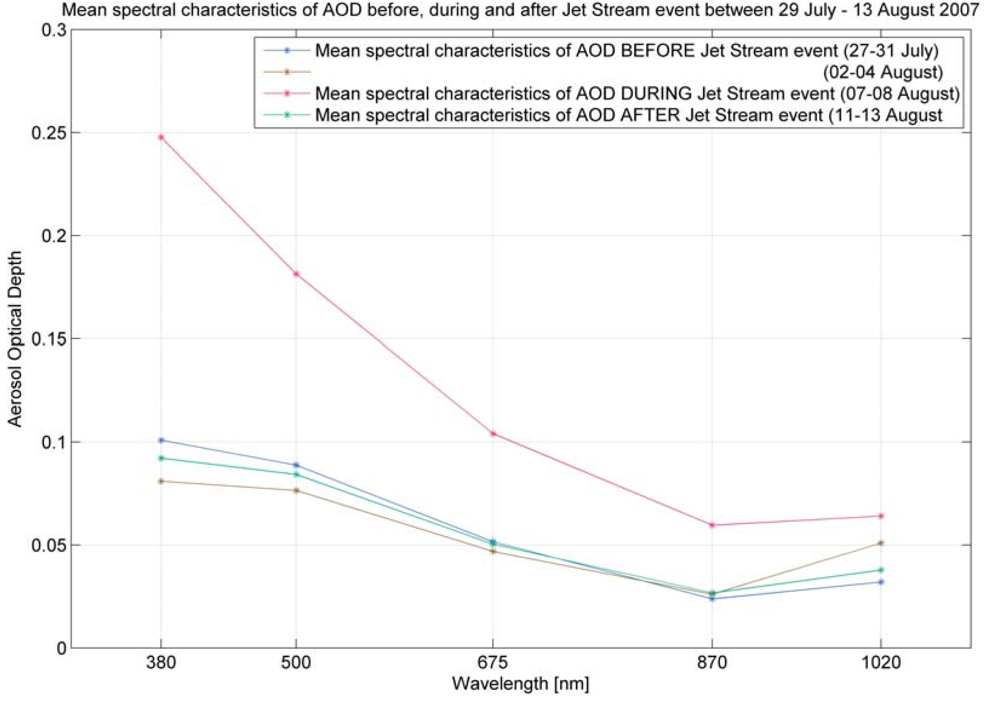
• under the Jet Stream as an extended baric structure causing Sahara dust flow to the North in the Mediterranean region (SOAP experiment):
• affected by developed structures (trough) reaching from far North to Crete
• under shallow baric structures directed over the Mediterranean Sea

References

1. Shahgedanova, M.; Lamakin, M. Trend in aerosol optical depth in the Russian Arctic and their links with synoptic climatology. Sci. Total Envir. 2005, 41, 3–148. [Google Scholar] [CrossRef] [PubMed]
2. Smirnov, A.; O’Neill, N.T.; Royer, A.; Tarussov, A. Aerosol optical depth over Canada and the link with synoptic air mass types. J. Geophys. Res. 1996, 101, 299–318. [Google Scholar] [CrossRef]
3. Dayan, U.; Lamb, D. Global and synoptic-scale weather patterns controlling wet atmospheric deposition over central Europe. Atmos. Environ. 2005, 39, 521–533. [Google Scholar] [CrossRef]
4. Zielinski, T.; Zielinski, A. Aerosol extinction and optical thickness in the atmosphere over the Baltic Sea determined with lidar. J. Aerosol Sci. 2002, 33, 47–61. [Google Scholar] [CrossRef]
5. Zielinski, T. Changes in aerosol concentration with altitude in the marine boundary layer in coastal areas of the southern Baltic Sea. Bull. PAN Earth Sci. 1998, 46, 133–139. [Google Scholar]
6. Piazzola, J.; Bouchara, F.; de Leeuw, G.; Van Eijk, A.M.J. Development of the Mediterranean extinction code (MEDEX). Opt. Eng. 2003, 42, 912–924. [Google Scholar] [CrossRef]
7. Villevalde, Y.V.; Yakovlev, V.V.; Smyshlayev, S.P. Measurements of atmospheric optical parameters in the Baltic Sea and Atlantic Ocean. In Studies of the southern part of the Norwegian Sea; Kluikov, Y.Y., Ed.; Gidrometeoizadat: Moscov, Russia, 1989; pp. 105–110. [Google Scholar]
8. Kuśmierczyk-Michulec, J.; Darecki, M. The aerosol optical thickness over the Baltic Sea. Oceanologia 1996, 38, 423–435. [Google Scholar]
9. Zielinski, T. Physical properties of aerosol near-water layer in coastal areas. Rozprawy i Monografie IOPAN 2006, 18, 164. [Google Scholar]
10. Mauger, G.S. Synoptic sensitivities of subtropical clouds separating aerosol effects from meteorology . PhD Dissertation in Oceanography, University of California, San Diego, USA, 2008. [Google Scholar]
11. Zhang, T.; Scambos, T.; Haran, T.; Hinzman, L.D.; Barry, R.G.; Kane, D.L. Ground-based and satellite-derived measurements of surface albedo on the North slope of Alaska. J. Hydrometeorology 2003, 4, 77–91. [Google Scholar] [CrossRef]
12. Dubovik, O.; Holben, B.; Eck, T.; Smirnov, A.; Kaufman, Y.; King, M.; Tanre, D.; Slutsker, L. Variability of absorption and optical properties of key aerosol types observed in worldwide locations. J. Atmos. Sci. 2002, 59, 590–608. [Google Scholar] [CrossRef]
13. Smirnov, A.; Holben, B.N.; Sakerin, S.M.; Kabanov, D.M.; Slutsker, I.; Chin, M.; Diehl, T.L.; Remer, L.A.; Kahn, R.; Ignatov, A.; Liu, L.; Mishchenko, M.; Eck, T.F.; Kuscera, T.L.; Giles, D.; Kopelevich, O.V. Ship-based aerosol optical depth measurements in the Atlantic Ocean: Comparison with satellite retrievals and GOCART model. Geophys. Res. Lett. 2006, 33, L14817. [Google Scholar] [CrossRef]
14. Remiszewska, J.; Flatau, P.J.; Markowicz, K.M.; Reid, E.A.; Reid, J.S.; Witek, M.L. Modulation of the aerosol absorption and single-scattering albedo due to synoptic scale and sea breeze circulations: United Arab Emirates experiment perspective. J. Geophys. Res. 2007, 112, D05204. [Google Scholar] [CrossRef]
15. Deshpande, C.G.; Kamra, A.K. Aerosol size distributions in the north and south Indian ocean during the northeast monsoon season. Atmos. Res. 2002, 65, 51–76. [Google Scholar] [CrossRef]
16. Smirnov, A.; Villevalde, Y.; O’Neill, N.T.; Royer, A.; Tarussov, A. Aerosol optical depth over the oceans: analysis in terms of synoptic air mass types. J. Geophys. Res. 1995, 100 (D8), 16639–16650. [Google Scholar] [CrossRef]
17. Mulcahy, J.P.; O’Dowd, C.D.; Jennings, S.G.; Ceburnis, D. Significant enhancement of aerosol optical depth in marine air under high wind conditions. Geophys. Res. Lett. 2008, 35, L16810. [Google Scholar] [CrossRef]
18. Jensen, D.; Gathman, S.; Zeisse, C.; Littfin, K. EOPACE (Electrooptical Propagation Assessment in Coastal Environments) overview and initial accomplishments. J. Aerosol Sci. 1999, 30, S53–S54. [Google Scholar] [CrossRef]
19. Jensen, D.; Zeisse, C.; Littfin, K.; Gathman, S. EOPACE (Electrooptical Propagation Assessment in Coastal Environments) overview and initial accomplishments. In Propagation and Imaging Through the Atmosphere; Bissonnette, L.R., Dainty, C., Eds.; SPIE-International Society for Optical Engineering: Washington, DC, USA, 1997; pp. 98–108. [Google Scholar]
20. Moorthy, K.K.; Satheesh, S.K.; Murthy, B.V. Investigations of marine aerosols over the tropical Indian Ocean. J. Geophys. Res. 1997, 102 (Dl 5), 18827–18842. [Google Scholar] [CrossRef]
21. Moorthy, K.K.; Satheesh, S.K; Murthy, B.V. Characteristics of spectral optical depths and size distributions of aerosols over tropical oceanic regions. J. Atmos. Sol. Terr. Phys. 1998, 60, 981–992. [Google Scholar] [CrossRef]
22. Dion, D. On the prediction of IR aerosol extinction near the sea surface. J. Aerosol Sci. 1999, 30, S61–S62. [Google Scholar] [CrossRef]
23. Fredrickson, P.; Davidson, K. Measurement and modelling of near-ocean surface properties affecting aerosol concentration profiles during EOPACE. J. Aerosol Sci. 1999, 30, S55–S56. [Google Scholar] [CrossRef]
24. Kuśmierczyk-Michulec, J.; Rozwadowska, A. Seasonal changes of the aerosol optical thickness for the atmosphere over the Baltic Sea-preliminary results. Oceanologia 1999, 41, 127–145. [Google Scholar]
25. Li, F.; Okada, K. Diffusion and modification of marine aerosol particles over the coastal areas in China: A case study using a single particle analysis. J. Atmos. Sci. 1999, 56, 241–248. [Google Scholar] [CrossRef]
26. Tsai, Y.I.; Cheng, M.T. Visibility and aerosol chemical compositions near the coastal area in Central Taiwan. Sci. Total Environ. 1999, 231, 37–51. [Google Scholar] [CrossRef]
27. Porter, J.N.; Lienert, B.; Sharma, S.K. Using horizontal and slant lidar measurements to obtain calibrated aerosol scattering coefficients from a coastal lidar in Hawaii. J. Atmos. Oceanic Technol. 2000, 17, 1445–1454. [Google Scholar] [CrossRef]
28. Gao, Y.; Anderson, J.R. Characteristics of Chinese aerosols determined by individual-particle analysis. J. Geophys. Res. 2001, 106 (D16), 18037–18045. [Google Scholar] [CrossRef]
29. Welton, E.J.; Voss, K.J.; Quinn, P.K.; Flatau, P.J.; Markowicz, K.; Campbell, J.R.; Spinhirne, J.D.; Gordon, H.R.; Johnson, J.E. Measurements of aerosol vertical profiles and optical properties during INDOEX 1999 using micropulse lidars. J. Geophys. Res. Atmos. 2002, 107 (D19), 8019. [Google Scholar] [CrossRef]
30. Karasinski, G.; Kardas, A.E.; Markowicz, K.; Malinowski, S.P.; Stacewicz, T.; Stelmaszczyk, K.; Chudzynski, S.; Skubiszak, W.; Posyniak, M.; Jagodnicka, A.K.; Hochhertz, C.; Woeste, L. LIDAR investigation of properties of atmospheric aerosol. Eur. Phys. J. 2007, 144, 129–138. [Google Scholar] [CrossRef]
31. Markowicz, K.M.; Flatau, P.J.; Kardas, A.E.; Remiszewska, J.; Stelmaszczyk, K.; Woeste, L. Ceilometer retrieval of the boundary layer vertical aerosol extinction structure. J. Atmos. Oceanic Technol. 2008, 25, 928–944. [Google Scholar] [CrossRef]
32. Zielinski, T.; Pflug, B. Lidar-based studies of aerosol optical properties over coastal areas. Sensors 2007, 7, 3347–3365. [Google Scholar] [CrossRef]
33. Sakerin, S.M.; Kabanov, D.M. Spectral dependences of the atmospheric aerosol optical depth in the extended spectral region of 0.4-4 μm. In Sixteenth ARM Science Team Meeting Proceedings, Albuquerque, NM, USA, March 27 - 31, 2006; 2006. [Google Scholar]
34. Kabanov, D.M.; Makienko, E.V.; Rakhimov, R.F.; Sakerin, S.M. Typical and anomaly spectral behavior of aerosol optical thickness of the atmosphere in western siberia. In Tenth ARM Science Team Meeting Proceedings, San Antonio, Texas, USA, March 13-17, 2000.
35. Toledano, C.; Wiegner, M.; Garhammer, M.; Seefeldner, M.; Gasteiger, J.; Müller, D.; Koepke, P. Spectral aerosol optical depth characterization of desert dust during SAMUM 2006. Tellus Ser. B 2009, 61, 216–228. [Google Scholar] [CrossRef]
36. McCartney, J. Optics of the Atmosphere; John Wiley and Sons: New York, NY, USA, 1976. [Google Scholar]
37. Liou, K.N. An Introduction to Atmospherics Radiation; Academic Press: London, UK, 2002. [Google Scholar]
38. WMO Background Air Pollution MONitoring (BAPMON) Network Information Manual, TD-9789, September, 1990, Iqbal, Muhammad. In An Introduction to Solar Radiation; Academic Press: Toronto, Canada, 1983.
39. Georgoussis, G.; Chourdakis, G.; Landulfo, E.; Hondidiadis, K.; Ikonomou, A. Monitoring of air pollution and atmospheric parameters using a mobile backscatter lidar system. 3rd-Workshop LIDAR Measurements in Latin América. Ópt. Pura Aplic. 2006, 39, 37. [Google Scholar]
40. Walter, J.S. Principles of Meteorological Analysis; Courier Dover Publications: Phoenix, AZ, USA, 2003; p. 202. [Google Scholar]
41. Holton, J.R. An Introduction to Dynamic Meteorology, 4th ed; Academic Press: New York, NY, USA, 2004; p. 158. [Google Scholar]