1. Introduction
Over the last two decades there has been a revolution in our ability to map and monitor large areas of subaerial topography using technologies such as radar and near-infrared Light Detection and Ranging (LIDAR). Indeed, a future seems near in which high resolution topographic data will be available for all land areas on the planet. However, commensurate progress in bathymetry has not occurred and water remains a difficult medium through which to make remote measurements of topography.
Traditional field wading surveys, using GPS, total station, or leveling instruments, remain the standard for stream mapping. While such surveys can be highly accurate, these field techniques require legal access to a channel and flow conditions that allow wading. Field surveys are also slow, labor intensive, costly and often done with point measurements spaced more than 1 m apart in at least one dimension, producing DEMs with fairly coarse spatial resolution. As each point elevation measurement requires on the order of 0.5–1 minute, field surveys of even small streams are seldom attempted for channel domains longer than a few hundred meters.
Some recent progress has been made using remote passive optical systems that relate reflected solar radiation to the depth of water [
1,
2,
3,
4]. However, this technique must account for spatiotemporal changes in other variables such as substrate reflectivity due to variations in sediment type and patchy periphyton growth, water turbidity, atmospheric transmission of electromagnetic energy, and reflectance and shadowing from overhanging vegetation on stream banks. Boat-based acoustic sounding and mapping systems with GPS-derived geolocation capability can produce high quality bathymetry, but require access, navigable water, and considerable time and effort for data acquisition over large areas of channel [
5].
Water heavily absorbs the near-infrared energy of terrestrial LIDARs, making them ineffective over streams. Consequently, bathymetric LIDARs must operate in the blue–green regions of the spectrum and traditionally these systems have been designed for maximum water penetration using a relatively high-power, pulsed green laser fired at fairly low repetition rates [
6]. To maintain eye-safety during operation, each transmitted beam is dispersed to a diameter of a few meters at the water surface. Further expansion of the beam occurs across the air-water interface and in the water column, with the final beam diameter at the bottom of the water reaching up to 5 m (depth dependent) [
6]. These characteristics are advantageous in some marine applications, but cause poor resolution of the small topographic features and abrupt changes in topography typically seen in the beds and banks of rivers. In many streams, flow depths are less than 10 m and if water clarity is high, laser energy penetration to the channel bed is less problematic than achieving high spatial resolution of morphology.
In contrast to other bathymetric LIDARs, the Experimental Advanced Airborne Research LIDAR (EAARL) was designed with a lower power green laser, operated at higher pulse repetition rates with a smaller beam divergence [
7,
8]. The EAARL was first deployed in 2001 and used primarily in shallow marine and coastal environments [
7]. However, its design also is favorable for mapping the morphology of clear-water streams and in recent years the EAARL has been tested in several fluvial environments [
9,
10,
11,
12,
13]. Here we describe the basic characteristics of the EAARL system including data acquisition and processing. We assess the data quality and discuss applications for mapping, managing and monitoring streams and riparian habitat and modeling water flow and sediment transport. We also illustrate a method of frequency domain analyses of these continuous data and introduce a GIS-based tool to automatically measure channel geometry in cross sections and long profiles extracted from any high-resolution channel DEM.
2. Experimental Advanced Airborne Research LIDAR (EAARL)
2.1. Technical Characteristics
The EAARL is an aquatic-terrestrial LIDAR capable of high-resolution cross-environment surveys of shallow bathymetry, subaerial bare earth topography and vegetation three-dimensional structure in one integrated mission.
Table 1 summarizes the system technical specifications and further technical descriptions have been published elsewhere [
7,
8,
14,
15]. The core of the sensor is a low power, narrow-beam, full waveform, raster scanning green laser with a short pulse length. The low power of the laser allows it to be operated with a small beam divergence that keeps the energy tightly focused in a footprint with a diameter of only 15–20 cm while maintaining eye safety when flown from the nominal operating altitude. The pulse frequency of the EAARL is high, relative to other bathymetric LIDARs, and automatically varied along each raster scan to produce a constant 2 m spacing of measurements in the cross track direction. This combination of design elements allows high spatial resolution of morphologic features, including areas with sharp topographic curvature, such as channel bedforms and the edges of stream banks. The narrow beam and short pulse length also improve resolution of the water surface and bottom reflections by reducing pulse stretching from scattered photons at those interfaces and in the water column.
Table 1.
EAARL Technical Specifications [
7,
8,
14,
15].
Table 1.
EAARL Technical Specifications [7,8,14,15].
| Total system weight | 113 kg |
| Maximum power requirement | 28 VDC at 26 amps |
| Nominal survey altitude | 300 m (AGL) |
| Nominal survey flight speed | 50 m/sec |
| Inertial navigation system | 200 Hz |
| Precision kinematic GPS | 2 Hz |
| Laser | Neodymium-doped Yttrium Aluminum Garnet (Nd:YAG) |
| Laser wavelength | 532 nm |
| Laser pulse energy | Up to 70 μJ/pulse (eye safe) |
| Laser pulse length | 1.2 nsec (full width at half-maximum) |
| Laser field-of-view | 1.5–2 mrad |
| Laser beam divergence | 0.5 mrad |
| Laser spot diameter from 300 m AGL | 20 cm |
| Laser pulse frequency | 3–10 kHz |
| Raster scan rate | 25/sec |
| Digitized waveform samples per laser pulse | 16,384 |
| Digitizer temporal resolution | 1 nsec (14.9 cm in air, 11.3 cm in water) |
| Data swath width from 300 m AGL | 240 m |
| Single pass sample spacing | 2 m cross track, 2 m average along track |
| Vertical accuracy | 10–15 cm RMSE |
| Horizontal accuracy | <1 m RMSE |
| Operation water depths | 0.2–25 m (clarity dependent) |
| Other integrated sensors | RGB digital camera (~40 cm pixel); High resolution CIR digital camera (~15 cm pixel) |
| Processing software | Airborne Laser Processing Software (ALPS) |
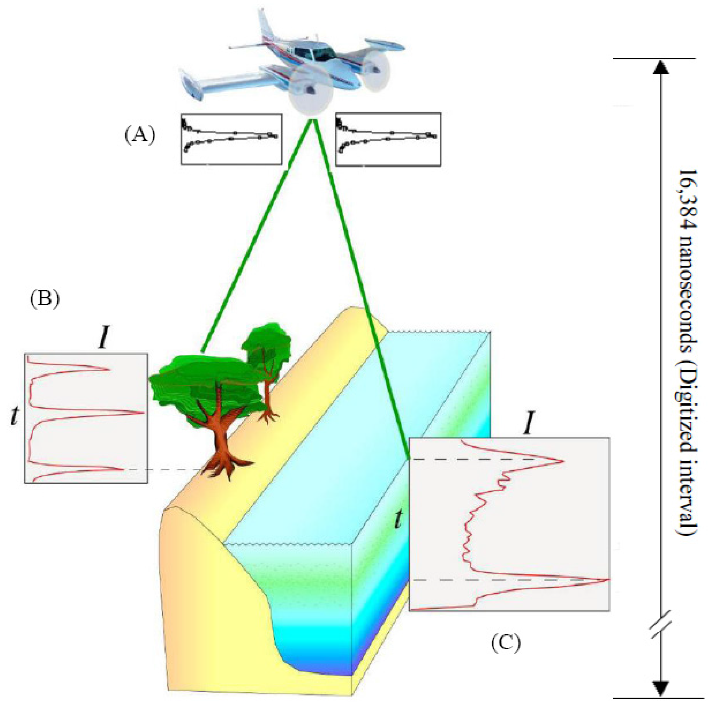
A high speed waveform digitizer, connected to a subnanosecond photo-detector, samples each pulse of outgoing laser energy to establish its shape, timing and amplitude, critical for accurate measurement of energy travel time (
Figure 1).
Figure 1.
Schematic of EAARL data acquisition [
16]. (A) Example transmitted pulses; (B) Received waveform of energy (I) as a function of time (t) reflected from vegetation; (C) Received waveform of energy reflected through water. The upper and lower peaks are reflections from the water surface and the bed, respectively.
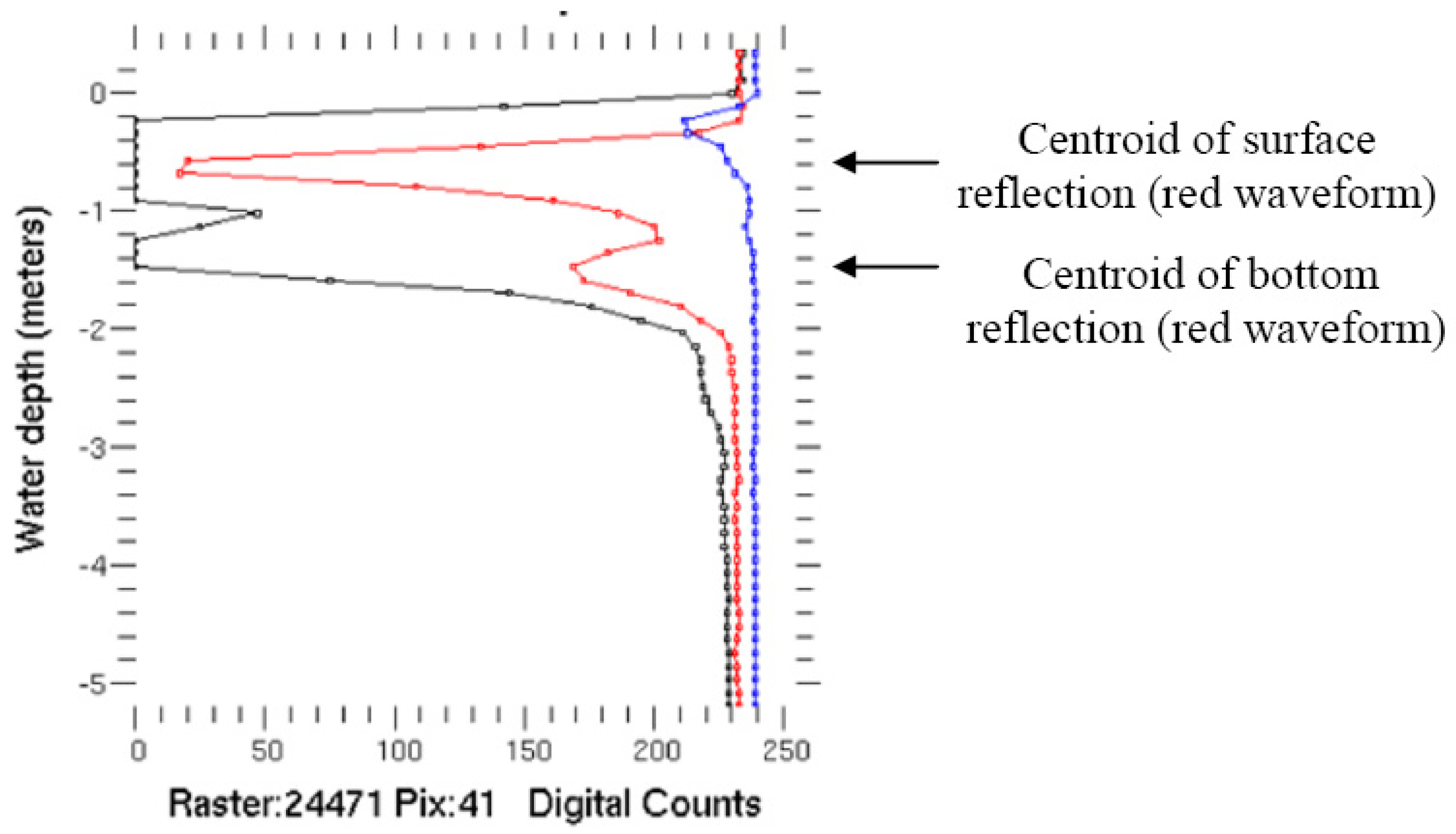
Backscattered energy from each laser pulse is received by an array of three similar digitizer-detectors, each with a temporal resolution of 1 ns (
Figure 2). The most sensitive detector (black) receives 90% of the photons, the second-most sensitive channel (red) then receives 9% and finally the least sensitive (blue) receives 1%. This hardware arrangement gives the sensor the wide dynamic range necessary to operate across the typical variety of reflection targets in fluvial environments that include features such as exposed river gravel and sand bars, subaerial vegetation, water of variable depths and clarity, diverse submerged channel bed sediment, and aquatic vegetation. For example, in
Figure 2 the most sensitive detector is saturated by a Fresnel water surface reflection and a reflection from the submerged topography. The intermediate sensitivity detector records both the surface and bottom topography reflections. The lowest sensitivity detector records the surface reflection, but barely registers the energy return from the bottom. In this case, the software would identify the intermediate detector as the best for a depth determination. The depth of the bottom reflection would be calculated as the difference between the centroids of the surface and bottom reflections: about 0.9 m. The waveforms of time-rate-of-return of energy from each pulse are analyzed in real-time by an adaptive processor that identifies and records on hard drives key features including the transmitted pulse, the first and last energy returns and other relevant portions of each waveform.
Figure 2.
Typical bathymetric waveforms for three photo-detectors with a strong water surface reflection and weaker bottom reflection. Each detector independently records the time history of energy from each laser pulse. Here the three records are also plotted independently, and thus have small offsets on the vertical axis. Normally the offsets are removed during calibration. Digital counts are inverted in the photodetector and lower counts correspond to higher energy return.
The green LIDAR is complemented by two digital cameras (one RGB and one CIR) that operate at 1 Hz with a field-of-view that covers slightly more than the nominal 240 m swath width of the LIDAR scanner. The CIR photos are georeferenced in the ALPS software to an accuracy of 1–5 m, depending on roughness of the terrain. A simple orthorectification is done using one average elevation for each image. More sophisticated and accurate georeferencing and orthorectification can be done outside the ALPS software.
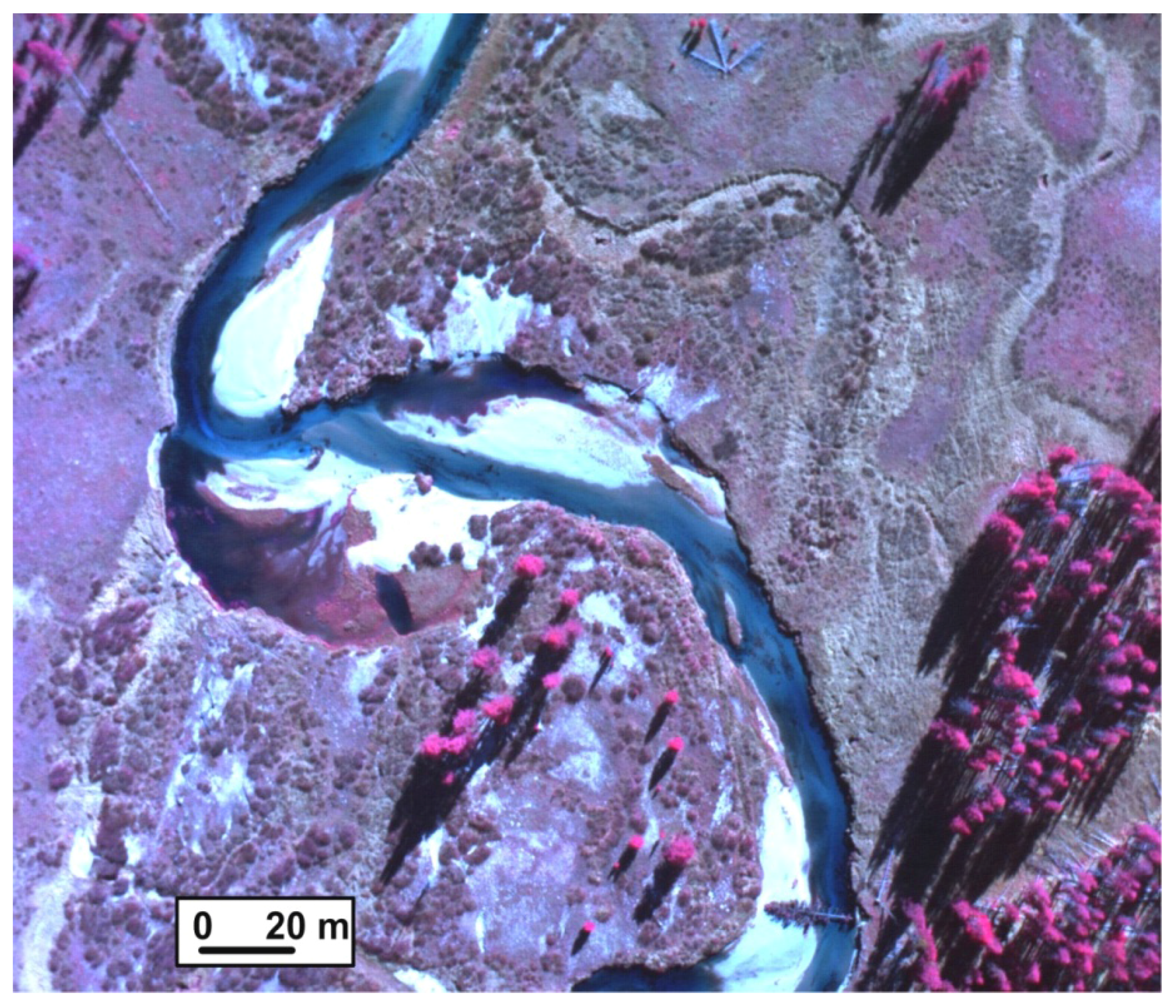
Figure 3 is an example of the high resolution CIR digital multispectral imagery.
The size, light weight and low power requirements of the instrument allow surveys in small aircraft, primarily a Cessna 310 or a Pilatus PC-6, with a 2-person crew of pilot and LIDAR operator. The turbocharged PC-6 is optimal for surveys in mountainous conditions. Each elevation measurement by the EAARL is geo-located using a combination of precision kinematic differential GPS receivers to constantly record the aircraft location and an inertial attitude measurement system to record pitch, roll and heading. Data from temporary GPS base stations in the field area are used to postprocess the aircraft GPS information if permanent base stations in close proximity are not available.
Figure 3.
CIR digital imagery from Elk Creek, tributary to the upper Middle Fork Salmon River, ID, USA. Pixel resolution is about 15 cm.
Figure 3.
CIR digital imagery from Elk Creek, tributary to the upper Middle Fork Salmon River, ID, USA. Pixel resolution is about 15 cm.
2.2. Data Processing
After the waveforms are recorded and precision GPS trajectory solutions are established to closely geo-locate the data, the user has full control over further postprocessing. This is done with the Airborne Laser Processing Software (ALPS), that is custom built open-source code developed primarily by NASA and the USGS [
16,
17]. ALPS is freely available to all EAARL collaborators and is operated on a Linux platform. The code is written in Yorick, an interpreted programming language with an array syntax optimized to rapidly handle large data sets [
18]. The graphical user interface is constructed in the open source scripting languages Tcl and Tk (
Figure 4 illustrates the major elements of this interface). ALPS interrogates each waveform to extract the range to the first, last and other significant returns with greater precision than the real-time adaptive processor. Algorithms are selected to process for either vegetation (first surface), topography under vegetation (bare earth) or bathymetry. This processing is done over areas selected from a map of flight tracks and is conducted in either interactive or batch mode, the latter automatically generates topography data in 2 km by 2 km tiles. Using a high-end PC, data covering a single tile can be processed in about 15 minutes.
Random consensus (RCF) and iterative random consensus (IRCF) filters are available to remove false bottom returns from bathymetry data and vegetation returns during processing for bare earth data [
6,
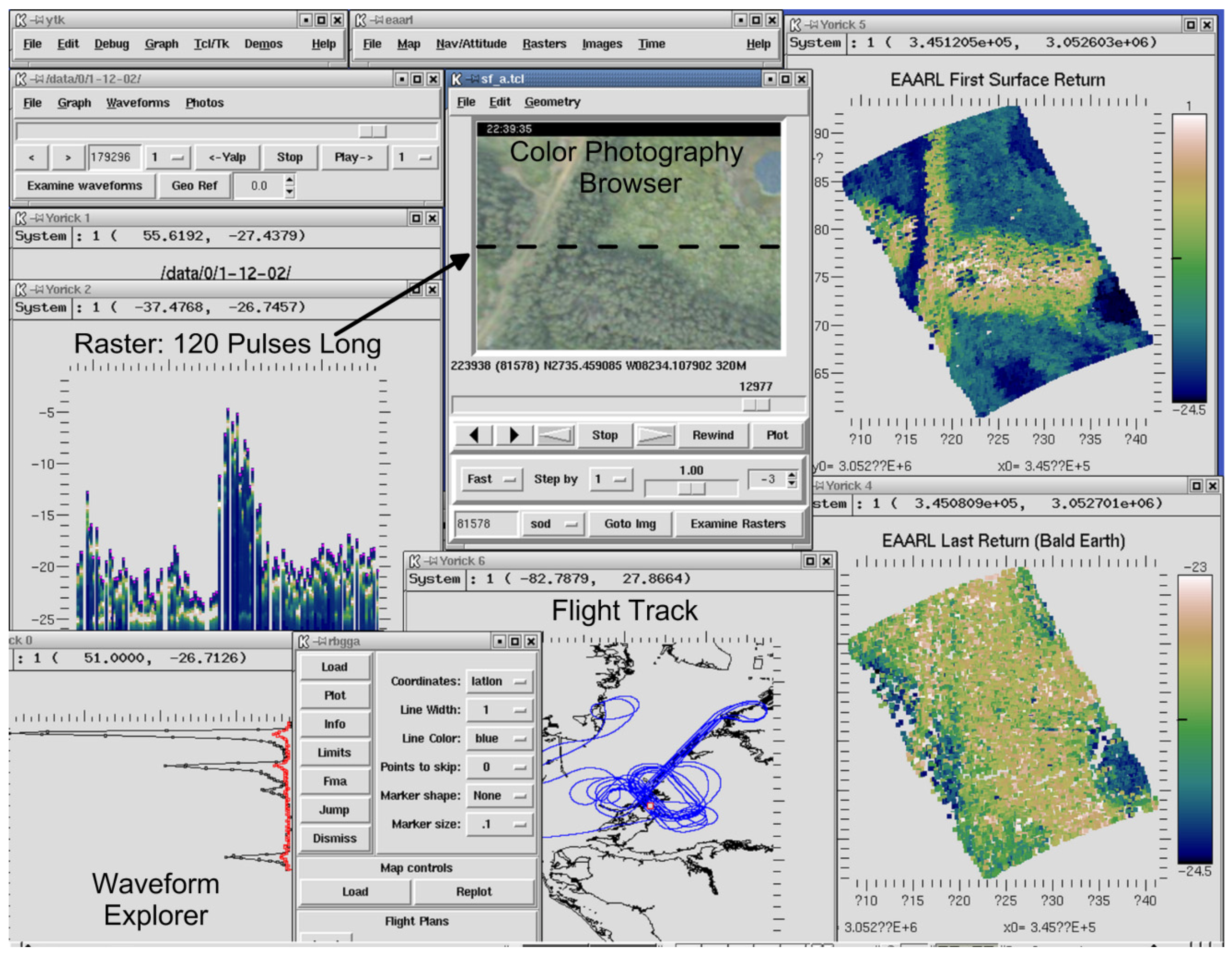
19]. Further manual editing is often necessary to remove remaining vegetation or other extraneous points. A particular issue is vegetation on stream banks, as automated filters have difficulty differentiating the bare earth surface of a steep bank from low vegetation. Manual editing of data may require several days to weeks, depending on the length and complexity of the channel and the characteristics of the riparian vegetation. Data are processed in the WGS84 datum, but can be converted into any of several other datums, and ellipsoidal heights are converted to orthometric heights (NAD83 to NAVD88) using a geoid model. Individual waveforms can be selected from sites in the displayed data for further investigation of their characteristics. Single rasters, 120 laser pulses long, can also be viewed. Before gridding into DEMs the data are converted to a .xyz or .las file format. A variety of gridding options are provided to generate elevation rasters within ALPS or the filtered data clouds can be exported to other software for this purpose. The RGB and CIR images can be played sequentially in a viewer and are dynamically linked to the flight track map. Using this feature either an image can be selected that corresponds to a location chosen on the map, or the location of any image chosen in the playback viewer can be found on the flight track map.
Figure 4.
Airborne LIDAR Processing Software (ALPS) user interface. All inset windows display information from the position of the red dot in the lower middle of the flight track map.
Figure 4.
Airborne LIDAR Processing Software (ALPS) user interface. All inset windows display information from the position of the red dot in the lower middle of the flight track map.
3. EAARL System Performance
To illustrate the capabilities of this instrument,
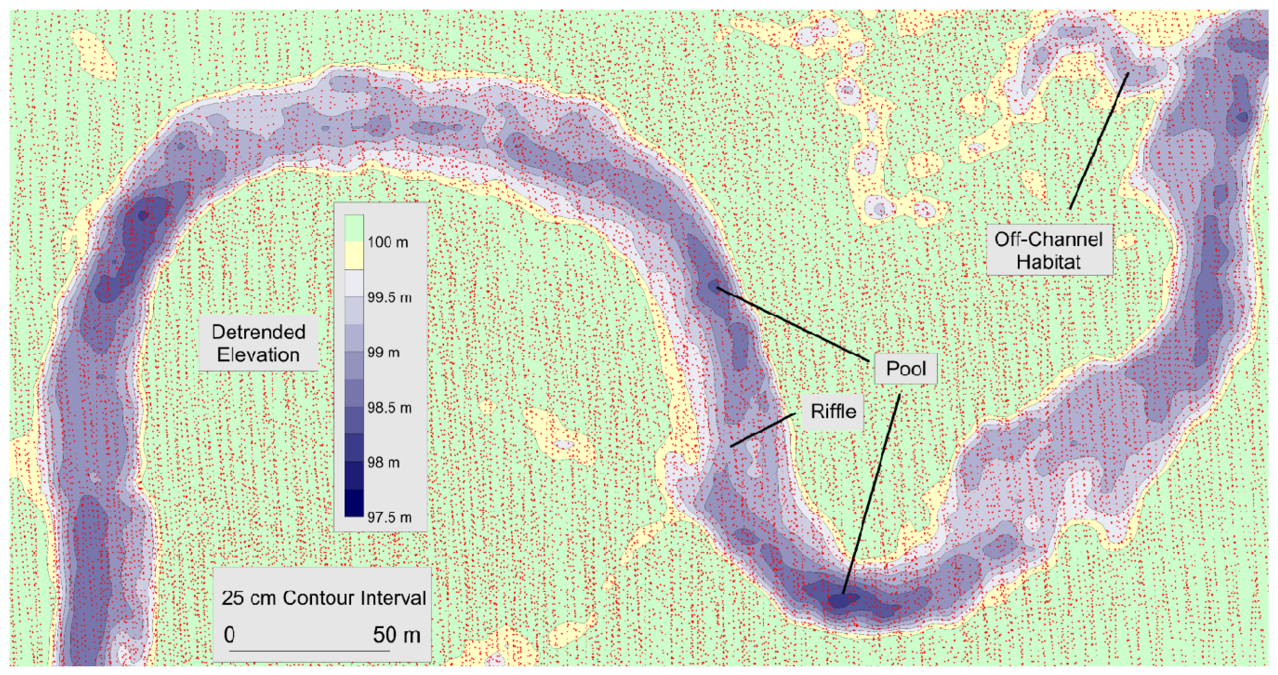
Figure 5 shows a typical contour map constructed from a combination of bathymetric and bare earth data measured by the EAARL over a short reach of a small mountain stream. The down-valley gradient has been removed from these data,
i.e., they have been “detrended” using a procedure discussed later. Most of the contours in the floodplain have also been blanked out except traces of old abandoned channel positions. Examples of major pool and riffle habitat units inside the main channel are indicated as well as the off-channel habitat usable by aquatic organisms only during high flow conditions. With multiple passes over a target area, the sensor delivers data point clouds with sufficient density to construct DEMs with 1–3 m pixel resolution. The data can normally be contoured to a minimum interval of about 20 cm. During a single flight of 4–5 hours duration, nearly continuous data of this quality can be gathered covering 100–200 km of channel length, depending on flying conditions and stream characteristics (primarily water clarity). For comparison, a 2-day ground survey with comparable data density would map only about 200 m of this channel and in many places it would not be feasible to wade the deepest pools.
Figure 5.
Typical bathymetric contours mapped by the EAARL in Bear Valley Creek, ID, USA. Red dots are measurement points made by the EAARL during multiple passes over this reach.
Figure 5.
Typical bathymetric contours mapped by the EAARL in Bear Valley Creek, ID, USA. Red dots are measurement points made by the EAARL during multiple passes over this reach.
By visually comparing contour maps made from the LIDAR bathymetry with basic channel characteristics observed in the field, we have qualitatively investigated the accuracy of EAARL bathymetry in about 40 km of streams and the sensor faithfully maps all major channel bedforms. The largest errors appear at steep or vertical stream banks. The LIDAR is unlikely to reflect from the exact edges of such features and the 20 cm footprint of each reflection is also coarser than an abrupt stream bank edge. Moreover, the geometry of airborne LIDARs means that relatively few measurements are made on the faces or surfaces of steep banks. These effects, in combination with smoothing during data gridding, cause the mapped bank slopes to be too gentle and their edges too rounded in contour maps. Similarly the bottom edges of banks, where they meet the channel bed, are also slightly rounded and occasionally the mapped pools are displaced too far toward the center of a channel. A more quantitative assessment of performance follows.
3.1. Point Elevation Accuracy
The EAARL system has an error budget similar to that of conventional airborne discrete return terrestrial near-infrared LIDARs [
20] with the additional variable of the 1 ns waveform digitizing interval. A bathymetric LIDAR must also account for the 25% decrease in velocity when laser energy moves from air into water. It is difficult to decompose the error budget into its constituents and instead the overall performance of the sensor must be evaluated. The accuracy of EAARL data has been investigated using the standard technique of comparing point elevation measurements by the LIDAR with ground survey points from nearby locations [
6,
9]. In a shallow (generally <1 m deep) smooth sand-bedded river, LIDAR vertical RMS errors relative to a real-time kinematic GPS ground survey averaged 18 cm and 24 cm on exposed and submerged sand, respectively [
9]. A similar comparison in shallow marine and coastal environments found RMS errors of 13.9 cm relative to a boat-based sonar survey in depths less than 2.5 m and 9.9 cm when compared to a wading survey in water less than 1 m deep [
6]. Bare earth RMS elevation errors beneath a variety of coastal vegetation ranged from 16–20 cm [
6].
3.2. Accuracy of Topographic Derivatives
While point elevations are the standard method of accuracy assessment of LIDAR data, for many purposes other topographic characteristics are more important, such as distance, slope, curvature, area or volume of terrain components and spatial arrangement of features. The real power of airborne scanning laser altimetry lies in using the high density of millions of point measurements, made with less accuracy than field measurements but over extensive areas well beyond the scope of field surveying, to describe these higher order topographic features and their spatial arrangement. We have tested the ability of the EAARL system to map several of the common definitions of channel geometry that involve higher order topographic metrics. This work is ongoing and only partial preliminary results are presented.
Data were evaluated at two stream segments, one a simple, straight plane bed reach about 100 m long and the other a 150 m-long meandering reach with more complicated pool-riffle morphology. Both reaches are similar in size, approximately 15 m wide with banks that are about 1 m tall above the mean stream bed elevation. The meandering reach is in an open meadow and the plane bed reach is bounded by a 10 m tall conifer forest with trees at or near the stream banks. They were mapped on the same day by the EAARL and are less than five minutes apart in flight time so data quality is consistent. Intensive field surveys were also made of the test reaches using a total station instrument to map channel bathymetry in internal coordinates. Using survey-grade GPS long-term observations on bench marks, the total station coordinates were converted to the same datum as that of the EAARL instrument. The spacing of the field elevation measurements was about equal to the average LIDAR point spacing and the resulting field-mapped point cloud is the standard against which the LIDAR data were tested. Both the ground survey and LIDAR point clouds were converted to DEMs using an identical isotropic kriging method. The DEM raster cell sizes were 3 m and 2 m respectively, at the meandering and straight reaches.
Data from a series of field measurement points, taken approximately along the centerlines of the channels, were extracted from the original total station point clouds and used to construct reference profiles of channel elevations. Then profiles along the same reference lines were prepared from the separate DEMS constructed using each of the field survey and LIDAR data. The three profiles were qualitatively compared and the reach-average slopes of the beds of the channels were also computed from each profile. The field survey and LIDAR rasters were further evaluated by visually comparing respective contour maps and from a difference image computed by subtracting the LIDAR raster from the control ground-survey raster. The three dimensional surface area of the channel bed and the water volume inside the channel below an arbitrary reference water surface elevation were also calculated from each DEM. Finally, five cross-sections perpendicular to the local trend of the channel were taken from the ground and LIDAR rasters at random locations in each stream reach. The width, maximum depth, ratio of width-to-depth and wetted cross sectional area of each channel cross section were calculated relative to a specified arbitrary water surface elevation.
Figure 6.
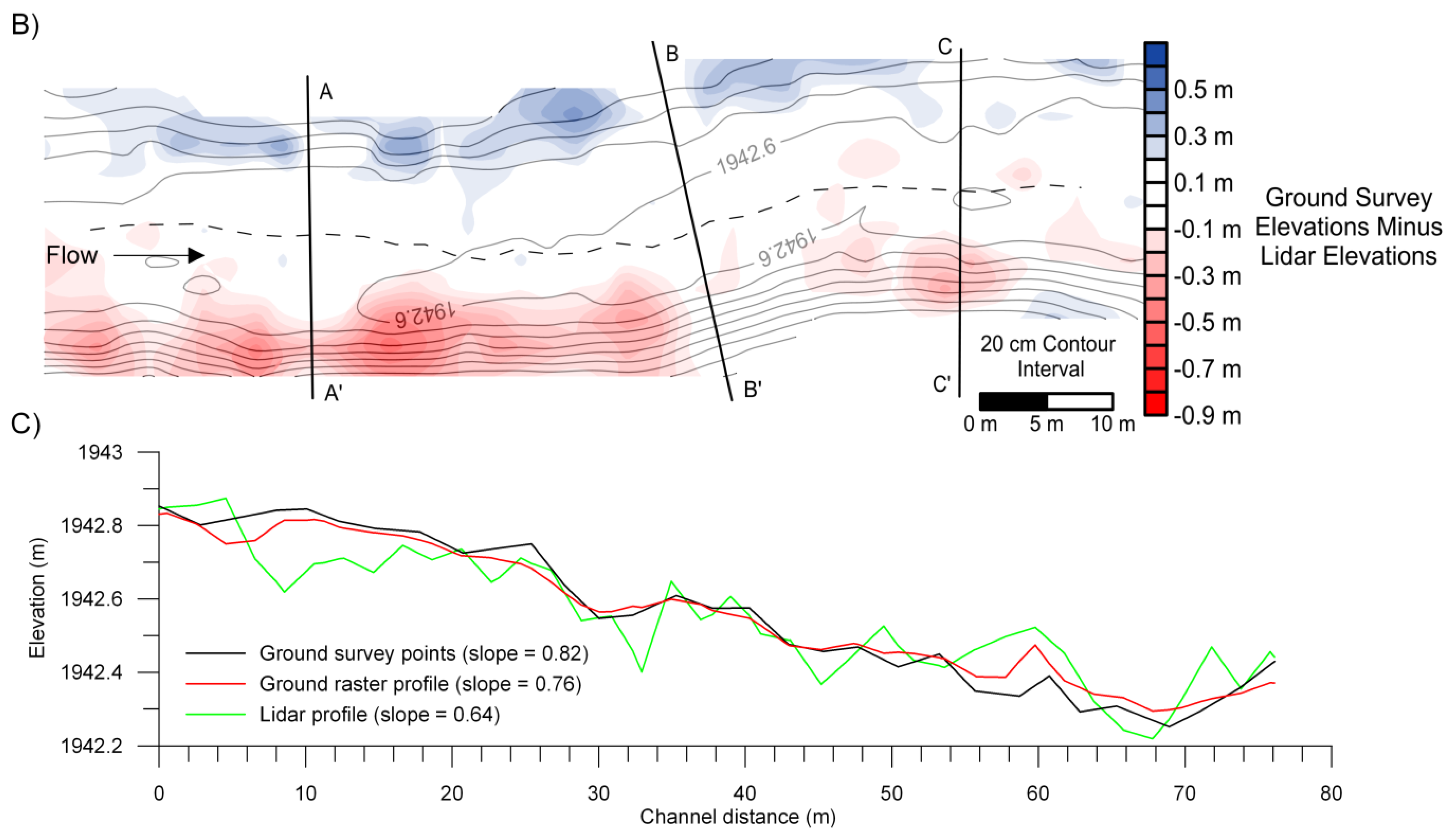
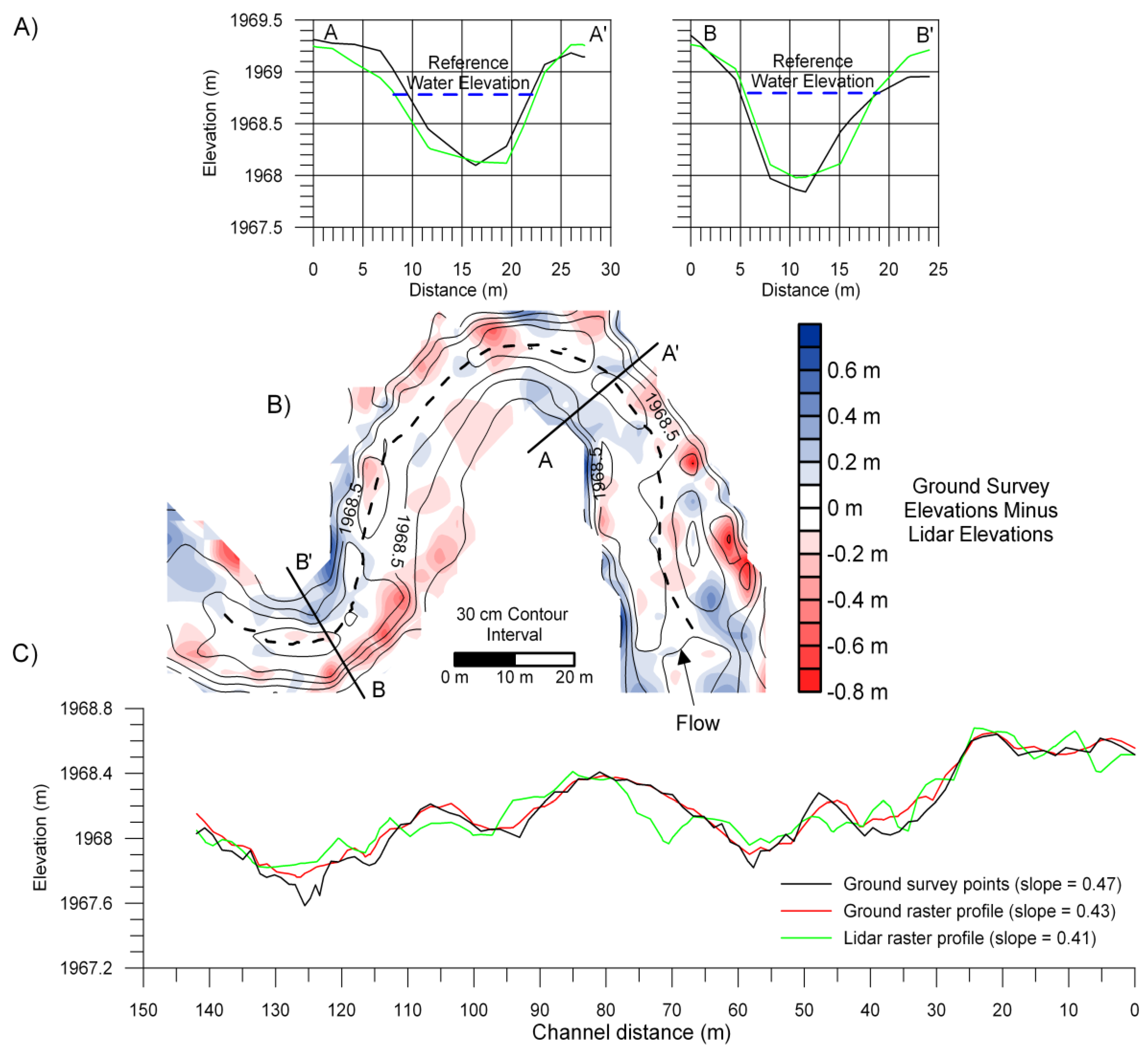
Bathymetric LIDAR and ground survey comparison at a meandering channel reach. (A) Example cross sections at locations shown in map view: black = ground survey, green = LIDAR survey; (B) Map view comparison. The contours are from ground survey data. The colored intervals are elevation differences calculated as ground survey grid node elevation minus LIDAR grid node elevation. These colored intervals are georeferenced to the contour map and show that the largest errors tend to occur along the stream banks. The dashed line is the location of channel elevation profile; (C) Channel elevation profiles: black = ground survey points (most accurate), red = profile through ground survey raster, green = profile through LIDAR raster.
Figure 6.
Bathymetric LIDAR and ground survey comparison at a meandering channel reach. (A) Example cross sections at locations shown in map view: black = ground survey, green = LIDAR survey; (B) Map view comparison. The contours are from ground survey data. The colored intervals are elevation differences calculated as ground survey grid node elevation minus LIDAR grid node elevation. These colored intervals are georeferenced to the contour map and show that the largest errors tend to occur along the stream banks. The dashed line is the location of channel elevation profile; (C) Channel elevation profiles: black = ground survey points (most accurate), red = profile through ground survey raster, green = profile through LIDAR raster.
At the meandering channel reach the LIDAR data appear to map the majority of the channel bed with only small errors (
Figure 6). The largest discrepancies in the map of the channel bed are at a distance of 70 m in the profile plot where the LIDAR has erroneously mapped a 30 cm-deep pool and at distance 125 m where both the LIDAR and ground survey rasters have missed the bottom of a narrow 20 cm-deep pool (
Figure 6C). This small pool is represented in the ground and LIDAR point clouds, but was removed during kriging with a grid cell size of 3 m. Elsewhere on the channel bed the LIDAR bathymetric raster errors are generally in the range of ±10–20 cm. The largest LIDAR errors are along the banks and edges of the channel bed, locations where the topography changes rapidly over short spatial scales. At these sites, the combination of small LIDAR geo-location errors, the 20 cm laser spot measurement diameter and errors introduced during kriging can cause larger elevation mistakes.
Data in
Table 2 compares the basic channel geometry measured by the LIDAR and ground surveys. The reported average channel widths, depths, width/depth and wetted cross sectional areas were calculated using arbitrary reference water elevations as noted in the cross sections shown in
Figure 6A. The LIDAR cross-section widths are slightly larger than those measured in the field and the depths somewhat shallower, resulting in a 9% increase in the width/depth ratio (
Table 2).
Table 2.
Channel geometry comparison by survey methods for a meandering reach with pool-riffle morphology and a straight reach with plane bed morphology. Wetted geometries were calculated below arbitrary water surface elevations.
Table 2.
Channel geometry comparison by survey methods for a meandering reach with pool-riffle morphology and a straight reach with plane bed morphology. Wetted geometries were calculated below arbitrary water surface elevations.
| Channel Attribute | Ground Survey Points | Ground Survey Raster | LIDAR Survey Raster |
|---|
| Meandering Reach | | | |
| Mean X-Section Width (m) | 11.9 | 12.1 |
| Mean X-Section Depth (m) | | 0.7 | 0.7 |
| Mean X-Section Width/Depth | | 16.5 | 18.0 |
| Reach Wetted Area (m2) | | 2,302 | 2,286 |
| Reach Wetted Volume (m3) | | 965 | 1027 |
| Reach Mean Bed Slope | 0.47 | 0.43 | 0.41 |
| Straight Reach | | | |
| Mean X-Section Width (m) | 10.6 | 10.8 |
| Mean X-Section Depth (m) | | 0.4 | 0.4 |
| Mean X-Section Width/Depth | | 32.5 | 31.7 |
| Reach Wetted Area (m2) | | 947 | 976 |
| Reach Wetted Volume (m3) | | 269 | 281 |
| Reach Mean Bed Slope | 0.82 | 0.76 | 0.64 |
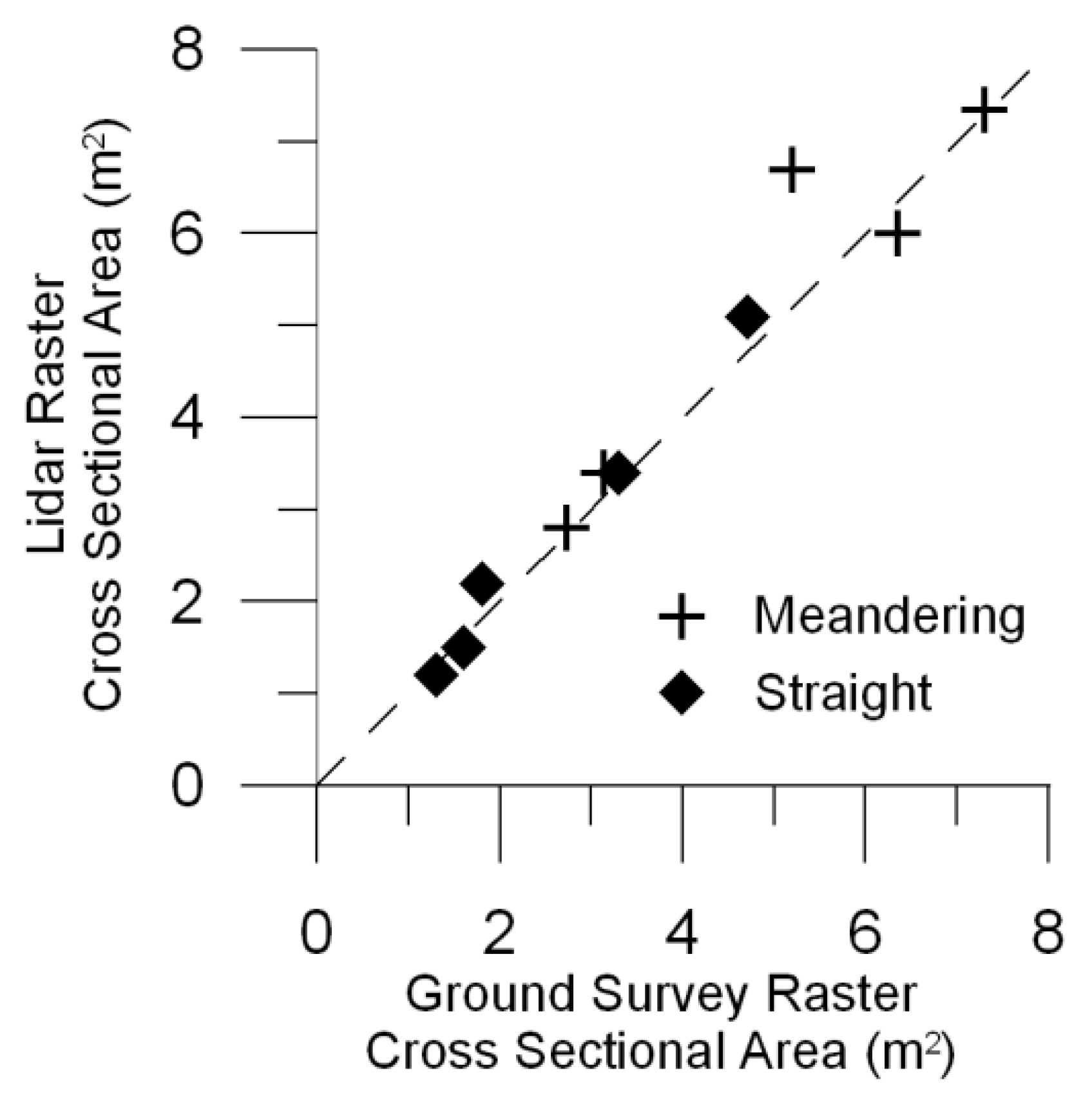
The width and depth errors largely compensate for each other, and the cross section wetted area is close to that defined by the total station survey (
Figure 7). Over the whole reach there is less than 0.7% difference in the three-dimensional wetted areas and less than 6.5% difference in the wetted volumes beneath the reference water surface. Of course these differences in wetted geometry are specific to the arbitrary water surface elevation chosen, but nonetheless are representative of common flow stages between bankfull high flows and very low base flows. The reach-scale average slope of the stream bed is similar in the LIDAR and ground survey raster profiles while the profile of discrete field survey points is a little steeper, because of the previously-mentioned small pool at a profile distance of 125 m, which was not present in the LIDAR- or field-derived rasters.
Figure 7.
Comparison of cross-sectional wet areas below an arbitrary water surface elevation in the meandering and straight channel study reaches, calculated from ground survey and EAARL-derived rasters. Dashed line is a 1:1 correspondence.
Figure 7.
Comparison of cross-sectional wet areas below an arbitrary water surface elevation in the meandering and straight channel study reaches, calculated from ground survey and EAARL-derived rasters. Dashed line is a 1:1 correspondence.
The channel bed in the straight reach has a smooth overall form with no pools, riffles, or other major morphometric units. Again the LIDAR maps the basic channel form well, although more scatter is present in the profile constructed from the LIDAR raster (
Figure 8).
Figure 8.
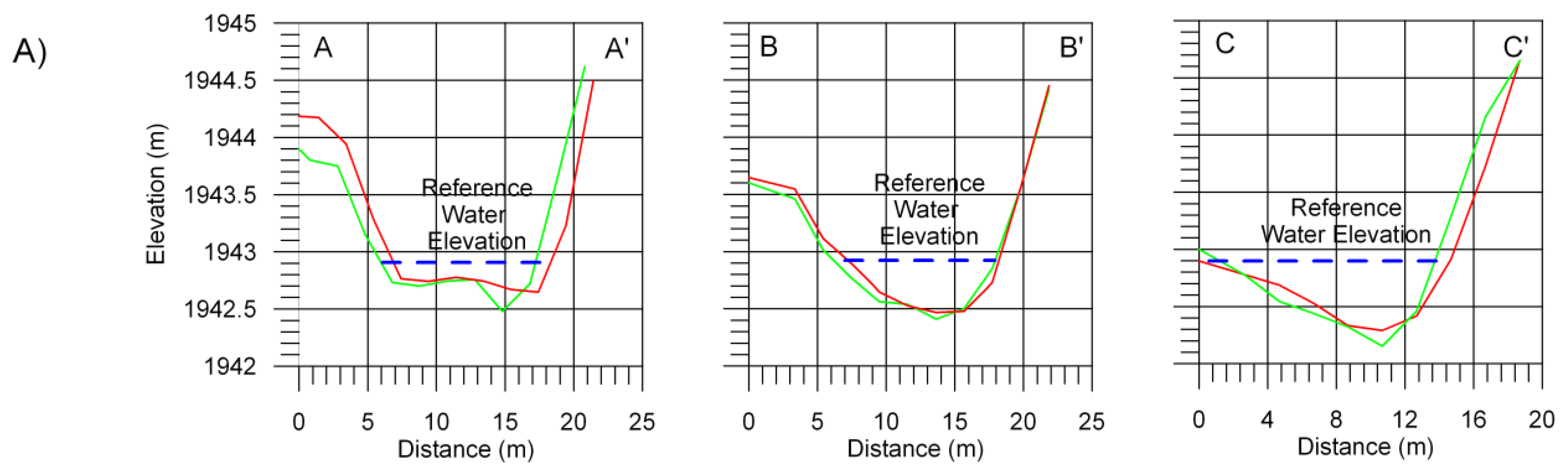
Bathymetric LIDAR and ground survey comparison at a straight channel reach. (A) Example cross sections at locations shown in map view: black = ground survey, green = LIDAR survey; (B) Map view comparison. The contours are from ground survey data. The colored intervals are elevation differences calculated as ground survey grid node elevation minus LIDAR grid node elevation. These colored intervals are georeferenced to the contour map and show that the largest errors tend to occur along the stream banks. The dashed line is the location of channel elevation profile; (C) Channel elevation profiles: black = ground survey points (most accurate), red = profile through ground survey raster, green = profile through LIDAR raster.
Figure 8.
Bathymetric LIDAR and ground survey comparison at a straight channel reach. (A) Example cross sections at locations shown in map view: black = ground survey, green = LIDAR survey; (B) Map view comparison. The contours are from ground survey data. The colored intervals are elevation differences calculated as ground survey grid node elevation minus LIDAR grid node elevation. These colored intervals are georeferenced to the contour map and show that the largest errors tend to occur along the stream banks. The dashed line is the location of channel elevation profile; (C) Channel elevation profiles: black = ground survey points (most accurate), red = profile through ground survey raster, green = profile through LIDAR raster.
The largest error is an approximately 20 cm deep pool mapped by the EAARL but not seen in the ground survey at a channel distance of 6–16 m (
Figure 8C). On average, the other LIDAR elevations on the bed of the channel are correct to within about ±10 cm. There is an approximately 50 cm horizontal offset toward the left bank (looking downstream) in the LIDAR data that produces an underestimate of bank heights on the left bank and a corresponding overestimate on the right bank (see cross sections A and C in
Figure 8A and
Figure 8B). The cause of this translation is unknown and it was not observed at other control survey sites in the field area. This mislocation did not cause large errors in the overall channel bed as it has a planar form, however it may have contributed to some of the errors seen in the LIDAR profile.
The LIDAR measurements of channel width, depth, ratio of width/depth and cross sectional area are all close to those of the field survey (
Table 2 and
Figure 7). In this reach the LIDAR-predicted wetted surface area and volume beneath the reference water surface were within 5% of the values derived from the ground survey. The slope of the bed over the straight reach was slightly less in the LIDAR data due to the previously-mentioned error in mapping the small pool at channel distance 6–16 m.
3.3. Channel Features Mappable with the EAARL
Given the above performance traits, what aspects of channel morphology and physical habitat can be described by this sensor? We have tested the EAARL in recent years by mapping about 300 km of channel in environments ranging from large rivers with steep gradients in deep canyons to small streams in very low gradient unconfined valleys and a river flowing through both urban and agricultural settings. A powerful quality of the EAARL is its ability to resolve small topographic features, down to about 1 square meter in area, while also mapping extensive portions of stream networks, up to several hundred kilometers in length. This ratio of synoptic coverage to resolution gives the instrument a scope of about 10
5–10
6.
Table 3 illustrates the array of characteristics distinguishable by this sensor in many channels. All of these attributes will be automatically retrievable from EAARL-derived DEMs using the GIS-based Bathymetric LIDAR Tool (BLT), which is described in a later section.
Several important physical characteristics are not resolvable in the EAARL terrain data including the topography of undercut channel banks and the location of individual large pieces of woody debris. Piles of logs, or wood jams, with a surface area larger than a few square meters are detectable as well as channel geometry changes caused by woody debris. In fact, wood-forced geometry changes are often of more direct interest than the wood itself. In cases where the wood pieces themselves are important physical habitat, they are normally visible in the CIR and RGB digital imagery.
Table 3.
Channel attributes mappable using the EAARL.
Table 3.
Channel attributes mappable using the EAARL.
| Spatial Scale (m) | Stream Attribute | Comments |
|---|
| 100 | Water depth | |
| 101–102 | Morphologic units (e.g., pools, riffles) | Location, area, volume, curvature |
| | Cross section characteristics | Bankfull elevation, width, depth, area, perimeter, hydraulic radius, asymmetry, thalweg position |
| | Longitudinal profile | Elevation of channel centerline or thalweg, slope (over any distance), changes in other channel characteristics (e.g., width) as a function of distance along channel, frequency domain characteristics |
| | Floodplain and “off-channel” aquatic habitat | Width, perimeter, location, area, volume, slope, stage-dependent connection to mainstem, vegetation characteristics |
| 102–105 | Longitudinal profile | Elevation of channel centerline or thalweg, slope (over any distance), changes in other channel characteristics (e.g., width) as a function of distance along channel, frequency domain characteristics |
| | Planform geometry | Sinuosity, radius of curvature, channel type, etc. |
| | Habitat diversity and complexity | Composition, configuration, complementation, connectivity |
3.4. Effects of LIDAR Errors on Numerical Modeling of Channel Flow and Sediment Transport
One of the more demanding uses of bathymetric data is to define the boundary condition of a channel with sufficient resolution and accuracy to support a computational fluid dynamics (CFD) model. We are testing EAARL data in this capacity using the two-dimensional finite difference fluid dynamics model FaSTMECH, run under the graphical user interface MD-SWMS [
21,
22]. The tests are made on a relative basis by introducing elevation errors in all data in bathymetric point clouds and comparing model performance with and without errors. These investigations are being done in the two previously-discussed stream reaches: one with a simple straight plane bed form and the other a meandering reach with more complicated boundaries and pool-riffle morphology.
The errors are introduced to each EAARL measurement by sampling randomly from a normally distributed error population with a mean of zero and one standard deviation of 10 cm. Experience of one of the authors (Wright) has shown this spatially uncorrelated pattern to be the most likely style and magnitude of error within EAARL data covering a single segment of a stream. The previous results comparing the ground and LIDAR stream profiles (
Figure 6 and
Figure 8) also support this level of introduced error. Next, the original point clouds and point clouds with errors are gridded in exactly the same manner, using kriging, to produce rasters that are then mapped onto the MD-SWMS flow mesh. Using first the original LIDAR topography without errors, predictions are made of the water elevation, flow velocity, and shear stress on the bed of the test channels at three different flow discharges. Other model calibration parameters, such as the fluid flow resistance drag coefficient, are adjusted until model water surface elevations match field observations. Then the modeling is repeated using the LIDAR data with introduced errors and keeping all other model parameters constant. The effects of the elevation errors are evaluated by measuring changes in the three output variables at each node in the flow mesh when the errors are included.
To evaluate the physical significance of changes in the model output variables, we are testing whether the bathymetric errors would lead to a wrong conclusion about a commonly-modeled phenomenon: the shear stress required to mobilize particles on the bed of a channel. This is conventionally considered a stress threshold phenomenon: the local shear stress is either greater or less than a critical value defined by characteristics such as the size and bulk density of sediment grains on the channel bed. In our tests we are searching for sites in the model flow mesh where bathymetric errors would cause the predicted shear stress to switch from above critical to below, or vice-versa.
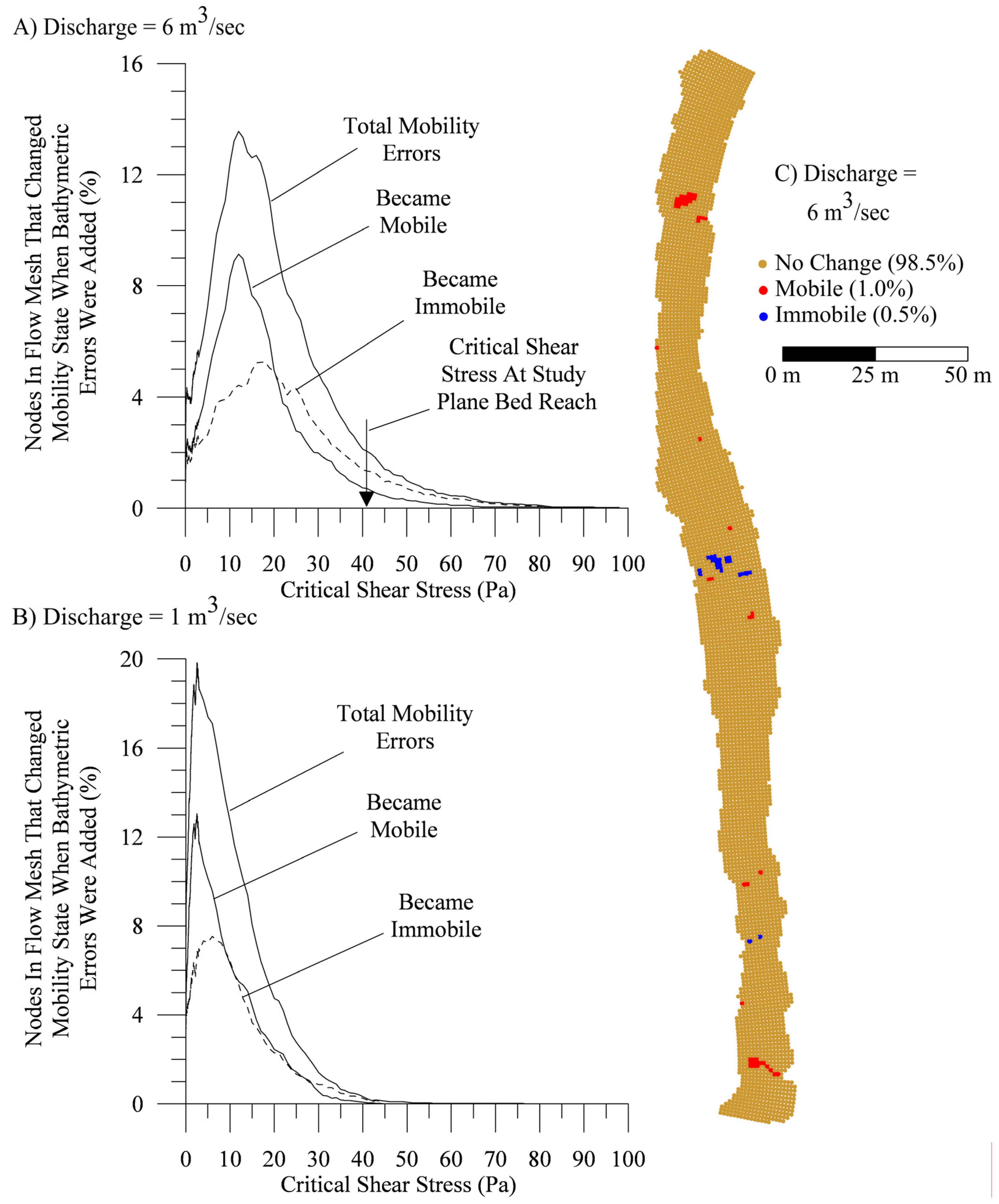
Figure 9 shows a typical result of the bed mobility analysis in the straight plane bed channel reach. Here we have calculated what percent of the flow mesh nodes would switch mobility state with introduced bathymetric errors and repeated the calculation, using the same bathymetric errors, for hypothetical critical shear stress thresholds ranging from 0 to 100 Pascals. Results for high and low flow conditions are shown in
Figure 9A and
Figure 9B, respectively. At both high and low flows the effects of bathymetric errors vary with the hypothetical critical shear stress, but normally cause only a few percent of mesh nodes to switch their mobility condition (
Figure 9A,
Figure 9B). The positions of the peaks in the curves shown in
Figure 9A and
Figure 9B reflect the dominant shear stresses in this reach at high and low flow conditions.
At this stream reach, field sampling demonstrates that the median grain size on the channel bed is gravel particles with a diameter of about 58 mm. A simple bed stability criterion that assumes a single grain size of 58 mm in the channel predicts the threshold of stability to occur at a shear stress of 41 Pa, a typical value for gravel-bed streams. At even the highest flows, the bathymetric errors have little effect at this critical shear stress (
Figure 9A). Assuming a single grain size of 58 mm in the channel, the spatial distribution and sign of the bed mobility errors is shown in
Figure 9C at bankfull flow conditions. Only one percent of the mesh nodes switched from a prediction of immobile-to-mobile and 0.5% switched from mobile-to-immobile as a result of the bathymetric errors. Most of the bed mobility errors occur in areas where the flow was originally quite shallow and consequently the bathymetric errors introduced a relatively large change in the cross sectional area of flow. Simple mass conservation requires that velocity and shear stress vary inversely with changes in the area of flow if discharge remains constant.
Figure 9.
Effects of bathymetric errors on model predictions of bed mobility in a straight, plane bed channel reach. (A) Percent of flow mesh nodes that switched mobility state when flow was the maximum possible inside the channel (6 m3/sec); (B) Percent of flow mesh nodes that switched mobility state at low flow conditions (1 m3/sec); (C) Spatial distribution of changes in mobility state at high flow and using the critical shear stress for bed mobility of 41 Pa that is applicable for this field site. Brown nodes had no change in predicted mobility, red nodes switched from immobile to mobile and blue nodes switched from mobile to immobile.
In summary, our testing to date suggests that EAARL data adequately represent model channel boundary conditions for 1D and 2D fluid dynamics models. In our field areas, the limiting factors in model predictions now appear to be other variables, such as a spatially explicit description of the grain size distribution on a channel bed and the computational efficiency of the models when applied to long stream segments.
4. Derivative EAARL-based Map Products
4.1. Detrended Data
For many purposes, the standard representation of LIDAR-derived DEMs works well, with ground elevations mapped relative to some datum, such as mean sea level. However, a digital representation of a channel normally includes a strong elevation gradient as the channel drops from its source area towards some downstream boundary. While gradient is a very important stream characteristic, it can obscure other significant local topographic features, such as pools and riffles, particularly when mapped stream reaches are several kilometers long. Then it may be advantageous to remove the general channel gradient, or “detrend” the data, for further analyses. Other common stream management applications involve mapping the bankfull elevation, pool depths and volumes, or the extent and depth of floodplain inundation. In a detrended DEM these measures can be directly extracted without the need to generate discrete channel cross sections or run a complex hydraulic flow model. Below, we outline a method for detrending bathymetric LIDAR data, and report our initial validation results.
The most common detrending techniques rely on predetermined functions, such as regression formulas, to identify the data trend. However, in many fluvial settings channel data are nonlinear and nonstationary and detrending processes need to be adaptive to changes in gradient along the data trend. Our method is a variation of the empirical mode decomposition (EMD) procedure [
23] and identifies a trend line between local elevation mean minima and maxima [
24]. Our technique can be optimized for detrending the channel domain only, or for the combined channel and floodplain, if a well-defined floodplain exists. A manuscript is in preparation with a full description of the algorithms.
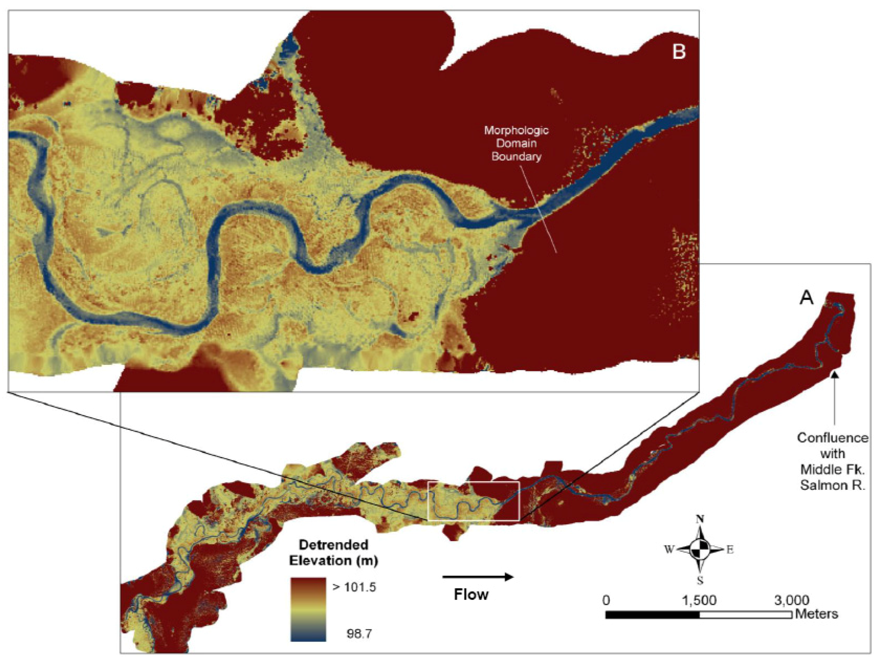
Figure 10 shows a typical result of this detrending method in an EAARL-derived DEM mapping 22 km of channel that begins in an unconfined low-gradient meadow and then flows into a steeper and confined canyon. The transition from the unconfined meadow to confined canyon regime occurs at the Morphologic Domain Boundary. Abandoned and semi-abandoned channel meanders are visible in the meadow north and south of the modern channel. If connected to the main flow during high water stages, these areas are critical off-channel habitat for many species.
Testing of the detrending technique is ongoing but preliminary validation has been completed in a variety of streams by comparing the maximum depths at cross sections in both the undetrended and detrended DEMs. Results to date indicate that for both high and low-gradient streams the average maximum-depth error at a cross section is 2%–3%.
Figure 10.
(A) Detrended DEM of lower Bear Valley Creek, Idaho, USA. The solid field of high elevations in the downstream half of the image is mountains adjacent to the channel which is flowing in a deep canyon through this area; (B) Detailed view of a portion of the detrended DEM. Elevations are relative to an arbitrary datum set during detrending.
4.2. Channel Geometry
Traditionally, hydrologists, geomorphologists and aquatic ecologists have partially relied on a suite of simple geometric measures of channel three-dimensional shape to describe, analyze and manage streams. Example metrics include: (a) the size and shape of the cross sectional area of a channel; (b) the longitudinal slope down the length of a channel; and (c) the planform shape of a stream. These attributes can be easily computed in EAARL-derived DEMs. However, it is difficult to fully exploit the EAARL high resolution digital data by manually making the measurements at scattered locations, because the extensive and continuous LIDAR spatial coverage can easily exceed 100 km of channel length in a single mission. To our knowledge, there is no software that will analyze channel raster data and automatically calculate in-stream morphology and geometry over large channel extents. We are constructing a GIS toolkit that will extract, without manual digitization or measurement, many of the standard hydraulic geometry parameters at user-defined locations in digital data. The Bathymetric LIDAR Toolkit (BLT) is a free extension to the desktop ArcGIS software from ESRI [
25], and will be available on an open website when completed. The tool will operate on any high resolution DEM of a channel, whether made from EAARL data or another source, such as a boat-mounted sonar system or an optical sensor.
Figure 11.
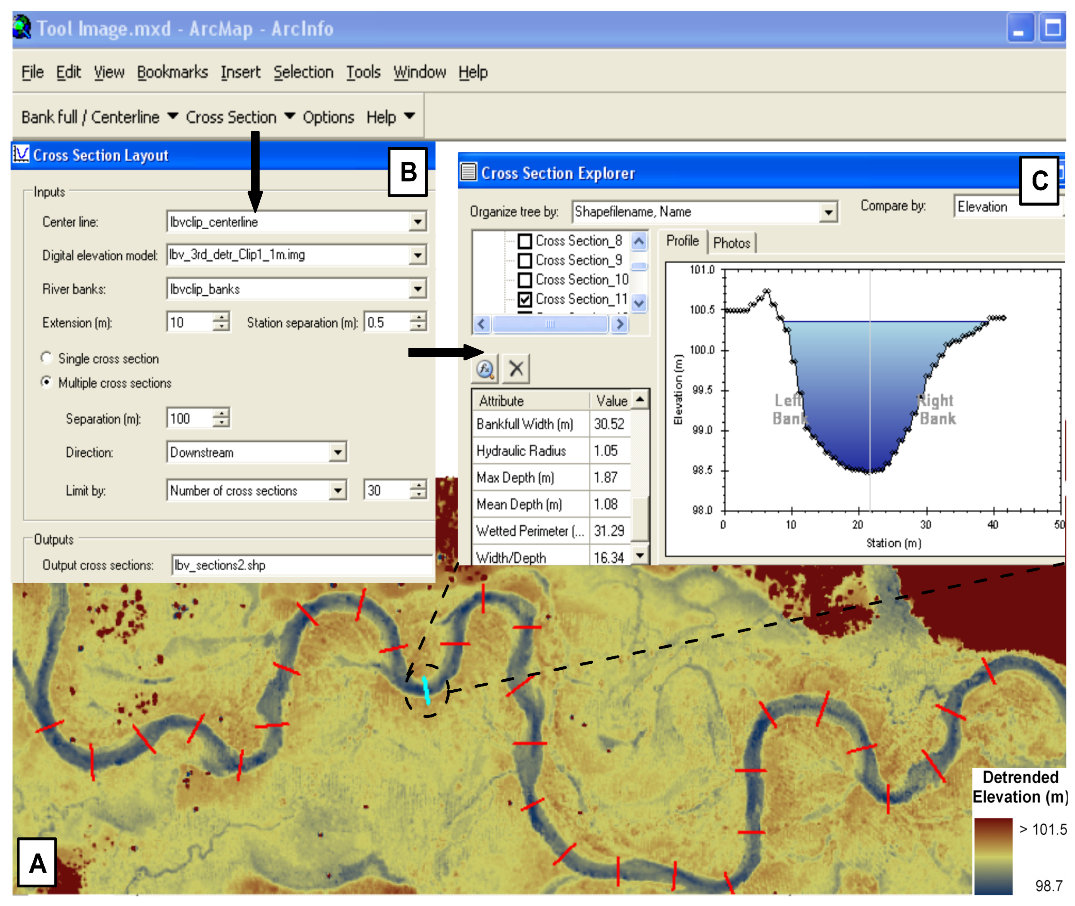
Bathymetric LIDAR Toolkit (BLT) graphical user interface. A) Detrended elevation raster with 1 m grid spacing. Flow is left to right. B) The Cross Section Layout tool provides a variety of methods to define cross section locations. C) The Cross Section Explorer displays the channel hydraulic geometry at single or multiple cross sections.
Figure 11.
Bathymetric LIDAR Toolkit (BLT) graphical user interface. A) Detrended elevation raster with 1 m grid spacing. Flow is left to right. B) The Cross Section Layout tool provides a variety of methods to define cross section locations. C) The Cross Section Explorer displays the channel hydraulic geometry at single or multiple cross sections.
The BLT establishes the channel centerline and then, at user-defined locations, constructs cross sections perpendicular to the centerline. The software next computes a variety of geometric measures at each cross section, including for example the maximum width and depth, the ratio of width/depth, the position of the deepest point in the cross section, the wetted area (A) and perimeter (P) and the hydraulic radius = A/P. In profile down the length of the channel, the slope of the channel bed can be determined and locations of the deepest point in each cross section can be connected to establish a polyline down the path of the deepest flow in the channel, i.e., the thalweg. Changes in other attributes, such as channel width, can also be mapped as a function of distance along a channel profile. In map view, the BLT uses the detrended raster to map off-channel habitat (for example semi-abandoned old channels that are only occasionally flooded at some high flow condition) at any flow stage and define where such habitat reconnects to the main channel. Water levels can be adjusted in the detrended DEM to explore how location, amount and quality of in-channel and off-channel habitat change with the stage of flow.
The BLT graphical user interface is shown in
Figure 11 applied to a small stream mapped by the EAARL in central Idaho, USA. In
Figure 11A the red lines across the channel in the elevation raster are locations of 30 automated cross sections. As defined in the Cross Section Layout menu in
Figure 11B, the cross sections are spaced at 100 m intervals downstream from the initial station which is the left-most section (just above the inset letter A in
Figure 11A). In
Figure 11C the calculated cross section attributes are for a single section (here section 11 shown in blue in the elevation raster). Only a portion of the calculated measures are shown in this example from the user interface. Conventional channel field survey programs normally generate such cross section data from perhaps a few tens of locations. In the BLT it is possible to compile hundreds-to-thousands of digital cross sections in a few minutes.
4.3. Mapping In-Channel and Off-Channel Habitat
In the near future the BLT will be expanded beyond simple measures of topographic geometry and will include procedures to map other in-channel fluvial and aquatic habitat forms and morphometric units, such as the position, area and volume of pools and riffles and the spatial arrangement and connectivity between habitat components.
Figure 12.
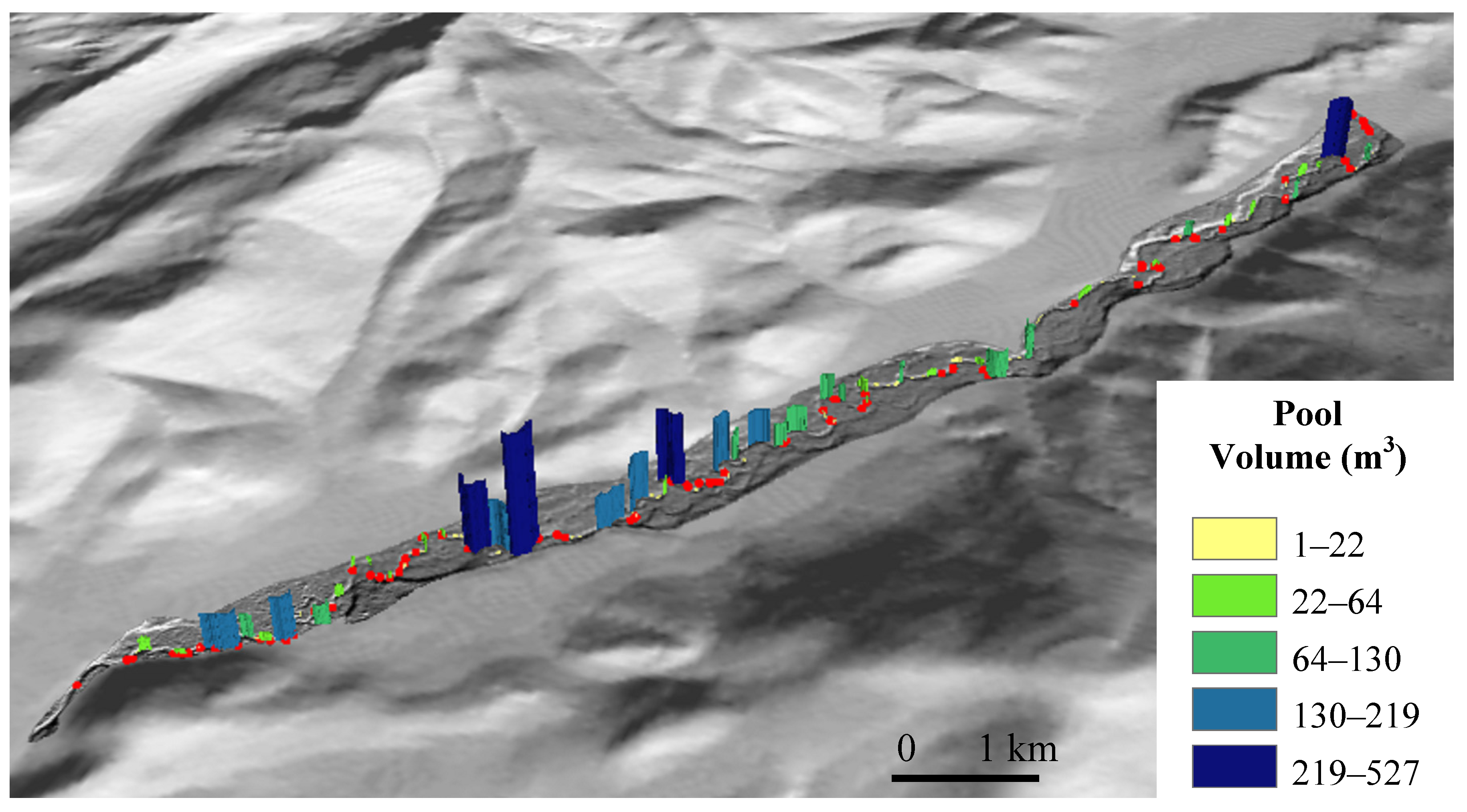
Histogram of pool distribution in upper Bear Valley Creek, Middle Fork Salmon River drainage, ID, USA. The volume of pools was calculated in each consecutive 300 m reach of this 10 km-long stream segment. EAARL data which cover the channel and floodplain are inset in a standard 10 m DEM. Red dots are locations of individual Chinook salmon spawning nests in 2003.
Figure 12.
Histogram of pool distribution in upper Bear Valley Creek, Middle Fork Salmon River drainage, ID, USA. The volume of pools was calculated in each consecutive 300 m reach of this 10 km-long stream segment. EAARL data which cover the channel and floodplain are inset in a standard 10 m DEM. Red dots are locations of individual Chinook salmon spawning nests in 2003.
An example of a possible habitat map is
Figure 12, showing the distribution of pools in a 10 km-reach mapped by the EAARL. The histogram bars display the volume of pools in each 300 m reach of channel. A pool is defined as a concave-upward form in the bed of the channel with a depth greater than 20 cm and surface area greater than 9 m
2, a size definition based on the habitat needs of adult female Chinook salmon who use the pools as resting areas before spawning. The bed concavities were automatically identified in the raster using the Laplacian operator:
Clearly the number and size of pools are not evenly dispersed along the channel with most concentrated in the downstream (left) half of this channel segment. The distribution of spawning sites tracks that of the pools and the salmon spawn in the riffles or crossing between pools. The physical causes of this uneven distribution of habitat are a combination of a glacial legacy and modern channel hydraulics [
10].
In another example, when the EAARL-derived raster is detrended, it is easy to define where and how much off-channel habitat is hydraulically connected to the main channel at any stage of flow by simply raising or lowering a horizontal water surface in the DEM.
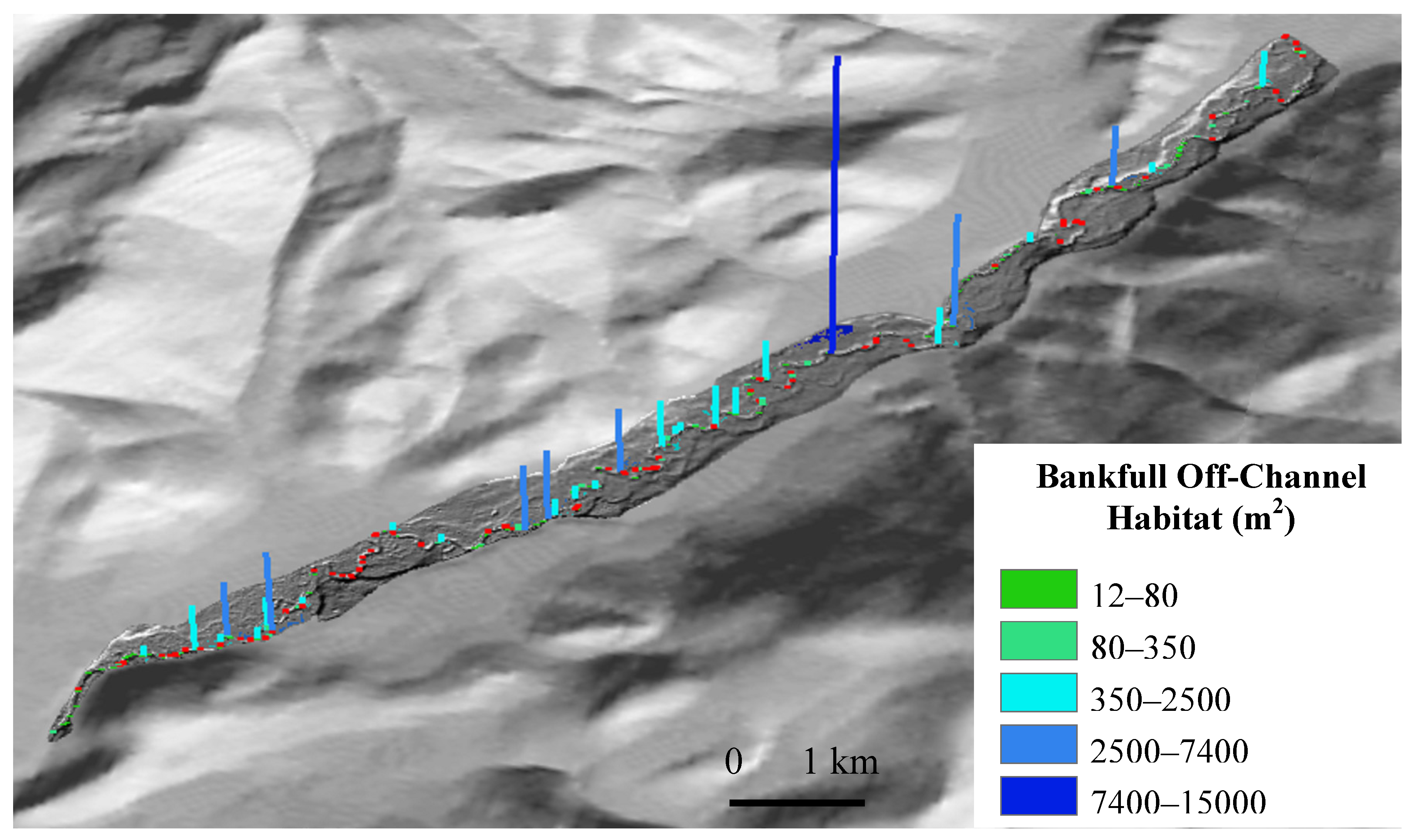
Figure 13 shows the pattern of off-channel habitat in the same 300 m-long reaches of the 10 km channel segment when the flow is at the top of the banks, filling the main channel and off-channel habitat, but not overflowing onto the floodplain. These off-channel areas can be critical habitat. For example, newly-hatched salmon spend much of their first year in the warmer and lower velocity water in these areas. Again this habitat is not evenly distributed, but concentrated in the downstream 60% of the 10 km segment.
Figure 13.
Histogram of distribution of off-channel habitat that is hydraulically connected to the main channel at bankfull flow conditions. Histogram bars show the area of off-channel habitat connected to each 300 m reach of the 10 km stream segment.
Figure 13.
Histogram of distribution of off-channel habitat that is hydraulically connected to the main channel at bankfull flow conditions. Histogram bars show the area of off-channel habitat connected to each 300 m reach of the 10 km stream segment.
4.4. Beyond maps: Frequency Domain Analyses
The continuous spatial coverage of EAARL data over watershed scale stream networks offers the opportunity to examine and describe channels in other ways, including in the frequency domain. There are a variety of frequency analysis techniques such as periodograms, Fourier transforms and wavelet analyses, each with advantages for specific purposes and situations. High resolution channel topography can readily be collapsed to a one-dimensional elevation profile down the length of a stream. These continuous profiles lend themselves well to one-dimensional wavelet analyses to investigate the presence and boundaries of topographic domains that define regimes of physical aquatic habitat.
The wavelet transform is an analytical technique for frequency decomposition of spatial (or time series) data that is particularly useful when the data are nonstationary, as is typical of channel bed topography that often includes many transient signals. Detailed descriptions of the method can be found in several references [
26,
27,
28,
29]. Conceptually a wavelet transform operates by convolving a small reference function, often called the mother wavelet, with the signal of interest. This is a standard convolution in which first the product of the wavelet and a portion of the signal is calculated and that product is then integrated to define a mathematical measure of similarity of that portion of the signal to the reference wavelet. The convolution is repeated as the mother wavelet is both moved along the signal and also dilated or contracted to different spatial scales. Thus the transform is done in space and scale (or frequency) simultaneously. Finally, a measure of spectral power can be computed from the square of the wavelet transform coefficients.
It is a common goal among stream aquatic ecologists and fish biologists to map and monitor the location, size and abundance of spawning habitat for fishes. In the rivers of the northwestern USA, the threatened specie of Chinook salmon (
Oncorhynchus tschawytscha) is a primary management concern. These fish prefer to build their egg nests and spawn on convexities in the channel (riffles) and consequently the form of the vertical profile of a stream bed is an important habitat variable for that life stage [
30,
31]. As an example of the application of this analytical technique, the wavelet transform was used to investigate spawning habitat distribution in EAARL data over the same 22 km-long segment of Bear Valley Creek discussed regarding detrending methods in
Section 4.1. As noted, in this area the stream makes a transition from an unconfined meadow to a narrow canyon (
Figure 10).
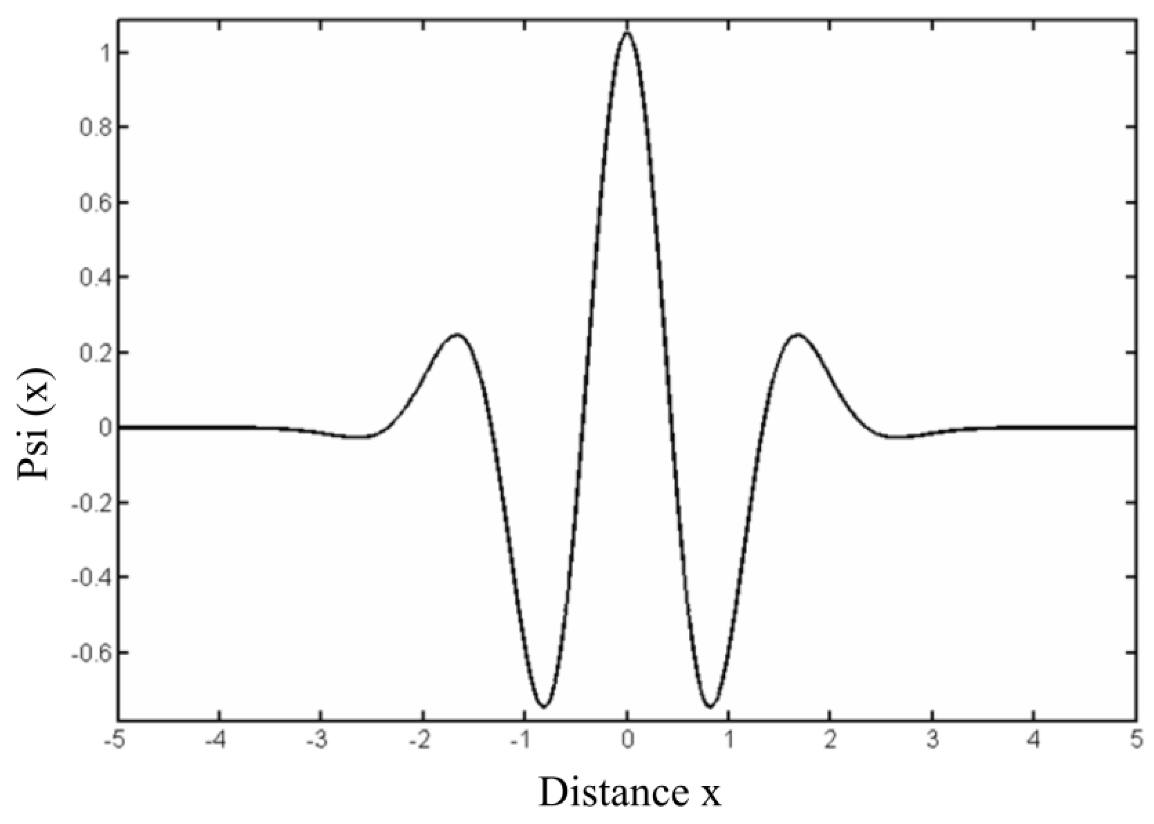
A one-dimensional elevation profile of the channel bed morphology was mapped by hand digitizing the thalweg in the detrended DEM shown in
Figure 10. The transform was done with a 6
th derivative Gaussian wavelet, where the Gaussian is defined as
and the 6
th derivative is shown in
Figure 14. This mother wavelet was chosen because its form resembles a series of pools and riffles as seen in an elevation profile of a stream bed. Similar results are obtained with any mother wavelet that describes smoothly-varying alternate peaks and troughs. When a peak in the mother wavelet is centered on a riffle in the channel profile, the transform coefficients are large positive values and conversely, when a peak in the reference wavelet is on a pool in the profile data, the coefficients become large negative values. In plane bed reaches the transform coefficients tend towards zero.
Figure 14.
Gaussian order 6 wavelet.
Figure 14.
Gaussian order 6 wavelet.
Transform results from the example channel were examined for all spatial scales of the mother wavelet up to 1,500 m long. The selection of a particular scale can be done in a variety of ways, for example by computing the global power spectrum [
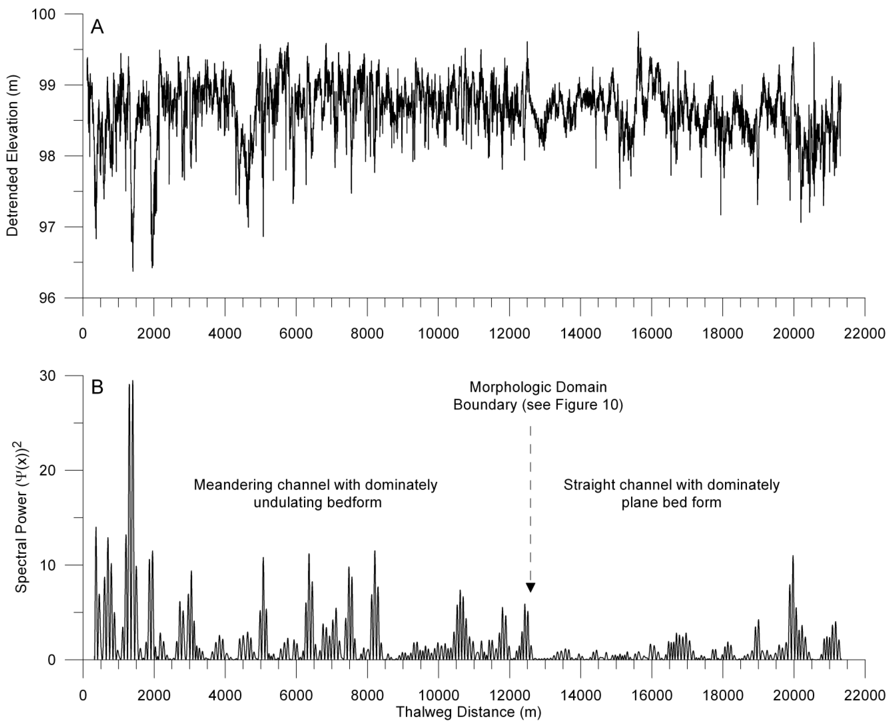
28]. However, the issue at hand is recognition of pool and riffle topography and in a stream this size the typical pool-to-pool spacing is on the order of 100 m. For a Gaussian wavelet with a scale of 100 m, the spectral power distribution over the 22 km-long profile of channel is shown in
Figure 15B. A visual examination suggests the wavelet power defines two domains with a boundary at the vertical dashed arrow. The identified boundary location agrees well with the topography in the detrended DEM (
Figure 10). In the meadow the stream meanders widely and channel hydraulics form a series of pools and riffles, or rhythmic undulations, in the bed, constructing forms suitable for salmon spawning. The magnitude of spectral power varies with the vertical amplitude of the bed forms. To map locations and amplitude of each pool and riffle, the wavelet coefficients could be plotted, rather than spectral power. In the canyon the stream pattern is relatively straight, the bed has few morphologic forms (
i.e., it is a plane bed channel) and the spawning habitat is poorer than in channel segments in the open meadow. The wavelet transform clearly identifies two domains of channel topography and precisely locates the boundary between domains in an objective, quantitative and repeatable manner. While this is a simple example, used for clarity of illustration, in many other cases the wavelet transform identifies spatial patterns that are more difficult to detect using other methods. In particular, this mathematical transform often shows long-wavelength patterns in a channel profile that are not obvious to the human eye.
Table 4 shows descriptive statistics of the thalweg profile wavelet power transform upstream and downstream of the boundary. In the downstream confined canyon the average power drops to only 35% of that in the upstream unconfined meadow. The confined reach of channel also has much more consistent low power levels while in the meandering reach power is quite variable.
Figure 15.
Gaussian (order 6) transform of a channel profile using a wavelet dilation of 100 m. (A) Detrended elevation profile along the channel thalweg; (B) Spatial distribution of spectral power in the thalweg profile. The transition from a meandering pool-riffle channel with undulating bed topography to a straight channel with plane bed topography is noted at the dashed arrow.
Table 4.
Spectral power characteristics of thalweg profile, lower Bear Valley Creek, ID, USA.
Table 4.
Spectral power characteristics of thalweg profile, lower Bear Valley Creek, ID, USA.
| Spectral power | Upstream of boundary | Downstream of boundary |
|---|
| Mean | 1.8 | 0.6 |
| Median | 0.7 | 0.2 |
| 1 std. dev. | 3.1 | 1.1 |
| Minimum | 0 | 0 |
| Maximum | 29.5 | 11.0 |
4.5. Monitoring Change in the Spatial Domain: Some Preliminary Investigations
DEMs derived from airborne LIDAR data generally have poorer horizontal than vertical accuracy, as a result of a combination of: (a) the 20 cm laser reflection spot size: (b) poorer geolocation of each laser point measurement relative to the accuracy of the elevation of the point and (c) spacing of point measurements, which normally is on the order of decimeters to meters and seldom supports DEMs with grid cells smaller than 1 m. Therefore, the horizontal accuracy and coregistration of multitemporal bathymetric LIDAR data may limit how well and what dimensions of channel change can be monitored using this technology. Limited testing has been done of channel monitoring by repeat EAARL surveys with the exception of a project in which changes in the smooth sand-bed Platte River, Nebraska, USA, were successfully mapped over a three-year interval [
32].
Figure 16.
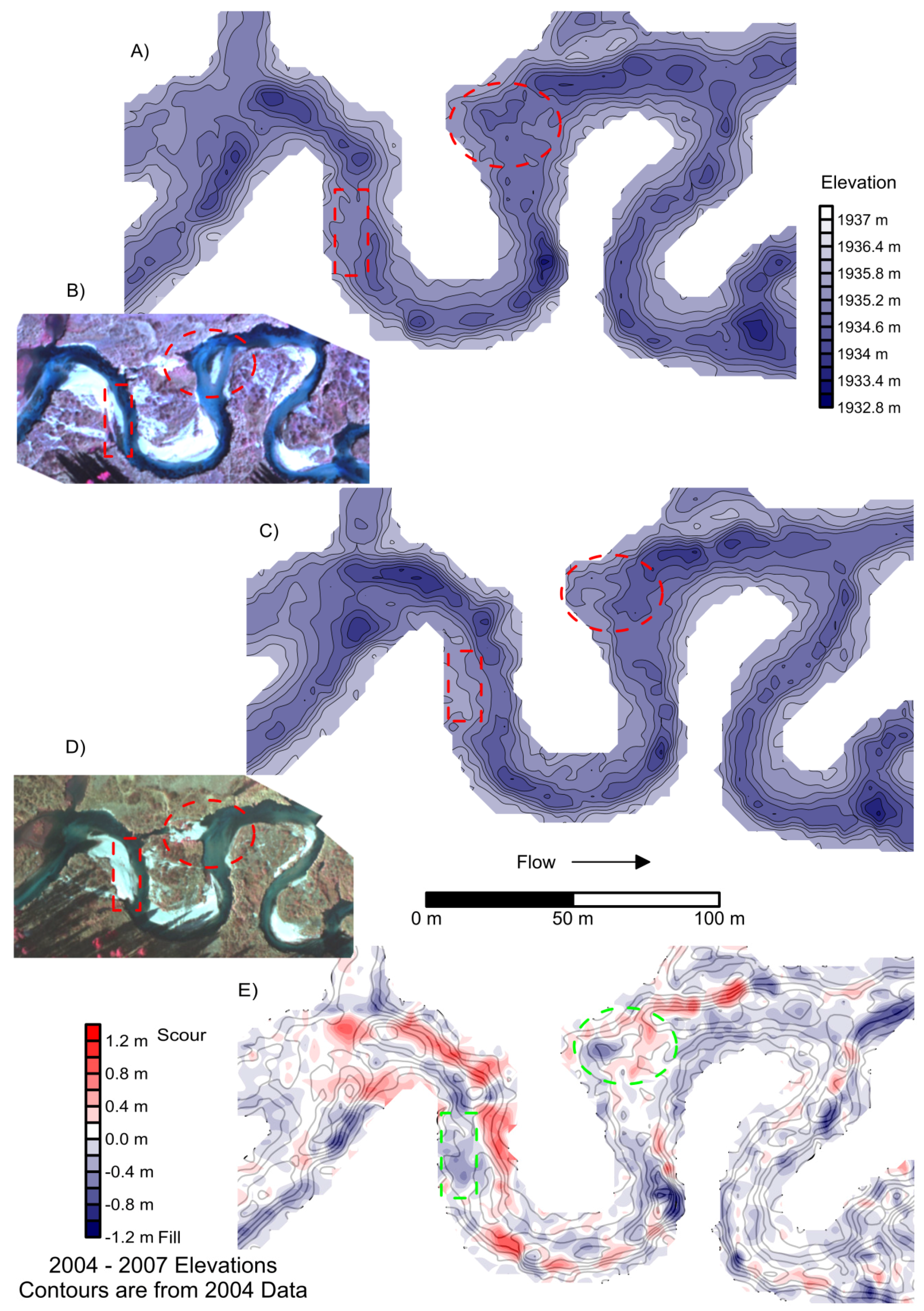
Change in a reach of Elk Creek, tributary to Middle Fork Salmon River, Idaho, between EAARL surveys in 2004 and 2007. Red and green ellipses and rectangles refer to areas discussed in text. (A) Bathymetry in 2004; (B) 2004 CIR photograph; (C) Bathymetry in 2007; (D) 2007 CIR photograph; (E) Colored intervals map the change in channel topography over the three year period, calculated as 2004 minus 2007 grid node elevations. Contours are from the 2004 bathymetric data and are included to give topographic context to the elevation difference values.
Figure 16.
Change in a reach of Elk Creek, tributary to Middle Fork Salmon River, Idaho, between EAARL surveys in 2004 and 2007. Red and green ellipses and rectangles refer to areas discussed in text. (A) Bathymetry in 2004; (B) 2004 CIR photograph; (C) Bathymetry in 2007; (D) 2007 CIR photograph; (E) Colored intervals map the change in channel topography over the three year period, calculated as 2004 minus 2007 grid node elevations. Contours are from the 2004 bathymetric data and are included to give topographic context to the elevation difference values.
In our field area,
Figure 16 is an example of change between 2004 and 2007 in a short reach of a small stream mapped by the EAARL. Each data set was acquired in October of the respective years, during low flow conditions of about 1 m
3/sec, so the water elevation was consistent, within probably a few centimeters, from one data set to the other. While no control field survey data are available, the spatial pattern of erosion is consistent with local hydraulics of such meandering streams with alternating pool-riffle bed morphology. The greatest erosion has been concentrated on the banks along the outside edges of each meander bend. In the area inside the ellipse, the sequential CIR photography shows that a mid-channel bar has been eroded away and a sediment deposit on the left bank (looking downstream) has grown out into the channel during this period (
Figure 16 B, D). The EAARL has correctly identified the sites of both channel bed erosion and deposition, although we are unable to determine the accuracy of the mapped elevation changes without ground survey data (
Figure 16 A, C, E). In the area of the rectangle, a large point bar has extended further out into the main channel and also extended downstream over the 3-year interval (
Figure 16 B, D). Again the LIDAR has correctly identified this area of sediment deposition (
Figure 16 A, C, E). These preliminary results will be extended in the future to include comparison with serial reach-scale ground surveys to better establish the limits and biases of channel monitoring using the EAARL. Again, if most temporal change occurs along the channel banks, rather than in the channel bed, there is greater uncertainty that the EAARL can reliably map and monitor topographic evolution.
5. Discussion
In general, the accuracy of this aquatic-terrestrial LIDAR appears comparable to that of airborne terrestrial near-infrared LIDARs at the scale of point elevation measurements. However, the full power of the EAARL is not developed when mapping point elevations, channel cross sections, or even the topography of short reaches of a stream. Its greatest advantages become apparent when considering longer channel segments and stream networks that are not feasible to map with field surveys. This new capability to map, with relatively high resolution, large portions of channel networks challenges us to think beyond conventional channel cross sections and maps of short reaches of streams, and instead describe and investigate spatial patterns and connectivity of riverine and riparian habitat, aquatic processes and the interactions with channel biota at up to watershed scales.
The airborne EAARL system solves several logistical problems of channel field surveys including ownership restrictions on stream access and mapping in conditions unsuitable for wading due to flow depth and velocity or water temperature. For example, even in the small streams in our primary study area many of the pools are greater than 2 m deep and not accessible by wading with survey equipment.
It is difficult to give general guidance about the costs of EAARL data acquisition and processing. The EAARL is a research instrument and is not used on a high volume of river mapping projects, so an extensive cost history is not available. Furthermore, each project is normally quite unique and costs vary widely depending on factors such as interproject shared mobility costs, flying terrain, dimensions of the survey area, GPS base station availability, channel complexity, vegetation conditions, and density of data required for the purpose of the survey.
Data from the EAARL meet the requirements to map most of the basic physical habitat in channels including the location and size of morphologic units and their spatial distribution and connectivity. The major limitation appears to be an inability to resolve the condition of the banks, for example if a bank is undercut by the stream flow and thus in danger of collapse.
Our investigations suggest that, in many streams, the topographic boundary conditions for 1D and 2D computational fluid dynamics flow and sediment transport modeling can be adequately defined by this bathymetric LIDAR. Model predictions are now limited by other variables such as the “subgrid” scale roughness of the bed or the grain scale roughness, normally estimated by a roughness or friction parameter. However, the EAARL data are not sufficiently accurate for 3D flow models that are much more sensitive to local topography. Currently, this is not a great constraint, as the computational demands of 3D models already restricts their scope to short stream reaches that often could be surveyed by field techniques.
The example 1D wavelet transform gave a clear separation of geomorphic domains, which is an important management and scientific objective. The wavelet analysis could be extended to 2D to explore the full spatial scaling of bedforms defined by the EAARL. There are several other potential applications of wavelet transforms beyond one-time mapping of the scale and frequency of topographic patterns. The method could be used to monitor channel conditions and quantify change over time in channel bed patterns. This is an activity on which land management agencies spend many millions-of-dollars per year using varying styles of field observations and limited channel geometry surveys at local sample sites. In the U.S. alone, additional tens- to hundreds-of-millions of dollars per year are expended restoring river channels to a prescribed geometry. Wavelet transforms could be used to help define the restoration design in the frequency domain and to quantitatively monitor the sustainability of stream restorations.
We have not yet established how well the EAARL will define changes in channel geometry and morphology over time. In common with all airborne LIDARs, the EAARL appears to map changes in elevation better than it does horizontal position of steep surfaces. The result in stream bathymetry is that lateral migrations of channel banks are more poorly defined than are changes in channel bed elevations. Thus, an example of an optimal application of monitoring using the LIDAR would be to observe evolution of the channel bed after a significant change in sediment supply to a stream. If the sediment supply increased, this might result in general bed aggradation, or could affect only some morphologic units; the pools could begin to fill with trapped sediment, even though the riffles between pools remained unchanged. The question remains of what is the threshold of bed elevation change that can be reliably detected and mapped. At the channel margins, our experience is that a vertical bank would have to move laterally on the order of 50 cm before the current EAARL sensor could reliably detect that migration in the digital terrain data. It is probably preferable to monitor lateral shifts in channel position and bank migration using the high-resolution CIR camera data by coregistering multitemporal imagery. The approximately 15 cm-pixels in the imagery have about an order of magnitude better horizontal resolution than do the cells in a typical DEM constructed from the LIDAR data.
While the EAARL seems a major advancement in shallow bathymetry of streams, several impediments remain to routine channel mapping with this sensor. When the water is too shallow (less than about 20 cm deep), a reflection off the air-water interface will often be convolved with a bed reflection in the same waveform, as the two occur too close in time. A combination of hardware and software modifications may be required to resolve this issue.
In the current data handling scheme, all data are first processed in a subaerial bare earth mode and then again all in bathymetric mode, as if the whole landscape was underwater. Next a polygon is established that separates the surface water domain from the subaerial portion of the landscape, using a trial elevation raster and other information, such as the mission imagery, to guide the stratification. Finally the bathymetric data from inside the polygon are combined with the subaerial bare earth data from outside the polygon to form a combined subaqueous-subaerial bare earth point cloud. This process is tedious in data that covers tens- to hundreds-of-kilometers and especially so with a meandering channel and isolated water bodies in the floodplain. It may be possible to integrate the CIR imagery into this work flow and classify the surface water bodies in the CIR data, thus automating the separation of bathymetric and subaerial domains in the LIDAR data.
Accurate definition of the stream banks is also complicated by the presence of vegetation at the edge of a channel. Most filters used to separate vegetation reflections from bare earth returns in airborne LIDAR data do so by searching for unusual departures from local elevation trends, for example a reflection from the top of a bush that stands 1 m above the surrounding ground. However, when these schemes are applied to bathymetric data, the filters often misidentify as vegetation the abrupt rise in elevation from a channel bed to the top of a steep stream bank. Consequently, manual editing is commonly used to remove vegetation returns from bare earth reflections along the edges of channels. Better automated and more efficient procedures are needed to replace manual editing.
The majority of our projects with the EAARL have been in channels with relatively clear water. But suspended sediment and entrained air bubbles in the water column are both point reflectors that prevent a portion of the transmitted laser energy from reaching the channel bed. Some dissolved organic molecules also appear to absorb the green laser energy. More work is needed to investigate the limits of water quality, beyond which stream bathymetry is not possible with this sensor. To our knowledge, the only preliminary data pertinent to this question are from an EAARL survey of the lower Boise River, Idaho, in 2007. Here water quality was measured during the LIDAR mission and initial assessments of the data indicate that water penetration by the laser energy was incomplete when turbidity reached somewhere between 4.5 and 12 Nephelometric Turbidity Units (NTUs), which is a standard measure of water quality [
33].
The full-waveform EAARL data also have great application to the investigation of the three-dimensional structure of vegetation. This subject is beyond the scope of the current manuscript but further information about the investigation of vegetative structure using full-waveform, narrow-beam terrestrial-aquatic and terrestrial airborne LIDARs can be found in sources such as [
15,
34,
35].
6. Future System Development
The EAARL system is currently being upgraded to improve measurement of bathymetry in shallow streams. Enhancements include a more powerful laser with a greater pulse frequency and shorter pulse width, an integrated GPS-INS receiver and a high-speed multichannel waveform digitizer. These components should produce about six times greater data density, better water penetration, improved ability to discriminate water surface reflections from bed reflections, better overall accuracy and better spatial resolution of small topographic features.
7. Conclusions
It is now possible in single integrated airborne missions to acquire relatively high-resolution cross-environment data describing stream bathymetry, floodplain bare earth topography and vegetation three-dimensional structure. The EAARL also allows us to investigate this integrated environment of channels and floodplains and the interactions across physical and biological domains over a greatly expanded range of spatial scales; from aquatic microhabitats covering a few square meters of a stream bed to major portions of channel networks in whole watersheds.
This potentially powerful combination of high-resolution, expansive, aquatic-terrestrial information challenges us to develop new analytical techniques that will fully exploit these unusual data. Are there new insights and understanding of processes and system response to external perturbations or internal instabilities that will be revealed if we move beyond considering channels at the scale of multiple individual points, cross-sections, or short reaches? For example, will better knowledge of habitat distribution and connectivity at scales greater than a kilometer-long channel segment significantly improve our understanding and management of streams and floodplains?

