1. Introduction
The snow cover in high latitudes exerts a strong forcing on the exchange of energy and gases between the surface and the atmosphere. Snow cover modifies the albedo, thus strongly affecting the absorption of short wave radiation. It also thermally insulates the soil surface from the atmosphere, thus modifying the temperatures at the soil surface. Snow cover also affects the gas exchange, as during the winter gases emitted from the soil (e.g., carbon dioxide and methane) have to diffuse not only through the soil, but also through the snow-pack.
In high latitudes, the springtime evolution of biological activity is often closely linked to the increase in temperature. As the vegetation phenology and the timing of the disappearance of the snow cover both depend on the temperature conditions, their interannual variations are likely to be correlated. Aurela
et al., [
1] and Grøndahl
et al., [
2] have even observed that the annual carbon balances of northern ecosystems are correlated well with the disappearance of the snow cover. Thus the timing of snow melt is a parameter that could be used in carbon exchange models.
As the surface observation network in high latitudes tends to be sparse, methods for remote observation of the timing of snow melt would be beneficial. Remotely-sensed snow cover maps could be one useful tool for this. Remote snow cover mapping can be conducted using e.g., the normalized difference snow index (NDSI) based on the visible and middle infrared channels [
3,
4]. Recently, weekly surface albedo data (SAL) from the Satellite Application Facilities within EUMETSAT have become available [
5]. Since there is a close connection between the surface albedo and snow cover [
6], we can assume that the previous parameter can be used to monitor changes in the latter.
The aim of this paper is to present a simple method for determination of the timing of the spring-time disappearance of the snow cover using remotely-sensed weekly surface albedo. To validate the method, we also compare its results to the timing determined using snow depth measurements.
2. Materials and Methods
Weekly mean values of surface albedo based on NOAA/AVHRR [
5] were acquired from the website of the of the Climate-SAF project (
www.cmsaf.eu). The weekly mean value of each pixel is the average of all available instantaneous cloudfree albedo values normalized to correspond to a sun zenith angle of 60 degrees. The sun zenith angle was required to be smaller than 70 degrees and the satellite view angle smaller than 60 degrees. Thus the number of independent albedo values included in the weekly mean depends on the cloudiness and the latitude. Data from the years 2005 and 2006 were used. The area used in the study is bounded by latitudes 55° and 75°N and longitudes 0° and 45°E, thus covering the area of Northern Europe.
Use was made of data from snow depth measurements carried out routinely by Finnish Meteorological Institute at 379 weather stations all over Finland in the same years. These weather stations lie between latitudes 59°46’N and 69°46’N and longitudes 19°52’E and 31°04’E. Albedo data measured locally at two sites, SMEAR II [
7] and Siikaneva [
8], both in Southern Finland, were also used. At the stations the snow is measured at one fixed point. The snow observation value is given as zero, when there is no snow at the measuring stick, but still some snow in the near surroundings. When the snow has completely melted the value is given as −1.
The temporal resolution of the remotely-sensed and locally-measured data is quite different. The remotely-sensed albedo product has a weekly resolution, whereas the local surface observations are made daily (snow depth) or hourly (albedo). In addition, the local surface albedo and snow depth refers to a small area on the scale of a meter, whereas the remotely-sensed albedo is derived for an area of 15 km × 15 km.
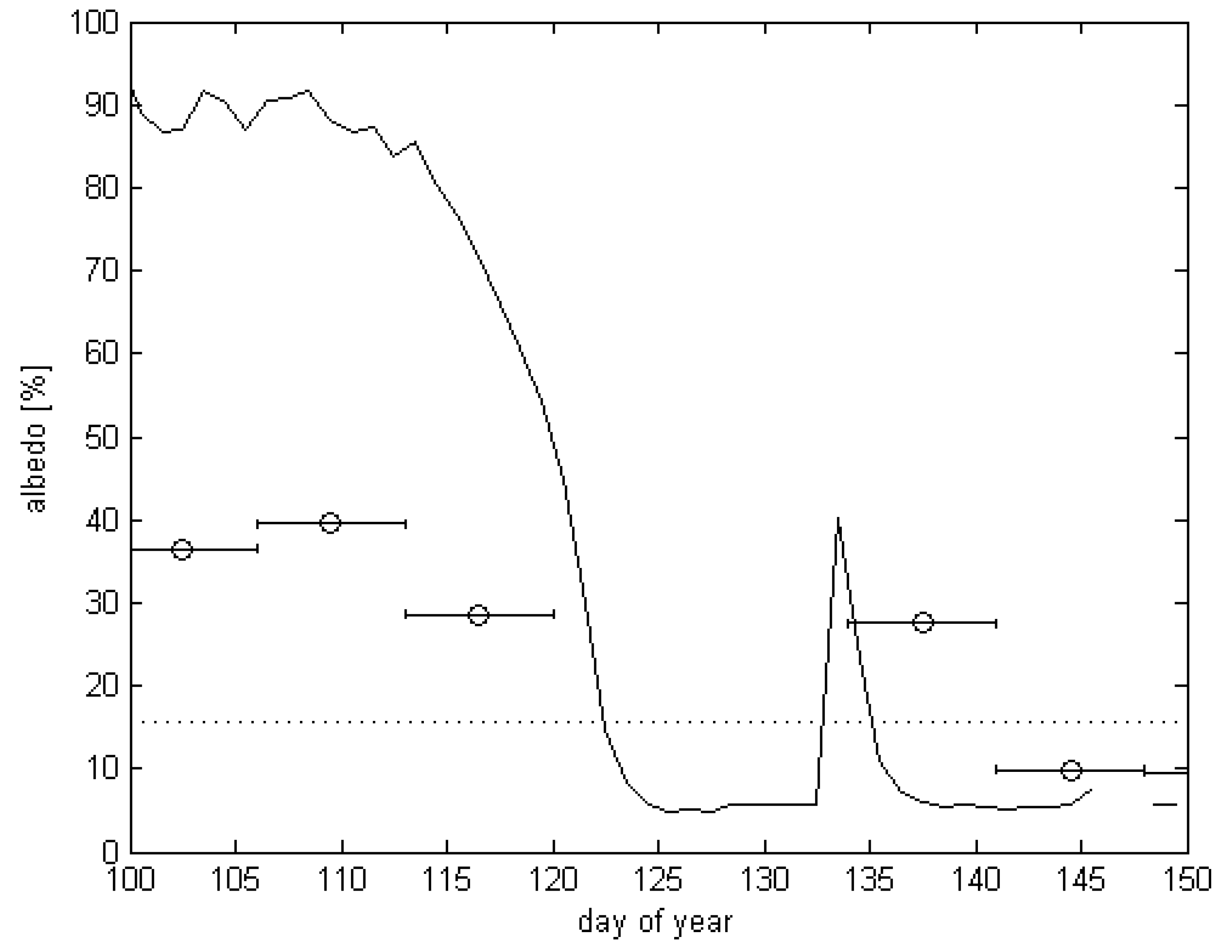
The surface albedo has a large spatial variability, due to differences in land cover within each 15 × 15 km grid box, as can be seen in
Figure 1. The albedo measurements at the Scots pine forest site (Hyytiälä), presented in this figure, were conducted at the SMEAR II research station [
7] 70 meters above the surface. The measurements at the Siikaneva site [
8] were conducted above an open fen ecosystem 1 meter above the surface. Especially during the period of snow cover the albedo differences between the coniferous forests and open areas, such as wetlands and agricultural areas, are pronounced. The summertime differences are also significant. However, at most places the local temporal summertime variation is much smaller than the spatial variability.
Figure 1.
Time series of albedo values in Southern Finland in 2006. The coordinates of the selected SAL grid square are 61°48’N, 24°11’E. Siikaneva (61°50’N, 24°12’E) and Hyytiälä (61°51’N, 24°17’E) are surface observation sites within the selected SAL grid square that are located in an open wetland and a Scots pine forest, respectively.
Even though the absolute albedo values, measured over different ecosystems or from a satellite, differ significantly, a sharp drop in the values is observed in connection with the disappearance of the snow cover (
Figure 1). Thus the timing of this drop in remotely-sensed albedo can be used to determine the disappearance of the snow cover. Below we present a method for determining the timing of the disappearance of the snow cover, or snow melt day (SMD), from the local change in remotely-sensed albedo. The SMD is determined as the first day on which the albedo in the specific grid cell falls below its specific threshold value. As the temporal resolution of the SAL data is one week, we linearly interpolated the SAL data to yield data with an apparent resolution of one day, and used these to determine the SMD.
As there is some temporal variation in the summertime albedo due to, e.g., changes in vegetation cover and leaf status, the threshold which the albedo had to pass,
At was set to:
where
As is the average albedo over July and August and
σAs the standard deviation of this value. By calculating the threshold values and determining the snow melt days separately for each pixel the difficulties arising from the spatial variability in surface characteristics can be bypassed. The method described above was applied separately to all pixels in the data covering Northern Europe for the two years (2005 and 2006) for which we had SAL data available.
In order to validate the method based on remote sensing, the timing of the snow melt was also determined using snow depth data from the synoptic weather observation network in Finland. Here the SMD was determined as the day when the snow depth was 0 cm for the first time in spring. Thus both methods ignore snowfalls later in the spring, which can accumulate some snow for a short period of time.
The method described above can only be used to obtain the timing of snow disappearance a few months after the event, as it requires information on the summertime albedo. Hence it is best suited for research rather than for operational use. However, we studied the possibility of estimating the time of snow melt using the summer-time albedo values from the previous year. In this modification we determined the average summertime albedo value for every SAL pixel using 2005 data. The timing of snow disappearance in the subsequent spring, 2006, was then determined as the time when the albedo value had fallen below the threshold determined from the previous year’s data.
3. Results and Discussion
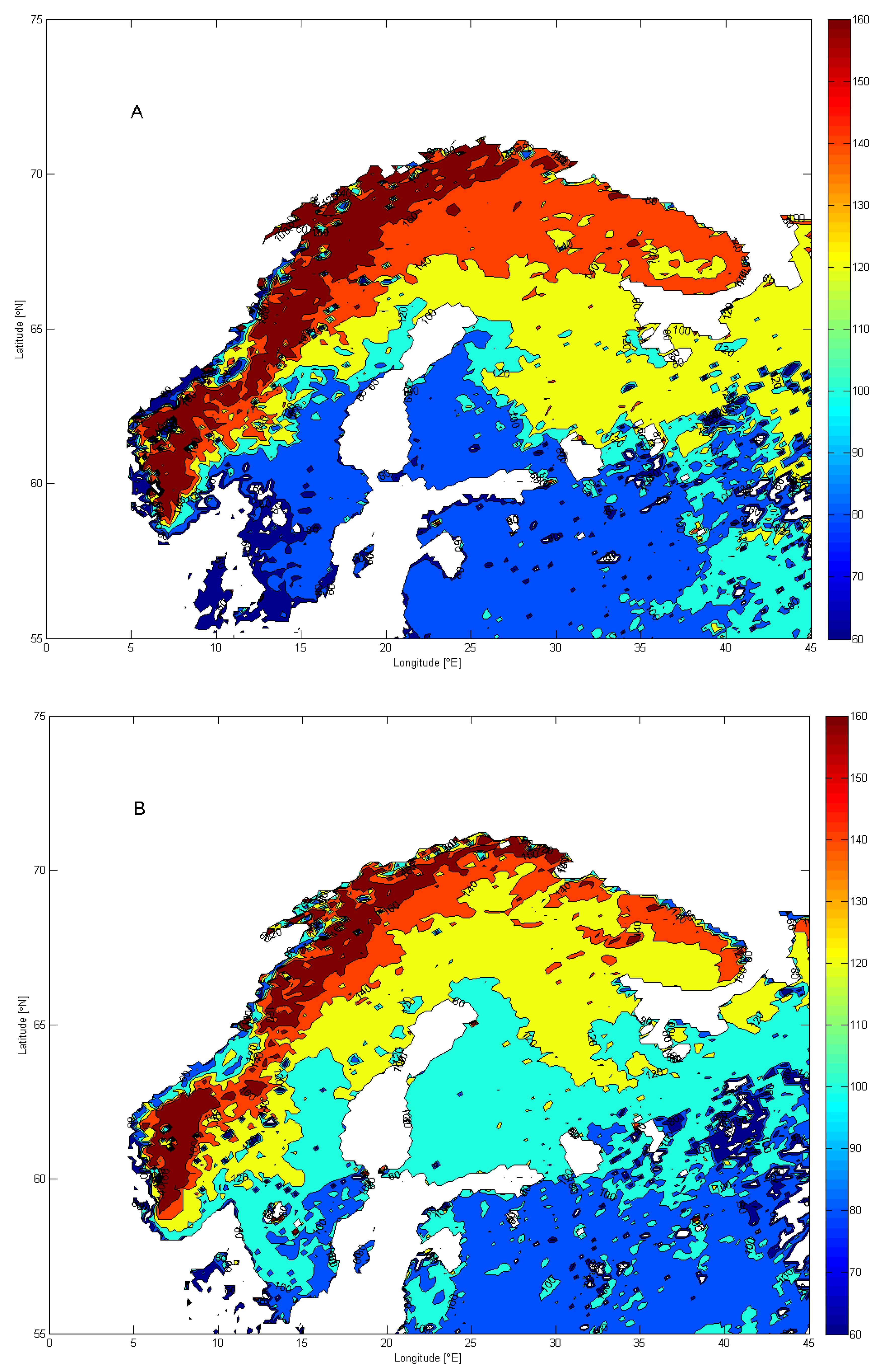
The spatial distribution of the timing of the snow melt (
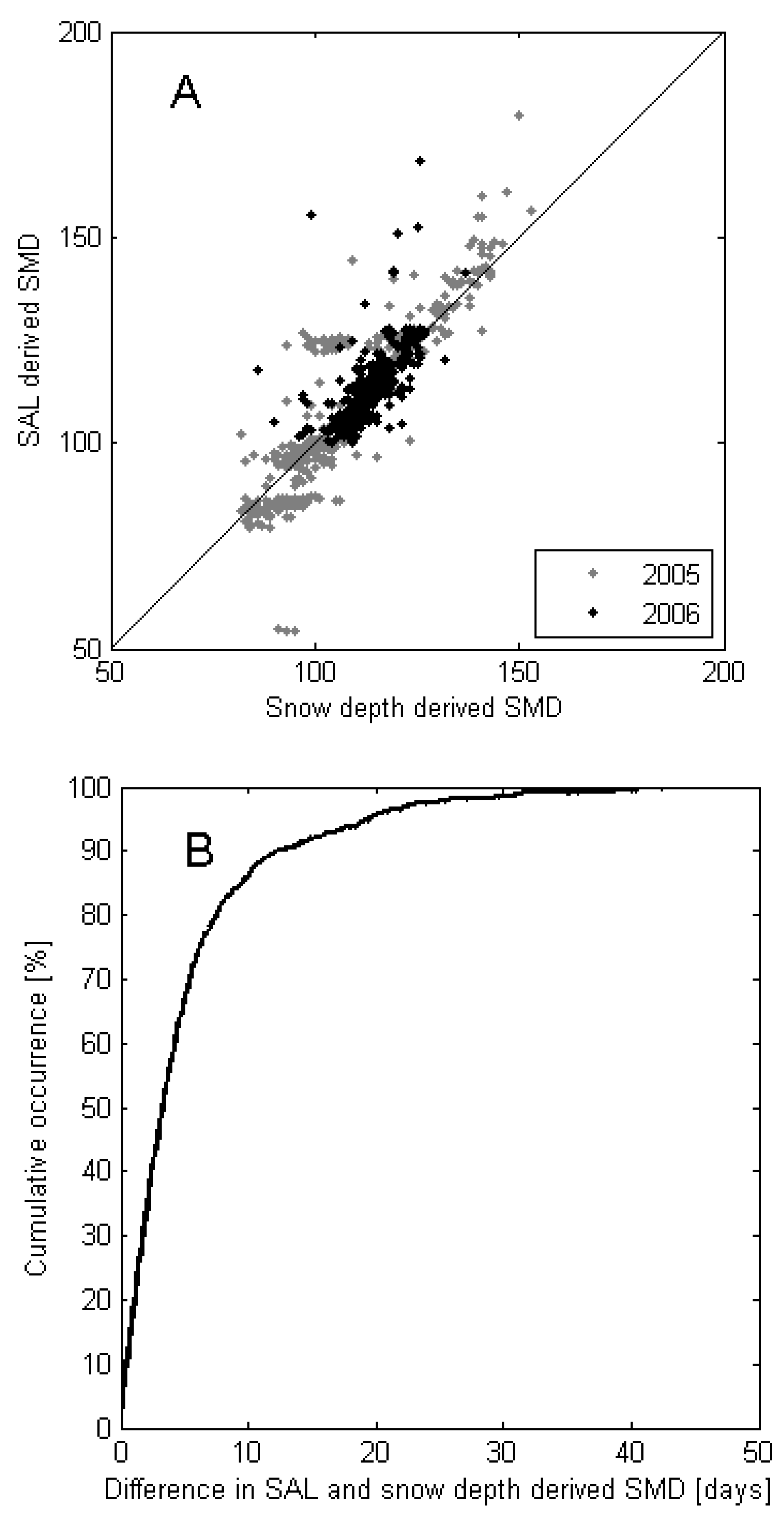
Figure 2) shows a reasonable pattern with early snow melt in the south and low-lying areas, and late snow melt in the north and high mountains. Also the differences in timing between the two years are remarkable. The correlation between the snow melt dates based on the remotely-sensed albedo and on local snow depth measurements is reasonably good (r = 0.87;
Figure 3A), and the slope showing nearly one-to-one relationship (1.05). The average difference between the SMD derived using the SAL product and that from the snow depth observations was less than half a day, indicating the minimal bias of the method. The mean absolute difference between the remote sensing and local snow depth measurement SMD values was 5.4 days. By calculating the cumulative error distribution (
Figure 3B), we can see that in half of the cases the difference was 3.4 days or less. Since the weekly mean albedo value, based on remote sensing, may be dominated randomly by any day during the week because of cloud cover variation, it is not reasonable to expect a much higher temporal accuracy for the remotely-sensed SMD estimate.
Figure 2.
Snow melt day in Northern Europe as derived using the SAF surface albedo product in 2005 (Panel A) and 2006 (Panel B).
Figure 2.
Snow melt day in Northern Europe as derived using the SAF surface albedo product in 2005 (Panel A) and 2006 (Panel B).
Figure 3.
(A) Snow melt day (SMD) as derived using the SAL surface albedo product plotted against that derived from surface snow depth measurements. The grey dots are observations from the year 2005 and the black ones from the year 2006. The solid line indicates the 1:1 relation; (B) Cumulative distribution of the absolute differences between SAL and snow-depth-derived SMD.
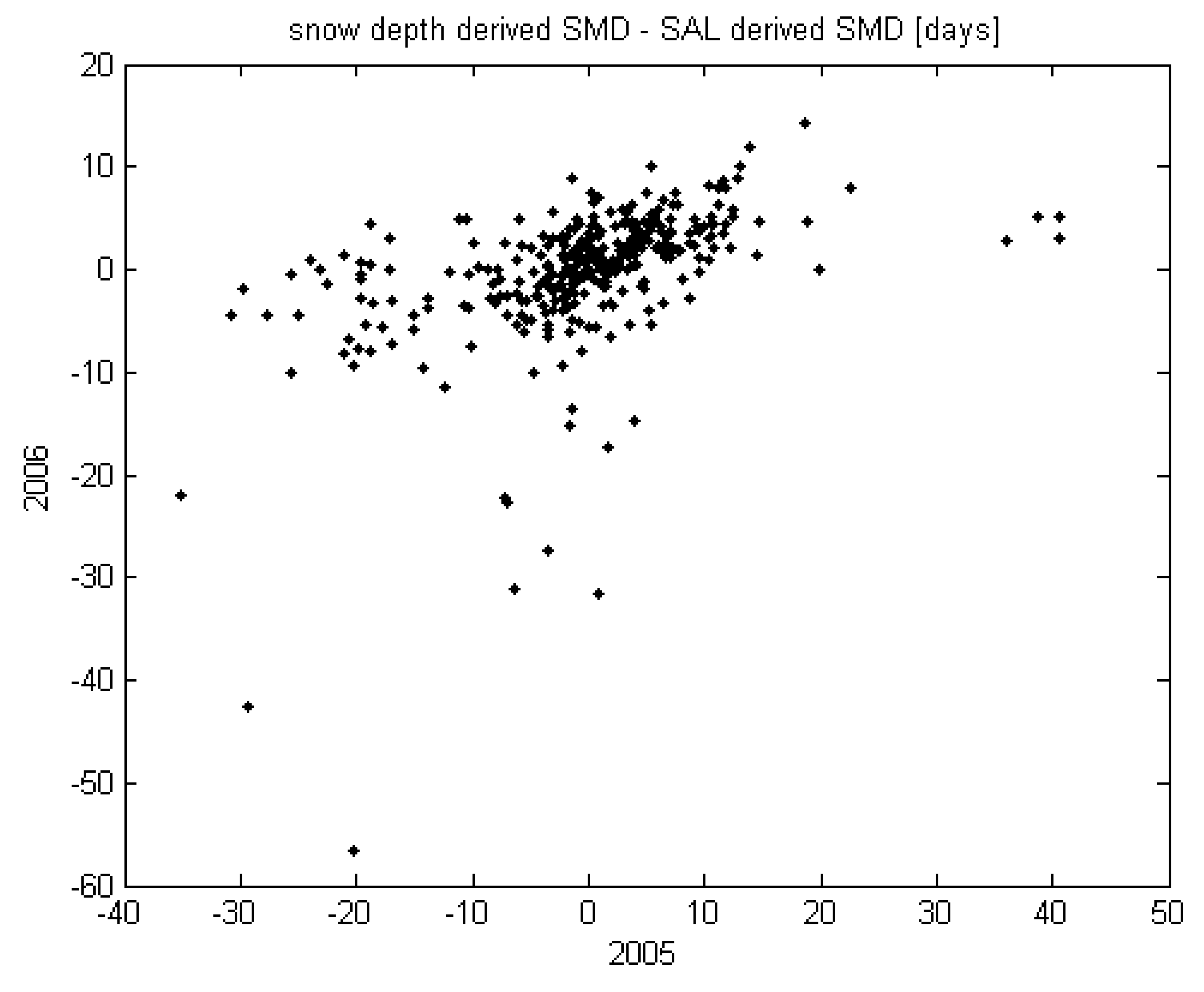
We analyzed the difference between the SMD derived from snow depth measurements and that from the SAL product. First we looked to see whether there is any correlation between the SMD errors in the two different years. Even though there does seem to be slight positive correlation between the errors (
Figure 4), this correlation was not statistically significant. We also investigated whether the error in the SMD correlates with land-use fractions around the surface measurements stations. For this we used the CORINE land-use classification at a 25 × 25 m resolution. We calculated the land-use fractions around the snow depth measurement sites and then correlated these fractions with the difference between the snow depth and the SAL-derived SMD. Out of the 43 land-use classes used for the analysis, six had a correlation coefficient with an absolute value above 0.2. These are listed in
Table 1.
Figure 4.
The difference between snow-depth-derived SMD and SAL-derived SMD at Finnish weather stations in the year 2005 against that in the year 2006.
Figure 4.
The difference between snow-depth-derived SMD and SAL-derived SMD at Finnish weather stations in the year 2005 against that in the year 2006.
Table 1.
Correlation between SMD error ( = snow depth – SAL) and fraction of land-use class around the measurement site.
Table 1.
Correlation between SMD error ( = snow depth – SAL) and fraction of land-use class around the measurement site.
| Land use class | r |
|---|
| Agricultural fields | 0.29 |
| Heath and shrub land | −0.26 |
| Lakes | −0.25 |
| Broadleaved forest on mineral soils | −0.24 |
| Upland soils with sparse vegetation | −0.24 |
| Natural meadows | −0.23 |
The agricultural field is the only land use class which has a positive correlation with the SMD error, whereas others have negative correlations. In a grid square with a high fraction of a land-use class with a negative correlation the SMD derived from satellite data tends to be later than the one derived using snow depth measurement. This can be easily explained for the lake class, as generally lakes melt later than the surrounding land is snow free. Snow depth measurements are always conducted on land, whereas in those areas with a high fraction of lakes, the remotely-sensed albedo is heavily influenced by the lake surfaces. Most of the other land-use types with a negative correlation with SMD error occur in northern highlands. As the surface measurement stations in these regions tend to be situated in valleys, the remotely-sensed SMD, which is influenced by the snow lingering on higher ground, yields later dates. However, due to the limited data set these results are not conclusive.
One source of systematic difference between the satellite and ground-based SMD values is the representativity of the land-use class of the ground measurement stations, which are typically in open areas, whereas 88% of the satellite pixels in Finland were forest-dominated. As in general the snow melts earlier in open areas than in forests, the satellite based SMDs should more often be overestimated than underestimated. This is indeed seen in
Figure 3. However, the opposite behaviour is also possible in cases where the satellite pixel is dominated by open land cover classes but the ground measurement site is shaded by trees, which is sometimes the case, when the measurement site is located in a courtyard edged with trees.
In the area of Russia there are areas with suspiciously early snow melt dates. In order to have a closer look, a time series of satellite-based albedo from this area was studied (data not shown). No high albedo values, typical of snow-covered areas, were observed in these areas during the winter. As the areas just north and south do show high albedo values, it is likely that the satellite-based albedo values from these areas do not represent the true surface albedo. It may be that the low observation angle and small number of cloud free-images available for the area, together with dense coniferous forest cover, leads to this kind of anomalous behaviour.
When using the threshold values derived using the albedo data from summer 2005 to derive the snow melt days for 2006, the result looks very similar to that shown in
Figure 2B (map not shown). In 50% of the cases the difference between the SMD obtained by this method and the surface observations was below 2.8 days, and in 90% of the cases below 7.7 days (graph not shown). For comparison, the same values for the 2006 data with the threshold derived from the same year were 2.8 and 7.8 days, respectively. As the summer time albedo of a 15 × 15 km area usually changes very little between two successive summers, this result is not a surprise. Only in the case of a drastic large-scale change in land use can such a large change in the albedo occur. It can be assumed that the threshold albedo value could be derived using even older data. However, as the available SAL data was limited to the years 2005 and 2006 (2007 being corrupted at the time of writing, while for 2008 a different cloud mask was used) we cannot say how quickly the error in the SMD due to an outdated threshold value would increase.
Aurela
et al., [
1] showed that the CO
2 balance of a subarctic mire ecosystem at Kaamanen, Northern Finland, depended linearly on the timing of snow melt during their 6-year measurement period 1997–2002 (CO
2 balance = SMD × 2.05 [g C m
−2 yr
−1 DOY
−1] − 298.73 [g C m
−2 yr
−1]). We estimated the uncertainty and error that would be introduced into the CO
2 balance by the uncertainty and error in the SAL-based SMD, were we to use the linear dependence to calculate the annual CO
2 balance of this mire. If we use the slope between the SMD and CO
2 balance presented by Aurela
et al., [
1], we see that in 50% of the cases the use of an SAL-based SMD would lead to an uncertainty of 7 g C m
−2 yr
−1 or less for this site. This is 15% of the range of the CO
2 balances (−52 to −4 g C m
−2 yr
−1) observed from 1997 to 2002. What is even more encouraging is the minimal bias in the SMD estimates, which would lead to a systematic error of only 1 g C m
−2 yr
−1.
Currently only two years of the surface albedo product are available at Climate-SAF. For those years, 2005 and 2006, we can compare the annual CO
2 balances of the Kaamanen mire, calculated using the SMD determined from a remotely-sensed surface albedo and the response curve given by Aurela
et al., [
1], to that measured by the eddy covariance technique as described by Aurela
et al., [
1]. In the year 2005, the snow melt at Kaamanen, according to the remotely-sensed surface albedo was May 23rd (DOY 143) and in 2006 May 20th (DOY 140). According to the above-mentioned linear response function, this would lead to CO
2 balances of -5.6 g C m
−2 yr
−1 (2005) and −11.7 g C m
−2 yr
−1 (2006). In contrast, the eddy covariance flux measurements of the annual CO
2 balance of Kaamanen mire were −25 g C m
−2 yr
−1 in 2005 and −40 g C m
−2 yr
−1 in 2006.
Figure 5.
Time series of albedo at the Kaamanen mire measured locally (black solid line) and remotely (circles) in 2006. The error bars mark the periods from which the remotely- measured albedo are determined.
Figure 5.
Time series of albedo at the Kaamanen mire measured locally (black solid line) and remotely (circles) in 2006. The error bars mark the periods from which the remotely- measured albedo are determined.
The snow melt day based on surface observations was May 23rd (DOY 143) in 2005 and May 3rd (DOY 123) in 2006. Thus in 2005 the snow melt day based on remote sensing was the same as that based on surface observation, and the mismatch in the CO
2 balances in this year is not due to the error in the determination of the snow melt. In 2006 the difference in the snow melt based on remote sensing and that based on surface observation is large, 17 days. Based on the surface observations, the snow had melted by May 3rd but later new snow fell, and the ground was snow covered on May 13th–15th (DOY 133–135,
Figure 5). There is a missing week in the remotely-sensed surface albedo data and the data closest to May 3rd are centered at DOY 116 and DOY 137. Thus, it may well be that the actual snow melt is not captured by the method based on the remotely-sensed albedo, as this product was crucially missing at that time, probably due to cloud cover. The later snow cover is then interpreted as a continuation of the winter snow cover.
It is obvious that we cannot draw conclusions on the applicability of the method described in this paper by this very limited comparison. Longer time series of SAL-derived SMD data at mire sites with measurements of annual CO2 balances are needed to assess the applicability of the method. We also need to study how well in general the carbon balances of northern mire and heath ecosystems follow the timing of snow melt. If this is generally true, we need to determine the SMD—CO2-balance response curves for other sites.


