Evaluating the Effects of Environmental Changes on the Gross Primary Production of Italian Forests

Abstract
:1. Introduction
2. Study Area
3. Study Data

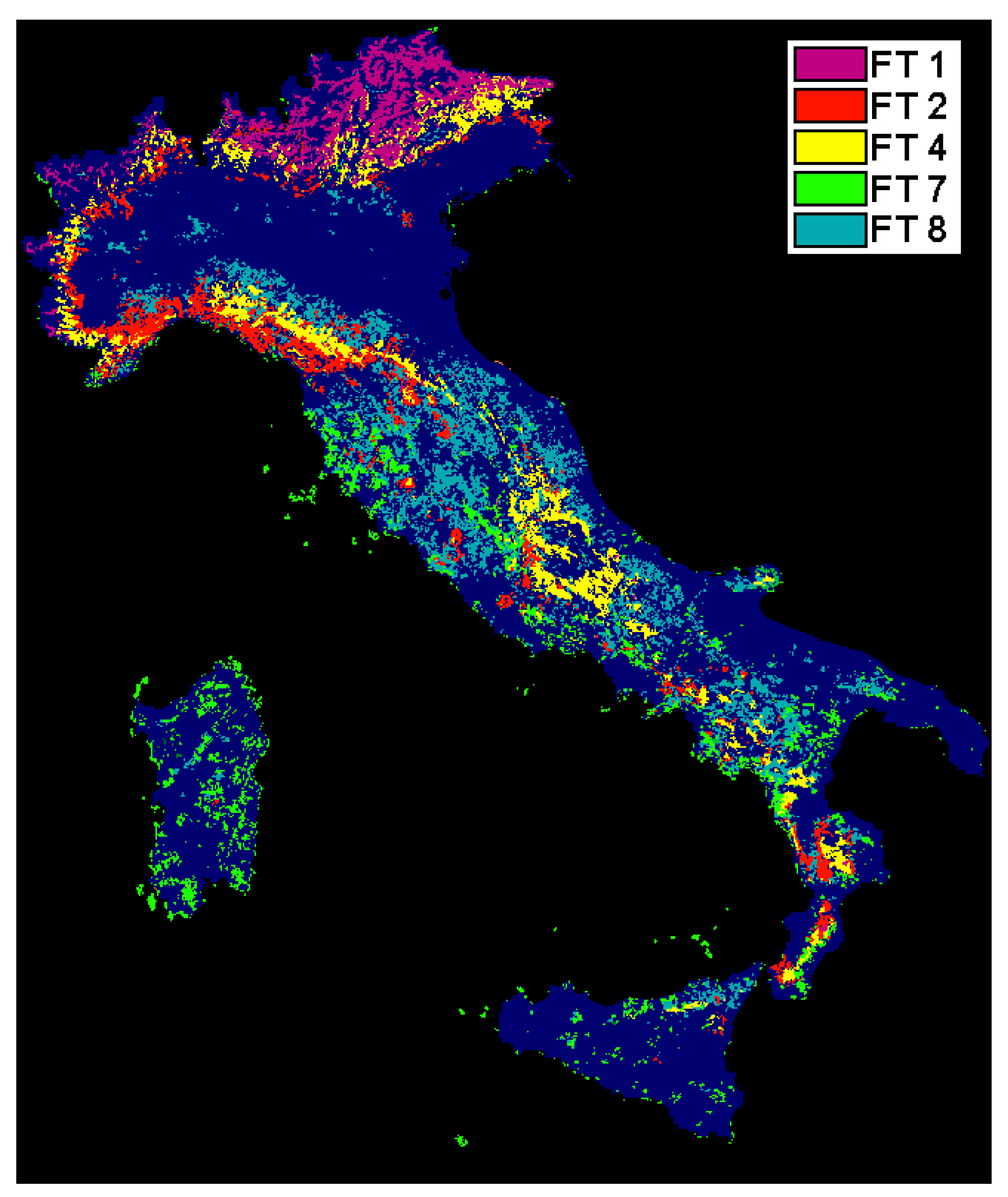
| Index | Forest type | BIOME-BGC type | Area (km2) | Mean altitude (Low/High altitudinal belt) | Mean annual C-Fix GPP (g C/m2/y) |
|---|---|---|---|---|---|
| FT 1 | White fir / Norway spruce | Evergreen needleleaf | 7,742 | 1,424 m asl.(H) | 997 |
| FT 2 | Chestnut | Deciduous broadleaf | 8,437 | 691 m asl.(L) | 1,442 |
| FT 4 | Beech | Deciduous broadleaf | 11,602 | 1,256 m asl.(H) | 1,141 |
| FT 7 | Holm oak | Evergreen broadleaf | 7,025 | 516 m asl.(L) | 1,489 |
| FT 8 | Deciduous oaks | Deciduous broadleaf | 21,347 | 651 m asl.(L) | 1,444 |
4. Methodology
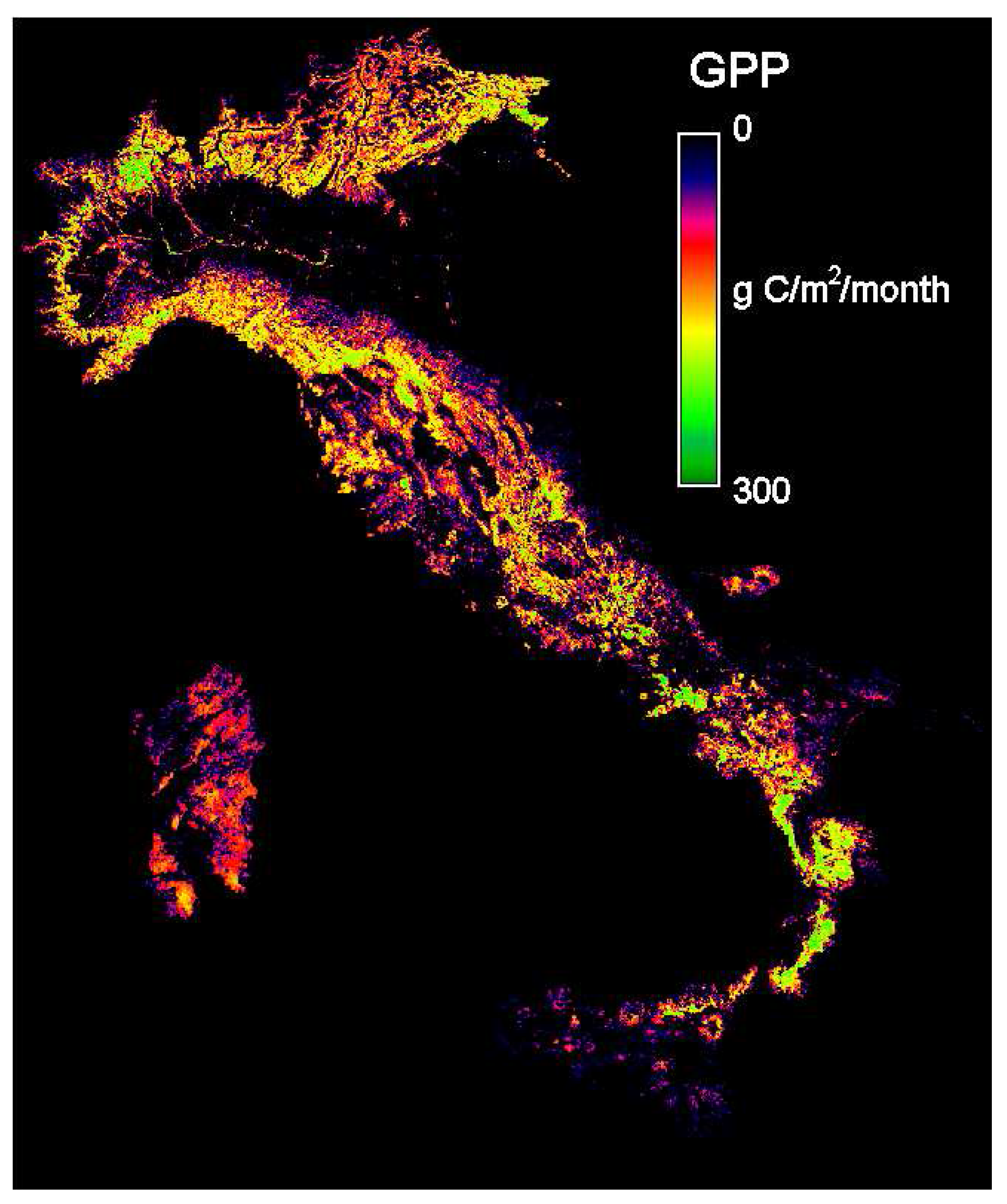
4.1. Application of C-Fix to Present Environmental Conditions
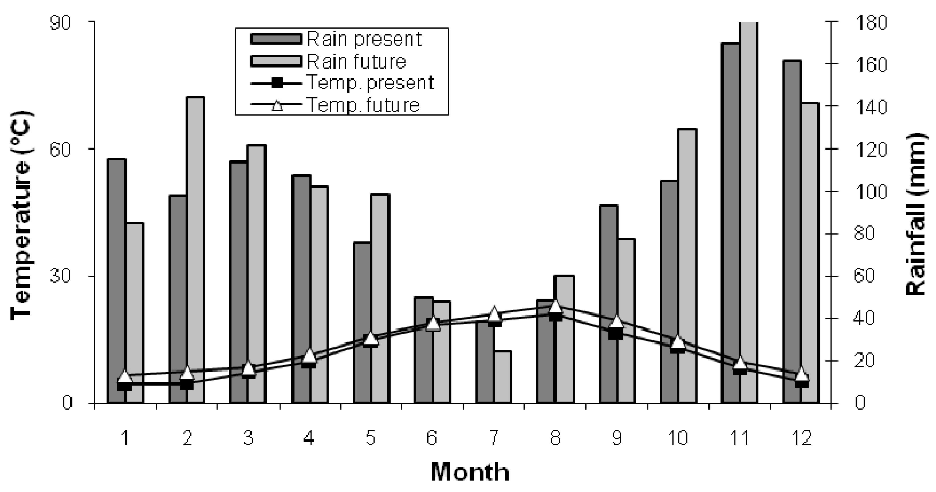
4.2. Simulation of Future Environmental Scenarios
4.3. Evaluation of Future GPP
5. Results

| Forest type | OBSERVED | FUTURE | ||
|---|---|---|---|---|
| Temperature (°C) | Rainfall (mm) | Temperature (°C) | Rainfall (mm) | |
| FT 1 | 6.0 | 1,463.7 | 8.1 | 1,582.1 |
| FT 2 | 11.1 | 1,537.8 | 12.8 | 1,696.9 |
| FT 4 | 7.6 | 1,983.8 | 9.4 | 2,092.6 |
| FT 7 | 13.3 | 1,011.3 | 15.1 | 1,043.0 |
| FT 8 | 11.9 | 1,177.7 | 13.6 | 1,221.1 |

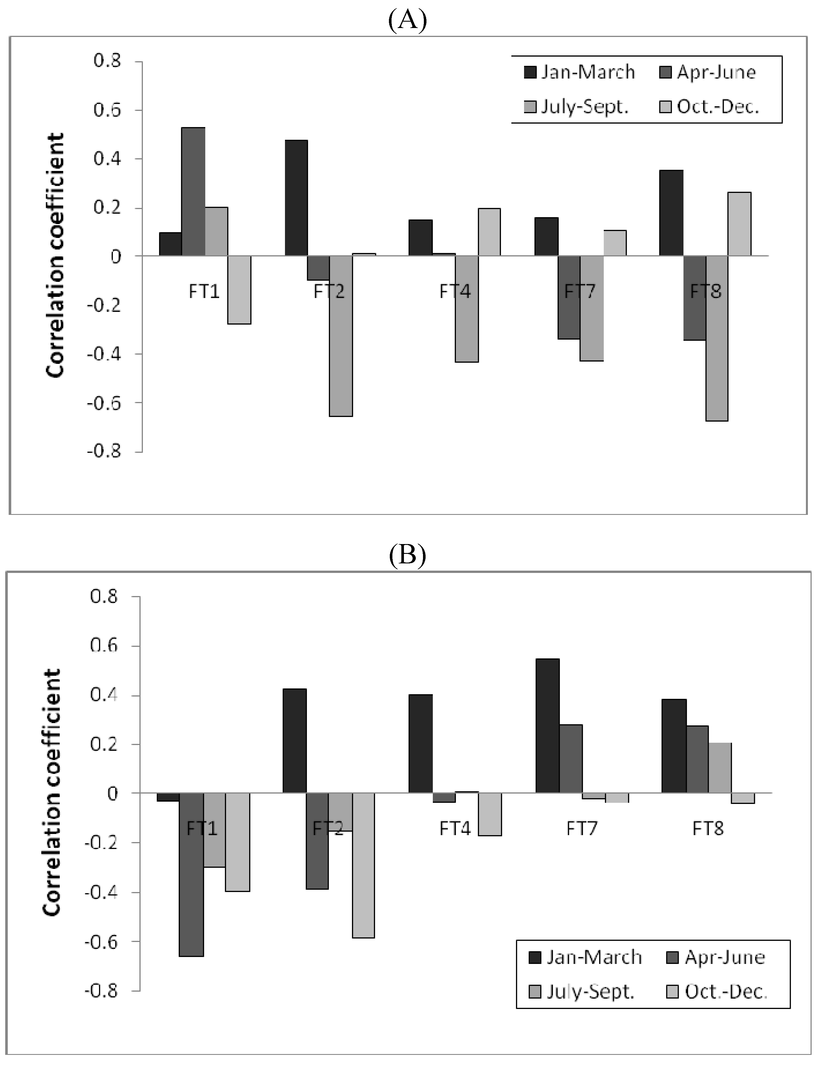
| Temperature | Rainfall | |||||||
|---|---|---|---|---|---|---|---|---|
| r2 | Winter | Spring | Summer | Winter | Spring | Summer | Offset | |
| FT1 | 0.718 | 4.433 | 41.139 | −1.898 | 0.147 | −0.323 | 0.065 | 666.87 |
| FT2 | 0.876 | −11.317 | 46.918 | −98.756 | 0.072 | −0.289 | −0.271 | 2,783.09 |
| FT4 | 0.521 | −10.656 | 47.212 | −44.719 | 0.153 | 0.033 | −0.092 | 1,240.69 |
| FT7 | 0.563 | −2.610 | 20.898 | −37.422 | 0.671 | 0.500 | 0.329 | 1,633.60 |
| FT8 | 0.607 | 5.385 | 23.150 | −50.240 | 0.315 | 0.238 | 0.221 | 1,840.39 |
6. Discussion and Conclusions
Acknowledgements
References
- Waring, H.R.; Running, S.W. Forest ecosystems. In Analysis at Multiples Scales, 3rd ed.; Academic Press: San Diego, CA, USA, 2007. [Google Scholar]
- Hagedorn, F.; Maurer, S.; Egli, P.; Blaser, P.; Bucher, J.B.; Siegwolf, R. Carbon sequestration in forest soils: effects of soil type, atmospheric CO2 enrichment, and N deposition. Europ. J. Soil Scie. 2001, 52, 619–628. [Google Scholar] [CrossRef]
- Pachauri, R.K.; Reisinger, A. (Eds.) Climate change 2007; IPPC Forth Assessment Report; IPCC: Geneva, Switzerland, 2007; p. 104.
- Schlesinger, W.H. Biogeochemestry: an analysis of global change, 2nd ed.; Academic Press: San Diego, CA, USA, 1997. [Google Scholar]
- Field, C.B.; Randerson, J.T.; Malmstrom, C.M. Global net primary production: combining ecology and remote sensing. Remote Sens. Environ. 1995, 51, 74–88. [Google Scholar] [CrossRef]
- Norby, R.J.; Hanson, P.J.; O'Neill, E.G.; Tschaplinski, T.J.; Weltzin, J.F.; Hansen, R.A.; Cheng, W.; Wullschleger, S.D.; Gunderson, C.A.; Edwards, N.T.; Johnson, D.W. Net Primary Productivity of a CO2-Enriched Deciduous Forest and the Implications for Carbon Storage. Ecol. Appl. 2002, 12, 1261–1266. [Google Scholar] [CrossRef]
- Schlesinger, W.H.; Lichter, J. Limited carbon storage in soil and litter of experimental forest plots under increased atmospheric CO2. Nature 2001, 411, 466–469. [Google Scholar] [CrossRef] [PubMed]
- Beerling, D.J. Long-term responses of boreal vegetation to global change: an experimental and modelling investigation. Glob. Change Biol. 1999, 5, 55–74. [Google Scholar] [CrossRef]
- Gielen, B.; Calfapietra, C.; Lukac, M.; Wittig, V.E.; De Angelis, P.; Janssen, I.A.; Moscatelli, M.C.; Grego, S.; Cotrufo, M. F.; Godbold, D.L.; Hoosbeek, M.R.; Long, S.P.; Miglietta, F.; Polle, A.; Bernacchi, C.J.; Davey, P.A.; Ceulemans, R.; Scarascia-Mugnozza, G.E. Net carbon storage in a poplar plantation (POPFACE) after three years of free-air CO2 enrichment. Tree Physiol. 2005, 25, 1399–1408. [Google Scholar] [CrossRef] [PubMed]
- Melillo, J.M.; Steudler, P.A.; Aber, J.D. Soil warming and carbon cycle feedbacks to the climate system. Science 2002, 298, 2173–2175. [Google Scholar] [CrossRef] [PubMed]
- Bronson, D.R.; Gower, S.T.; Tanner, M.; Linder, S.; Van Herk, I. Response of soil surface CO2 flux in a boreal forest to ecosystem warming. Glob. Change Biol. 2008, 14, 856–867. [Google Scholar] [CrossRef]
- Sabatè, S.; Gracia, C.A.; Sanchez, A. Likely effects of climate change on growth of Quercus ilex, Pinus halepensis, Pinus pinaster, Pinus sylvestris and Fagus sylvatica forests in the Mediterranean region. For. Ecol. Manag. 2002, 162, 23–37. [Google Scholar] [CrossRef]
- Osborne, C.P.; Mitchell, P.L.; Sheehy, J.E.; Woodward, F.I. Modelling the recent historical impacts of atmospheric CO2 and climate change on Mediterranean vegetation. Glob. Change Biol. 2000, 6, 445–458. [Google Scholar] [CrossRef]
- Corona, P.; Macrì, A.; Marchetti, M. Boschi e foreste in Italia secondo le più recenti fonti informative. L’Italia Forestale e Montana 2004, 2, 119–136. [Google Scholar]
- Blasi, C.; Chirici, G.; Corona, P.; Marchetti, M.; Maselli, F.; Puletti, N. Spazializzazione di dati climatici a livello nazionale tramite modelli regressivi localizzati. Forest 2007, 2, 213–221. [Google Scholar]
- Maricchiolo, C.; Sambucini, V.; Pugliese, A.; Blasi, C.; Marchetti, M.; Chirici, G.; Corona, P. La realizzazione in Italia del progetto europeo I&CLC2000: metodologie operative e risultati. In Proceedings, 8th National Conference ASITA Geomatica: Standardizzazione, Interoperabilità e Nuove tecnologie; Roma, Italy, 2004; vol. 1, pp. CXIII–CXXVIII. [Google Scholar]
- Bologna, S.; Chirici, G.; Corona, P.; Marchetti, M.; Pugliese, A.; Munafò, M. Sviluppo e implementazione del IV livello CORINE Land Cover per i territori boscati e ambienti semi-naturali in Italia. In Proceedings, 8th National Conference ASITA Geomatica: Standardizzazione, Interoperabilità e Nuove Tecnologie; Roma, Italy, 2004; vol. 1, pp. 467–472. [Google Scholar]
- Maselli, F.; Barbati, A.; Chiesi, M.; Chirici, G.; Corona, P. Use of remotely sensed and ancillary data for estimating forest gross primary productivity in Italy. Remote Sens. Environ. 2006, 100, 563–575. [Google Scholar] [CrossRef] [Green Version]
- Maisongrande, P.; Duchemin, B.; Dedieu, G. Vegetation/Spot: an operational mission for the Earth monitoring; presentation of new standard products. Inter. J. Remote Sens. 2004, 25, 9–14. [Google Scholar] [CrossRef]
- Veroustraete, F.; Sabbe, H.; Eerens, H. Estimation of carbon mass fluxes over Europe using the C-Fix model and Euroflux data. Remote Sens. Environ. 2002, 83, 376–399. [Google Scholar] [CrossRef]
- Veroustraete, F.; Sabbe, H.; Rasse, D.P.; Bertels, L. Carbon mass fluxes of forests in Belgium determined with low resolution optical sensors. Inter. J. Remote Sens. 2004, 25, 769–792. [Google Scholar]
- Myneni, R.B.; Williams, D.L. On the relationship between FAPAR and NDVI. Remote Sens. Environ. 1994, 49, 200–211. [Google Scholar] [CrossRef]
- Running, S.W.; Nemani, R.R.; Heinsch, F.A.; Zhao, M.; Reeves, M.; Hashimoto, H. A continuous satellite-derived measure of global terrestrial primary production. Bioscience 2004, 54, 547–560. [Google Scholar] [CrossRef]
- Bolle, H.J.; Eckardt, M.; Koslowsky, D.; Maselli, F.; Melia-Miralles, J.; Menenti, M.; Olesen, F.S.; Petkov, L.; Rasool, I.; Van de Griend, A. (Eds.) Mediterranean Land-Surface Processes Assessed from Space; Springer: Berlin, Germany, 2006.
- Maselli, F.; Papale, D.; Puletti, N.; Chirici, G.; Corona, P. Combining remote sensing and ancillary data to monitor the gross productivity of water-limited forest ecosystems. Remote Sens. Environ. 2009, 113, 657–667. [Google Scholar] [CrossRef] [Green Version]
- Heinsch, F.A.; Reeves, M.; Votava, P.; Kang, S.; Milesi, C.; Zhao, M.; Glassy, J.; Jolly, W.M.; Loehman, R.; Bowker, C.F.; Kimball, J.S.; Nemani, R.R.; Running, S.W. User’s Guide GPP and NPP (MOD17A2/A3) Products NASA MODIS Land Algorithm. Version 2.0. 2 December 2003. Available online: http://www.ntsg.umt.edu/modis/ (Accessed on November 5th 2009).
- Chiesi, M.; Fibbi, L.; Genesio, L.; Gioli, B.; Maselli, F.; Magno, R.; Moriondo, M.; Vaccari, F. Testing of a strategy to model the carbon fluxes of Mediterranean forest ecosystems. Ecosystems 2009a, in press. [Google Scholar]
- Thornton, P.E.; Running, S.W.; White, M.A. Generating surfaces of daily meteorological variables over large regions of complex terrain. J. Hydrol. 1997, 190, 214–251. [Google Scholar] [CrossRef]
- Thornton, P.E.; Hasenauer, H.; White, M.A. Simultaneous estimation of daily solar radiation and humidity from observed temperature and precipitation: an application over complex terrain in Austria. Agric. For. Meteorol. 2000, 104, 255–271. [Google Scholar] [CrossRef]
- Mizuta, R.; Oouchi, K.; Yoshimura, H.; Noda, A.; Katayama, K.; Yukimoto, S.; Hosaka, M.; Kusunoki, S.; Kawai, H.; Nakagawa, M. 20km-mesh global climate simulations using JMA-GSM model. J. Meteor. Soc. Japan 2006, 84, 165–185. [Google Scholar] [CrossRef]
- Arnell, N.W.; Hudson, D.A.; Jones, R.G. Climate change scenarios from a regional climate model: Estimating change in runoff in southern Africa. J. Geophys. Res. 2003, 108, 4519. [Google Scholar] [CrossRef]
- Yukimoto, S.; Noda, A.; Kitoh, A.; Hosaka, M.; Yoshimura, H.; Uchiyama, T.; Shibata, K.; Arakawa, O.; Kusunoki, S. The Meteorological Research Institute Coupled GCM, Version 2.3 (MRI-CGCM2.3). Control climate and climate sensitivity. J. Meteor. Soc. Japan 2006, 84, 333–363. [Google Scholar] [CrossRef]
- Anderson, T.W. An Introduction to Multivariate Statistical Analysis; John Wiley & Sons: New York, NY, USA, 1984. [Google Scholar]
- Jung, M.; Verstraete, M.; Gobron, N.; Reichstein, M.; Papale, D.; Bondeau, A.; Robustelli, M.; Pinty, B. Diagnostic assessment of European gross primary production. Glob. Change Biol. 2008, 14, 2349–2364. [Google Scholar] [CrossRef]
- Hay, L.E.; Wilby, R.L.; Leavesley, G.H. A comparison of delta change and downscaled GCM scenarios for three mountainous basins in the United States. J. Am. Water Resour. Assoc. 2000, 36, 387–397. [Google Scholar] [CrossRef]
- Giorgi, F.; Mearns, L.O. Approaches to the simulation of regional climate change: a review. Rev. Geophys 1991, 29, 191–216. [Google Scholar] [CrossRef]
- Moberg, A.; Jones, P.D. Regional climate model simulations of daily maximum and minimum near-surface temperatures across Europe compared with observed station data 1961–1990. Clim. Dyn. 2004, 23, 695–715. [Google Scholar] [CrossRef]
- Jacob, D.; Bärring, L.; Christensen, O.B.; Christensen, J.H.; de Castro, M.; Déqué, M.; Giorgi, F.; Hagemann, S.; Hirschi, M.; Jones, R.; Kjeström, E.; Lenderink, G.; Rockel, B.; Sánchez, E.S.; Schär, C.; Seneviratne, S.I.; Somot, S.; van Ulden, A.; van den Hurk, B. An inter-comparison of regional climate models for Europe: model performance in present-day climate. Clim. Change 2007, 81, 31–52. [Google Scholar] [CrossRef]
- Veroustraete, F.; Patyn, J.; Myneni, R.B. Estimating Net Ecosystem Exchange of carbon using the Normalized Difference Vegetation Index and an ecosystem model. Remote Sens. Environ. 1996, 58, 115–130. [Google Scholar] [CrossRef]
- Law, B.E.; Falge, E.; Gu, L.; Baldocchi, D.D.; Bakwin, P.; Berbigier, P.; Davis, K.; Dolman, A.J.; Falk, M.; Fuentes, J.D.; Goldstein, A.; Granier, A.; Grelle, A.; Hollinger, D.; Janssens, I.A.; Jarvis, P.; Jensen, N.O.; Katul, G.; Mahli, Y.; Matteucci, G.; Meyers, T.; Monson, R.; Munger, W.; Oechel, W.; Olson, R.; Pilegaard, K.; Paw, U.K.T.; Thorgeirsson, H.; Valentini, R.; Verma, S.; Vesala, T.; Wilson, K.; Wofsy, S. Environmental controls over carbon dioxide and water vapor exchange of terrestrial vegetation. Agric. For. Met. 2002, 113, 97–120. [Google Scholar] [CrossRef]
- De La Maza, M.; Lima, M.; Meserve, P.L.; Gutierrez, J.R.; Jaksic, F.M. Primary production dynamics and climate variability: ecological consequences in semiarid Chile. Glob. Change Biol. 2009, 15, 1116–1126. [Google Scholar] [CrossRef]
- Ainsworth, E.A.; Long, S.P. What have we learned from 15 years of free-air CO2 enrichment (FACE)? A meta-analytic review of the responses of photosynthesis, canopy properties and plant production to rising CO2. New Phytol. 2005, 165, 351–372. [Google Scholar] [CrossRef] [PubMed]
- Nowak, R.S.; Ellsworth, D.S.; Smith, S.S. Functional responses of plants to elevated atmospheric CO2 – do photosynthetic and productivity data from FACE experiments support early predictions? New Phytol. 2004, 162, 253–280. [Google Scholar] [CrossRef]
- Jones, M.B.; Clifton Brown, J.; Raschi, A.; Miglietta, F. The effects on Arbutus unedo L. of long-term exposure to elevated CO2. Glob. Change Biol. 1995, 1, 295–302. [Google Scholar] [CrossRef]
- Tognetti, R.; Longobucco, A.; Miglietta, F.; Raschi, A. Transpiration and stomatal behavior of Quercus ilex plants during the summer in a Mediterranean carbon dioxide spring. Plant Cell Environ. 1998, 21, 613–622. [Google Scholar] [CrossRef]
- Hattenschwiler, S.; Korner, C. Does elevated CO2 facilitate naturalization of the non-indigenous Prunus laurocerasus in Swiss temperate forests. Funct. Ecol. 2003, 17, 778–785. [Google Scholar] [CrossRef]
- Chiesi, M.; Moriondo, M.; Maselli, F.; Gardin, L.; Fibbi, L.; Bindi, M.; Running, S.W. Simulation of Mediterranean forest carbon pools under expected environmental scenarios. Can. J. For. Res. 2009b, in press. [Google Scholar] [CrossRef]
- Boisvenue, C.; Running, S.W. Impacts of climate change on natural forest productivity – evidence since the middle of the 20th century. Glob. Change Biol. 2006, 12, 862–882. [Google Scholar] [CrossRef]
- Maselli, F.; Chiesi, M.; Bindi, M. Multi-year simulation of Mediterranean forest transpiration by the integration of NOAA-AVHRR and ancillary data. Inter. J. Remote Sens. 2004, 25, 3929–3941. [Google Scholar] [CrossRef]
© 2009 by the authors; licensee Molecular Diversity Preservation International, Basel, Switzerland. This article is an open-access article distributed under the terms and conditions of the Creative Commons Attribution license (http://creativecommons.org/licenses/by/3.0/).
Share and Cite
Maselli, F.; Moriondo, M.; Chiesi, M.; Chirici, G.; Puletti, N.; Barbati, A.; Corona, P. Evaluating the Effects of Environmental Changes on the Gross Primary Production of Italian Forests. Remote Sens. 2009, 1, 1108-1124. https://doi.org/10.3390/rs1041108
Maselli F, Moriondo M, Chiesi M, Chirici G, Puletti N, Barbati A, Corona P. Evaluating the Effects of Environmental Changes on the Gross Primary Production of Italian Forests. Remote Sensing. 2009; 1(4):1108-1124. https://doi.org/10.3390/rs1041108
Chicago/Turabian StyleMaselli, Fabio, Marco Moriondo, Marta Chiesi, Gherardo Chirici, Nicola Puletti, Anna Barbati, and Piermaria Corona. 2009. "Evaluating the Effects of Environmental Changes on the Gross Primary Production of Italian Forests" Remote Sensing 1, no. 4: 1108-1124. https://doi.org/10.3390/rs1041108