Article

Enhanced Automated Canopy Characterization from Hyperspectral Data by a Novel Two Step Radiative Transfer Model Inversion Approach

1
Institute of Photogrammetry and Remote Sensing, Vienna University of Technology, Gusshausstrasse 27-29, 1040 Vienna, Austria
2
German Aerospace Center, German Remote Sensing Data Center (DFD), 82234 Wessling, Germany
3
Institut National de la Recherche Agronomique—EMMAH UMR1114, Agroparc, 84914 Avignon, France
4
German Aerospace Center, Remote Sensing Technology Institute (IMF), 82234 Wessling, Germany
5
Technische Universität München, Lehrstuhl für Methodik der Fernerkundung, Arcisstrasse 21, 80333 Munich, Germany
*
Author to whom correspondence should be addressed.
Remote Sens. 2009, 1(4), 1139-1170; https://doi.org/10.3390/rs1041139
Submission received: 10 September 2009 / Revised: 2 November 2009 / Accepted: 23 November 2009 / Published: 27 November 2009

Abstract

:
Automated, image based methods for the retrieval of vegetation biophysical and biochemical variables are often hampered by the lack of a priori knowledge about land cover and phenology, which makes the retrieval a highly underdetermined problem. This study addresses this problem by presenting a novel approach, called CRASh, for the concurrent retrieval of leaf area index, leaf chlorophyll content, leaf water content and leaf dry matter content from high resolution solar reflective earth observation data. CRASh, which is based on the inversion of the combined PROSPECT+SAILh radiative transfer model (RTM), explores the benefits of combining semi-empirical and physically based approaches. The approach exploits novel ways to address the underdetermined problem in the context of an automated retrieval from mono-temporal high resolution data. To regularize the inverse problem in the variable domain, RTM inversion is coupled with an automated land cover classification. Model inversion is based on a two step lookup table (LUT) approach: First, a range of possible solutions is selected from a previously calculated LUT based on the analogy between measured and simulated reflectance. The final solution is determined from this subset by minimizing the difference between the variables used to simulate the spectra contained in the reduced LUT and a first guess of the solution. This first guess of the variables is derived from predictive semi-empirical relationships between classical vegetation indices and the single variables. Additional spectral regularization is obtained by the use of hyperspectral data. Results show that estimates obtained with CRASh are significantly more accurate than those obtained with a tested conventional RTM inversion and semi-empirical approach. Accuracies obtained in this study are comparable to the results obtained by various authors for better constrained inversions that assume more a priori information. The completely automated and image-based nature of the approach facilitates its use in operational chains for upcoming high resolution airborne and spaceborne imaging spectrometers.

Graphical Abstract

1. Introduction

In agriculture, remote sensing in the reflective optical domain is often used as a cost-effective method to determine spatial and temporal variations in canopy state variables such as leaf area index (LAI) and leaf chlorophyll content. Such variables are driving variables in models predicting growth and yield, and are foreseen to play a major role in precision farming, which aims at optimizing crop management practices to spatial and temporal variability within fields in order to maximize outputs and profit while minimizing ecological impacts [1,2]. In order to be effective, methods providing such indirect estimates from remote sensing data should be highly accurate [3].
Canopy reflectance is controlled by a large number of factors, including the optical properties of vegetation elements (e.g., leaves, stems, and fruits) and soil, and their arrangement, size, and area share in the vegetation canopy. Moreover, at-sensor radiance is highly dependent on the configuration of viewing and illumination angles as well as on the prevailing atmospheric conditions [4,5].
Remote sensing techniques for estimating vegetation characteristics from reflective optical measurements are either based on statistical-empirical or physical approaches, both having their advantages and disadvantages [6]. Statistical-empirical methods are typically based on a regression function between measured biochemical or biophysical properties and spectral measurements in the form of a vegetation index (VI). A VI is a combination of a limited number of spectral bands, selected and combined in a way that enhances spectral features related to the variable of interest while reducing undesired effects caused by variations in soil reflectance, sun and view geometry, atmospheric composition, and other leaf or canopy properties [6]. Classical VIs such as the NDVI [7] and SAVI [8] have been based on broad spectral bands in the visible and near infrared (NIR) part of the spectrum and are particularly suitable to monitor structural vegetation variables such as LAI and fraction of green cover [9]. With the recent development of hyperspectral sensors, new indices have been developed that exploit the information contained in narrow absorption features and the shape of the spectral curve. Such indices have facilitated more accurate estimations, especially of leaf biochemicals like chlorophyll, water, and cellulose [10,11,12]. VI based approaches are computationally fast, but a fundamental problem is their lack of generality. Since canopy reflectance depends on a complex interaction of internal and external factors that may vary significantly in time and space and from one crop type to another, no universal relationship between a single canopy variable and a spectral signature can be expected to exist [13]. Consequently, to be valid over a wide range of species, canopy conditions, and view/sun configurations, these relationships need to be recalibrated for each specific situation, which is a tedious and costly task [14,15,16]. For this reason, the relationships between VIs and biochemical and physical variables are often established by the use of canopy radiative transfer models (RTMs), which explicitly describe the interactions between solar radiation and the elements constituting the canopy using physical laws. RTMs thus allow to generate a virtually endless number of canopy reflectance spectra for which the input variables are known and illumination and view conditions can be controlled [10,17,18,19]. Regression equations developed using RTMs are therefore often more robust than those based on in situ measurements. They are often referred to as predictive equations or predictive relationships [20].
Pure physical retrieval methods involve the inversion of a RTM. The great advantage of RTM inversion is the fact that all variables influencing top of canopy reflectance can be explicitly accounted for. Various strategies have been proposed for the inversion including numerical optimization methods [21,22,23], look-up table approaches [24,25,26] and artificial neural network methods (e.g., [27,28,29]), which all have their strengths and weaknesses in specific situations [6]. The inversion of canopy RTMs is by nature an ill-posed problem mainly for two reasons [24,25]. On the one hand, several combinations of canopy biophysical and biochemical variables have a mutually compensating effect on canopy reflectance thus leading to very similar remote sensing signals. On the other hand, measurement (e.g., radiometric calibration, georectification, atmospheric correction) and model uncertainties and simplifications (e.g., assumptions on canopy architecture) may induce large inaccuracies in the modelled canopy reflectance [30]. Thus, for one and the same input spectrum a large range of plausible results is usually obtained [21].
To reduce the effect of multiple solutions, regularization is required, which involves either the introduction of additional spectral constraints or the introduction of some a priori information about the expected estimates of the variables. Spectral constraints can be obtained by enclosing neighbourhood information through an object-based approach [28] or by increasing the spectral dimensionality of the observation, either by including multiple view angles [25,31,32], or by increasing the number of spectral bands [33,34]. Although hyperspectral remote sensing systems are known to provide additional information on vegetation vitality in waveband ranges that are not accounted for by most multispectral sensors [35,36], up to date such systems are rarely used on an operational basis for the characterization of agricultural crops. Several sources of a priori information about the variables can be considered for remote sensing applications, including ancillary data measured on site, estimates provided by another sensor, knowledge of the dynamic evolution of the biophysical variables over time [37,38], and knowledge about the typical distribution of the input variables in a particular development stage [24]. Land cover classification schemes help to split the problem into sub-domains for which prior information is attributed separately [39,40]. Nevertheless, land cover classification may introduce problems due to misclassification and attribution errors and lead to artefacts at the limit between classes translating into more chaotic spatial or temporal variation of the solution [41]. Moreover, many of the biomes found at the Earth surface are better characterized by gradual transitions then by a crisp classification.
In order to guarantee timely decision support for crop management strategies, remote sensing based products for agricultural applications should be delivered typically within a few days after data acquisition, which implies the use of automated methods. Therefore, this study explores the possibilities of developing a completely automated and image based RTM inversion approach for the concurrent retrieval of the key crop variables LAI, leaf chlorophyll content, leaf water content, leaf dry matter content, and average leaf angle. The approach, which we call CRASh (Canopy variable Retrieval Approach based on PROSPECT and SAILh) is based on the combined leaf reflectance model PROSPECT [36,42] and the canopy radiative transfer model SAILh [43,44]. Innovation of the approach is not the automated model inversion per se, but the exploitation of novel methods to ensure stable RTM inversions for mono-temporal high resolution data in an operational setting where inclusion of a priori information on the variables is strongly hampered. Whereas operational algorithms for medium to low resolution imagery can rely on more frequent coverage, which facilitates land cover classifications in support of retrievals optimized for specific biomes [13,41], a similar option is not offered for the locally operating high resolution systems. Thus, alternative ways are exploited. To regularize the inverse problem in the variable domain, RTM inversion is coupled with an automated land cover classification and a semi-empirical approach based on vegetation indices and RTM simulations. As suggested by [33,34], hyperspectral data is used to further constrain the range of possible solutions in the spectral domain. Even though the CRASh approach has been developed for the inversion of entire images, in this study we confine validation of the approach to simulated and field measured hyperspectral reflectance spectra. In this way we can focus on the performance of the approach itself while excluding inaccuracies resulting e.g., from co-registration errors or scaling issues. Performance of the approach is analysed in terms of prediction accuracy and bias. Its performance is also discussed with regard to a broadly used conventional RTM inversion approach.

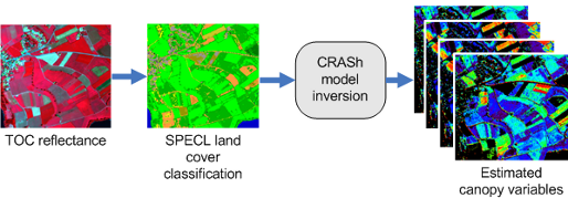
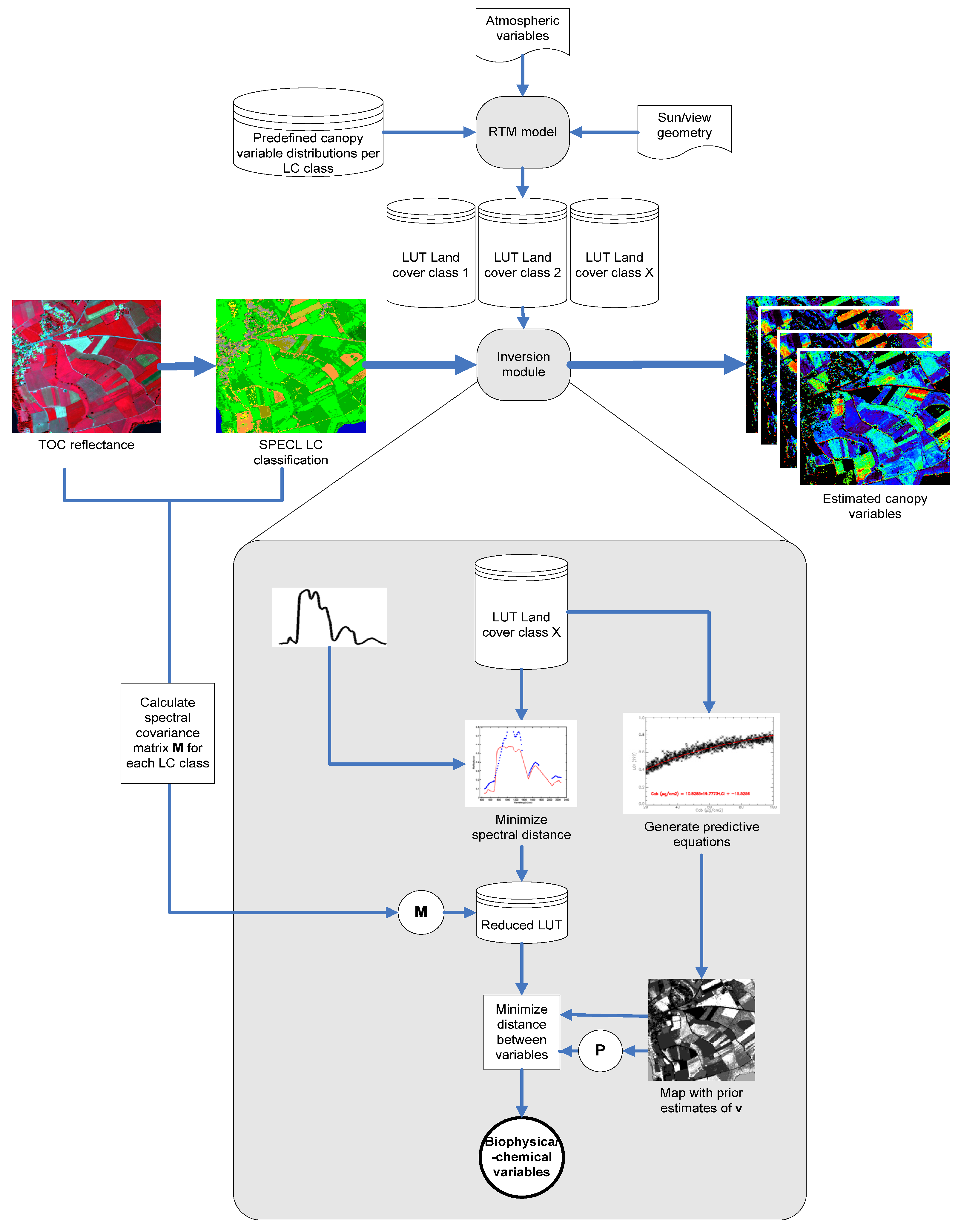
2. The CRASh Radiative Transfer Model Inversion Approach

2.1. Methodological Overview

A schematic overview of the automated CRASh canopy variable retrieval approach is given in Figure 1. The approach is based on the inversion of a canopy radiative transfer model (Section 2.2.). In order to let the inversion take place in a restricted domain of the space of canopy realization, the top of canopy spectra input to the inversion are first submitted to an automated spectral land cover classifier (Section 2.3.). RTM inversion is based on lookup tables (LUTs, Section 2.4.) which are generated for each land cover class separately (Section 2.4.1.). Minimization between the observed reflectance spectrum and the reflectance spectra contained in the LUT takes place first in the radiometric space, and then in the canopy variable space (Section 2.4.2, and Section 2.4.4, respectively). The latter is based on a first estimate of the solution based on predictive regression equations between selected vegetation indices (VI) and each variable input to the radiative transfer model (Section 2.4.3.). The individual components are discussed in more detail in the respective sections. Notice that although the inversion scheme was originally designed for image data, it just as well works with a collection of field spectra.
Figure 1. Overview of CRASh inversion scheme. The upper part shows the general sequence, the grey box shows the inversion approach itself.
Remotesensing 01 01139 g001

2.2. The Radiative Transfer Model

An automated RTM approach for local applications postulates a lack of a priori knowledge about the land cover and the actual status of the vegetation canopy under consideration. This impedes the use of a complex 3-D RTM requiring many input variables, as insufficiently characterizing canopy structure in such a context leads to an increased number of solutions to the ill-posed problem [45]. For this reason, we based our approach on the leaf reflectance model PROSPECT [36,42] and the canopy model SAILh [43,44] which proved their value in a large number of studies and applications (For a comprehensive historic review see [46]). The coupled 1-D turbid medium PROSPECT+SAILh model requires only nine input variables: leaf chlorophyll content Cab (μg cm−2), leaf water content Cw (g cm−2), leaf dry matter content Cdm (g cm−2), leaf brown pigment content Cdm (unitless), leaf mesophyll structure index N, leaf area index LAI (m2 m−2), average leaf angle ALA (°), hot spot variable HS, and soil brightness BS. Canopies demonstrating a complex 3-D structure are not accurately enough characterized with PROSPECT+SAILh, so that application of the model should be confined to canopies obeying the turbid medium assumption in which scattering elements (leaves) are randomly distributed in the canopy volume. This assumption is generally legitimate for most agricultural crops.

2.3. Land Cover Classification

To let the inversion take place in a restricted domain, spectra are first automatically classified with the SPECL spectral land cover classifier [47]. SPECL performs a spectral classification of the reflectance cube based upon template spectra for the Landsat Thematic Mapper (TM) reference wavelengths. The template spectra consist of typical vegetation covers, soil, sand, and water. Rather than explicitly assigning land use or cover type, vegetated surfaces are segregated into various “greenness” classes such as “sparse”, “dark”, “average”, or “bright vegetation” (Figure 2). SPECL uses a framework of decision rules to decide whether a spectrum is assigned to a specific class or not. An overview of the land cover types and decision rules can be found in Table 1.
Figure 2. Template vegetation spectra used in SPECL and typical vegetation types falling into the respective class (in brackets).
Remotesensing 01 01139 g002
The choice to base land cover classification on the Landsat TM band configurations and not on the full hyperspectral reflectance cube is motivated by the fact that the specific absorption features of the land cover types considered in this study are broad enough to allow for a classification based only on this subset of bands. Besides, using Landsat TM template spectra with a limited number of broad wavebands ascertains that spectral classification can be performed independently of the band configuration of the considered hyperspectral sensor. In this way, the spectral classifier does not need to be recalibrated for each sensor which facilitates its use in an operational environment.
Table 1. Decision rules used in SPECL classification, based on reflectance measured at Landsat TM central wave bands: b1 is located at 0.48 μm, b2 at 0.56 μm, b3 at 0.66 μm, b4 at 0.83 μm, b5 at 1.6 μm, b7 at 2.2 μm. aThese expressions are optional and only used if b5 is present. bDecision rule depends on presence of b5. cDecision rule depends on presence of b7.
Class
Snowb4/b3 ≤ 1.3ANDb3 ≥ 0.2ANDb5 ≤ 0.12
Cloudb4 ≥ 0.25AND0.85 ≤ b1/b4 ≤ 1.15ANDb4/b5 ≥ 0.9AND
b5 ≥ 0.2
Bare Soil (bright)b4 ≥ 0.15AND1.3 ≤ b4/b3 ≤ 3.0
Bare Soil (dark)b4 ≥ 0.15AND1.3 ≤ b4/b3 ≤ 3.0ANDb2 ≤ 0.10
Average vegetationb4/b3 ≥ 3.0AND(b1/b3 ≥ 0.8 OR b3 ≤ 0.15)AND0.28 ≤ b4 ≤ 0.4AND
b3 ≤ 0.055
Bright vegetationb4/b3 ≥ 3.0AND(b1/b3 ≥ 0.8 OR b3 ≤ 0.15)ANDb4 ≥ 0.4
Dark vegetationb4/b3 ≥ 3.0AND(b1/b3 ≥ 0.8 OR b3 ≤ 0.15)ANDb3 ≤ 0.08AND
b4 ≤ 0.28
Yellow vegetationb4/b3 ≥ 2.0ANDb2 ≥_b3ANDb3 ≥ 8.0AND
b4/b5 ≥ 1.5 a
Mix vegetation/soil2.0 ≤ b4/b3 ≤ 3.0AND5.0 ≤ b3 ≤ 15.0ANDb4 ≥ 15.0
Asphalt/dark sandb4/b3 ≤ 1.6AND5.0 ≤ b3 ≤ 20.0AND5.0 ≤ b4 ≤ 20.0aAND
5.0 ≤ b5 ≤ 25.0ANDb5/b4 ≥ 0.7a
Sand/bare soil/cloudb4/b3 ≤ 2.0ANDb4 ≥ 0.15ANDb5 ≥ 15.0a
Bright sand/Soil/cloudb4/b3 ≤ 2.0ANDb4 ≥ 0.15AND(b4 ≥ 0.25bOR
b5 ≥ 0.30b)
Dry vegetation / Soil1.7 ≤ b4/b3 ≤ 2.0ANDb4 ≥ 0.25cOR(1.4 ≤ b4/b3 ≤ 2.0AND
b7/b5 ≤ 0.83c)
Sparse vegetation / Soil1.4 ≤ b4/b3 ≤ 1.7ANDb4 ≥ 0.25cOR(1.4 ≤ b4/b3 ≤ 2.0AND
b7/b5 ≤ 0.83ANDb5/b4 ≥ 1.2c)
Turbid Waterb4 ≤ 0.11ANDb5 ≤ 0.05a
Clear Waterb4 ≤ 0.02ANDb5 ≤ 0.02a
Clear water over sandb3 ≥ 0.02ANDb3 ≥ b4 + 0.005ANDb5 ≤ 0.02a

2.4. Lookup Table Inversion

Model inversion is based on a lookup table (LUT) approach. LUT based approaches are a trade-offs between the commonly used, highly flexible, but expensive iterative approaches and neural networks which, once trained, are very fast, but more difficult to adapt to changing local conditions [6,37]. Using a LUT approach involves two steps: i) generation of a synthetic data set, the LUT, and ii) definition of the solution corresponding to the LUT entries that best match a given measurement.
The cost function to minimize between measurement and model may be derived from the maximum a posteriori estimator [24, 48]. The solution is thus found by minimizing:
J ( v ) = ( r r s ) T M 1 ( r r s ) radiometric information + ( v p v ) T P 1 ( v p v ) prior information on variables
where r is the ensemble of radiometric observations (depending on wavebands and observation geometries), rs the radiometric signal simulated with the RTM, v the vector of variables used to simulate rs and vp the vector of expected values of the variables. M and P are the variance-covariance matrices of the measurements and the prior estimates, respectively.
In the case of an automated approach, a priori information about the variables is generally absent or only very vaguely defined. Therefore, we propose a new method for a definition of a first a priori estimate (Section 2.4.3.). As we will see, the first estimates obtained by the proposed method partly depend on the radiometric measurement. Thus, it would be incorrect to speak of a priori knowledge in a strict sense and we decided to abandon common theoretical perception where both parts of the cost function are simultaneously explored and weighted according to the respective covariance matrices. Instead we explore radiometric information and information on the variables in two successive steps (Figure 1). The successive exploration of radiometric and a priori information has been successfully implemented by other authors too [37,49].

2.4.1. Lookup table generation

Based on the SPECL land cover classification, PROSPECT+SAILh is used to generate a LUT for every available class, using the atmospheric characteristics, and view/sun configuration during data acquisition. A soil reflectance spectrum corresponding to an average of local measurements is used to characterise background reflectance. Canopy variables in every class are sampled according to an “experimental plan” [27] in which the total range of expected values is subdivided into a fixed number of intervals from which canopy variables are randomly drawn. The range of variation of each variable depends on the land cover class, although some overlap is maintained between adjoining classes to account for misclassifications. As the number of canopy reflectance realizations increases exponentially with the number of free variables, physically based logics were used to keep computation efforts within reasonable limits. The number of sampling intervals per variable for a given land cover class is determined by the sensitivity of canopy reflectance to the variable in question. For example, BS and Cbp (indicating senescence) receive only one interval for dense, vigorous vegetation classes such as dark and bright vegetation, while LAI and Cab ranges for these classes are subdivided into 8 intervals. The LUTs constructed in this way contain between 30,375 and 141,750 entries in total. Distribution laws of each variable and for each class were determined in such a way that the probability density was proportional to the sensitivity of the reflectance to the variable considered. This allowed better sampling of the domains where reflectance is more sensitive to the considered variables. Where appropriate, a transformation of the distribution according to [26] and [24] was applied. A detailed overview of the employed sampling schemes can be found in Appendix I.

2.4.2. Exploiting radiometric information

Since the (co-)variance between measurement errors is very difficult to characterize, this is commonly ignored. Most authors therefore usually minimize for radiometric information by calculating the root-mean-squared-error (RMSE) between simulated spectrum and LUT entry (e.g., [37,50,51]):
J ( r ) = n = 1 N ( R i R L U T i ) 2 n
where Ri and RiLUT are the reflectance of the input spectrum and the LUT reflectance in band i, respectively, and N equals the number of spectral bands. Nevertheless, in our case we can approximate measurement uncertainty by calculating the spectral covariance from all spectra attributed to a specific SPECL land cover class. Thus, for all spectra within a certain land cover class the same covariance matrix is used. This class based covariance is similar to the object based signatures proposed by [28]. If the covariance matrix appears non-invertible, the variance of the wavebands is used instead. Under this assumption, measurement errors are assumed to be uncorrelated between bands and M in Equation 1 becomes a diagonal matrix. It should be noticed however that M only accounts for non-systematic uncertainties, thus ignoring possible biases due to model assumptions and parameterizations. J(r) is calculated for each LUT entry. The 20% of LUT entries with the best radiometric match (i.e., the smallest J(r) values) are considered possible solutions and subjected to minimization in the variable space (Section 2.3.3). The 20% threshold is consistent with what other authors proposed in earlier studies [37,49].

2.4.3. Using predictive equations for a first guess solution

Apart from the variable ranges and statistical distributions used to simulate the LUTs for the respective land cover classes, no further a priori information on variables is available in an automated approach where each input data set is regarded independently. We therefore propose the use of predictive equations based on RTM simulations to obtain a first estimate of the solution. In the current approach, no additional RTM simulations have to be carried out, since a large number of canopy realizations and accompanying variables for each land cover class are already contained in the LUTs. Moreover, canopy realizations have been optimized for the prevailing illumination/observation geometry, atmospheric conditions and local soil background. In order to make the regression function more robust and realistic, approximations for sensor, measurement, and model uncertainties are attributed to the simulated spectra in the LUT on a random Gaussian basis. According to the average specifications of various sensors (e.g., HyMap, MODIS, Landsat TM), the sensor noise level is set to 0.01 (1%) for wavelengths severely affected by water absorption and to 0.003 (0.3%) for the other wavelengths [52]. Measurement and atmospheric uncertainties, mainly resulting from errors in atmospheric correction, are set to 0.01 (1%; in reflectance units) for the blue range, and 0.006 (0.6%; reflectance units) for the rest of the spectrum [53]. Finally, modelling errors are approximated by the relative standard deviation of spectral measurements of a garden cress performed under laboratory conditions [54]. Such a laboratory set-up excludes any disturbing influences of atmosphere, positioning, or view constellation and is therefore representative for variations in the canopy alone. According to the wavelength range these relative errors range between 0.05 (5%; NIR region) and 0.4 (40%; bands severely affected by atmospheric absorption).
The predictive performance of a certain vegetation index depends on the variable to be estimated, and the canopy, atmospheric, soil, and illumination/view conditions at the time of data recording. Therefore, it was decided not to select one specific vegetation index, but to test for every new situation, land cover class, and variable the predictive performance of a wide range of selected VIs. For this purpose, several VIs developed for vegetation analysis are calculated and plotted versus the different canopy variables. The selected VIs and their appearance are listed in Appendix II. They can be roughly subdivided into four different categories: i) Broadband vegetation indices, originally designed to estimate canopy structural variables such as LAI and fractional cover; ii) Chlorophyll indices which are narrow band indices designed to estimate leaf chlorophyll content; iii) Narrow band water indices, designed to estimate plant water content or detect water stress and having one or more bands in spectral regions sensitive to water absorption, and iv) dry matter indices which are sensitive to one or more of the chemicals composing Cdm, such as lignin and cellulose. For a detailed discussion of characteristics and performance the reader is referred to the original publications or to several publications describing and comparing various VIs [10, 18, 55]. In order to find the best predictive equation, both linear and exponential fits are tested for each combination of variable and VI. For each variable and for each land cover class, the VI and regression function providing the highest predictability (in terms of highest coefficient of determination R2 and lowest root mean squared error of the residuals) were selected to compute a first estimate of the solution from the measured spectra.

2.4.4. Minimizing for first guess of the solution and defining the final solution

Minimization between a priori estimates and the variables in the reduced LUT was performed using:
J ( v ) = ( v p v s ) T W P 1 ( v p v s )
where v­p is the vector with the prior estimates of variables that are left free in the inversion. vs is the set of free variables that was used to simulate s in Equation 1. The covariance matrix P accounts for the non-systematic model errors related to the predictive equations themselves and for the random errors in the predicted values resulting from uncertainties in reflectance (e.g., instrument noise and co-registration errors). This matrix is determined individually for each land cover class and calculated from the a priori estimates of all spectra attributed to this class during land cover classification. W is a diagonal matrix containing the weights that different variables receive in the cost function. These weights correspond to the coefficients of determination that were assigned while establishing the predictive regression equations, with high R2 values corresponding to high weights. The coefficients in W are indicative for the quality of the regression model. They represent the systematic errors and are therefore complementary to P. Thus, prior estimates that are based on high correlation regression models are emphasized while those based on poor predictive equations are suppressed.
The smallest 20% of sorted J(v) values is used to select those entries from the reduced LUT that are used for calculating the final solution of variable vj. The latter is done in a way that the set of variables leading to the smallest J(v) receives largest weight:
v j = k = 1 n ( w k v k j )
where N is the number of entries selected from the LUT reduced during variable minimization and vjk the value of variable vj for LUT entry k. The weight wk, attributed to each particular entry selected from the LUT, is defined by:
w k = 1 / J k ( v ) k = 1 n ( 1 / J k ( v )
where Jk(v) is the result of the cost function for LUT entry k. In principle, all variables input to PROSPECT+SAILh (Section 2.2.) are output by CRASh, although not all variables have importance for further applications.

3. Testing Model Performance

The CRASh inversion approach was first tested on synthetic data, which offers the possibility to study its performance for a large range of differing canopy realizations. In this way, the approach can be tested for all variables left free during inversion. Based on a synthetic data set, especially characteristics and trends concerning the inversion approach itself can be identified, since the physical correctness of the RTM does not have to be accounted for. Secondly, the CRASh approach was used to characterize intensively used grasslands in Central Europe from field spectrometer measurements while validating the results with in situ measurements. In this way also the effect of including actual measurement and model uncertainties and biases could be studied, yet under a more limited range of canopy realizations.

3.1. Synthetic Data Sets

Top of canopy hemispherical directional reflectance factors representing a wide range of crop types and growth stages were calculated with PROSPECT+SAILh using the input variables given in Table 2. Cab, Cw, N, LAI, ALA, and BS varied, whereas Cw and Cdm were fixed at a ratio of 1:4, representing a leaf water content of 80%. Cbp, being of little relevance for green crops, was set to a value close to zero while HS was fixed. For background characterization we used a local soil spectrum measured at the Waging-Taching test site (Section 3.2.1.). Canopy reflectance was calculated for the sensor configuration of the HyMap airborne imaging spectrometer. This sensor covers the electromagnetic spectrum between 0.438 and 2.483 μm with a total of 126 contiguous bands having a full-width-half maximum between 11 and 22 nm [52]. View direction was assumed nadir, the solar zenith angle was set to 35°, and the fraction of diffuse radiation was calculated with MODTRAN4 [53] for a typical mid-European atmosphere (rural aerosol type, visibility = 35 km, water vapour column = 2.0 cm). We considered two scenarios: in the first scenario, the PROSPECT+SAILh model used to generate the synthetic data set was considered free of uncertainties and bias; in the second scenario, we attributed realistic errors to the synthetic spectra according to the approximations for sensor, measurement, and model uncertainties outlined in Section 2.4.3. Both synthetic datasets contained a total number of 270 spectra.
Table 2. Parameterization used for the synthetic data set.
Leaf variablesUnitValues
Cabμg·cm230.0, 50.0, 70.0
Cwg·cm20.0280
Cdmg·cm20.0070
Cbp-0.001
N-1.1, 1.7, 2.3
Canopy variables
LAIm2·m20.5, 1.5, 3.0, 4.5, 6.0
ALA°50.0, 57.0, 64.0
HS-0.1
BS-0.7, 1.3
In order to gain insight into the improvements provided by the CRASh inversion scheme, it was compared to a more conventional radiative transfer model inversion scheme based on a single LUT and minimizing only for spectral reflectance using the RMSE (Equation 2). Selection of the final solution is in line with the one proposed in Section 2.4.2. for the CRASh approach, i.e., the 20% of LUT entries with the best radiometric match were used for calculating the final solution of the variables according to the weighting functions presented in Equations 4 and 5. The accuracy of both model inversion approaches were determined by calculating the RMSE and average relative bias between retrieved values and the variable values used for generating the synthetic spectra.
Table 3. Distribution and sampling plan of the input variables used to construct a comprehensive LUT matching all agricultural land cover types.
Leaf variablesUnitDistribution typeMinimumMaximumMeanσ# intervals
Cabμg·cm−2After [26]1100--6
Cwg·cm−2Uniform0.00500.0800--4
Cdmg·cm−2Uniform0.00200.020--4
Cbp-Gaussian01.50.0010.63
N-Gaussian14.51.513
Canopy variables
LAIm2.m−2After [26]09--6
ALA°Gaussian208557205
HS-Gaussian0.00110.10.35
BS-Gaussian0.31.30.80.33
Assuming automated model inversion, no a priori information on land cover or crop status is available. Therefore, the LUT used for the conventional inversion approach should cover all canopy realizations possibly found for agricultural land use and thus span all the LUTs created for the CRASh approach (Appendix I). The resulting comprehensive LUT contains 388,000 entries. Variable ranges and distribution are given in Table 3.

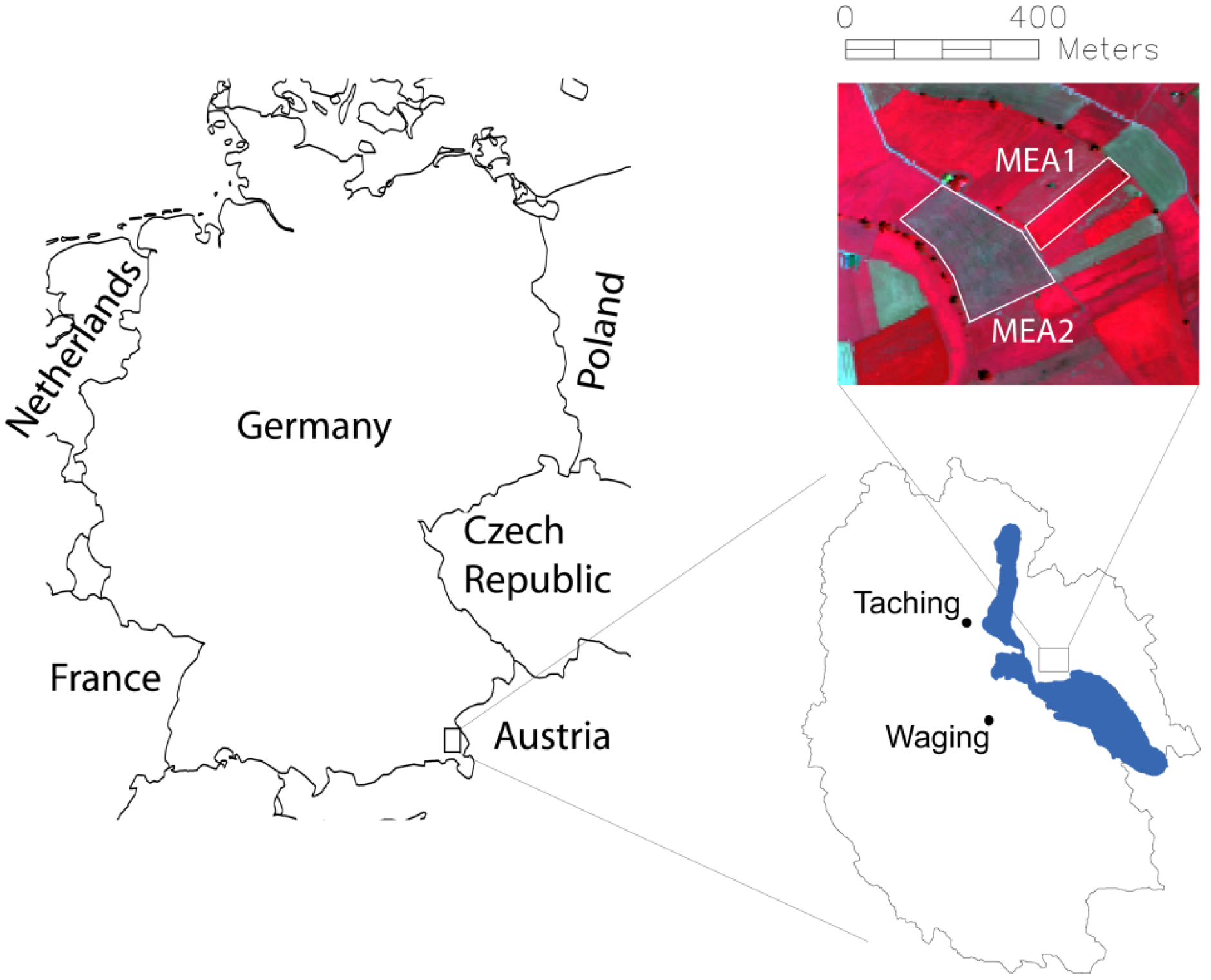
3.2. Inversion of Field Spectra for Temperate Grassland Characterization

3.2.1. Test site

Field spectrometer measurements and validation data were taken in the catchment of Lake Waging-Taching, close to Salzburg in Southeast Germany (Figure 3). Within the study area, two intensively managed meadows were selected for detailed in situ measurements. The two grasslands were sampled by spectroradiometric and biometric field measurements at June 30 and August 4, 2003. At both dates, the first meadow (MEA1) was characterized by a fully developed canopy, while the second meadow (MEA2) had been recently cut and hence contained a considerable amount of dry material. On each field five to seven sample plots, covering an area of 1 × 1 m2, were selected on a stratified basis.
Figure 3. Location of study site within the catchment of Lake Waging-Taching in Southeast Germany. Field boundaries are superimposed on a false colour HyMap hyperspectral image recorded at June 30, 2003 (Red = band 29 (849nm); green = band 15 (646nm); blue = band 9 (555nm).
Remotesensing 01 01139 g003

3.2.2. Biometric sampling

Leaf fresh weight was determined by harvesting the total above ground biomass of the square meter while leaf dry weight was determined after oven-drying the sample at 70 °C for 36 hours. The total amount of water was calculated by the difference between fresh and dry leaf weight. LAI of the entire above ground vegetation of each sample was determined by applying a previously established linear relationship between scanned leaf area and wet biomass (see [56] for details). Cdm and Cw were calculated by dividing leaf dry weight and the total amount of water, respectively, by the LAI [17]. Summary statistics of the measured variable are presented in Table 4.
Table 4. Summary statistics of the measured biophysical and biochemical variables of grassland sample plots.
Measured variablesMinMeanMaxStDev
Cw(g cm-2)0.01880.02310.02640.0024
Cdm(g cm-2)0.00510.00930.01350.0023
LAI(m2 m-2)0.572.396.831.71

3.2.3. Field spectrometer measurements and RTM inversion

Spectral properties of each single sample plot were measured exactly on the location where subsequently the biometric sampling would take place. Per sample plot, ten spectroradiometric measurements were taken from nadir using a portable Fieldspec PRO FR spectrometer (Analytical Spectral Devices, Inc.). The radiance measurements were directly converted into hemispherical directional reflectance factors by taking a Spectralon™ panel as white reference. The single spectra were corrected for the spectral properties of the applied Spectralon panel, deviations of the white reference off the 100 % reflectance line, and spectral jumps between the VNIR and SWIR1 detector [57]. Subsequently, the average reflectance per sample plot was calculated and resampled to the spectral characteristics of the HyMap airborne imaging spectrometer [52]. Bands strongly affected by atmospheric gases and aerosols (i.e., wavelengths < 0.470 μm, between 1.300 and 1.460 μm, between 1.780 and 1.970 μm, and > 2.400 μm) were not considered during inversion, which resulted in a number of 106 bands. Due to technical problems with the spectrometer, only 19 of the initially 23 sample plots could be used for further analysis. Both the spectral RMSE minimization (Equation 2) based on the comprehensive LUT described in Section 3.1. and the CRASh inversion scheme were applied to these spectra.

4. Results and Discussion

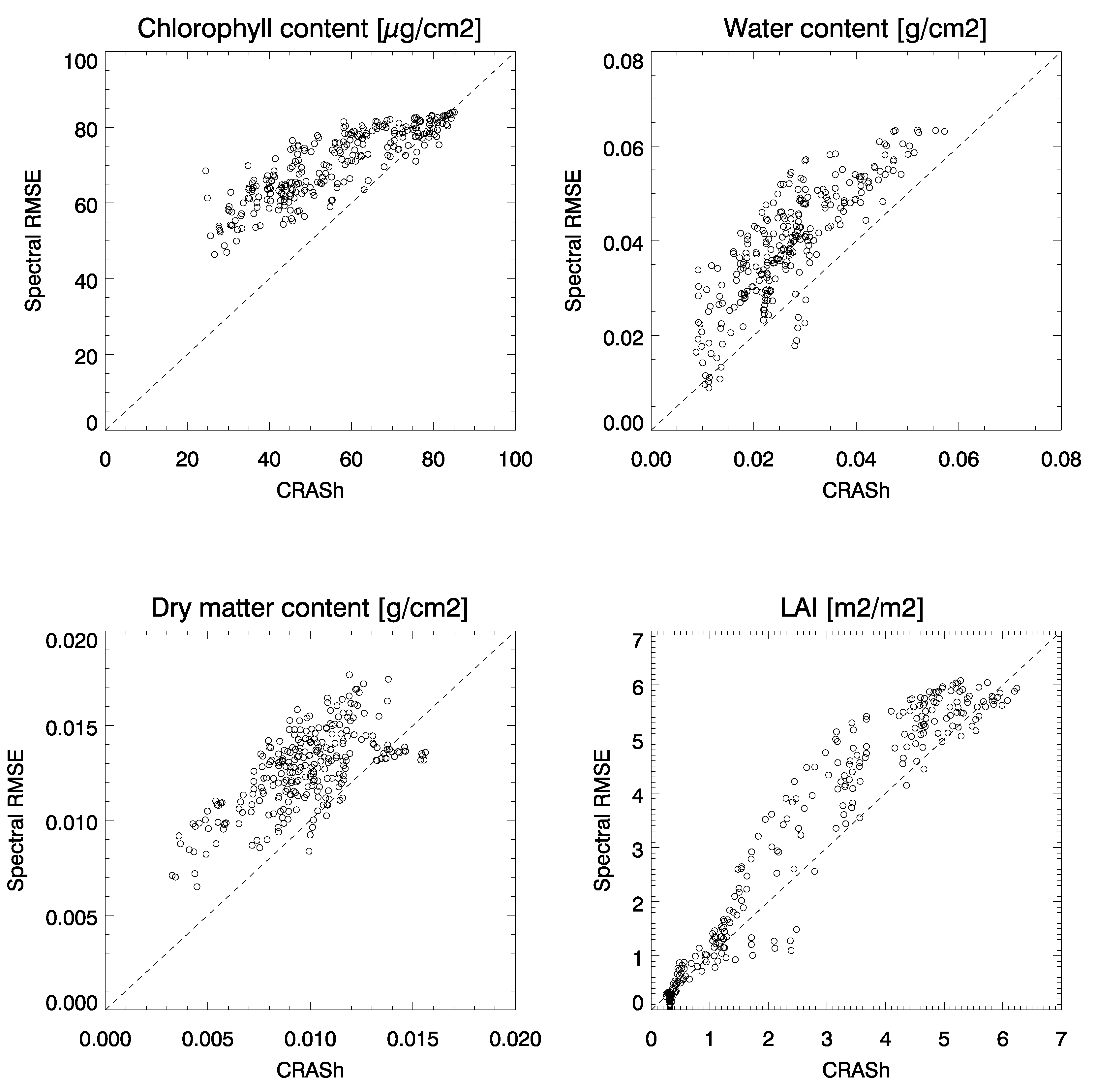
4.1. Synthetic Data Sets

Table 5 shows that the CRASh approach generally provides more accurate estimates than the ones obtained using a comprehensive LUT and the RMSE of reflectance values as cost function (Equation 2). Estimates of Cab, Cw, Cdm, N, and HS are significantly more accurate for the CRASh approach, while accuracies of LAI and ALA retrievals are similar for both approaches. Only estimates of BS are slightly less accurate when using CRASh. Concerning the average relative bias, improvements provided by the CRASh approach for leaf variable estimates and HS are even larger. Only for LAI there is a significant increase in bias compared to the spectral RMSE based inversion. Figure 4 compares the retrievals of the conventional spectral RMSE based approach with those of the CRASh approach for the variables Cab, Cw, Cdm, and LAI.
The plots show the generally higher retrieved values for the conventional RMSE based approach. For the leaf variables this confirms the higher positive biases reported in Table 5. For Cab also the smaller range of solutions for the spectral RMSE based approach compared to CRASh becomes obvious. For the other three considered variables the ranges of estimated values are very similar for both approaches. For LAI the estimates from both approaches coincide well for high and low values, while for intermediate values spectral RMSE based estimates are higher than CRASh based ones. Given the average LAI bias close to zero for the conventional RMSE based approach and the values below zero for the CRASh approach, this might indicate that CRASh slightly underestimates LAI especially in the intermediate range.
Figure 4. Inversion results of CRASh approach versus conventional spectral RMSE based approach.
Remotesensing 01 01139 g004
Adding uncertainty to the synthetic observations appears to have only little influence on the retrieval accuracy, both for the CRASh inversion procedure and the spectral RMSE based inversion scheme. Shifts in relative RMSE and bias values for all cases are within ±5%. These results are indicative for the robustness of the two presented RTM inversion approaches to uncertainties in the input measurements. The large number of spectral bands simultaneously considered during inversion probably has a positive influence in this respect, by levelling the random noise. For model inversion schemes considering a reduced number of bands the effect of adding noise might become more significant.
Table 5. Model inversion results based on synthetic data set for CRASh approach and minimization based on spectral RMSE. All values are given in %. Results for Cbp were not included as these showed values close to infinity due to fixing Cbp to value close to zero.
Perfect model assumptionIncluding uncertainties on model, atmosphere and sensor
CRASh approachSpectral RMSECRASh approachSpectral RMSE
Leaf variablesRMSEBiasRMSEBiasRMSEBiasRMSEBias
Cab29.011.746.940.531.513.646.938.7
Cw36.8-3.658.740.336.0-2.459.537.2
Cdm53.640.086.581.454.636.685.579.1
N33.520.474.470.733.019.574.370.1
Canopy variables
LAI23.7-13.321.2-0.224.3-11.823.92.2
ALA20.5-13.419.6-12.520.6-13.120.2-12.2
HS74.071.0433.1429.678.071.3429.9425.0
BS33.6-16.528.4-11.634.3-17.429.4-12.3
Relative RMSE values obtained with the CRASh approach range between 20.5% and 74.0% for the case were a perfect model is assumed, and between 20.6 and 78.0% when uncertainties on the input spectra are assumed. In both cases these values were obtained for ALA and HS, respectively.

4.2. Field Spectrometer Measurements

Table 6 and Figure 5 show the performance of the spectral RMSE and CRASh in estimating Cw, Cdm and LAI for meadows from spectral field measurements. For the CRASh approach, obtained RMSE values of Cw are comparable to those obtained for the synthetic data set. Biases of Cw retrievals from the spectrometer data are on average more negative than those obtained for the synthetic data sets. Although correlation between measured and estimated Cw is nearly absent, all data pairs, except for one outlier, are concentrated close to the 1:1 line (Figure 5). Accuracies of Cdm retrievals are significantly higher than those obtained for the synthetic data set. This improved accuracy is also expressed by the significantly reduced relative bias, being close to zero. Nevertheless, even though estimates and in situ measurements are located close to the 1:1 line, variation of the differences between measured and estimated differences is still considerable and no clear correlation between measured and estimated values is observed. Also for LAI observed bias improved compared to the synthetic case. However, RMSE is about 10% larger. Of the considered variables only LAI shows a high correlation between measured and estimated values. In contrast to the synthetic data set, intermediate LAI values were slightly overestimated, whereas large LAI values were underestimated (Figure 5).
Table 6. Absolute and relative RMSE between in situ measurements of Cw, Cdm and LAI and estimates obtained from field spectrometer measurements using the CRASh approach.
CRASh approachSpectral RMSE
Absolute RMSERelative RMSERelative BiasAbsolute RMSERelative RMSERelative Bias
Cw0.0080 g·cm-234.5 %-15.3 %0.0052 g·cm-222.4 %2.0%
Cdm0.0030 g·cm-232.8 %-0.1 %0.0035 g·cm-237.4 %28.4 %
LAI0.832 m2·m-234.8 %5.6 %1.355 m2·m-256.7 %38.9 %
Figure 5. In situ measurements of Cw, Cdm and LAI versus estimates obtained from spectral reflectance using the CRASh approach (above) and the spectral RMSE (below). Circles refer to the measurements taken at MEA1, bullets to the measurements taken at MEA2. The dotted line indicates the 1:1 line.
Remotesensing 01 01139 g005
Estimates obtained with the spectral RMSE as a cost function showed clear differences with respect to the simulated data sets. Accuracies of Cw and Cdm clearly improved for the measured data set, whereas the bias encountered for Cdm is still high. Nevertheless, estimation accuracy obtained for Cw, both in terms of RMSE and average bias, is higher than that obtained with CRASh. Regarding LAI, the accuracy and bias obtained for the measured field data are much higher than for the simulated data set and results are clearly inferior to those obtained with CRASh. The scatterplot for spectral RMSE based LAI estimates in the bottom row of Figure 5 shows that especially low measured LAI values are significantly overestimated whereas the estimates for higher measured LAI values are generally in agreement with those obtained using the CRASh approach.

4.3. Land Cover Classification

Classification results of the 19 field spectra considered in this study are found in the second column of Table 7. The classification results generally match the expectancy, i.e., the spectra taken at the recently cut meadow (MEA2) were attributed to SPECL class ”dark vegetation”, “average vegetation” and “mixture of soil and vegetation, whereas spectra taken at the vigorous MEA1 were predominantly attributed to the classes “average vegetation” and “bright vegetation”. Three spectra taken at MEA1 on plots with lower LAI values were attributed to the class “mix vegetation/soil”. Despite the classification of spectra taken at one and the same field into different classes, no inconsistencies in retrieval accuracy resulting from these classification anomalies could be observed. Most likely, this is due to the overlap in parameterization between the classes. Applying CRASh to image data will have to reveal if the chaotic spatial or temporal variation of the solution observed by other authors [41] is overcome with the parameterization used in this study.
Including the SPECL land cover classification attributes leads to improved model inversion due to several reasons: First, it facilitates a more explicit characterization of spectral uncertainties of the measurements and calculating the covariance between different wavebands (Section 2.4.2.). Even though accounting for the covariance theoretically leads to the soundest solution, its influence on the obtained results strongly depends on the band configuration of the sensor and the considered variable [33]. Second, introducing the SPECL land cover classification made it possible to optimize the LUTs for each land cover type and, hence, to let model inversion take place in a restricted variable domain. This in turn reduces the uncertainties related to the individual inversion results. Finally, the LUTs that were calculated separately for each land cover class and illumination/observation geometry allowed for the generation of semi-empirical predictive equations between spectral reflectance and vegetation indices optimized for each specific situation and hence to improved first guesses of the solution. For a detailed discussion on the influence of the single components we refer to [33] and [56].

4.4. A Priori Estimates of the Solution

The quality of the a priori estimates, and thus the final estimate of a certain variable, hinges on the accuracy of the predictive regression equations. As expected, the performance of the predictive regression equations strongly depends on the land cover class and the ensemble of canopy, observation, and illumination characteristics, which, in turn, determines the radiometric effect of each variable (Table 7).
In general, regression functions for Cab, Cw, Cdm, LAI, and ALA perform well with medium to high R2 values and moderate RMS errors. The predictive power of VIs in estimating LAI (expressed by R2 and RMSE) decreases with increasing canopy density. Saturation of spectral reflectance and, hence, an accurate retrieval for LAI values is a well-known phenomenon [22,24]. A reverse trend can be observed for Cw and, to a smaller degree, for Cdm. The trend observed for Cdm is somewhat remarkable since the spectral influence of this leaf constituent is usually masked by leaf water in healthy vegetation [58]. Correlations obtained for ALA are similar for all classes. N, Cbp, HS, and BS show only poor correlations, independent of land cover type. The obtained correlations imply that according to Equation 3 minimization between a priori estimates and variables in the LUT is dominated by Cab, Cw, Cdm, LAI, and ALA while other variables only play a small role.
Table 7. Best performing predictive equations based on simulated spectra in different SPECL classes. The second column shows the results of the SPECL classification applied to the field spectra considered in this study, categorised according to the meadow on which they were taken. For a description of the VI abbreviations see Appendix II. For variables that have a fixed value in the LUT, no predictive equations could be generated.
SPECL classNumber of spectra allocated to class:VariableRegression functionR2RMSE
2MEA1: 0N [–]2.504 − 0.134 · MTCI0.320.61
DarkMEA2: 3Cab [μg·cm−2]16.961 · (127.750REIP1) − 1.0760.7812.6
vegetation Cw [g·cm−2]0.028 + 0.425·LWVI10.660.0097
Cdm [g·cm−2]0.011 − 0.082 · LWVI10.500.0029
Cbp [-]0.932 − 0.027 · TVI0.470.296
LAI [m2·m−2]0.842 · (14.833RDVI) − 1.0760.760.81
ALA [°]70.684 − 40.739 · MTVI10.559.8
HS [–]0.237 · (1.138MCARI1) − 0.1430.090.055
BS [–]0.054 + 0.582 · (1.22GI)0.140.20
3MEA1: 3N [–]−0.032 · (1.467SR705) + 1.8600.220.41
AverageMEA2: 1Cab [μg·cm−2]17.843 · (140.726REIP1) − 564.6210.8611.7
vegetation Cw [g·cm−2]0.016 + 0.202 · LWVI20.670.0118
Cdm [g·cm−2]0.014 − 0.113 · LWVI10.570.0039
Cbp [-]
LAI [m2·m−2]0.024 · (13.069RDVI) − 1.3220.760.94
ALA [°]69.561 − 0.881 · TVI0.529.1
HS [–]0.115 + 0.001 · TVI0.100.080
BS [–]0.403 · (1.201GI) + 0.2630.110.20
4MEA1: 7N [–]−0.097 · (1.324SR705) + 2.0170.280.40
BrightMEA2: 0Cab [μg·cm−2]−42.007 + 178.939·LCI0.8810.8
vegetation Cw [g·cm−2]−0.006 + 0.323 · LWVI20.870.0101
Cdm [g·cm−2]0.016 − 0.111 · LWVI10.580.0047
Cbp [-]
LAI [m2·m−2]1.279 · (8.922RDVI) − 0.6280.481.369
ALA [°]78.459 − 1.201 · TVI0.608.5
HS [–]0.106 + 0.0024 · TVI0.160.082
BS [–]0.054 + 0.582 · (1.22GI)0.070.20
6MEA1: 3N [–]0.904 · (1.618MTVI1) + 0.9690.140.62
Mix soil /MEA2: 2Cab [μg·cm−2]10.035 + 96.910·LCI0.5916.3
vegetation Cw [g·cm−2]0.025 · (39.335LWVI2) − 0.0010.430.0112
Cdm [g·cm−2]0.016 − 0.150 · LWVI10.470.0058
Cbp [-]−0.0004 · (1.217TVI) + 0.2390.470.296
LAI [m2·m−2]1.689 · (2.557TSAVI) − 1.5000.790.48
ALA [°]68.267 − 1.115 · TVI0.559.8
HS [–]9.264e−006 · (1.301TVI) + 0.1610.090.055
BS [–]0.838 + 0.056·GI0.140.20
The best performing VIs selected for each variable were in good agreement with the purpose they were designed for (Table 7). For example, for the canopies and observation/insolation geometry considered in this study Cab was best predicted with the chlorophyll indices LCI and the Red Edge Inflection Point formulation of [59]. Variations in both Cw and Cdm for all classes were best predicted with LWVI1 and LWVI2. The reason that not one of the typical dry matter indices was most suited for predicting Cdm has to be sought in the low sensitivity of spectral reflectance to changes in Cdm in the considered green canopies [58]. Finally, LAI and ALA were best predicted with broad band indices (RDVI, TVI, MTVI1, TSAVI) specifically designed for estimating structural properties. The fact that exclusively narrow band indices performed best in predicting leaf constituents underpins the relevance of hyperspectral data for monitoring crop status.
The question still remains whether the final result is actually improved by minimizing simultaneously for all a priori estimates (Equation 3) instead of directly using the a priori estimates provided by the predictive equations as the final solution. Evidence is provided in Table 8 which shows that the estimates of Cw, Cdm, and LAI as provided by the predictive equations in Table 7 are considerably less accurate than those obtained after minimization in the variable space (cf. Table 6). The reason for the improved estimates based on RTM inversion is twofold. First of all, the predictive equations are based only on a limited number of bands whereas the RTM approach is a full spectrum approach. As a consequence, the semi-empirical approach is more strongly underdetermined leading to more ambiguous solutions. Secondly, the minimization in the variable space offered by CRASh simultaneously accounts for all variables and searches for the most likely solution for all variables together. Moreover, by introducing the covariance between variables, the compensating effect on spectral reflectance of different variables can be accounted for [21,30].
Table 8. Absolute and relative RMSE, and relative bias between in situ measurements of Cw, Cdm and LAI and estimates obtained from field spectrometer measurements using predictive equations.
Absolute RMSERelative RMSERelative Bias
Cw0.0155 g·cm−267.3%51.3%
Cdm0.0033 g·cm−236.0%−1.1%
LAI1.185 m2·m−249.6%16.9%

4.5. Overall Performance

The trends in correlations observed for the predictive equations were partly reflected by the final estimates (Figure 5), showing more accurate LAI retrievals for plots with low measured LAI values and slightly better estimates of Cw and Cdm for plots with high vegetation densities. Similar trends were found for the synthetic data set: The highest accuracies were obtained for those variables that have the largest influence on the TOC spectrum, i.e., Cab, LAI, and ALA. This is conform to what several other studies observed [22,24,60]. Cw and, especially, Cdm were retrieved with less accuracy. The difficulty of accurately retrieving leaf water and leaf dry matter contents from top of canopy green vegetation spectra is explained by the low sensitivity of spectral reflectance to changes in their concentrations and the only small variations usually observed for such canopies. This has already been recognized by many authors [21,22,24,51,60,61]. Remarkably, also N and BS which, according to the predictive equations show only low retrievability, were estimated with reasonable accuracy from the synthetic top of canopy reflectance spectra. The low retrieval accuracies of Cbp and the hotspot parameter HS are in line with the low predictability of this parameter for the considered canopy types (green vegetation) and observation/insolation geometry.
Not all variables output by CRASh have relevance for further applications, e.g., as input to yield models or in the form of stress or drought indicators. Among the variables provided by the CRASh approach, Cab, LAI, and ALA are the most important inputs to process models [62,63]. Based on the synthetic data set with simulated uncertainties and the measured field spectra these variables were retrieved with RMSE values between 20.6 and 34.8%. These accuracies can be considered reasonable given the fully automated nature of the approach and the assumption of total absence of a priori knowledge on land cover and development stage. They are well within the range of accuracies obtained for hyperspectral data in studies where significantly more knowledge on crop type and canopy was a priori available and, hence, the parameterization of model inversion could be better tailored to the prevailing conditions [21,22,24,50]. The regularization proposed by CRASh in most cases provided clear improvements compared to the case where no a priori info at all is available and minimization only takes place in the radiometric domain. Especially variables that are an important input to process models such as Cab and LAI were retrieved with a significantly higher accuracy. Nevertheless, the studied data sets are still too small to draw comprehensive conclusions about the performance of the presented radiative transfer model approach. Specifically, additional spectroradiometric and biophysical measurements performed over different crop types and for a larger range of environmental and phenologic conditions should be included in order to better evaluate model performance under operational conditions.

5. Conclusions and Outlook

In this study we presented the CRASh approach, based on the inversion of the PROSPECT and SAILh radiative transfer models, for automated crop canopy characterization from high resolution hyperspectral data sets. In general, the major limitation of an automated approach is the lack of a priori information on land cover and phenology which strongly hinders the regularization of the ill-posed nature of model inversion. Therefore, we incorporated in CRASh two novel regularization techniques: an automated SPECL land cover classifier [47] and a first guess of the solution based on vegetation indices and radiative transfer model simulations optimized for land cover and view/sun geometry. The use of hyperspectral data provides additional regularization in the spectral domain compared to multispectral systems [33,34].
The results obtained in this study for synthetic data sets and field spectrometer measurements over temperate grassland canopies provided estimates of leaf chlorophyll content and leaf area index that in terms of accuracy are comparable to the results obtained by various authors for better constrained inversions. Even if CRASh does not yet provide the accuracy of 10% required for precision agriculture applications [3], the open structure of the approach allows input from the user side, such as a validated land use map or the definition of plausible phenological properties. Such viable a priori information will most certainly further improve estimation accuracy. Nevertheless, the automated CRASh approach as presented in this study showed the potential of a fully automated, image based retrieval of vital agroecosystem variables, and could be an important contribution towards the incorporation of land surface products in operational chains for upcoming high resolution airborne and spaceborne imaging spectrometers such as APEX [64], ARES [65,66], and EnMap [67].

Acknowledgements

This study was carried out in the framework of the ‘High-Tech Offensive Zukunft Bayern’ project No.290 (‘Pilotprojekt Waging-Tachinger See’) funded by the Bavarian State Ministry of Science, Research, and the Arts. Special thanks go out to Wout Verhoef and Tomi Schneider for their valuable feedback on the topic.

Appendix I Variable sampling plans used for constructing the LUTs for the different SPECL vegetation classes.

Class 2: dark vegetation
Leaf variablesUnitDistribution typeMinimumMaximumMeanσ# intervals
Cabμg cm-2After [26]2090--8
Cwg cm-2Uniform0.01000.0600--5
Cdmg cm-2Uniform0.00350.0150--5
Cbp-Gaussian0.01.50.00.61
N-Gaussian1.03.52.01.03
Canopy variables
LAIm2 m-2After [26]0.56--8
ALA°Gaussian257057203
HS-Gaussian0.0010.20.020.13
BS-Gaussian0.31.10.70.31
Total # of samples :43,200
Class 3: average vegetation
Leaf variablesUnitDistribution typeMinimumMaximumMeanσ# intervals
Cabμg cm-2After [26]20100--8
Cwg cm-2Uniform0.01000.0700--5
Cdmg cm-2Uniform0.00350.0250--5
Cbp-Fixed value0.00.0--1
N-Gaussian1.02.51.630.53
Canopy variables
LAIm2 m-2After [26]1.07.0--8
ALA°Gaussian307057203
HS-Gaussian0.0010.30.050.23
BS-Gaussian0.31.10.70.31
Total # of samples :43,200
Class 4: bright vegetation
Leaf variablesUnitDistribution typeMinimumMaximumMeanσ# intervals
Cabμg cm-2After [26]20100--8
Cwg cm-2Uniform0.01000.0800--5
Cdmg cm-2Uniform0.00500.0250--5
Cbp-Fixed value0.00.0--1
N-Gaussian1.02.51.631.03
Canopy variables
LAIm2 m-2After [26]1.57.0--8
ALA°Gaussian307057203
HS-Gaussian0.0010.30.050.23
BS-Gaussian0.31.10.70.31
Total # of samples :43,200
Class 5: yellow vegetation
Leaf variablesUnitDistribution typeMinimumMaximumMeanσ# intervals
Cabμg cm-2After [26]20100--8
Cwg cm-2Uniform0.01000.0800--5
Cdmg cm-2Uniform0.00500.0250--5
Cbp-Fixed value0.00.0--1
N-Gaussian1.02.51.631.03
Canopy variables
LAIm2 m-2After [26]2.09.0--8
ALA°Gaussian307057203
HS-Gaussian0.0010.30.20.23
BS-Gaussian0.31.10.70.31
Total # of samples :43,200
Class 6: mix of vegetation and soil
Leaf variablesUnitDistribution typeMinimumMaximumMeanσ# intervals
Cabμg cm-2After [26]1080--7
Cwg cm-2Uniform0.00700.0500--5
Cdmg cm-2Uniform0.00200.0250--5
Cbp-Gaussian0.00.50.00.52
N-Gaussian1.03.51.71.03
Canopy variables
LAIm2 m-2After [26]0.23.0--5
ALA°Gaussian306057203
HS-Gaussian0.010.30.20.33
BS-Gaussian0.51.20.90.23
Total # of samples :141,750
Class 12: dry vegetation/soil
Leaf variablesUnitDistribution typeMinimumMaximumMeanσ# intervals
Cabμg cm-2After [26]020--3
Cwg cm-2Uniform0.00100.0100--5
Cdmg cm-2Uniform0.00200.0150--5
Cbp-Gaussian0.01.50.00.63
N-Gaussian1.54.02.21.03
Canopy variables
LAIm2 m-2After [26]0.1.5--5
ALA°Gaussian307057203
HS-Gaussian0.010.80.20.21
BS-Gaussian0.71.31.00.23
Total # of samples :30,375
Class 13: sparse vegetation/soil
Leaf variablesUnitDistribution typeMinimumMaximumMeanσ# intervals
Cabμg cm-2After [26]040--5
Cwg cm-2Uniform0.00500.0300--5
Cdmg cm-2Uniform0.00200.0200--5
Cbp-Gaussian0.00.50.00.52
N-Gaussian1.04.01.71.03
Canopy variables
LAIm2 m-2After [26]0.011.5--5
ALA°Gaussian307057203
HS-Gaussian0.010.80.20.21
BS-Gaussian0.71.31.00.23
Total # of samples :33,750

Appendix II. Vegetation indices used to provide a first estimate of the output result. Rx indicates the reflectance value in band x.

Vegetation indexEquationReference
Broadband vegetation indices / canopy structure indices
Normalized Difference Vegetation Index (NDVI) ( R 850 R 670 ) / ( R 850 + R 670 ) [7]
Ratio Vegetation Index (RVI) R 850 / R 670 [68]
Soil-Adjusted Vegetation Index (SAVI) ( 1 + L ) ( R 850 R 670 ) / ( R 850 + R 670 + L ) [8]
Soil-Adjusted Vegetation Index 2 (SAVI2) R 850 / ( R 670 + a b / b c ) [69]
Modified Soil-Adjusted Vegetation Index (MSAVI) 0.5 ( 2 R 850 + 1 ( 2 R 850 + 1 ) 2 8 ( R 850 R 670 ) ) [70]
Optimized Soil-Adjusted Vegetation Index (OSAVI) ( 1 + 0.16 ) ( R 850 R 670 ) / ( R 850 + R 670 + 0.16 ) [71]
Transformed Soil-Adjusted Vegetation Index (TSAVI) a * ( R 850 a R 670 b ) / ( R 670 + a R 850 a b ) [72]
Adjusted Transformed Soil Adjusted Vegetation Index (ATSAVI) a ( R 850 a R 670 b ) ( a R 850 + R 670 a b + X ( 1 + a 2 ) ) [14]
Renormalized Difference Vegetation Index (RDVI) ( R 850 R 670 ) / ( R 850 + R 670 ) [5]
Triangular Vegetation Index (TVI) ( 60 ( R 750 R 550 ) 100 ( R 670 R 550 ) ) [55]
Modified Triangular Vegetation Index 1 (MTVI1) 1.2 ( 1.2 ( R 800 R 550 ) 2.5 ( R 670 R 550 ) ) [10]
Modified Triangular Vegetation Index 2 (MTVI2) 1.5 ( 1.2 ( R 800 R 550 ) 2.5 ( R 670 R 550 ) ) ( 2 R 800 + 1 ) 2 ( 6 R 800 5 R 670 ) 0.5 [10]
Narrow band chlorophyll indices
Chlorophyll Absorption Reflectance Index (CARI) ( R 701 / R 671 ) | ( a 670 + R 671 + b ) / ( a 2 + 1 ) [73]
Transformed Chlorophyll Absorption Ratio Index (TCARI) 3 [ ( R 700 R 670 ) 0.2 ( R 700 R 550 ) ( R 700 / R 670 ) ] [74]
Modified Chlorophyll Absorption Reflectance Index (MCARI) [ ( R 700 R 670 ) 0.2 ( R 700 R 550 ) ] ( R 700 / R 670 ) [75]
Modified Chlorophyll Absorption Reflectance Index (MCARI1) 1.2 [ 2.5 ( R 800 R 670 ) 2.5 ( R 800 R 550 ) ] [10]
Modified Chlorophyll Absorption Reflectance Index (MCARI2) 1.5 ( 2.5 ( R 800 R 670 ) 1.3 ( R 800 R 550 ) ) ( 2 R 800 + 1 ) 2 ( 6 R 800 5 R 670 ) 0.5 [10]
Simple Ratio at 705 Index (SR705) R 750 / R 705 [76]
Normalized Difference Index (mND705) ( R 750 R 705 ) / ( R 750 + R 705 2 R 440 ) [76]
Greenness Index (GI) R 554 / R 677 [18]
Photochemical Reflectance Index (PRI) ( R 529 R 569 ) / ( R 529 + R 569 ) [77]
Red Edge Inflection Point (REIP1) ( 700 + ( 740 / 700 ) ( R i R 780 ) / ( R 740 + R 701 ) ; R i = R 780 / R 670 [59]
Red Edge Inflection Point (REIP2)Maximum of 1st derivative obtained by Savitzky – Golay filtering[78]
Red Edge Inflection Point (REIP3)Minimum of 2nd derivative obtained by Savitzky – Golay filtering[78]
Red Edge Inflection Point (REIP4)REIP calculation based on lagrangian interpolation.[79]
1st-order Derivative-based Green Vegetation Index (DGVI1)Surface under the curve of the first derivative between 680 and 760 nm[80]
2nd-order Derivative-based Green Vegetation Index (DGVI2)Surface under the curve of the second derivative between 680 and 760 nm[80]
Carter Stress Index 2 (CSI2) R 695 / R 760 [81]
Narrow band water indices
Moisture Stress Index (MSI) R 1600 / R 820 [82]
Leaf Water Vegetation Index 1 (LWVI1) ( R 1094 R 983 ) / ( R 1094 + R 983 ) [11]
Leaf Water Vegetation Index 2 (LWVI2) ( R 1094 R 1205 ) / ( R 1094 + R 1205 ) [11]
Disease Water Stress Index 5 ( R 800 + R 550 ) / ( R 1660 + R 680 ) [83]
Narrow band dry matter indices
Normalized Difference Nitrogen Index (NDNI)
log ( R 1510 ) 1 log ( R 1680 ) 1 log ( R 1510 ) 1 + log ( R 1680 ) 1
[84]
Normalized Difference Lignin Index (NDLI)
log ( R 1094 ) 1 log ( R 1205 ) 1 log ( R 1094 ) 1 + log ( R 1205 ) 1
[84]
Cellulose Absorption Index (CAI)
0.5 ( R 2015 + R 2195 ) R 2106
[12]
Shortwave Infrared Green Vegetation Index (SWIRVI)
37.27 ( R 2210 + R 2090 ) + 26.27 ( R 2208 R 2090 ) 0.57
[85]
L = 0.5 [14]; a = 1.2 [14,55]; b = 0.04 [14]; X=0.08 [14]; β = 1 [86]

References and Notes

  1. Bastiaanssen, W.G.M.; Ali, S. A new crop yield forecasting model based on satellite measurements applied across the Indus Basin, Pakistan. Agr. Ecosyst. Environ. 2003, 94, 321–340. [Google Scholar] [CrossRef]
  2. Moran, M.S.; Inoue, Y.; Barnes, E.M. Opportunities and limitations for image-based remote sensing in precision crop management. Remote Sens. Environ. 1997, 61, 319–346. [Google Scholar] [CrossRef]
  3. Harmoney, K.R.; Moore, K.J.; George, J.R.; Brummer, E.C.; Russell, J.R. Determination of pasture biomass using four indirect methods. Agron. J. 1997, 89, 665–672. [Google Scholar] [CrossRef]
  4. Cierniewski, J.; Verbrugghe, M. Influence of soil surface roughness on soil bidirectional reflectance. Int. J. Remote Sens. 1997, 18, 1277–1288. [Google Scholar] [CrossRef]
  5. Roujean, J.-L.; Bréon, F.-M. Estimating PAR absorbed by vegetation from bidirectional reflectance measurements. Remote Sens. Environ. 1995, 51, 375–384. [Google Scholar] [CrossRef]
  6. Dorigo, W.A.; Zurita-Milla, R.; de Wit, A.J.W.; Brazile, J.; Singh, R.; Schaepman, M.E. A review on reflective remote sensing and data assimilation techniques for enhanced agroecosystem modeling. Int. J. Appl. Earth Obs. Geoinf. 2007, 9, 165–193. [Google Scholar] [CrossRef]
  7. Rouse, J.W.; Haas, R.H.; Schell, J.A.; Deering, J.A. Monitoring vegetation systems in the Great Plains with ERTS. In Proceedings of Third Symposium on Significant Results Obtained with ERTS -1, NASA; Goddard Space Flight Center: Greenbelt, MD, USA, 1973; Volume 1, pp. 309–317, (SEE N74-30705 20-13). [Google Scholar]
  8. Huete, A.R. A soil-adjusted vegetation index (SAVI). Remote Sens. Environ. 1988, 25, 295–309. [Google Scholar] [CrossRef]
  9. Huete, A.R.; Liu, H.Q.; Batchily, K.; van Leeuwen, W. A comparison of vegetation indices over a global set of TM images for EOS-MODIS. Remote Sens. Environ. 1997, 59, 440–451. [Google Scholar]
  10. Haboudane, D.; Miller, J.R.; Pattey, E.; Zarco-Tejada, P.J.; Strachan, I.B. Hyperspectral vegetation indices and novel algorithms for predicting green LAI of crop canopies: Modeling and validation in the context of precision agriculture. Remote Sens. Environ. 2004, 90, 337–352. [Google Scholar] [CrossRef]
  11. Galvão, L.S.; Formaggio, A.R.; Tisot, D.A. Discrimination of sugarcane varieties in Southeastern Brazil with EO-1 Hyperion data. Remote Sens. Environ. 2005, 94, 523–534. [Google Scholar] [CrossRef]
  12. Nagler, P.L.; Inoue, Y.; Glenn, E.P.; Russ, A.L.; Daughtry, C.S.T. Cellulose absorption index (CAI) to quantify mixed soil-plant litter scenes. Remote Sens. Environ. 2003, 87, 310–325. [Google Scholar] [CrossRef]
  13. Houborg, R.; Soegaard, H.; Boegh, E. Combining vegetation index and model inversion methods for the extraction of key vegetation biophysical parameters using Terra and Aqua MODIS reflectance data. Remote Sens. Environ. 2007, 106, 39–58. [Google Scholar] [CrossRef]
  14. Baret, F.; Guyot, G. Potentials and limits of vegetation indices for LAI and APAR assessment. Remote Sens. Environ. 1991, 35, 161–173. [Google Scholar] [CrossRef]
  15. Verrelst, J.; Schaepman, M.E.; Koetz, B.; Kneubühler, M. Angular sensitivity analysis of vegetation indices derived from CHRIS/PROBA data. Remote Sens. Environ. 2008, 112, 2341–2353. [Google Scholar] [CrossRef]
  16. Colombo, R.; Bellingeri, D.; Fasolini, D.; Marino, C.M. Retrieval of leaf area index in different vegetation types using high resolution satellite data. Remote Sens. Environ. 2003, 86, 120–131. [Google Scholar] [CrossRef]
  17. Ceccato, P.; Flasse, S.; Tarantola, S.; Jacquemoud, S.; Grégoire, J.-M. Detecting vegetation leaf water content using reflectance in the optical domain. Remote Sens. Environ. 2001, 77, 22–33. [Google Scholar] [CrossRef]
  18. Zarco-Tejada, P.J.; Berjon, A.; Lopez-Lozano, R.; Miller, J.R.; Martin, P.; Cachorro, V.; Gonzalez, M.R.; de Frutos, A. Assessing vineyard condition with hyperspectral indices: Leaf and canopy reflectance simulation in a row-structured discontinuous canopy. Remote Sens. Environ. 2005, 99, 271–287. [Google Scholar] [CrossRef]
  19. Zarco-Tejada, P.J.; Ustin, S.L. Modeling canopy water content for carbon estimates from MODIS data at land EOS validation sites. In Proceedings of International Geoscience and Remote Sensing Symposium, Sydney, Australia, 2001; Vol. 1, pp. 342–344.
  20. Gastellu-Etchegorry, J.P.; Bruniquel-Pinel, V. A modeling approach to assess the robustness of spectrometric predictive equations for canopy chemistry. Remote Sens. Environ. 2001, 76, 1–15. [Google Scholar] [CrossRef]
  21. Jacquemoud, S.; Baret, F.; Andrieu, B.; Danson, F.M.; Jaggard, K. Extraction of vegetation biophysical parameters by inversion of the PROSPECT + SAIL models on sugar beet canopy reflectance data. Application to TM and AVIRIS sensors. Remote Sens. Environ. 1995, 52, 163–172. [Google Scholar] [CrossRef]
  22. Vohland, M.; Jarmer, T. Estimating structural and biochemical parameters for grassland from spectroradiometer data by radiative transfer modelling (PROSPECT+SAIL). Int. J. Remote Sens. 2008, 29, 191–209. [Google Scholar] [CrossRef]
  23. Lavergne, T.; Kaminski, T.; Pinty, B.; Taberner, M.; Gobron, N.; Verstraete, M.M.; Vossbeck, M.; Widlowski, J.L.; Giering, R. Application to MISR land products of an RPV model inversion package using adjoint and Hessian codes. Remote Sens. Environ. 2007, 107, 362–375. [Google Scholar] [CrossRef]
  24. Combal, B.; Baret, F.; Weiss, M.; Trubuil, A.; Macé, D.; Pragnère, A.; Myneni, R.; Knyazikhin, Y.; Wang, L. Retrieval of canopy biophysical variables from bidirectional reflectance using prior information to solve the ill-posed inverse problem. Remote Sens. Environ. 2002, 84, 1–15. [Google Scholar] [CrossRef]
  25. Knyazikhin, Y.; Martonchik, J.V.; Diner, D.J.; Myneni, R.B.; Verstraete, M.; Pinty, B.; Gobron, N. Estimation of vegetation canopy leaf area index and fraction of absorbed photosynthetically active radiation from atmosphere-corrected MISR data. J. Geophys. Res D Atmos. 1998, 103, 32239–32256. [Google Scholar] [CrossRef]
  26. Weiss, M.; Baret, F.; Myneni, R.B.; Pragnère, A.; Knyazikhin, Y. Investigation of a Model Inversion Technique to Estimate Canopy Biophysical Variables from Spectral and Directional Reflectance Data. Agronomie 2000, 20, 3–22. [Google Scholar] [CrossRef]
  27. Bacour, C.; Baret, F.; Beal, D.; Weiss, M.; Pavageau, K. Neural network estimation of LAI, fAPAR, fCover and LAIxCab, from top of canopy MERIS reflectance data: Principles and validation. Remote Sens. Environ. 2006, 105, 313–325. [Google Scholar] [CrossRef]
  28. Atzberger, C. Object-based retrieval of biophysical canopy variables using artificial neural nets and radiative transfer models. Remote Sens. Environ. 2004, 93, 53–67. [Google Scholar] [CrossRef]
  29. Baret, F.; Hagolle, O.; Geiger, B.; Bicheron, P.; Miras, B.; Huc, M.; Berthelot, B.; Niño, F.; Weiss, M.; Samain, O.; Roujean, J.L.; Leroy, M. LAI, fAPAR and fCover CYCLOPES global products derived from VEGETATION: Part 1: Principles of the algorithm. Remote Sens. Environ. 2007, 110, 275–286. [Google Scholar] [CrossRef] [Green Version]
  30. Baret, F.; Buis, S. Estimating canopy characteristics from remote sensing observations. Review of methods and associated problems. In Advances in Land Remote Sensing: System, Modeling, Inversion and Application; Liang, S., Ed.; Springer Verlag: Heidelberg, Germany, 2008; pp. 173–202. [Google Scholar]
  31. Bacour, C.; Jacquemoud, S.; Leroy, M.; Hautecoeur, O.; Weiss, M.; Prévot, B.N.; Chauki, H. Reliability of the estimation of vegetation characteristics by inversion of three canopy reflectance models on POLDER data. Agronomie 2002, 22, 555–565. [Google Scholar] [CrossRef]
  32. Widlowski, J.L.; Pinty, B.; Gobron, N.; Verstraete, M.M.; Diner, D.J.; Davis, A.B. Canopy structure parameters derived from multi-angular remote sensing data for terrestrial carbon studies. Climatic Change 2004, 67, 403–415. [Google Scholar] [CrossRef]
  33. Dorigo, W.; Richter, R.; Schneider, T.; Schaepman, M.; Müller, A.; Wagner, W. Assessing the influence of spectral band configuration on automated radiative transfer model inversion. In Proceedings of 6th EARSeL Workshop on Imaging Spectroscopy, Tel Aviv, Israel, 2009.
  34. Verhoef, W. A Bayesian optimisation approach for model inversion of hyperspectral multidirectional observations: the balance with a priori information. In Proceedings of 10th International Symposium on Physical Measurements and Signatures in Remote Sensing, Davos, Switzerland, 2007.
  35. Curran, P.J. Remote sensing of foliar chemistry. Remote Sens. Environ. 1989, 30, 271–278. [Google Scholar] [CrossRef]
  36. Fourty, T.; Baret, F.; Jacquemoud, S.; Schmuck, G.; Verdebout, J. Leaf optical properties with explicit description of its biochemical composition: Direct and inverse problems. Remote Sens. Environ. 1996, 56, 104–117. [Google Scholar] [CrossRef]
  37. Koetz, B.; Baret, F.; Poilve, H.; Hill, J. Use of coupled canopy structure dynamic and radiative transfer models to estimate biophysical canopy characteristics. Remote Sens. Environ. 2005, 95, 115–124. [Google Scholar] [CrossRef]
  38. Launay, M.; Guerif, M. Assimilating remote sensing data into a crop model to improve predictive performance for spatial applications. Agr. Ecosyst. Environ. 2005, 111, 321–339. [Google Scholar] [CrossRef]
  39. Knyazikhin, Y.; Glassy, J.; Privette, J.L.; Tian, Y.; Lotsch, A.; Zhang, Y.; Wang, Y.; Morisette, J.T.; Votava, T.; Myneni, R.B.; Nemani, R.R.; Running, S.W. MODIS Leaf Area Index (LAI) and Fraction of Photosynthetically Active Radiation Absorbed by Vegetation (FPAR) Product (MOD15) Algorithm Theoretical Basis Document; 1999. Available online: http://eospso.gsfc.nasa.gov/atbd/modistables.html (accessed on September 10, 2009).
  40. Chen, J.M.; Pavlic, G.; Brown, L.; Cihlar, J.; Leblanc, S.G.; White, H.P.; Hall, R.J.; Peddle, D.R.; King, D.J.; Trofymow, J.A.; Swift, E.; Van der Sanden, J.; Pellikka, P.K.E. Derivation and validation of Canada-wide coarse-resolution leaf area index maps using high-resolution satellite imagery and ground measurements. Remote Sens. Environ. 2002, 80, 165–184. [Google Scholar] [CrossRef]
  41. Lotsch, A.; Tian, Y.; Friedl, M.A.; Myneni, R.B. Land cover mapping in support of LAI and FPAR retrievals from EOS-MODIS and MISR: Classification methods and sensitivities to errors. Int. J. Remote Sens. 2003, 24, 1997–2016. [Google Scholar] [CrossRef]
  42. Jacquemoud, S.; Baret, F. PROSPECT: A model of leaf optical properties spectra. Remote Sens. Environ. 1990, 34, 75–91. [Google Scholar] [CrossRef]
  43. Verhoef, W. Light scattering by leaf layers with application to canopy reflectance modeling: The SAIL model. Remote Sens. Environ. 1984, 16, 125–141. [Google Scholar] [CrossRef]
  44. Verhoef, W. Earth observation modeling based on layer scattering matrices. Remote Sens. Environ. 1985, 17, 165–178. [Google Scholar] [CrossRef]
  45. Widlowski, J.L.; Pinty, B.; Lavergne, T.; Verstraete, M.M.; Gobron, N. Using 1-D models to interpret the reflectance anisotropy of 3-D canopy targets: Issues and caveats. IEEE Trans. Geosci. Remot. Sen. 2005, 43, 2008–2017. [Google Scholar] [CrossRef]
  46. Jacquemoud, S.; Verhoef, W.; Baret, F.; Bacour, C.; Zarco-Tejada, P.J.; Asner, G.P.; François, C.; Ustin, S.L. PROSPECT + SAIL models: A review of use for vegetation characterization. Remote Sens. Environ. 2009, 113, 56–66. [Google Scholar] [CrossRef]
  47. Richter, R. Atmospheric/Topographic Correction for Satellite Imagery, DLR report DLR-IB 565-01/08; Wessling, Germany, 2009. Available online: http://hydrogis.geology.upatras.gr/res_net/data/atcor23_manual.pdf (accessed on September 10, 2009).
  48. Tarantola, A. Inverse Problem Theory and Methods for Model Parameter Estimation; Society for Industrial and Applied Mathematics: Philadelphia, PA, USA, 2005; p. 358. [Google Scholar]
  49. Combal, B.; Baret, F.; Weiss, M. Improving canopy variables variables estimation from remote sensingdata by exploiting ancillary information. Case study on sugar beet canopies. Agronomie 2002, 22, 205–215. [Google Scholar] [CrossRef]
  50. Darvishzadeh, R.; Skidmore, A.; Schlerf, M.; Atzberger, C. Inversion of a radiative transfer model for estimating vegetation LAI and chlorophyll in a heterogeneous grassland. Remote Sens. Environ. 2008, 112, 2592–2604. [Google Scholar] [CrossRef]
  51. Vohland, M.; Mader, S.; Dorigo, W. Applying different inversion techniques to retrieve stand variables of summer barley with PROSPECT + SAIL. Int. J. Appl. Earth Obs. Geoinf. (In press) [CrossRef]
  52. Cocks, T.; Jenssen, R.; Stewart, A.; Wilson, I.; Shields, T. The HyMap airborne hyperspectral sensor: the system, calibration and performance. In Proceedings of the 1st EARSeL Workshop on Imaging Spectroscopy, Zurich, Switzerland, 1998.
  53. Berk, A.; Bernstein, L.S.; Anderson, G.P.; Acharya, P.K.; Robertson, D.C.; Chetwynd, J.H.; Adler-Golden, S.M. MODTRAN cloud and multiple scattering upgrades with application to AVIRIS. Remote Sens. Environ. 1998, 65, 367–375. [Google Scholar] [CrossRef]
  54. Richter, R.; Bachmann, M.; Dorigo, W.; Müller, A. Influence of the adjacency effect on ground reflectance measurements. IEEE Geosci. Remote Sen. Lett. 2006, 3, 565–569. [Google Scholar] [CrossRef]
  55. Broge, N.H.; Mortensen, J.V. Deriving green crop area index and canopy chlorophyll density of winter wheat from spectral reflectance data. Remote Sens. Environ. 2002, 81, 45–57. [Google Scholar] [CrossRef]
  56. Dorigo, W. Retrieving canopy variables by radiative transfer model inversion—a regional approach for imaging spectrometer data; TU München: Munich. Germany, 2008; p. 230. Available online: http://nbn-resolving.de/urn/resolver.pl?urn:nbn:de:bvb:91-diss-20070921-629085-1-7 (accessed on September 10th, 2009).
  57. Dorigo, W.; Bachmann, M.; Heldens, W. AS Toolbox & processing of field spectra—user’s manual; German Aerospace Center, DLR-DFD; Imaging Spectroscopy Group: Wessling, Germany, 2006. [Google Scholar]
  58. Fourty, T.; Baret, F. Vegetation water and dry matter contents estimated from top-of-the-atmosphere reflectance data: A simulation study. Remote Sens. Environ. 1997, 61, 34–45. [Google Scholar]
  59. Guyot, G.; Baret, F.; Major, D.J. High spectral resolution: determination of spectral shifts between the red and the near infrared. Int. Arch. Photogramm Remote Sen. 1988, 11, 750–760. [Google Scholar]
  60. Koetz, B.; Schaepman, M.; Morsdorf, F.; Bowyer, P.; Itten, K.; Allgower, B. Radiative transfer modeling within a heterogeneous canopy for estimation of forest fire fuel properties. Remote Sens. Environ. 2004, 92, 332–344. [Google Scholar] [CrossRef]
  61. Jacquemoud, S.; Ustin, S.L.; Verdebout, J.; Schmuck, G.; Andreoli, G.; Hosgood, B. Estimating leaf biochemistry using the PROSPECT leaf optical properties model. Remote Sens. Environ. 1996, 56, 194–202. [Google Scholar] [CrossRef]
  62. Clevers, J.G.P.W.; Büker, C.; van Leeuwen, H.J.C.; Bouman, B.A.M. A framework for monitoring crop growth by combining directional and spectral remote sensing information. Remote Sens. Environ. 1994, 50, 161–170. [Google Scholar] [CrossRef]
  63. Doraiswamy, P.C.; Sinclair, T.R.; Hollinger, S.; Akhmedov, B.; Stern, A.; Prueger, J. Application of MODIS derived parameters for regional crop yield assessment. Remote Sens. Environ. 2005, 97, 192–202. [Google Scholar] [CrossRef]
  64. Itten, K.I.; Dell’Endice, F.; Hueni, A.; Kneubühler, M.; Schläpfer, D.; Odermatt, D.; Seidel, F.; Huber, S.; Schopfer, J.; Kellenberger, T.; Bühler, Y.; D’Odorico, P.; Nieke, J.; Alberti, E.; Meuleman, K. APEX-The hyperspectral ESA airborne prism experiment. Sensors. 2008, 8, 6235–6259. [Google Scholar] [CrossRef] [Green Version]
  65. Müller, A.; Richter, R.; Habermeyer, M.; Dech, S.; Segl, K.; Kaufmann, H. Spectroradiometric requirements for the reflective module of the airborne spectrometer ARES. IEEE Geosci. Remote Sens. Lett. 2005, 2, 329–332. [Google Scholar] [CrossRef]
  66. Richter, R.; Müller, A.; Habermeyer, M.; Dech, S.; Segl, K.; Kaufmann, H. Spectral and radiometric requirements for the airborne thermal imaging spectrometer ARES. Int. J. Remote Sens. 2005, 26, 3149–3162. [Google Scholar] [CrossRef]
  67. Stuffler, T.; Förster, K.; Hofer, S.; Leipold, M.; Sang, B.; Kaufmann, H.; Penne, B.; Mueller, A.; Chlebek, C. Hyperspectral imaging-An advanced instrument concept for the EnMAP mission (Environmental Mapping and Analysis Programme). Acta Astronaut. 2009, 65, 1107–1112. [Google Scholar] [CrossRef]
  68. Pearson, R.L.; Miller, L.D. Remote mapping of standing crop biomass for estimation of the productivity of the short-grass prairie, Pawnee National Grasslands, Colorado. In Proceedings of the 8th International Symposium on Remote Sensing of the Environment, Ann Arbor, MI, USA, 1972; pp. 1357–1381.
  69. Major, D.J.; Baret, F.; Guyot, G. A vegetation index adjusted for soil brightness. Int. J. Remote Sens. 1990, 11, 727–740. [Google Scholar] [CrossRef]
  70. Qi, J.; Chehbouni, A.; Huete, A.R.; Kerr, Y.H.; Sorooshian, S. A modified soil adjusted vegetation index. Remote Sens Environ. 1994, 48, 119–126. [Google Scholar] [CrossRef]
  71. Rondeaux, G.; Steven, M.; Baret, F. Optimization of soil-adjusted vegetation indices. Remote Sens. Environ. 1996, 55, 95–107. [Google Scholar] [CrossRef]
  72. Baret, F.; Guyot, G.; Major, D.J. TSAVI: a vegetation index which minimizes soil brightness effects on LAI and APAR estimation. In Proceedings of Quantitative Remote Sensing: An Economic Tool for the Nineties, IGARSS ’89 and 12th Canadian Symposium on Remote Sensing, Vancouver, Canada, 1989; pp. 1355–1358.
  73. Kim, M.S.; Daughtry, C.S.T.; Chapelle, E.W.; McMurtrey, J.E. The use of high spectral resolution bands for estimating absorbed photosynthetically actve radiation (APAR). In Proceedings of ISPRS’94, Val d’Isere, France, 1994; pp. 299–306.
  74. Haboudane, D.; Miller, J.R.; Tremblay, N.; Zarco-Tejada, P.J.; Dextraze, L. Integrated narrow-band vegetation indices for prediction of crop chlorophyll content for application to precision agriculture. Remote Sens. Environ. 2002, 81, 416–426. [Google Scholar] [CrossRef]
  75. Daughtry, C.S.T.; Walthall, C.L.; Kim, M.S.; de Colstoun, E.B.; McMurtrey, J.E., III. Estimating Corn Leaf Chlorophyll Concentration from Leaf and Canopy Reflectance. Remote Sens. Environ. 2000, 74, 229–239. [Google Scholar] [CrossRef]
  76. Sims, D.A.; Gamon, J.A. Relationships between leaf pigment content and spectral reflectance across a wide range of species, leaf structures and developmental stages. Remote Sens. Environ. 2002, 81, 337–354. [Google Scholar] [CrossRef]
  77. Penuelas, J.; Pinol, J.; Ogaya, R.; Filella, I. Estimation of the plant water concentration by the reflectance Water Index WI (R900/R970). Int. J. Remote Sens. 1997, 18, 2869–2875. [Google Scholar] [CrossRef]
  78. Savitzky, A.; Golay, M.J.E. Smoothing and differentiation of data by simplified least squares procedures. Anal. Chem. 1964, 36, 1627–1639. [Google Scholar] [CrossRef]
  79. Dawson, T.P.; Curran, P.J. A new technique for interpolating the reflectance red edge position. Int. J. Remote Sens. 1998, 19, 2133–2139. [Google Scholar] [CrossRef]
  80. Elvidge, C.D.; Chen, Z. Comparison of broad-band and narrow-band red and near-infrared vegetation indices. Remote Sens. Environ. 1995, 54, 38–48. [Google Scholar] [CrossRef]
  81. Carter, G.A. Ratios of leaf reflectances in narrow wavebands as indicators of plant stress. Int. J. Remote Sens. 1994, 15, 697–704. [Google Scholar] [CrossRef]
  82. Hunt, J.; Raymond, E.; Rock, B.N. Detection of changes in leaf water content using Near- and Middle-Infrared reflectances. Remote Sens. Environ. 1989, 30, 43–54. [Google Scholar]
  83. Apan, A.; Held, A.; Phinn, S.; Markley, J. Detecting sugarcane ‘orange rust’ disease using EO-1 Hyperion hyperspectral imagery. Int. J. Remote Sens. 2004, 25, 489–498. [Google Scholar] [CrossRef] [Green Version]
  84. Serrano, L.; Penuelas, J.; Ustin, S.L. Remote sensing of nitrogen and lignin in Mediterranean vegetation from AVIRIS data: Decomposing biochemical from structural signals. Remote Sens. Environ. 2002, 81, 355–364. [Google Scholar] [CrossRef]
  85. Lobell, D.B.; Asner, G.P.; Law, B.E.; Treuhaft, R.N. Subpixel canopy cover estimation of coniferous forests in Oregon using SWIR imaging spectrometry. J. Geophys. Res. D. Atmos. 2001, 106, 5151–5160. [Google Scholar] [CrossRef]
  86. Kaufman, Y.J.; Tanre, D. Atmospherically resistant vegetation index (ARVI) for EOS-MODIS. IEEE Trans. Geosci. Remot. Sen. 1992, 30, 261–270. [Google Scholar] [CrossRef]

