HF Radar Bistatic Measurement of Surface Current Velocities: Drifter Comparisons and Radar Consistency Checks

Abstract

We describe the operation of a bistatic HF radar network and outline analysis methods for the derivation of the elliptical velocity components from the radar echo spectra. Bistatic operation is illustrated by application to a bistatic pair: Both remote systems receive backscattered echo, with one remote system in addition receiving bistatic echoes transmitted by the other. The pair produces elliptical velocity components in addition to two sets of radials. Results are compared with drifter measurements and checks performed on internal consistency in the radar results. We show that differences in drifter/radar current velocities are consistent with calculated radar data uncertainties. Elliptical and radial velocity components are demonstrated to be consistent within the data uncertainties. Inclusion of bistatic operation in radar networks can be expected to increase accuracy in derived current velocities and extend the coverage area.

1. Introduction

Most ocean current-monitoring HF radar networks presently operating consist of two or more remote units each with a colocated transmitter and receiver, that operate in the backscatter mode to produce estimates of the velocity components radial to the radar. By operating one or more pairs of remote units in the bistatic mode, elliptical velocity components can generated in addition to radials, thereby increasing data product density and area coverage. To change an existing network to operate bistatically involves only minor changes in hardware and software configuration. It does however require GPS timing, which is a major change to older systems. The network can be further improved by installing stand-alone transmitters at strategic locations, e.g., on buoys, islands or offshore structures.

For a backscatter radar with colocated transmitter and receiver; contours of constant time delay are circles around the radar. At each azimuth angle around the range circle, the radial component of the current velocity is obtained from the Doppler shift of the received echo from the transmitter frequency. When the transmitter is located many kilometers from the receiver, the configuration is termed ‘bistatic’. For bistatic configurations, contours of constant time delay are ellipses with foci at the transmitter and receiver locations. Analysis of the signal Doppler shift yields the velocity component perpendicular to the ellipse at each azimuth angle around the ellipse. Analysis of bistatic echo extends coverage and increases the data density within the monitoring area of an HF radar network. Figure 1 is a schematic diagram of an HF radar bistatic receive site with a transmitter at a separated location. Radar remote units can receive both backscatter/bistatic echo from circular/elliptical time-delay cells essentially simultaneously.

Figure 1. Schematic diagram of a bistatic radar configuration. Radar at transmit site is a transmitter only. Radar at the receive site receives bistatic echo (green) from an elliptical range contour. It also transmits and receives backscatter echo (purple) from a circular range ring.

Figure 1. Schematic diagram of a bistatic radar configuration. Radar at transmit site is a transmitter only. Radar at the receive site receives bistatic echo (green) from an elliptical range contour. It also transmits and receives backscatter echo (purple) from a circular range ring.

For backscatter operation, the transmit and receive signals are automatically coherent as the same signal source is used for both. For bistatic operation, frequency and time synchronization can be effected using a method based on GPS timing, with linearly frequency-modulated signals allowing separated transmitters to operate at the same frequency. A single receive antenna can then process and separate signals from multiple transmitters.

Bistatic current measurements have been made previously at UHF [1,2,3]. Bistatic techniques used in the SeaSonde radar system (manufactured by CODAR Ocean Sensors, Mountain View, CA, USA) are described in detail in [4]. In Section 2, we give a simplified description of the operation of an HF radar bistatic network. In Section 3, we describe the theoretical basis for radar spectral analysis to produce radial and elliptical components of current velocities. Section 4 is devoted to validation of measured results using data collected during a 4-day experiment off the California coast in 2008. We describe methods used to process raw drifter data for use in data comparisons. Direct comparisons are made between radial and elliptical velocity components derived from radar and drifter data. In addition we perform checks on internal consistency within the radar results.

2. Operation of a Bistatic Network

In this section, we describe operation of a radar bistatic network composed of a specific type of HF radar system (SeaSonde). A “Frequency Modulated Interrupted Continuous Wave” waveform is employed for current measurement [5]. The transmit frequency is swept over a band whose width depends on the desired range resolution. The sweep repetition frequency is adjusted to resolve the current velocities under observation. For example, for systems operating in the 12–14 MHz band, the transmit frequency is swept over a bandwidth of 50–150 kHz which corresponds to a backscatter range cell size of 3–1 kms. The sweep repetition frequency must be ≥2 Hz in order to resolve surface current velocities typically found in the ocean environment, allowing the unambiguous resolution of radial velocities to about 11 m/s. In a radar network, multiple remote units can sweep over the same bandwidth simultaneously using high precision sweep synchronization technology [6], both to conserve bandwidth and to allow reception of bistatic sea echo from synchronized radar units.

The core of this technology is a phase-locked loop that is connected to the system’s waveform generator and is disciplined by GPS pulses received each second. The phase-locked loop provides the precise timing of the start of each sweep waveform to approximately 10 nanoseconds. Due to the physical separation between the transmit and receive sites of a bistatic pair, there is a natural time delay between the start of each sweep and the arrival time of the bistatic echo, which therefore appears to be offset in range by a known amount from the backscatter echo. An additional offset is provided at each site to prevent interference between the two echoes and to compensate for pulsing effects. The range offset for the transmitting site must place its echoes beyond those of the receiving site's own backscatter echoes.

Figure 2 shows an example of received sea echo power at a given Doppler frequency within the first-order spectral peak, as measured by the receiver remote unit of a bistatic pair. The echo out to ranges of approximately 90 km is due to backscatter. The echo shown at ranges 160 km to 230 km is due to bistatic echo, which is shifted in range due to the physical separation of the sites as well the additional offset imposed at each remote unit.

A radar network consisting of N remote units can produce N current velocity maps from backscattered sea echo. From the solution to the handshake problem in mathematics, the maximum number of bistatic combinations is given by Ns(Ns-1)/2, where N_s is the number of radars synchronized on the same frequency.

Figure 2. Received sea echo power vs. range at Doppler frequency 0.375 Hz measured by the an HF radar receiver located at Commonweal, California on April 04, 2008, 22:40, showing the offset between received backscatter echo (range < 90 km) and bistatic echo (160 km < range < 230 km) Red: Loop 1 Yellow: Loop 2 Blue: monopole. The channel powers have been artificially separated by 20 dB.

Figure 2. Received sea echo power vs. range at Doppler frequency 0.375 Hz measured by the an HF radar receiver located at Commonweal, California on April 04, 2008, 22:40, showing the offset between received backscatter echo (range < 90 km) and bistatic echo (160 km < range < 230 km) Red: Loop 1 Yellow: Loop 2 Blue: monopole. The channel powers have been artificially separated by 20 dB.

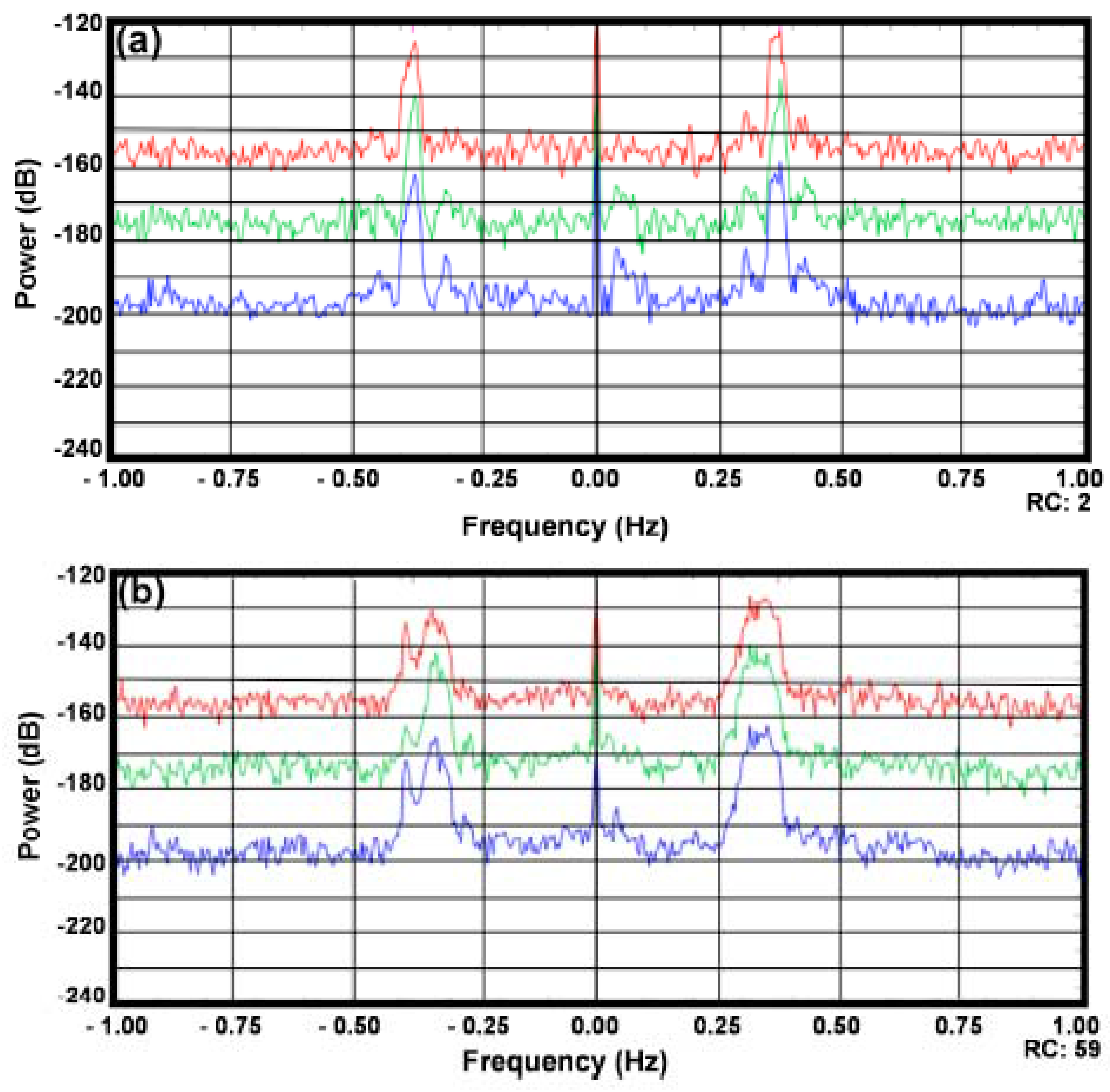
3. Derivation of Radial and Elliptical Velocities

In this section, we give the fundamental equations describing the radar spectra in terms of the current velocity field. Interpretation of these equations yields radial and elliptical components of the current velocity vectors.

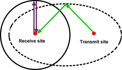
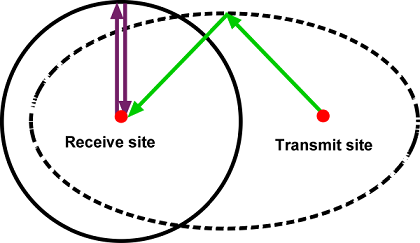
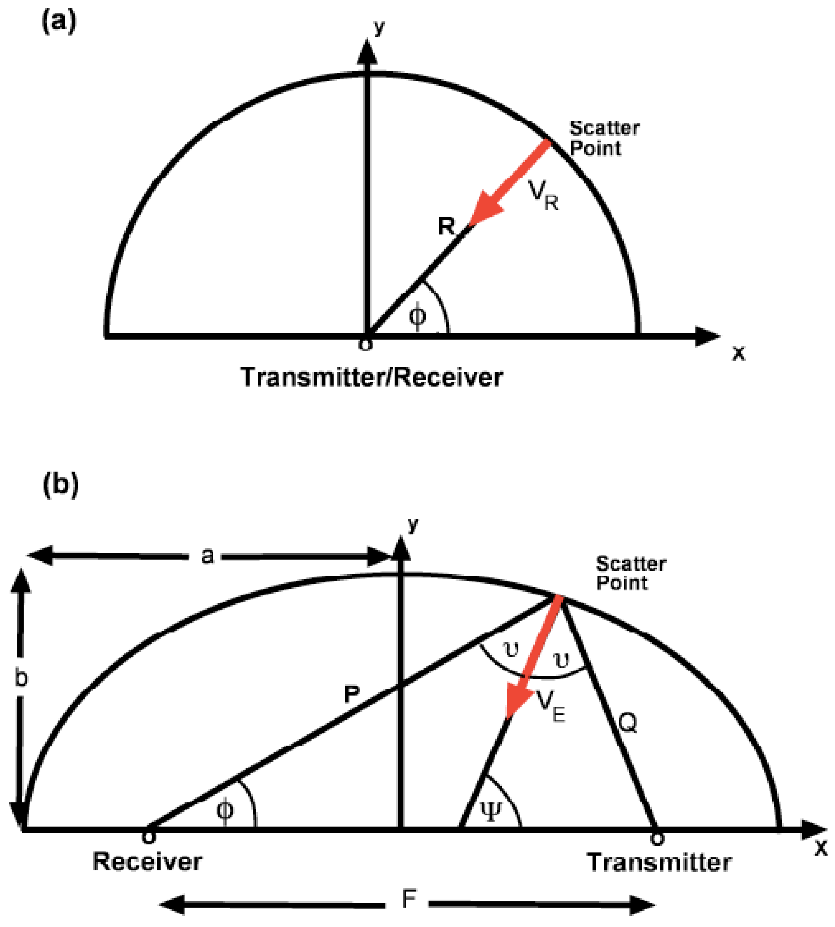
3.1. Radial Velocities

We now summarize the interpretation of backscatter echo to give estimates of radial velocities. When the receiver and transmitter are colocated, received echo signals with a given time delay arise from a range ring of constant radius from the transmitter/receiver, as illustrated schematically in Figure 3(a). The distance R to- and-from the radar to the range cell is given by:

$$R=2i\mathsf{\Delta }$$

(1)

where i is the range cell number and $\mathsf{\Delta }$ is the range cell width.

The Doppler spectrum of the received echo contains dominant peaks due to resonant Bragg scatter from ocean wave trains with wavelength one half the radar wavelength. In the absence of surface current motion, the peaks are delta functions at the Bragg frequencies ${\eta }_B$ defined in terms of the radar wavenumber $k_0$ by:

$${\eta }_B=\pm \sqrt{2g{k}_0}$$

(2)

where g is the gravitational constant. When currents are present, the echo is spread about these positions. The Doppler shift imposed by a current with a radial component $v_R(\varphi )$ at azimuth $\varphi$ is given by:

$$\delta \eta =2k_0{v}_R(\varphi )$$

(3)

The resulting power spectrum consists of peaks surrounding the ideal Bragg positions, see for example the backscatter spectra from the three SeaSonde receive antennas shown in Figure 4(a). For a description of the SeaSonde system configuration, see [7]. The width of the Bragg peaks increases proportionally to the radial current velocity. Voltages from the antennas are analyzed to give the radial velocity at each azimuth around the range circle.

Figure 3. Schematic diagrams of radar configuration (a) Backscatter from a circle of radius R around the transmitter/receiver location, showing azimuth angle ⎕⎕⎕of the received signal; (b) Bistatic scatter from an ellipse with receiver and transmitter at the focal points separated by distance F. Ellipse major and minor semi-axes a, b, are shown, as well as the azimuth angle φ⎕⎕⎕ of the received signal, the angles of incidence and reflection⎕⎕, the distances P, Q from the receiver, transmitter to a scatter point on the ellipse, and the slope⎕⎕ of the normal to the ellipse at the scatter point.

Figure 3. Schematic diagrams of radar configuration (a) Backscatter from a circle of radius R around the transmitter/receiver location, showing azimuth angle ⎕⎕⎕of the received signal; (b) Bistatic scatter from an ellipse with receiver and transmitter at the focal points separated by distance F. Ellipse major and minor semi-axes a, b, are shown, as well as the azimuth angle φ⎕⎕⎕ of the received signal, the angles of incidence and reflection⎕⎕, the distances P, Q from the receiver, transmitter to a scatter point on the ellipse, and the slope⎕⎕ of the normal to the ellipse at the scatter point.

An example of a measured radial velocity map is shown in Figure 5(a).

Figure 4. Radar echo spectra measured by an HF radar receiver located at Commonweal, California on April 02, 2008 23:10 (a) backscatter spectra, range cell 2; (b) bistatic echo spectra from the transmitter at Fort Funston, range cell 59.

Figure 4. Radar echo spectra measured by an HF radar receiver located at Commonweal, California on April 02, 2008 23:10 (a) backscatter spectra, range cell 2; (b) bistatic echo spectra from the transmitter at Fort Funston, range cell 59.

Figure 5. Radar current velocity maps produced by an HF radar located at Commonweal, California, on April 02, 2008, 23:10 from (a) backscatter; (b) bistatic echo from the transmitter at Fort Funston.

Figure 5. Radar current velocity maps produced by an HF radar located at Commonweal, California, on April 02, 2008, 23:10 from (a) backscatter; (b) bistatic echo from the transmitter at Fort Funston.

3.2. Elliptical Velocities

We now summarize the derivation of elliptical velocities from the radar echo power spectra; for more detail see [4]. Bistatic echoes result when the transmitter is separated from the receiver. The signal time delay is proportional to the distance traveled, which is the sum of the distances from the scattering patch to the transmitter and receiver. (In practice, an additional time delay is added as discussed in Section 2, to separate bistatic and backscatter echoes.) Therefore a fixed value for the time delay defines an ellipse with foci at the transmitter and receiver locations. We define the X-axis to pass through the transmitter and receiver locations, with the origin at the midpoint, see Figure 3(b). The angles of incidence and reflection $\upsilon$ defined with respect to the normal to the ellipse at any point are equal. With this configuration, the Bragg frequencies are defined by:

$${\eta }_B=\pm \sqrt{2g{k}_0\cos (\upsilon )}$$

(4)

As the magnitude of $\cos (\upsilon )$ is always less than unity, first-order peaks due to bistatic scatter trail off on the inner side of the ideal Bragg frequency , see for example the bistatic echo spectra shown in Figure 4(b). The additional Doppler shift from the Bragg frequency produced by a current with elliptical component $v_E(\phi )$ normal to the ellipse at azimuth $\phi$ is given by:

$$\delta \eta =2k_0{v}_E(\varphi )\cos (\upsilon )$$

(5)

For a given Doppler shift, we can determine the azimuth angles $\varphi$ of the received signal using the same direction-finding algorithms as for the backscatter case. If $\varphi$ is determined over a uniform grid spacing, it can be seen from Figure 2(b) that the angle will be bunched up behind the receiver and spaced far apart on the opposite side of the ellipse. This effect is most marked for the close-in ranges. SeaSonde software interpolates to produce even spacing of vectors as in Figure 4(b).

From the general properties of an ellipse it follows that the major and minor semiaxes of the ellipse, a and b, are given by:

$$a=\frac{P+Q}{2};b=\sqrt{a^2-F^2/4}$$

(6)

where F is the distance between the receiver and transmitter and the out-and-back distance , P+Q , follows from the measured time delay. P is given by:

$$P=\frac{(F-2a)(F+2a)}{2(F\cos (\varphi )-2a)}$$

(7)

It can be seen from Figure 3(b) that the coordinates x, y of the scattering point are given by:

$$x=P\cos (\varphi )-F/2:y=P\sin (\varphi )$$

(8)

The slope $\psi$ of the normal to the ellipse at point (x, y), which defines the orientation of the elliptic velocity component, is given by:

$$\psi ={\tan }^{-1}(a^{2}y/b^{2}x)$$

(9)

and the angle of incidence/reflection $\upsilon$ by:

$$\upsilon =\text{\hspace{0.17em}}\psi -\varphi$$

(10)

The elliptic velocity component $v_E$ can then be obtained from the Doppler shift using (5). An example of a measured elliptical velocity map is shown in Figure 5(b).

In practice, as described in Section 2, time-delay cells in the radar spectrum containing bistatic echo are purposely offset well beyond the range cells containing backscatter echo, relative to the cell number $i_{dc}$ which contains the direct signal from the transmitter. To derive the relationship between range and range-cell number corresponding to (1) for the backscatter case, take a point on the x axis of Figure 3(b) a distance $(i-i_{dc})\mathsf{\Delta }$ to the right of the transmitter, where $i$ is the range cell number, and $\mathsf{\Delta }$ is the range cell width. At this point it can be seen that:

$$P=F+(i-i_{dc})\mathsf{\Delta }Q=(i-i_{dc})\mathsf{\Delta }$$

(11)

The range R at this point is given by:

$$\begin{array}{l}R=P+Q=F\text{+2}(i-i_{dc})\mathsf{\Delta }\end{array}$$

(12)

Due to the properties of the ellipse, this relationship holds for all points around the elliptical time-delay cell.

There is a region around the baseline between transmitter and receiver that does not produce useful current measurements with bistatic geometries. For example in Figure 5b, the 57th time-delay cell contains the direct signal and vectors are shown only beyond the 59th time-delay cell. The primary reason is that the direct signal from the transmitter (i.e., the "zero" time-delay cell) is so strong that its temporal processing sidelobes falling in the first time-delay cells mask the Bragg regions needed for currents. Another reason for excluding the narrow inner ellipses is their wide spacing of vectors on the side of the ellipse opposite the receiver, which results in increased velocity uncertainties; see the discussion following (5).

3.3. Averaging and Uncertainties in Seasonde Radial and Elliptical Velocities

At a given location, there are typically several velocity values produced. These values are averaged to give the short-term output value for that location and the standard deviation is calculated. This uncertainty is due statistical noise in the data, variations of oceanographic conditions during the 10-minute spectral averaging period and horizontal shear within the radar cell and is termed the “spatial standard deviation”. Successive short-term radial/selliptical files are averaged or merged over a specified time period to produce then a longer-term map of averaged velocity components. The merged map is smoother and more filled-in at the expense of perhaps missing the shortest-term geophysical features. The merged output at a given location consists of the mean radial velocity, the spatial standard deviation, and the standard deviation of the mean, obtained from the variations within the merge-time of the short-term radial velocities. This uncertainty is termed the “temporal standard deviation”.

Even when the spatial standard deviation is high due large horizontal velocity shear in the radar cell, the average often does not vary significantly with time, leading to low values of the temporal standard deviation. Then measurements appear stable as a function of time and two radars operated side-by-side will produce similar results. It can be a different matter when a radar area measurement is compared with a buoy point measurement. Differences in the two velocity measurements don’t necessarily indicate inconsistency, if they are less than the error bars. Approximately equal values of the spatial and temporal uncertainties indicate that horizontal velocity shears within the radar cell are much less than stochastic variations. For a further discussion of this interpretation, see [7].

4. Drifter Comparisons and Radar Consistency Checks

In this section, we describe the results of an experiment to compare current velocities measured by HF radar and drifters from April 1 to 4, 2008. We will refer to radial, elliptical velocity components as ‘radials’, ‘ellipticals’ and total velocity vectors as ‘totals’.

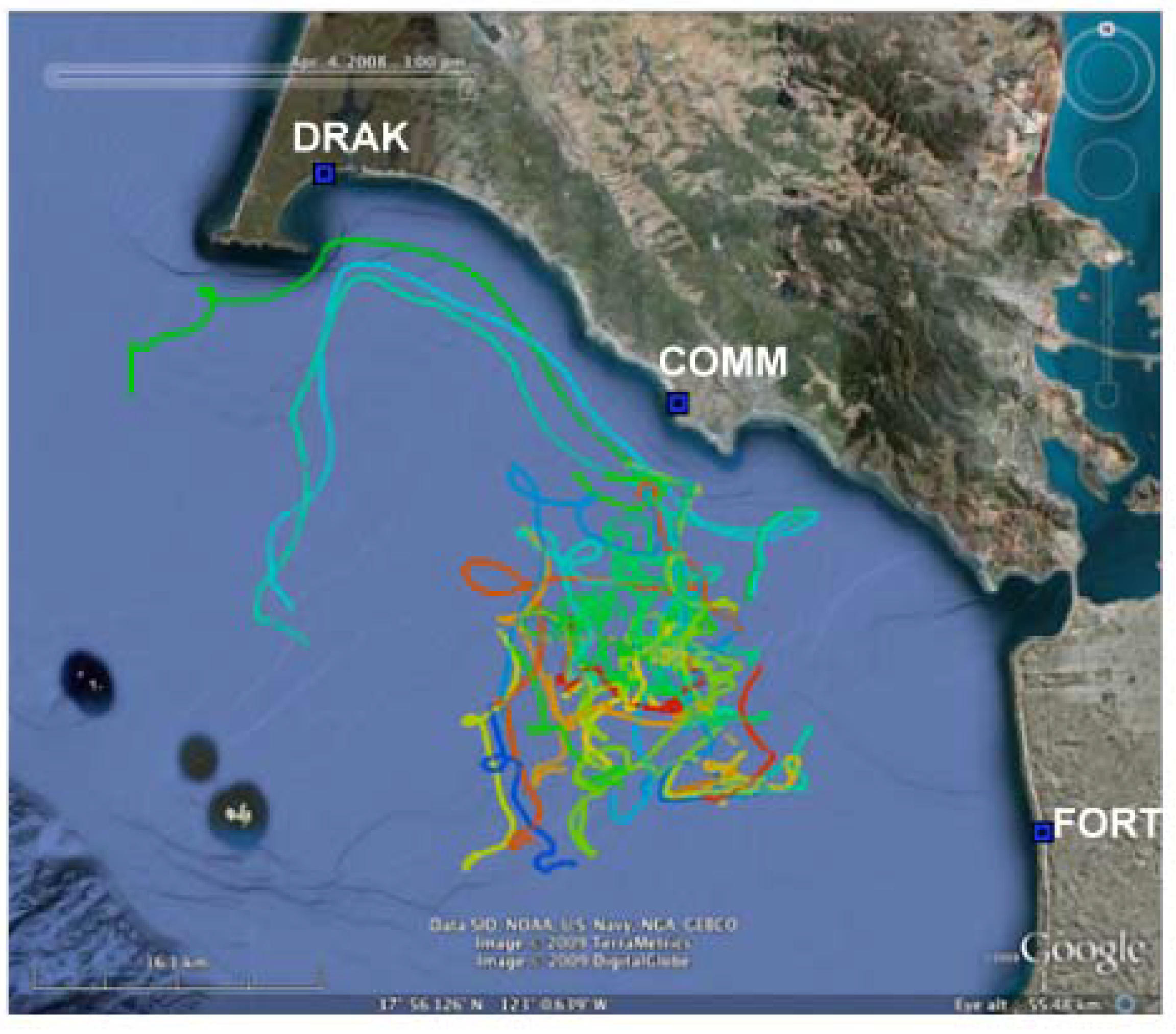
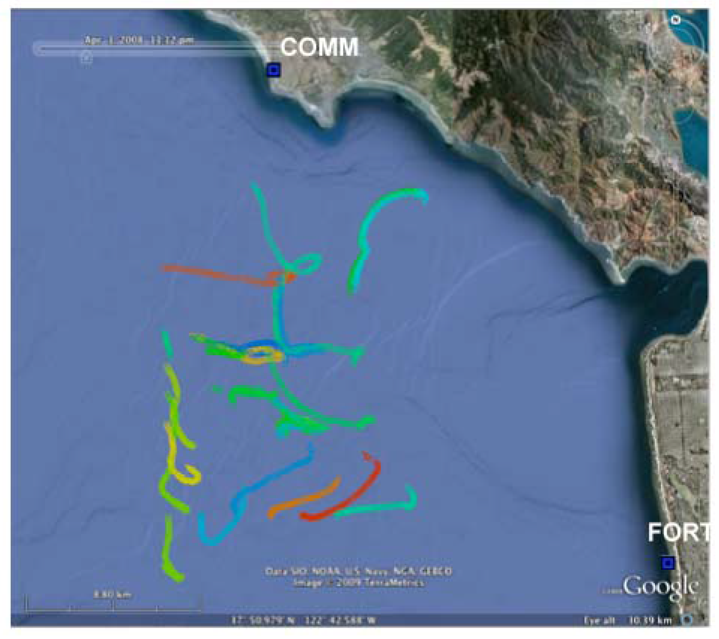
4.1. Drifter and Radar Measurements

During the experiment, 42 drifters were deployed outside of the mouth of the San Francisco Bay in the Gulf of the Farallones. Over the course of the experiment, there were light offshore and moderate onshore winds. Simultaneous radar measurements were made from six HF radar units located on the neighboring coastline. From these radars, we selected sites at Commonweal (COMM), Fort Funston (FORT) and Drake's Bay (DRAK) for further study, based on the low level of radar interference and optimal coverage of the drifter locations. The site locations are shown in Figure 5. The three radars transmitted with a center frequency of 12.19 MHz and recorded backscatter echo spectra. FORT also acted as a transmitter from which bistatic echoes were received at COMM. GPS-derived modulation offsets were set to 100 µs and 1,100 µs respectively for COMM and FORT, so that the FORT bistatic sea echo could be received at COMM. Sweep bandwidth was set to 51.3 kHz, giving a backscatter range cell width of approximately 3 km. Short-term radial velocities were obtained with a 10-minute time resolution.

To measure the receiver antenna patterns, a transponder was placed on a boat which traversed an arc at constant range transmitting signals that are picked up by the receiver. The received signals were then analyzed to produce the complex antenna voltage patterns to be used in the signal analysis. In this case, due to obstacles, the boat transporting the transponder could not go all the way up to the coast. The resulting antenna pattern measurements therefore had gaps at the southern edge and the full angular range of the sea-echo was not covered by the pattern measurement. This results in radial vectors crowding onto the radial spoke on the antenna pattern boundary and loss of accuracy in this region. Vectors falling on the edges of the antenna pattern were therefore eliminated; see [7] for further discussion of this effect.

The drifters (manufactured by Pacific Gyre Corporation, Oceanside, California) are comprised of a corner-radar-reflector-type drogue attached to a surface float that houses the electronics. The drogue is roughly 85 cm in diameter, and is centered at a depth of 1 m. The surface float is 20 cm in diameter giving a drag-area ratio of about 40. The drifters measure position, accurate to within a few meters, every 10 minutes with GPS. Figure 6 shows all the drifter tracks over the course of the experiment. Because of weak currents, the drifters are largely confined to a restricted area, as shown. Figure 7 shows drifter tracks over a 4-hour period when the currents were veering from an easterly to a westerly direction. The mean velocity and bearing were obtained from the position/time at each point on the drifter track, and that at preceding and succeeding points. Range and bearing of the drifter relative to COMM were calculated assuming that the signal path is a great circle.

Figure 6. Drifter tracks recorded from April 1 to 4, 2008 off the Northern California coast, with positions plotted as triangles, with a different color for each drifter.

Figure 6. Drifter tracks recorded from April 1 to 4, 2008 off the Northern California coast, with positions plotted as triangles, with a different color for each drifter.

Figure 7. Drifter tracks recorded from April 1, 2008 14:20 to 18:40 showing the currents veering from an easterly to a westerly direction.

Figure 7. Drifter tracks recorded from April 1, 2008 14:20 to 18:40 showing the currents veering from an easterly to a westerly direction.

Drifter velocities were then averaged in the same manner as radar velocities, so that a direct comparison could be made. Drifter velocities were averaged over the same 10-minute intervals as the radar velocities and were then averaged over each radar scatter patch. Thus radar and drifter velocities for comparison had the same times and locations, with a 10-minute time resolution and an area-resolution equal to the radar cell at that location. Resulting drifter velocities were then resolved into radial and elliptical components for comparison with corresponding radar results. Drifter and radial and elliptical files were then merged over hour intervals to produce the comparison data set.

To make radar/drifter comparisons at a given time, all data points were included for which a given radar cell contained both radar and drifter vectors. Radar cells at the angular boundaries of the antenna pattern measurement were excluded from the comparison as discussed previously in this section. No data points were excluded based on wind or wave conditions, or for any other reason.

4.2. Radar Consistency Checks

We used the following method to check the consistency within the radar data set. A rectangular grid was defined to cover the common coverage area. The radials from FORT and COMM were combined to form total velocity vectors using the vectors falling within an averaging circle of 5 km radius about each grid point. Figure 8 shows an example of a total vector map. Radial and elliptical radar cells were defined by 3 km range increments and 5° angular widths. Although these are radar-to-radar consistency checks, different measurements (e.g., different receiver, transmitter, etc.) went into these comparisons.

Figure 8. Radar total current velocity map produced from the radial velocities measured by the HF radars at COMM, FORT on April 02, 2008 23:10.

Figure 8. Radar total current velocity map produced from the radial velocities measured by the HF radars at COMM, FORT on April 02, 2008 23:10.

Two checks were performed:

(a)

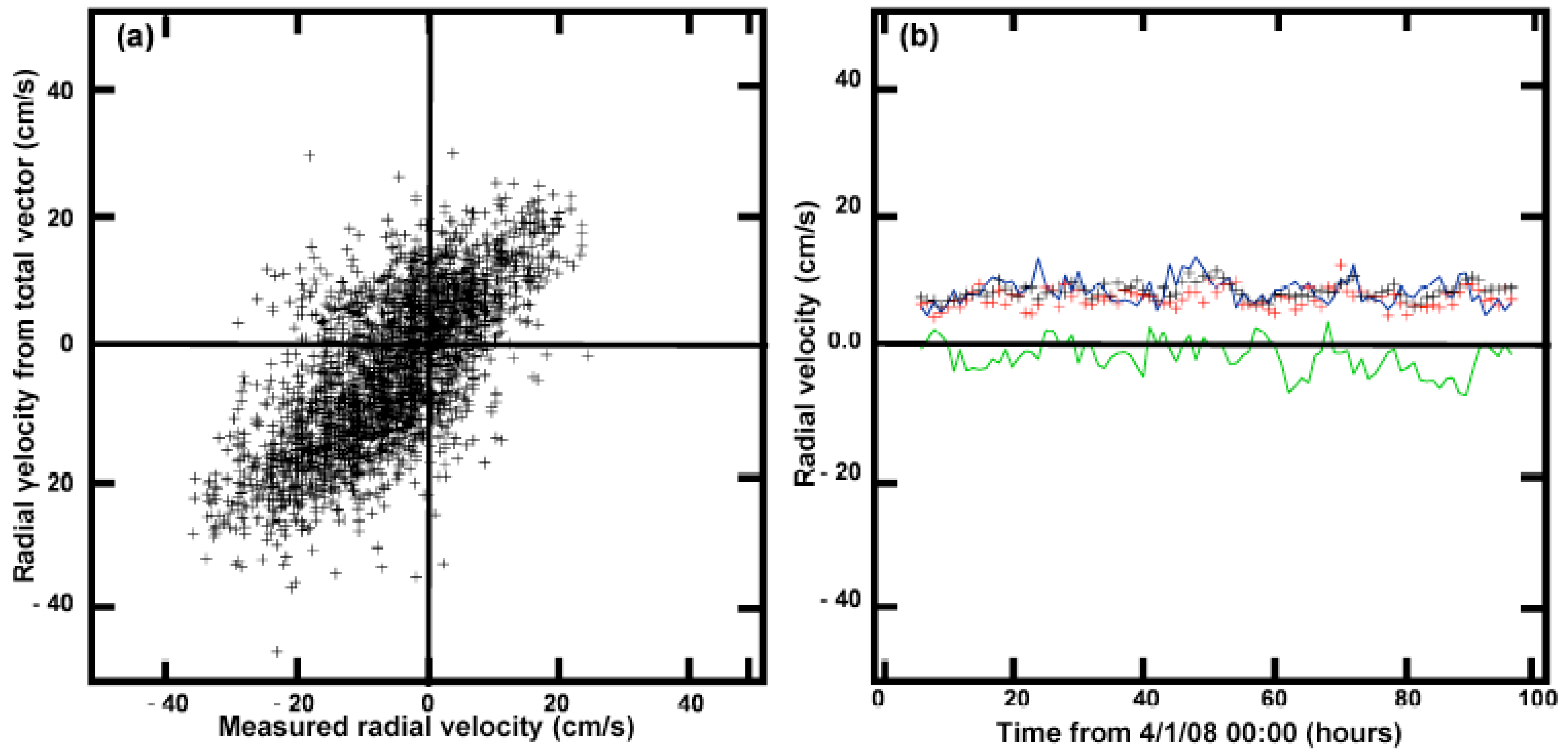
Consistency between measured radials and radials from a third site.

The total vector calculated from COMM/FORT radials was resolved in the direction pointing towards a third radar (DRAK) and the radials obtained from the totals were compared with those measured by DRAK. The comparison was restricted to cases for which there were at least 3 radial vectors from FORT, COMM and DRAK within the averaging circle. The unstable baseline region between the radar sites was excluded.

(b)

Consistency between measured radials and elliptical.

The total vector calculated from COMM/FORT radials was resolved in the direction perpendicular to the ellipse at each point and the elliptical calculated from the total velocity was compared with the measured ellipticals falling within the averaging circle. To be included in the comparison, there had to be at least three radial vectors from FORT and COMM within the averaging circle and at least three COMM elliptical vectors. This is an valuable consistency check between measured ellipticals from the recive site, and ellipticals obtained from measured radials from the receive/transmit sites. It uses data obtained from a single bistatic pair, with no need for ground observations. It can be carried out on a routine basis to provide validation for the measured ellipticals.

4.3. Comparison Methods and Results

As described above, there are four cases for comparison: (a) Radials, radar vs. drifter; (b) Ellipticals, radar vs. drifter; (c) Radar radials, measured vs. calculated from total vectors; (d) Radar ellipticals, measured vs. calculated from total vectors In each case, the following comparison methods were used:

(1)

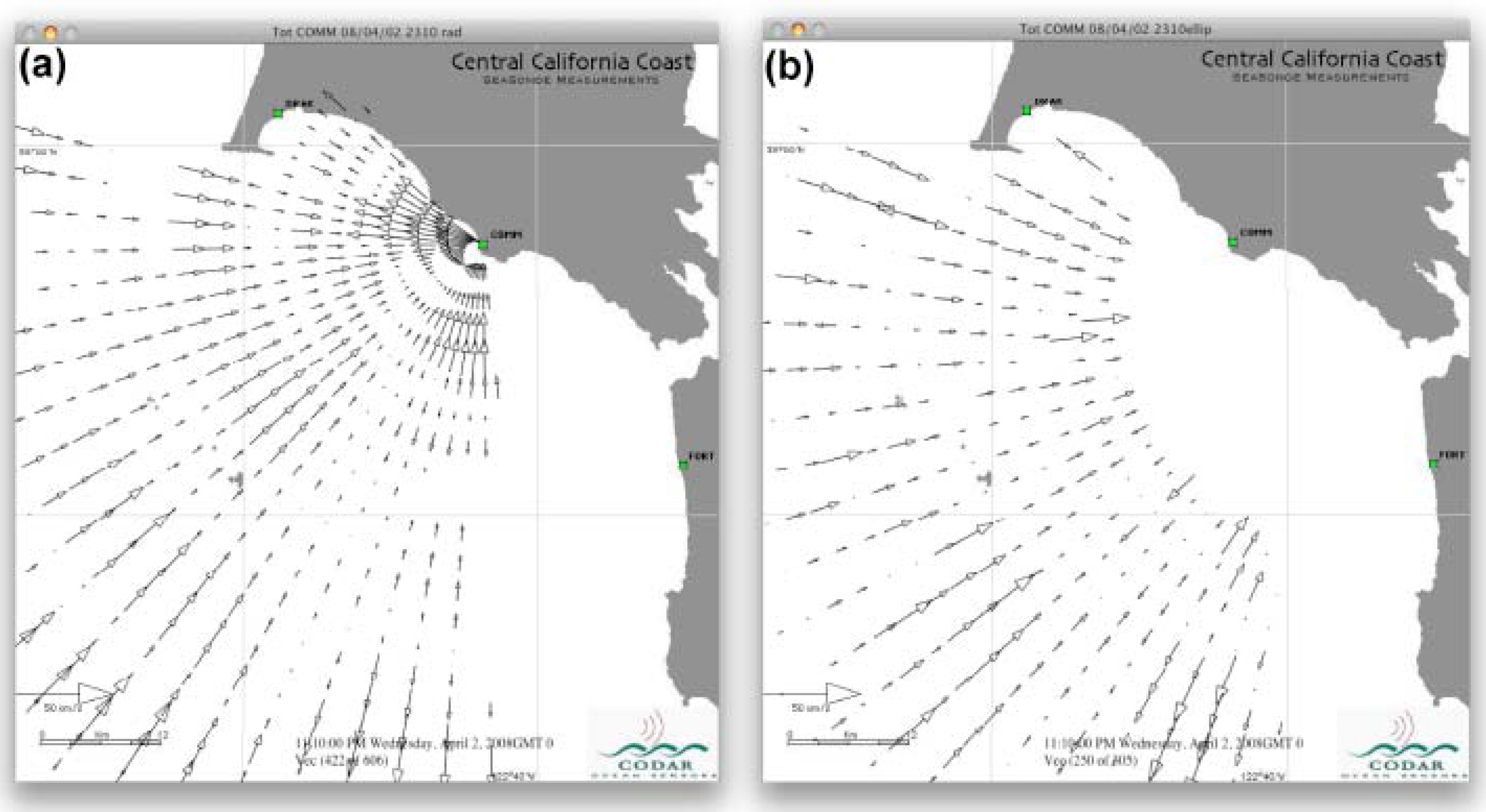
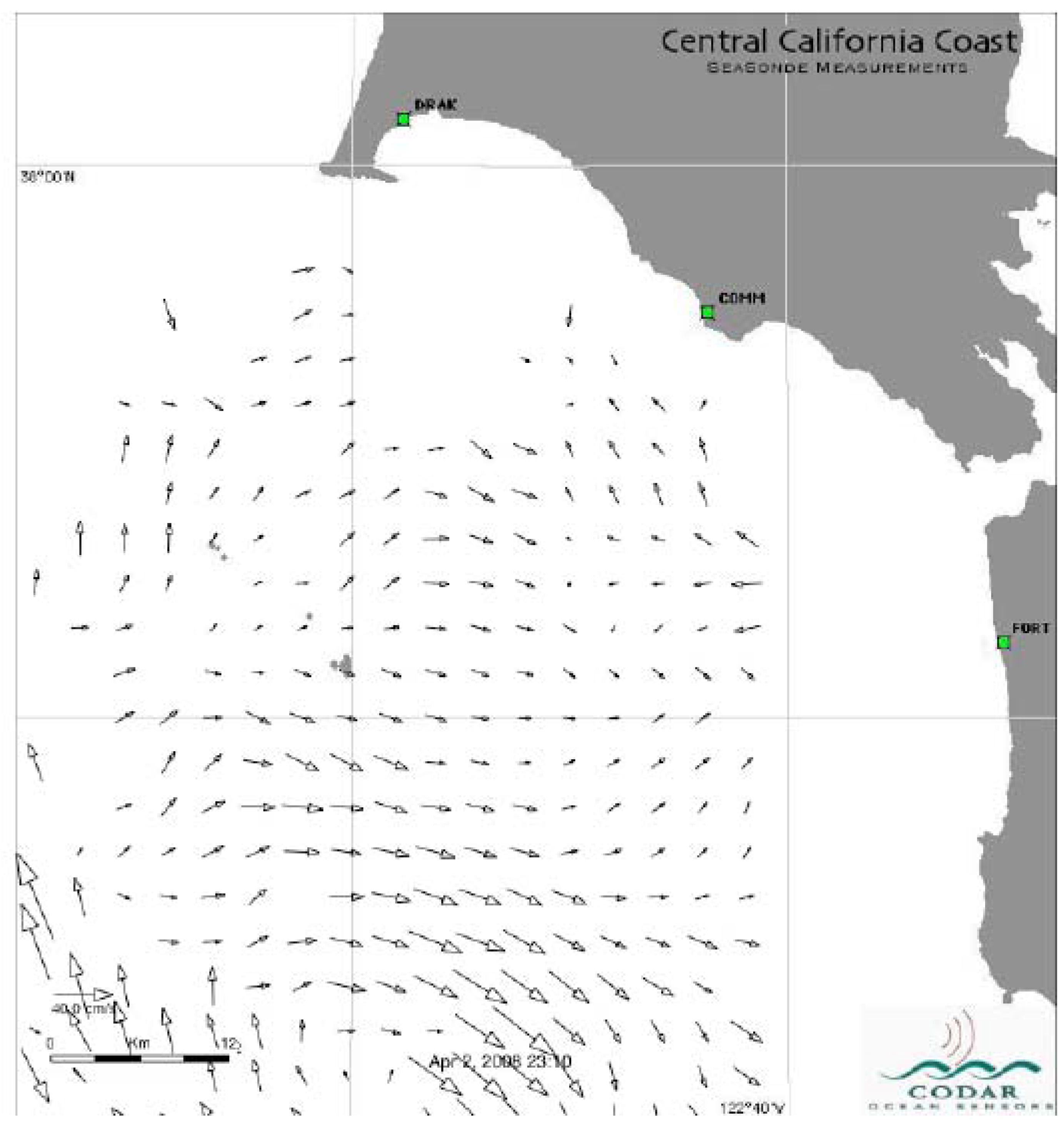
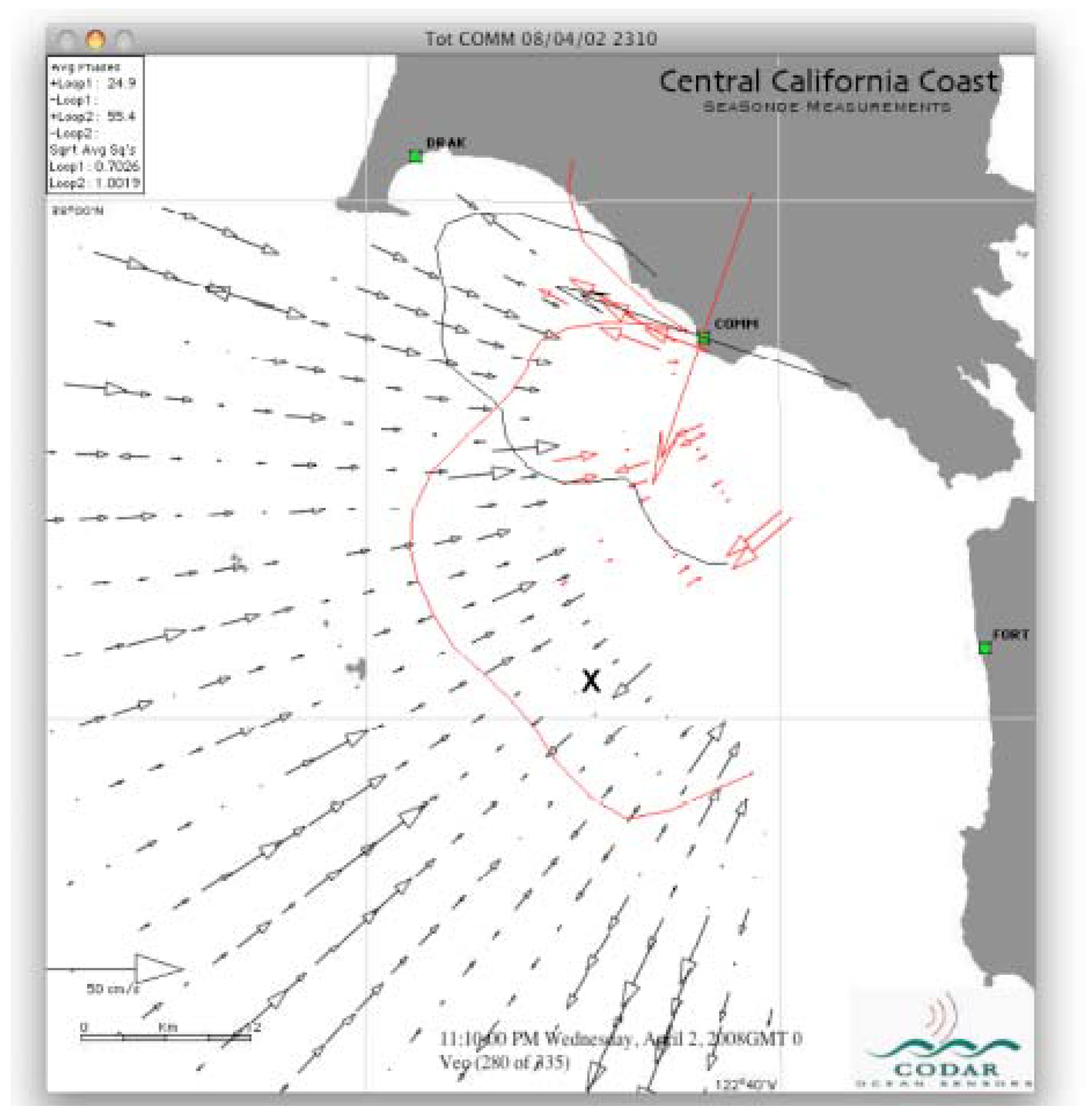
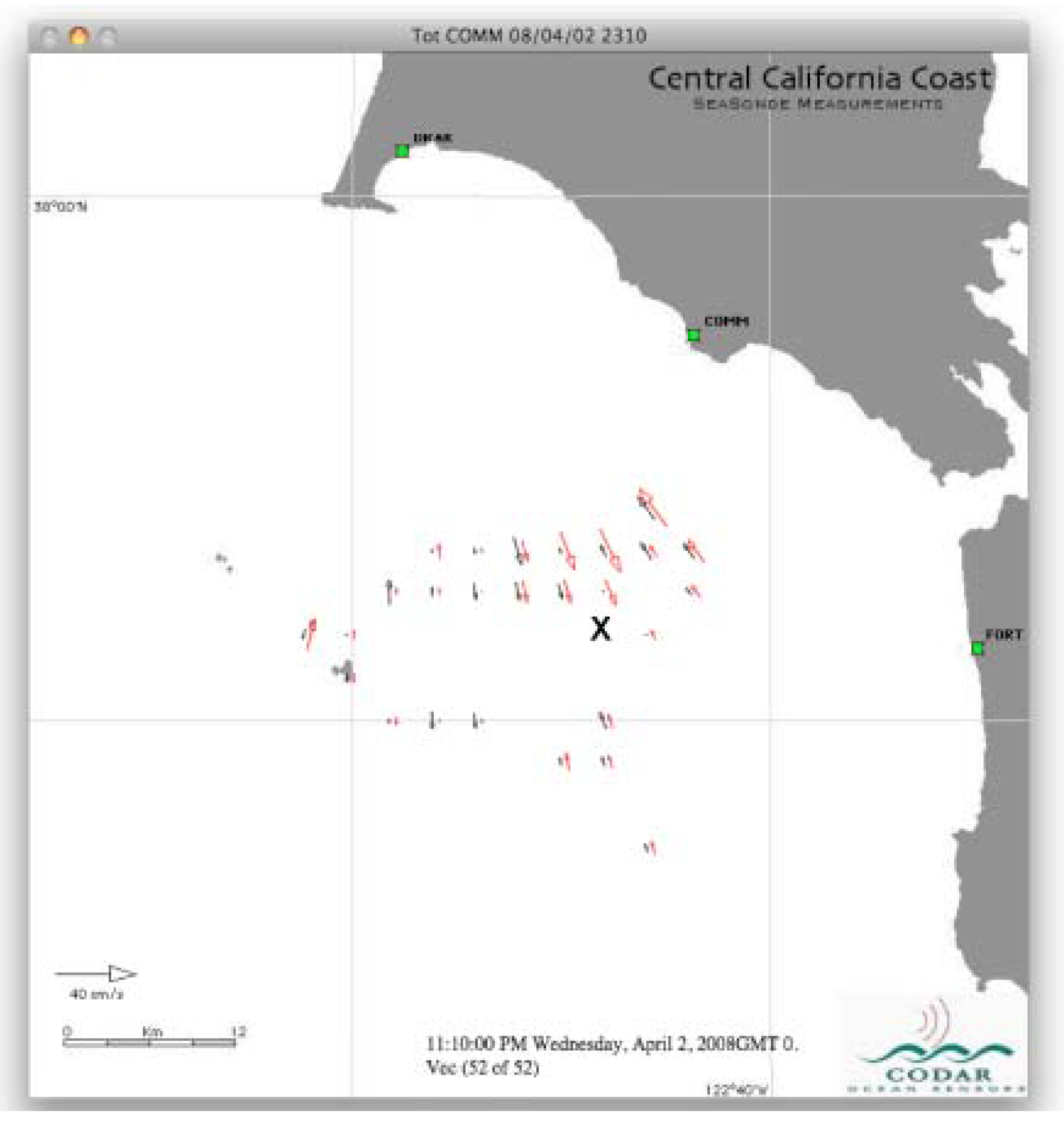
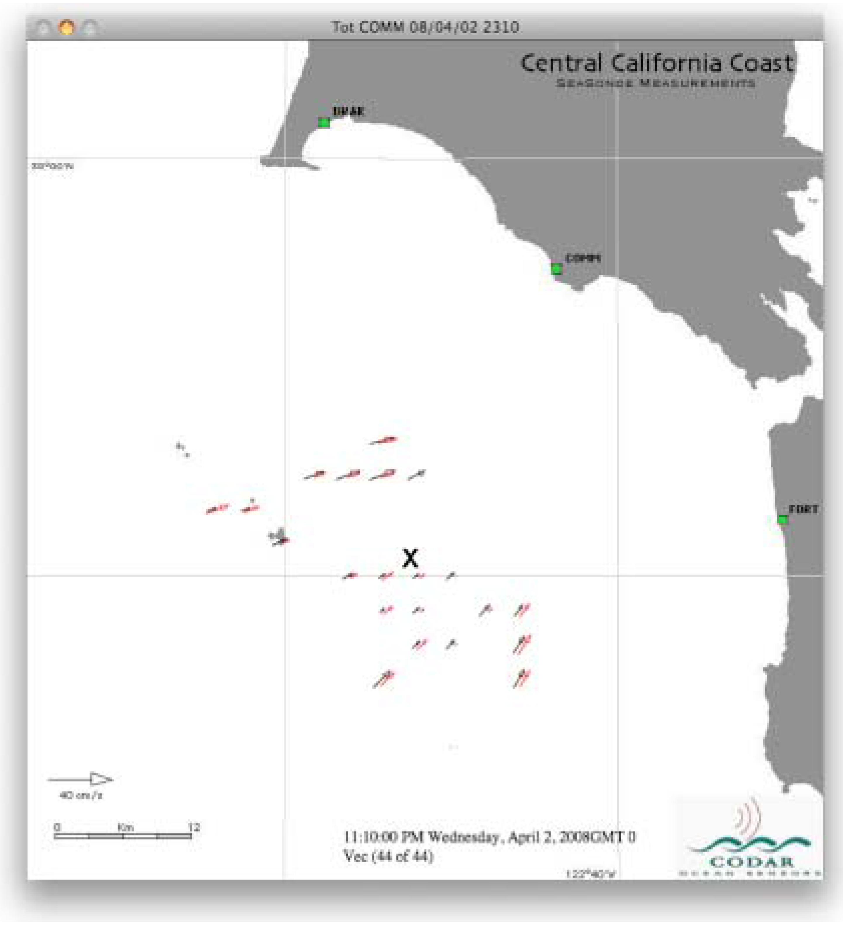
Movies were made of current velocity maps with the vectors being compared in different colors. We here show single frames; the movies can be downloaded from our web site at http://www.codar.com/.

(2)

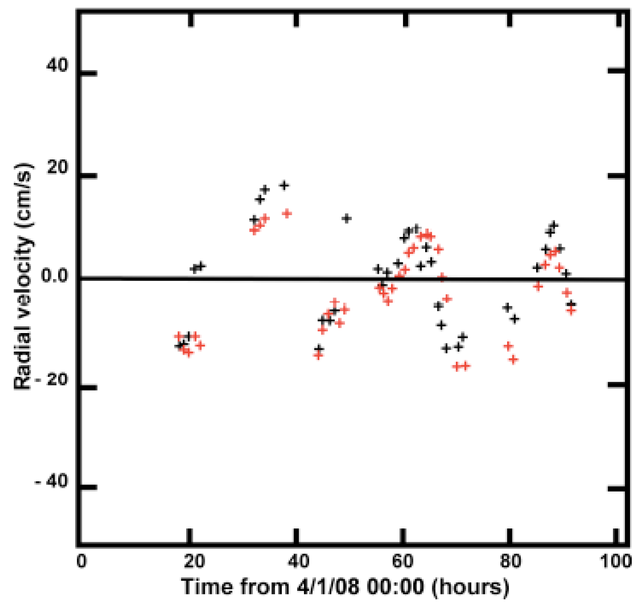
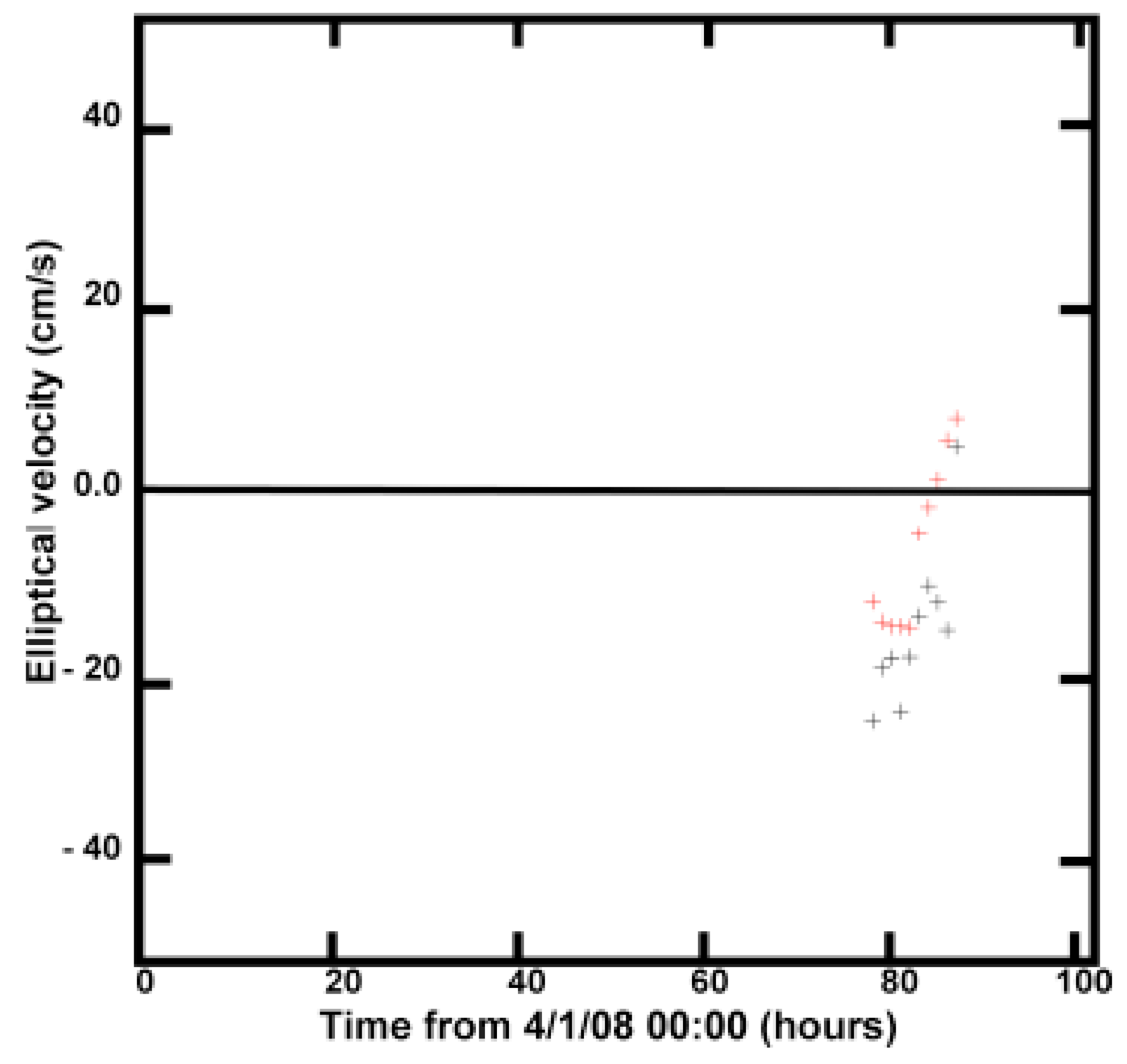
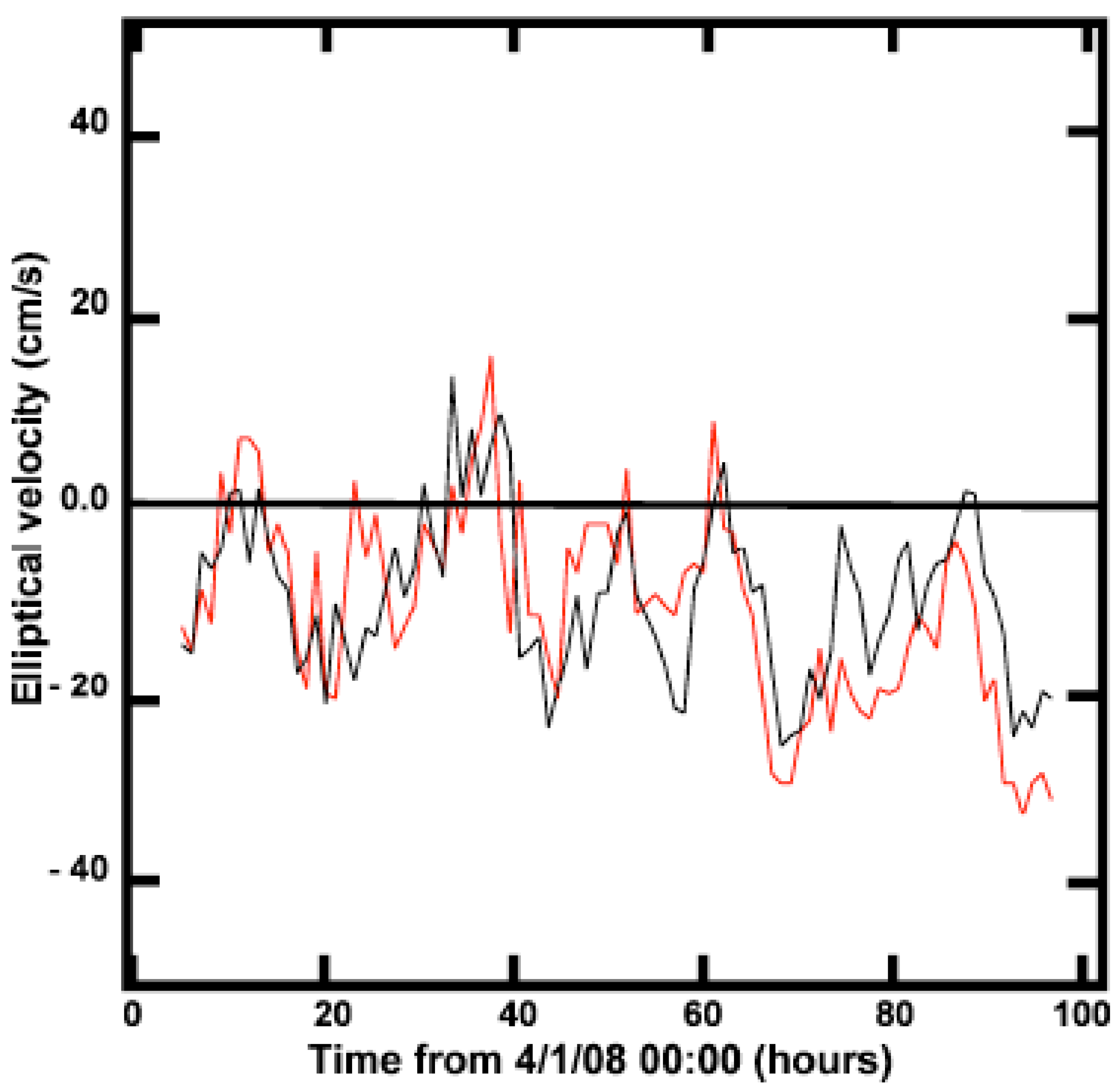
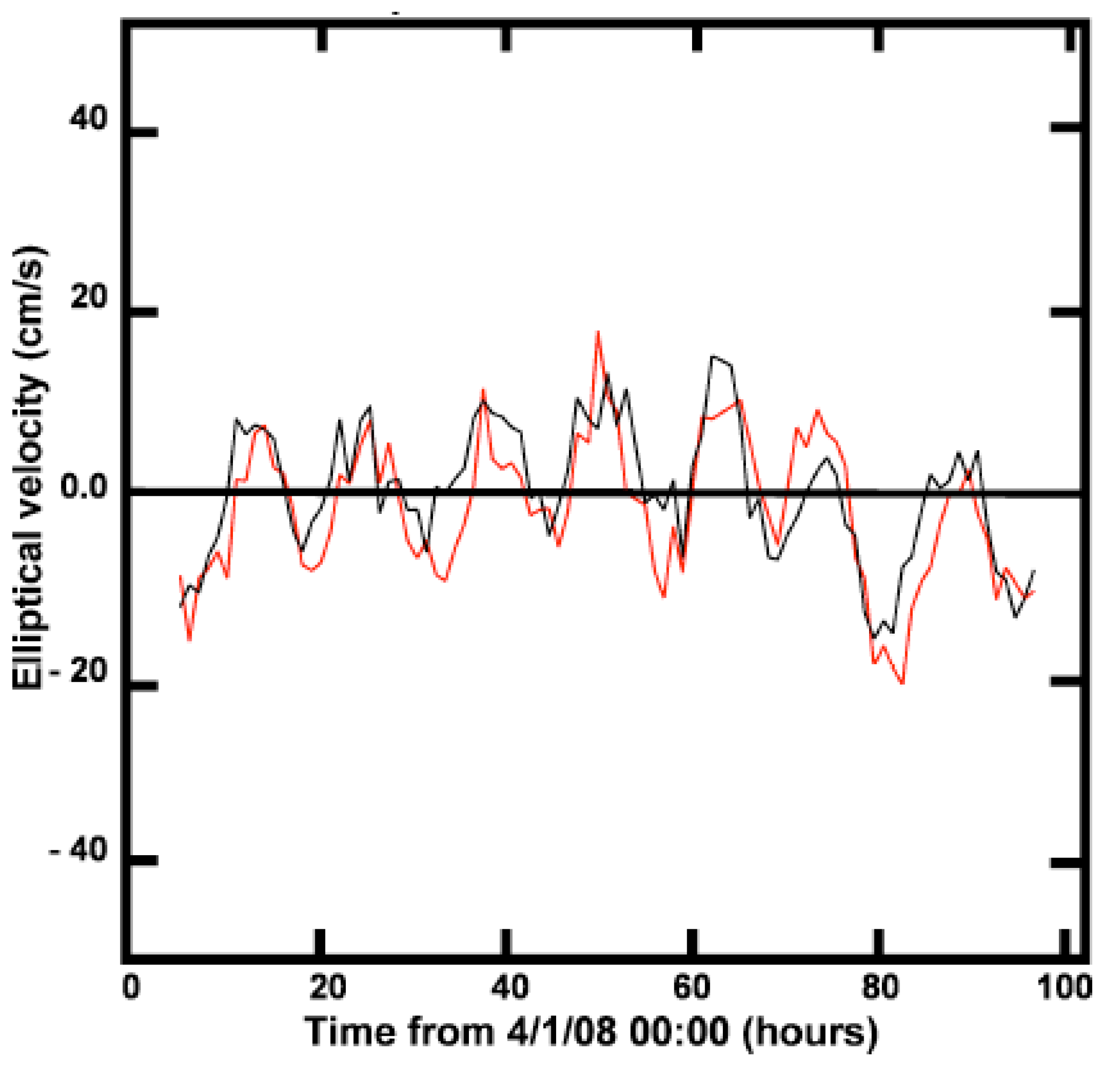
For illustration purposes only, compared vector components at a single location (marked X in the following maps) are plotted as a function of time. The location is chosen at random to include several drifter readings over time.

(3)

Comparison statistics calculated include standard deviations, biases, spatial and temporal uncertainties. These quantities are averaged over the map and plotted as a function of time. These values are further averaged over time and tabulated in Table 1 shown at the end of this section. Scatter plots are presented.

4.3.1. Radial Velocity, Radar vs. Drifter

Figure 9 shows an example of a comparison map, with drifter radials plotted in red. The location of the time series plotted in Figure 10 is marked with an X in Figure 9. Comparison statistics from the 1,287 available data points are plotted in Figure 11 and averaged values tabulated in the first column of Table 1. The mean standard deviation between drifter and radar radials was 8.5 cm/s, slightly larger than the radar spatial and temporal uncertainties (obtained directly from the radar files see [7]) of 6 cm/s, 6.4 cm/s respectively.

Figure 9. A comparison map of radial velocities measured by COMM (Black) and drifters (Red) on April 02, 2008 23:10. Time series of radial velocities at the point shown marked X are plotted in Figure 10.

Figure 9. A comparison map of radial velocities measured by COMM (Black) and drifters (Red) on April 02, 2008 23:10. Time series of radial velocities at the point shown marked X are plotted in Figure 10.

Figure 10. Time series of radial velocities measured at the point shown in Figure 9 by COMM (Black) and Drifter (Red).

Figure 10. Time series of radial velocities measured at the point shown in Figure 9 by COMM (Black) and Drifter (Red).

Figure 11. (a) Scatter plot of radial velocity data points: Drifter vs. radar; (b) Comparison statistics averaged over the map, plotted vs. time: Blue—standard deviation between radar and drifter radial velocities. Green—bias. Red—spatial standard deviation in COMM radials Black—temporal standard deviation in COMM radials

Figure 11. (a) Scatter plot of radial velocity data points: Drifter vs. radar; (b) Comparison statistics averaged over the map, plotted vs. time: Blue—standard deviation between radar and drifter radial velocities. Green—bias. Red—spatial standard deviation in COMM radials Black—temporal standard deviation in COMM radials

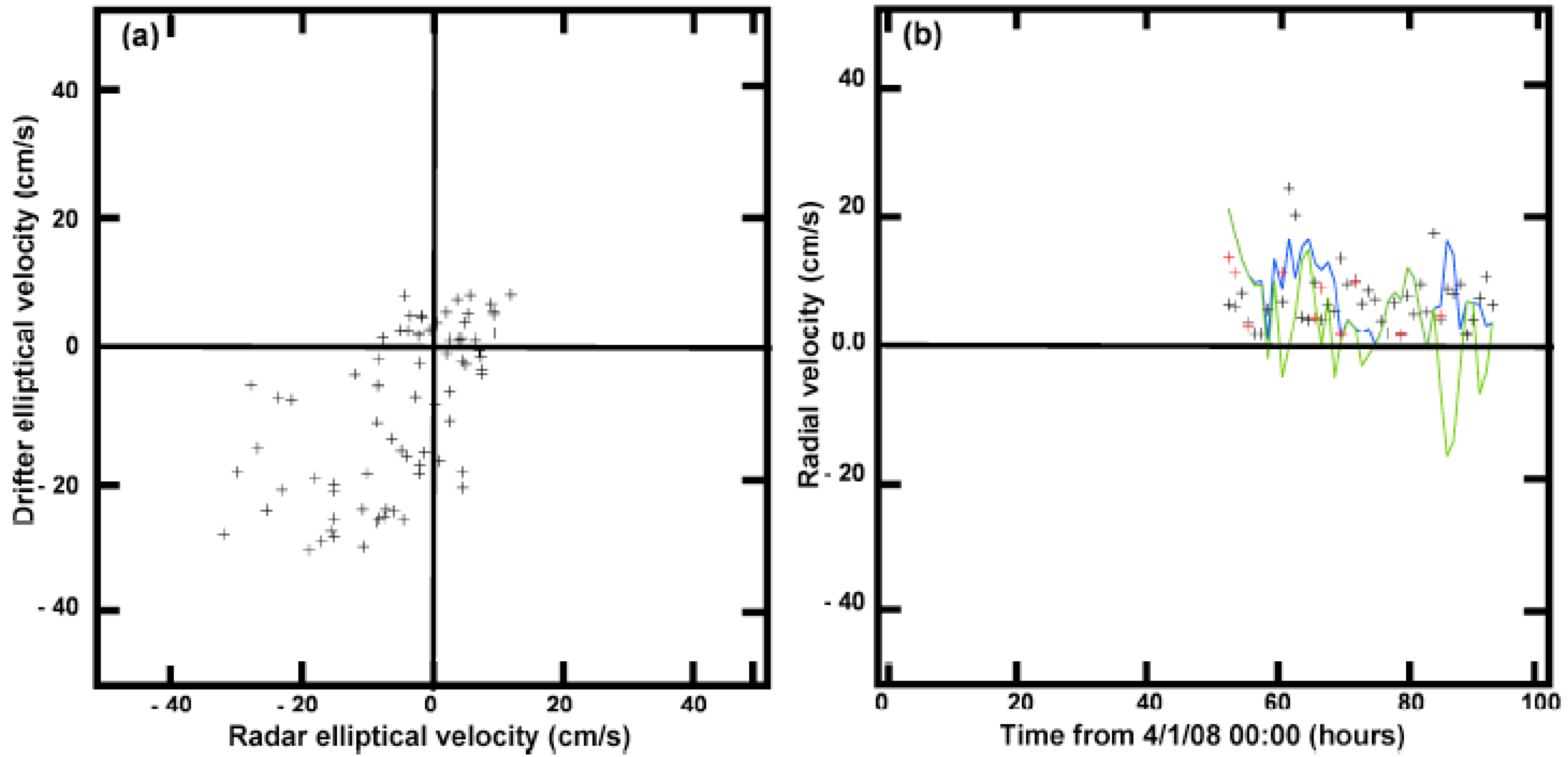
4.3.2. Elliptical Velocity, Radar vs. Drifter

Figure 12 shows an example of a comparison map, with drifter ellipticals plotted in red. Unfortunately there was little overlap of radar and drifter measurements over the course of the experiment. Furthermore, much of the overlap that occurred was close to the boundaries of COMM’s measured radar antenna patterns, which are drawn in Figure 12. Radar velocities are inaccurate in this region, as discussed in Section 4.1.

Figure 13 shows the compared ellipticals at the location indicated in Figure 12 plotted vs. time. Comparison statistics from the 75 available data points are plotted in Figure 14 and averaged values tabulated in the second column of Table 1. The mean standard deviation between drifter and radar radials was 10.9 cm/s, somewhat larger than the radar-estimated spatial and temporal uncertainties for these elliptical components (7.4 cm/s, 7.1 cm/s).

Figure 12. A comparison map of elliptical velocities, measured by COMM (Black) and drifters (Red) on April 02, 2008, 23:10. Time series of elliptical velocities at the point shown marked X are plotted in Figure 13. Normalized radar antenna patterns are shown: Loop 1 (black) ; Loop 2 (red).

Figure 12. A comparison map of elliptical velocities, measured by COMM (Black) and drifters (Red) on April 02, 2008, 23:10. Time series of elliptical velocities at the point shown marked X are plotted in Figure 13. Normalized radar antenna patterns are shown: Loop 1 (black) ; Loop 2 (red).

Figure 13. Time series of elliptical velocities measured at the point shown in Figure 12 by COMM (Black) and Drifter (Red).

Figure 13. Time series of elliptical velocities measured at the point shown in Figure 12 by COMM (Black) and Drifter (Red).

Figure 14. (a) Scatter plot of elliptical velocity data points: Drifter vs radar; (b) Comparison statistics averaged over the map, plotted vs. time: Blue—standard deviation between radar and drifter elliptical velocities. Green—bias. Red—spatial standard deviation in COMM ellipticals. Black—temporal standard deviation in COMM ellipticals.

Figure 14. (a) Scatter plot of elliptical velocity data points: Drifter vs radar; (b) Comparison statistics averaged over the map, plotted vs. time: Blue—standard deviation between radar and drifter elliptical velocities. Green—bias. Red—spatial standard deviation in COMM ellipticals. Black—temporal standard deviation in COMM ellipticals.

Figure 15. A comparison map of radial velocities. Black—calculated from total velocity vectors produced by COMM, FORT; Red—measured by DRAK. Time series of radial velocities at the point shown marked X are plotted in Figure 16.

Figure 15. A comparison map of radial velocities. Black—calculated from total velocity vectors produced by COMM, FORT; Red—measured by DRAK. Time series of radial velocities at the point shown marked X are plotted in Figure 16.

Figure 16. Time series of radial velocities measured at the point shown in Figure 15. Black—calculated from total velocity vectors produced by COMM, FORT. Red—measured by DRAK.

Figure 16. Time series of radial velocities measured at the point shown in Figure 15. Black—calculated from total velocity vectors produced by COMM, FORT. Red—measured by DRAK.

Figure 17. (a) Scatter plot of radial velocity data points: Radial velocity from COMM/FORT totals vs DRAK radial velocity; (b) Comparison statistics averaged over the map, plotted vs. time: Blue –standard deviation between DRAK radials and radials from COMM/FORT total velocities. Green—bias. Red—spatial standard deviation in DRAK radials Black—temporal standard deviation in DRAK radials.

Figure 17. (a) Scatter plot of radial velocity data points: Radial velocity from COMM/FORT totals vs DRAK radial velocity; (b) Comparison statistics averaged over the map, plotted vs. time: Blue –standard deviation between DRAK radials and radials from COMM/FORT total velocities. Green—bias. Red—spatial standard deviation in DRAK radials Black—temporal standard deviation in DRAK radials.

4.3.3. Radar Radial Velocity, Measured vs. Calculated from Total Vectors

Figure 15 shows an example of a comparison map, with DRAK radials plotted in red. Also indicated is the location of the time series plotted in Figure 16. Comparison statistics from the 2,810 points are plotted in Figure 17 and averaged values tabulated in the third column of Table 1. The mean standard deviation between radar measured and calculated radials was 8.5 cm/s, approximately equal to the radar-estimated spatial and temporal uncertainties (7.4 cm/s, 8.5 cm/s).

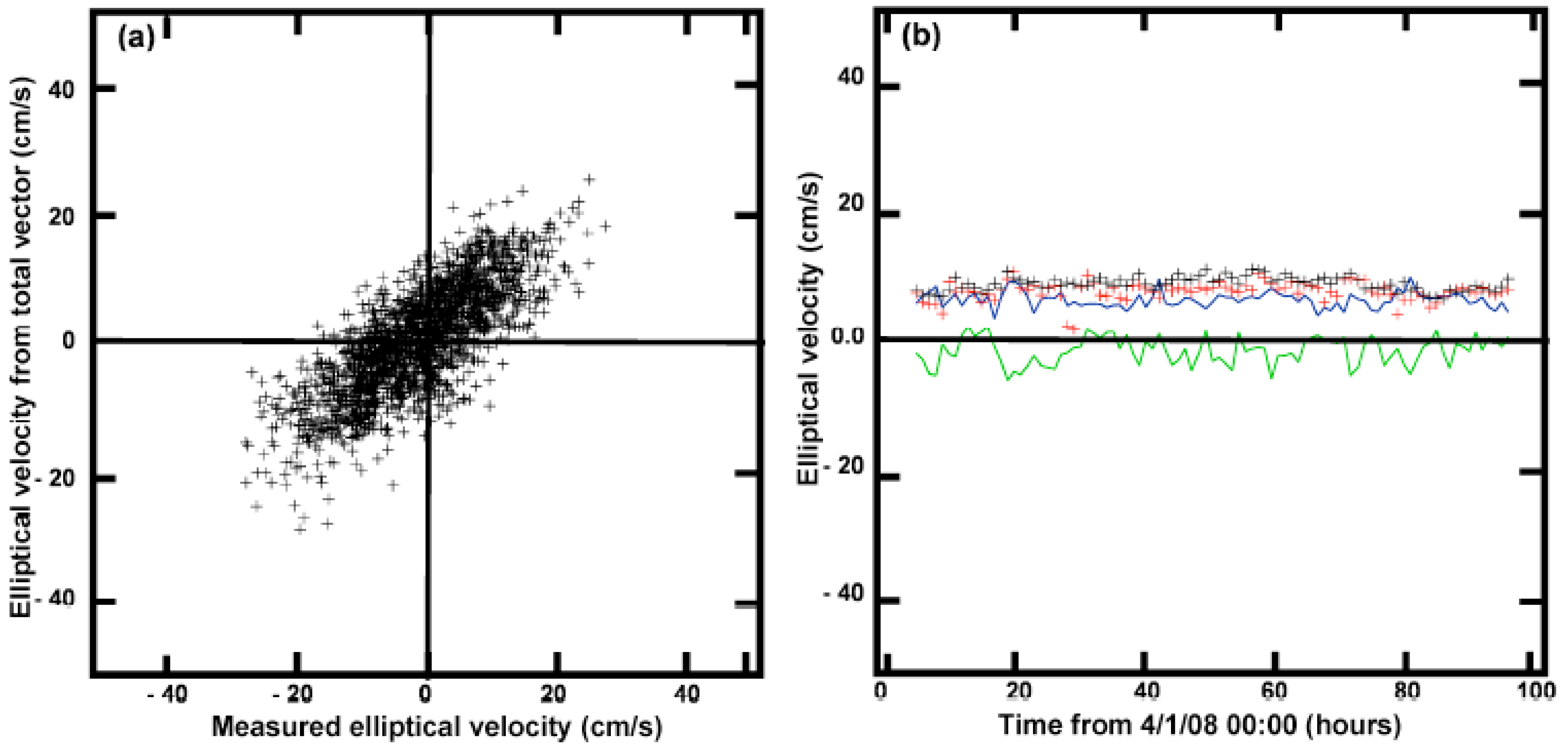
4.3.4. Radar elliptical Velocity, Measured vs. Calculated from Total Vectors

Figure 18 shows an example of a comparison map, with measured ellipticals plotted in red. Also indicated is the location of the time series plotted in Figure 19. Comparison statistics from the 1,957 points are plotted in Figure 20 and averaged values tabulated in the fourth column of Table 1. The mean standard deviation between radar measured and calculated radials was 6.1 cm/s, less than the radar-estimated spatial and temporal uncertainties (7.3 cm/s, 8.5 cm/s).

Figure 18. Elliptical velocity comparison map. Black—elliptical component of total velocity vectors from COMM, FORT. Red—measured by COMM. Time series of elliptical velocities at the point shown marked X are plotted in Figure 19.

Figure 18. Elliptical velocity comparison map. Black—elliptical component of total velocity vectors from COMM, FORT. Red—measured by COMM. Time series of elliptical velocities at the point shown marked X are plotted in Figure 19.

Figure 19. Time series of elliptical velocities measured at the point shown in Figure 18. Black—calculated from total velocity vectors produced by COMM, FORT. Red—measured by COMM.

Figure 19. Time series of elliptical velocities measured at the point shown in Figure 18. Black—calculated from total velocity vectors produced by COMM, FORT. Red—measured by COMM.

Figure 20. (a) Scatter plot of elliptical velocity data points: Elliptical velocity from COMM/FORT totals vs. COMM elliptical velocity; (b) Comparison statistics averaged over the map, plotted vs. time: Blue—standard deviation between COMM ellipticals and ellipticals from COMM/FORT total velocities. Green—bias. Red—spatial standard deviation in COMM elliptical.

Figure 20. (a) Scatter plot of elliptical velocity data points: Elliptical velocity from COMM/FORT totals vs. COMM elliptical velocity; (b) Comparison statistics averaged over the map, plotted vs. time: Blue—standard deviation between COMM ellipticals and ellipticals from COMM/FORT total velocities. Green—bias. Red—spatial standard deviation in COMM elliptical.

Table 1. Comparison statistics.

	Drifter vs. radar		Measured vs. calculated
	Radial	Elliptical	Radial	Elliptical
Velocity stats cm/s
Standard deviation	8.5	10.9	8.5	6.1
Bias	2	4.1	−1.8	−1.9
Radar uncerts cm/s
Spatial	6	7.4	7.4	7.3
Temporal	6.4	7.1	8.5	8.5

• Drifter vs. Radar:
• Column 1: Comparison between COMM and drifter radials
• Column 2: Comparison between COMM and drifter ellipticals
• Measured vs. calculated:
• Column 1: Comparison between DRAK radials and radials from COMM/FORT totals
• Column 2: Comparison between COMM ellipticals and ellipticals from COMM/FORT totals
• (Totals were calculated from COMM, FORT radials)

Table 1. Comparison statistics.

	Drifter vs. radar		Measured vs. calculated
	Radial	Elliptical	Radial	Elliptical
Velocity stats cm/s
Standard deviation	8.5	10.9	8.5	6.1
Bias	2	4.1	−1.8	−1.9
Radar uncerts cm/s
Spatial	6	7.4	7.4	7.3
Temporal	6.4	7.1	8.5	8.5

• Drifter vs. Radar:
• Column 1: Comparison between COMM and drifter radials
• Column 2: Comparison between COMM and drifter ellipticals
• Measured vs. calculated:
• Column 1: Comparison between DRAK radials and radials from COMM/FORT totals
• Column 2: Comparison between COMM ellipticals and ellipticals from COMM/FORT totals
• (Totals were calculated from COMM, FORT radials)

5. Conclusions

As in the previous section, we refer to radial and elliptical velocity components calculated from radar and drifter measurements as ‘radials’ and ‘ellipticals’. We have described the operation of an HF radar network to include essentially simultaneous reception of bistatic as well as backscatter radar echoes, for use in the estimation of current velocities.

Results are compared with drifter measurements. During the drifter deployment in April, 2008, drifters were mostly confined to a fairly small area. Unfortunately this area was largely disjoint from that covered by bistatic radar ellipticals. During the experiment, the spatial and temporal uncertainties were approximately equal, indicating small horizontal velocity shear within the radar scatter patch, as discussed in Section 3.3. Drifter velocity components were averaged using methods analogous to those used in radar analysis, and were resolved into components perpendicular to the circular and elliptical radar time-delay contours, allowing direct comparison with radar velocities. For radials, the mean standard deviation averaged over time and space was 8.5 cm/s, a factor of 1.3 larger than the mean temporal radar uncertainty. For ellipticals, the corresponding mean standard deviation was 10.9 cm/s, a factor of 1.5 larger than the mean temporal radar uncertainty. A reason for part of the larger standard deviation for ellipticals is the much sparser data set, over a shorter period of time and an area in which the radar vectors have reduced accuracy, as mentioned in the previous paragraph. Because of the consistency between the drifter/radar differences and the radar spatial/temporal uncertainties, it appears that the former are due mainly to current velocity variability within the radar cell and over the time of the measurement.

We then performed consistency checks on the radar radials, comparing radials obtained from the total velocities from a pair of radars with radials measured by a third radar site with overlapping coverage. The mean standard deviation was 8.5 cm/s, equal to the mean temporal radar uncertainty. Similarly, ellipticals obtained from the total velocities were compared with measured ellipticals from the bistatic echo. In this case, the mean standard deviation was 6.1 cm/s, which is actually less than the mean temporal radar uncertainty (8.5 cm/s).

In these comparisons, we find that there is good agreement between drifter and radar measurements. The differences are seen to be within the overall uncertainties derived from standard statistical analysis. We find that radar ellipticals are consistent with radar radials and that radar radials from three sites are consistent. The consistency checks between radar radials and ellipticals are performed routinely by the latest version of the Codar combining software. Thus although there were few drifter/radar ellipticals to compare, additional validation for radar ellipticals is provided by the agreement between the drifter/radar radials. HF radar backscatter observations of current velocity have been widely validated, see for example [8]. Therefore the routine establishment of consistency between radar radials and ellipticals in the future can be expected to provide support for the latter, as it does in this case.

References

- Teague, C.C.; Barrick, D.E.; Lilleboe, P.M. Geometries for streamflow measurement using a UHF RiverSonde. In Proceedings of the 2003 IEEE International Geoscience and Remote Sensing Symposium, Toulouse, France, 21–25 July 2003; pp. 4286–4288.
- Barrick, D.; Teague, C.; Lilleboe, P.; Cheng, R.; Gartner, J. Profiling river surface velocities and volume flow estimation with bistatic UHF RiverSonde radar. In Proceedings of the IEEE/OES Seventh Working Conference on Current Measurement Technology, San Diego, CA, USA, 13–15 March 2003; Rizoli, J.A., Ed.; pp. 55–59.
- Teague, C.C.; Barrick, D.E.; Lilleboe, P.; Cheng, R.T. Canal and river tests of a RiverSonde streamflow measurement system. In IEEE 2001 International Geoscience and Remote Sensing Symposium Proceedings, Sydney, Australia, July 9–13, 2001; pp. 1288–1290.
- Barrick, D.E.; Lilleboe, P.M.; Lipa, B.J.; Isaacson, J. Ocean surface current mapping with bistatic HF radar. U.S. Patent 6,774,837, 2004. [Google Scholar]
- Barrick, D.E.; Lipa, B.J.; Lilleboe, P.M.; Isaacson, J. Gated FMCW DF radar and signal processing for range/Doppler/angle determination. U.S. Patent 5,361,072, 1994. [Google Scholar]
- Barrick, D.E.; Lilleboe, P.M.; Teague, C.C. Multi-station HF FMCW radar frequency sharing with GPS time modulation multiplexing. U.S. Patent 6,856,276, 2001. [Google Scholar]
- Lipa, B.J.; Nyden, B.; Ullman, D.; Terrill, E. SeaSonde radial velocities: derivation and internal Consistency. IEEE J. Oceanic Eng. 2006, 31, 850–861. [Google Scholar] [CrossRef]
- Kohut, J.; Roarty, H.; Licthenwalner, S.; Glenn, S.; Barrick, D.; Lipa, B.; Allen, A. Surface current and wave validation of a nested regional HF radar Network in the Mid-Atlantic Bight, Current Measurement Technology. In Proceedings of the IEEE/OES 9th Working Conference, Charleston, NC, USA, 17–19 March 2008; pp. 203–207.
© 2009 by the authors; licensee MDPI, Basel, Switzerland. This article is an open access article distributed under the terms and conditions of the Creative Commons Attribution license (http://creativecommons.org/licenses/by/3.0/).
Share and Cite
Lipa, B.; Whelan, C.; Rector, B.; Nyden, B. HF Radar Bistatic Measurement of Surface Current Velocities: Drifter Comparisons and Radar Consistency Checks. Remote Sens. 2009, 1, 1190-1211. https://doi.org/10.3390/rs1041190
Lipa B, Whelan C, Rector B, Nyden B. HF Radar Bistatic Measurement of Surface Current Velocities: Drifter Comparisons and Radar Consistency Checks. Remote Sensing. 2009; 1(4):1190-1211. https://doi.org/10.3390/rs1041190
Chicago/Turabian StyleLipa, Belinda, Chad Whelan, Bill Rector, and Bruce Nyden. 2009. "HF Radar Bistatic Measurement of Surface Current Velocities: Drifter Comparisons and Radar Consistency Checks" Remote Sensing 1, no. 4: 1190-1211. https://doi.org/10.3390/rs1041190