Antarctic Ice Sheet and Radar Altimetry: A Review

Legos/OMP (CNRS-UPS), 14 av. Ed. Belin, Toulouse CEDEX 31400, France
*
Author to whom correspondence should be addressed.
Remote Sens. 2009, 1(4), 1212-1239; https://doi.org/10.3390/rs1041212
Submission received: 12 October 2009
/
Revised: 13 November 2009
/
Accepted: 28 November 2009
/
Published: 7 December 2009
(This article belongs to the Special Issue Microwave Remote Sensing)
Abstract
:Altimetry is probably one of the most powerful tools for ice sheet observation. Our vision of the Antarctic ice sheet has been deeply transformed since the launch of the ERS1 satellite in 1991. With the launch of ERS2 and Envisat, the series of altimetric observations now provides 19 years of continuous and homogeneous observations that allow monitoring of the shape and volume of ice sheets. The topography deduced from altimetry is one of the relevant parameters revealing the processes acting on ice sheet. Moreover, altimeter also provides other parameters such as backscatter and waveform shape that give information on the surface roughness or snow pack characteristics.
1. Introduction
Monitoring and understanding the Antarctic ice sheet are of great interest to address key scientific issues ranging from past climate conditions to potential future sea level rises [1]. Among all the remote sensing techniques applied to ice sheets, radar altimetry is particularly useful since it provides valuable information for meteorological studies, ice dynamics constraints and mass balance estimations. The aim of this paper is to give a review on the major glaciological progresses made thanks to this sensor.
1.1. The Antarctic Ice Sheet
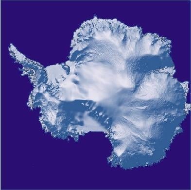
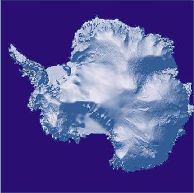
The Antarctic ice sheet has uneven bedrock, almost entirely covered by ice. Antarctica with a surface of 14 million km², and an average ice thickness of 2,200 m, represents 90% of the terrestrial ice and if melted could lead to an equivalent sea level rise of up to 60 m.
Figure 1.
Map of the Antarctic ice sheet with the main places cited in the text. Ice shelf names are in red.
Figure 1.
Map of the Antarctic ice sheet with the main places cited in the text. Ice shelf names are in red.
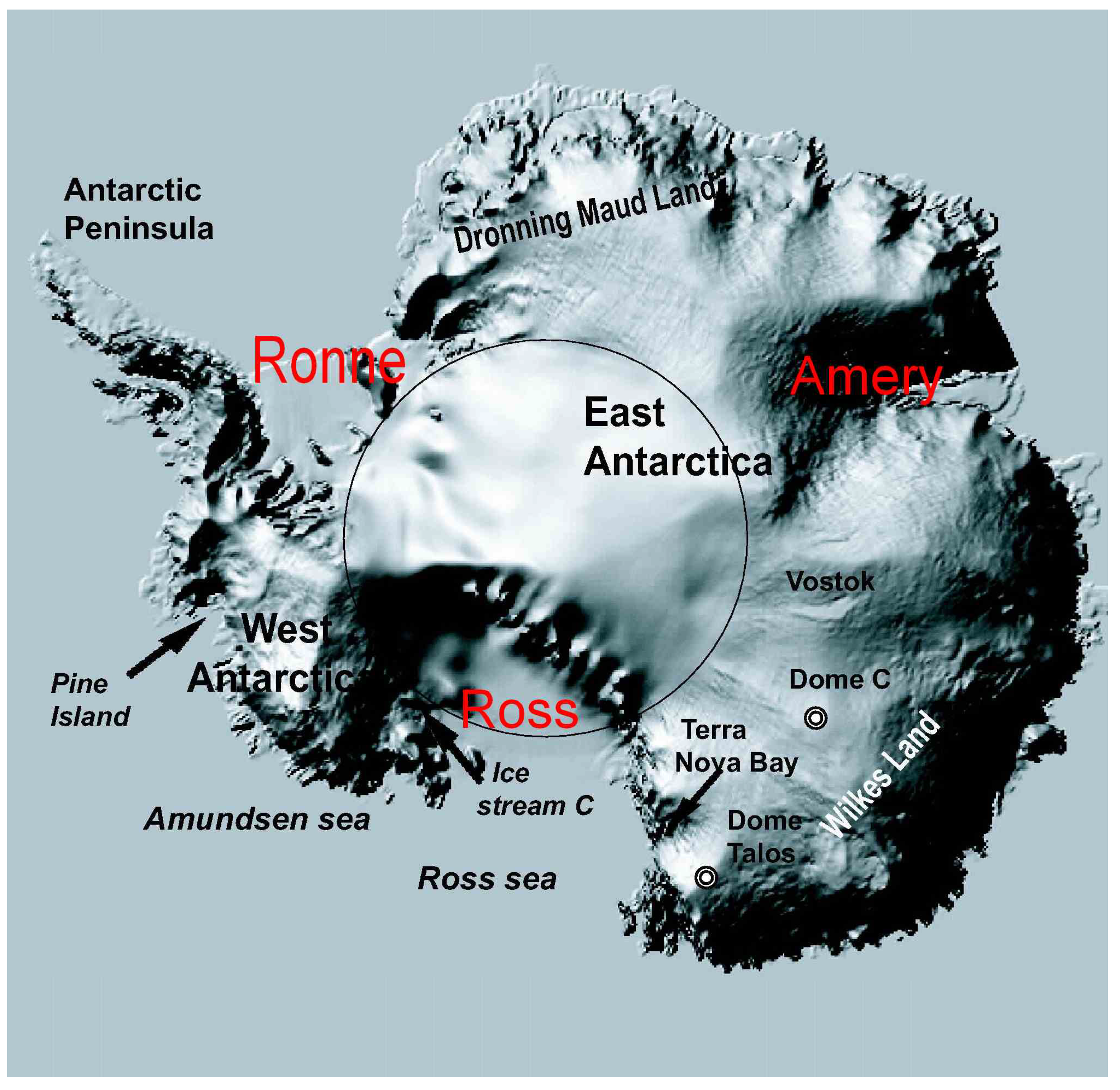
The Antarctic ice sheet is the coldest, highest, driest and windiest continent on Earth. The surface temperature decreases from the coast towards the interior from −15 °C to −60 °C. The cold and dense air of the interior rushes down the slope and can induce strong and persistent katabatic winds.
The altitude can reach up to 4,000 m in the Eastern part. The shape of the ice sheet is like a cap or a dome, with a very flat central part (the surface slope is less than 1 m/km over thousands of kilometres) so that the altimetric data are highly accurate. The ice sheet shape is controlled by the equilibrium between snowfall and ice flow [2]. The snow accumulation rate in Antarctica is less than a few centimetres per year in the interior and a few tens of centimetres near the coast [3]. That represents approximately 2,200 Gigatons each year or the equivalent of 6 mm of global sea level rise. A slight imbalance may then contribute to significant sea level changes.
The snow at the surface is buried by new snowfall and then sinks, turns into ice and flows down very slowly toward the coasts where it is calved. Ice velocity is extremely low in the centre of the ice sheets, less than 1 m/yr, and reaches 100 m/yr (or more) near the coast. It takes several hundreds of thousands years for the snow falling in the centre to reach the sea. This very long residence time is valuable for polar records. For instance, the EPICA depth ice core at Dome C allowed the recovery of 800,000 years of climatic history [4].
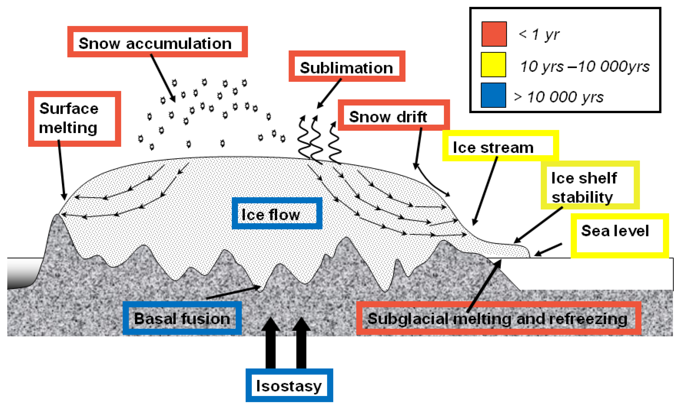
The quantity of snowfall and of ice calving or melting is known with large uncertainties of 20 or 30%, so that mass balance of polar ice caps is poorly known. Because of uncertainties, it is still very difficult to model these processes or even to determine their sign. First, the space and time distribution of accumulation rates is poorly known [5,6]. One of the difficulties lies in the distinction between snow precipitation and snow accumulation: the difference between both is due to erosion, drift, deposition by the wind or sublimation and all these processes are not very well known. Second, the physical processes which control the ice deformation or the ice sliding, the effect of the boundary conditions, or the effect of the longitudinal stress are still unknown. Moreover, precipitation rates or evaporation change in response to the climatic variations while the dynamic answer of the ice sheet to climatic changes would occur over a few tens of thousands years. As it is outlined on Figure 2, the range of the time scales of the different processes acting on an ice sheet is very large [7]. The variation of the ice sheet volume is due to climate changes over the last 100,000 years. As we will see in more details later, the Western part gets most of its bedrock under the sea surface and ice flows through a complex ice stream network, so that questions of instability or collapses arise.
Figure 2.
Ice sheet mechanisms and time-scale outline adapted from [7]. Surface melting, snow precipitation, sublimation, wind-driven sublimation and basal melting or refreezing are assumed to instantaneously react to climate change. Ice streams, outlet glaciers are assumed to react quickly (between 1 yr to 10 yr) or slowly as ice-shelf dynamics to climate change (meaning between 100 and 1,000 yr). On the contrary, ice flow, basal temperature and fusion isostasy take a very long time to react (time lag is between 10,000 and 100,000 years).

To understand, model or predict the ice sheet evolution, we then need to know climatic and dynamic processes which control them. We also need repetitive observations at a global scale to feed the models.
1.2. Observations of the Antarctic Ice Sheet
Its size is such that a few observations along traverses cannot render the main characteristics. For instance, in Antarctica, scientific stations are mostly near the coast, and only a few traverses during austral summer expeditions provide sparse data on the interior. In this context, remote sensing has offered during the last few decades a new vision of the polar cryosphere. The first sensor able to observe the cryosphere properties was the radiometer, acting in the microwave domain and devoted to atmospheric science. It was launched in the middle of 1970s allowing then a 30-yr record of variability of Antarctic sea ice [8]. Surface temperatures were not easy to derive from these first measurements but they allowed the precise delimitation of ice covered sea and the characterization of ice sheet’s surface. Today, several sensors give a precise idea of albedo, temperature, wind, surface velocity for continental ice (see Bindschadler [9] or Masson and Lubin [10] for a review of remote sensing of the Antarctic ice sheet). However, a lot of parameters, such as accumulation rate, ice thickness… are still poorly retrieved.
In this context, radar or laser altimetry plays a crucial role. Indeed, among parameters, surface topography is probably the most relevant [11]. From a dynamic point of view, surface topography can be used to constrain ice flow models, to test or initialize them. Ice physical processes often have a specific signature on the ice surface. Note that for ice dynamics study, the bed topography is also crucial. From a balance point of view, monitoring the surface elevation changes inform us about volume variations, we have now 19 years of continuous measurements at our dispoal. Here we will focus on radar altimetry because time series are longer and because it also provides subsurface information. Indeed, due to the penetration of the microwave within the snowpack, radar altimetry has the peculiarity of giving information not only on surface but also subsurface state that can be related to meteorological and climatic parameters [12].
The next section (2) is devoted to radar altimetry and will be followed by a section dealing with the physics of the measurements and on the snowpack properties retrieval. The last two sections (4 and 5) are devoted to the main purpose of altimetry above ice sheet, e.g., dynamics study derived from topography and monitoring of volume changes.
2. Radar Altimetry
Altimeter was initially designed to survey oceanic surface and error budget above the ice sheet should be carefully checked. The general concept can be found in Fu [13,14]. The principle consists in a radar wave emitted in the nadir direction and received by the sensor after reflection on the surface. The surface height is derived from the duration of the travel and the precise knowledge of the satellite orbit.
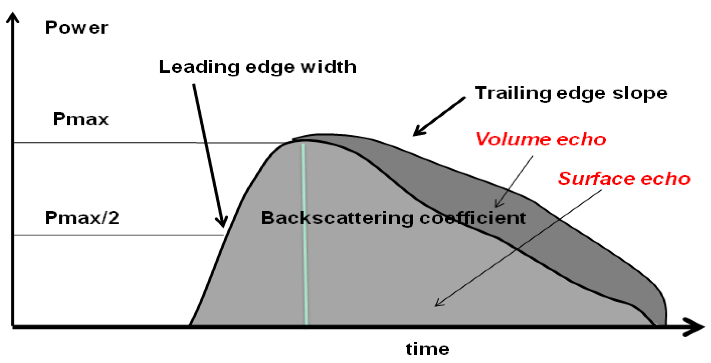
The sensor records the energy backscattered from the surface and the subsurface versus the arrival time, so that the total backscattered energy is available as the histogram of the energy with respect to time, the so-called waveform, in which lots of information lie (see Figure 3).
After correction due to the propagation delays through the atmosphere and ionosphere, instrument bias, terrestrial and oceanic tides, an altimeter such as the one onboard the Topex-Poseidon mission reaches a very good precision over oceans: it enables the estimation of global mean sea surface topography at the centimetric level at the 10-km scale [15] and sea level change with a precision better than 0.4 m m/yr [16]. However, when applied to continental surfaces, such as ice sheets, the error budget is greater and some specific corrections should be applied. Without going into details, let us summarize just the main specificities of the radar altimeter processing.
The first difference is due to the fact that classical atmospheric propagation corrections cannot be applied over ice surface. The radiometric or the dual-frequency observations used over oceanic surface to correct respectively for the wet troposphere and for the ionosphere delays are affected by snow surface signature and cannot be used to deduce respectively atmospheric wetness and electronic content as it is the case over oceanic targets.
A second difference is due to the kilometric-scale topographic features and surface slope that induce several problems. The altimeter measures the range between the antenna and the nearest point of the surface. This point is at the nadir only when the topography is very flat, otherwise it is shifted in the upslope direction of the surface. This error, pointed out by Brooks et al. [17] or Brenner et al. [18] depends on the square of the surface slope so that, near the coast of Antarctica, the restitution of a precise topography in such places is complicated. The correction can be done either directly on the height at the nadir or by relocating the impact point in the upslope direction [18,19,20,21]. The limitation is due to the lack of knowledge of the 2-D surface slope that can be derived from an external base [22] or by iteration from an a priori DEM obtaining by fitting a bi-quadratic form over the local area [21]. Nevertheless, data processing can be developed to correct for (or minimize) these errors so that altimeter measurements reach a very good accuracy. However, due to the inaccurate repetitivity of the orbit, the cross-track slope misknowledge is still one of the greatest limitations for the time series analysis (see Section 5). The kilometric scale feature also affects the tracking system which pre-positions the receiving window based on previous measurements and that cannot follow the irregular surface topography. The on-board estimate is thus inaccurate and a re-estimation, named retracking is needed. The process has to be applied with the help of the whole waveform [23]. Most of the existing retracking methods deduce the surface height elevation by seeking the point of the leading edge corresponding to the average surface [23,24,25]. Finally, due to the kilometric scale footprint, the small-scale topographic features also affect the waveform shape that in turns via the retracking affects the height restitution so that the final precision is limited [26]. The ICE-2 retracking algorithm, now implemented on the ground segment of the ENVISAT RA-2 altimeter is based on the principle of fitting the waveform shape using a classical model. It consists in detecting the waveform edge, fitting an error function to the leading edge and an exponential decrease to the trailing edge [27], so that three other altimetric parameters are provided in addition to the surface height (see Figure 3).
The third difference with classical ocean processing lies in the penetration of the radar wave within the snow pack. In Ku-band (13.6 GHz or wavelength of 2.3 cm), the classical altimetric band penetrates within the dry and cold snowpack so that the reflection comes both from the surface (called the surface echo) and subsurface layering (volume echo). This was first pointed out by Ridley and Partington [28] who modeled the waveform shape and detected a distortion due to the volume echo. The induced error on the height measurement is between a few tens of centimeters and a few meters and is probably the most critical one even if its effects can be minimized thanks to retracking techniques. This error is difficult to model because the snow is a very complex and variable medium: it is thus the major limitation for the time series interpretation.
The first attempt to use altimetry over ice sheets [18,29] was performed in the early 80s with the Seasat altimeter that was launched in 1978 with an inclination orbit of 72°, as the following mission of Geosat (1985–1990). At this time, only the south of the Greenland ice sheet and a part of the Antarctic ice sheet were observed.
Figure 3.
Altimetric waveform shape. Altimetric observations also provide the return waveform that can be seen as the histogram of the backscattered energy with respect to the return time. The signal is the sum of a surface echo (in light grey) and of a volume echo (in dark grey). The altimeter provides then the surface altitude, the waveform shape (with the parameters such as leading edge width and trailing edge slope) and the total backscattered energy from the surface.

Table 1.
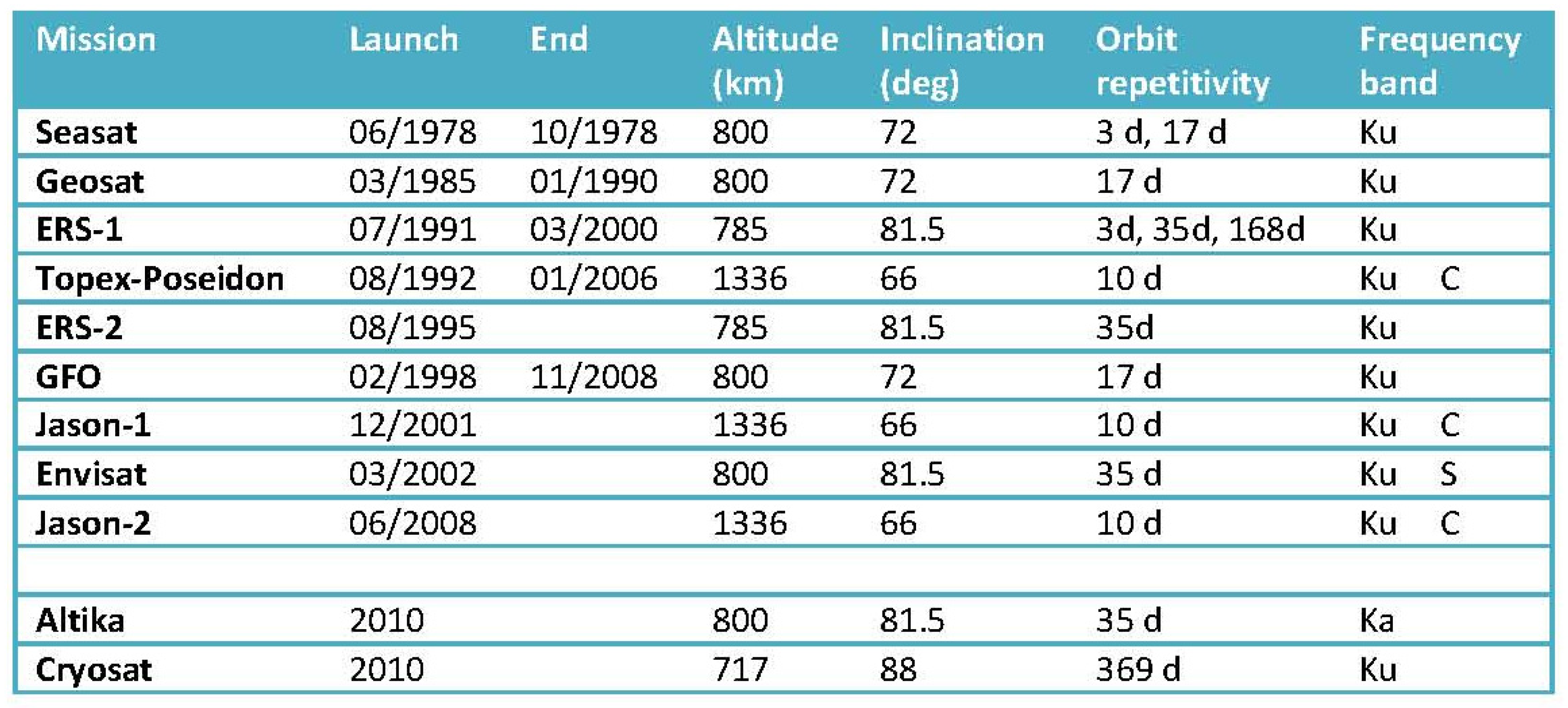
Altimetric missions with altitude, inclination, repetitivity and wavelength band (Ku, 13.6 GHz; C, 5.6 GHz; S, 3.2 GHz; Ka, 37 GHz) with respect to launch. Two future missions planned to be launched in 2010 are also indicated.
Table 1.
Altimetric missions with altitude, inclination, repetitivity and wavelength band (Ku, 13.6 GHz; C, 5.6 GHz; S, 3.2 GHz; Ka, 37 GHz) with respect to launch. Two future missions planned to be launched in 2010 are also indicated.

ERS-1, launched by the European Space Agency (ESA) in 1991, was the first polar-orbiting satellite with an altimeter onboard, it was followed by ERS-2 in 2005. Except for the small areas of the Greenland and of the Antarctic that have previously been observed with altimeters on-board Seasat, the ERS-1 observations are the first ones over large polar areas. The nominal ERS-1 orbit has a 35 day repeat cycle leading to a cross-track sampling of 15 km at latitude 70°S. ERS-1 has also flown with a 3 day repeat cycle and a so called “geodetic” (two 168-day repeat cycles shifted) orbit allowing a very dense sampling of the ice sheets (see Section 4.1). The measure is carried out at the 0.05 s frequency which corresponds to a 350 m spatial resolution along the satellite track.
In order to provide information for the ionospheric corrections above oceanic surfaces, altimeters have now a lower frequency added to the classical one in Ku band. The first dual-frequency altimeter (C and Ku-bands) was Topex-Poseidon launched in 1992 which was dedicated to oceanic studies.
The Envisat altimeter, launched in April 2002 is the first dual-frequency altimeter (S and Ku-bands) devoted to polar observations. It follows the same 35-day orbit as ERS-1 and ERS-2 to ensure a homogeneous time series.
3. Altimetric Waveform Shape, Surface and Subsurface Parameters
The main purpose of altimetry above ice sheet is the surface topography retrieval for ice dynamics study and for monitoring surface height variations. On one hand, it is of first importance to well understand how penetration of the radar wave within the snowpack affects the height measurements. On the other hand, some surface or snowpack characteristics may be retrieved from the waveform shape. This section is then devoted to the physics of altimetric measurements and will sum up some attempts to derive snow parameters from radar altimetry.
3.1. Relation between Waveform Shape and Geophysical Parameters
As already mentioned, the Ku-band wave (13.6 GHz) penetrates within the cold and dry snow medium, so that the reflection comes both from the surface and from the internal layers. The capacity of the wave to penetrate within the snowpack depends on snow dielectric properties. The absorption coefficient mainly depends on snowpack temperature [30] and the scattering coefficient mainly depends on snow grain size [31]. The surface backscattering depends on snow roughness but also on snow density [32,33]. The intensity of the internal backscatter depends on internal stratification [34,35] that in turn depends on snow accumulation rate. Thus altimetric waveform shape is sensitive to meteorological conditions close to the surface such as winds (through roughness), temperature (through grain size and density) or snowfall events (stratification and density). The main issue in altimetric measurements interpretation is to distinguish between all these effects.
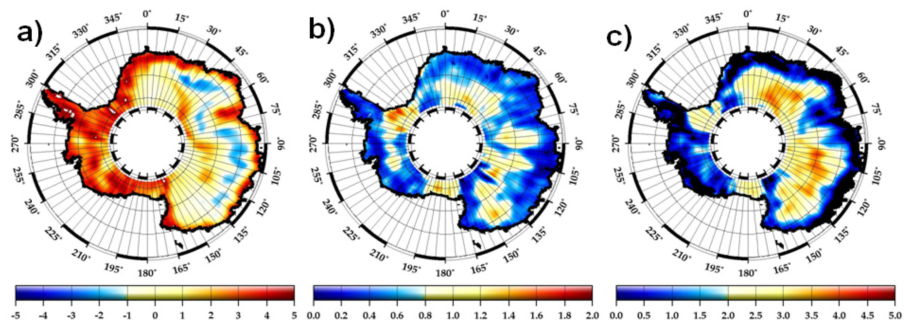
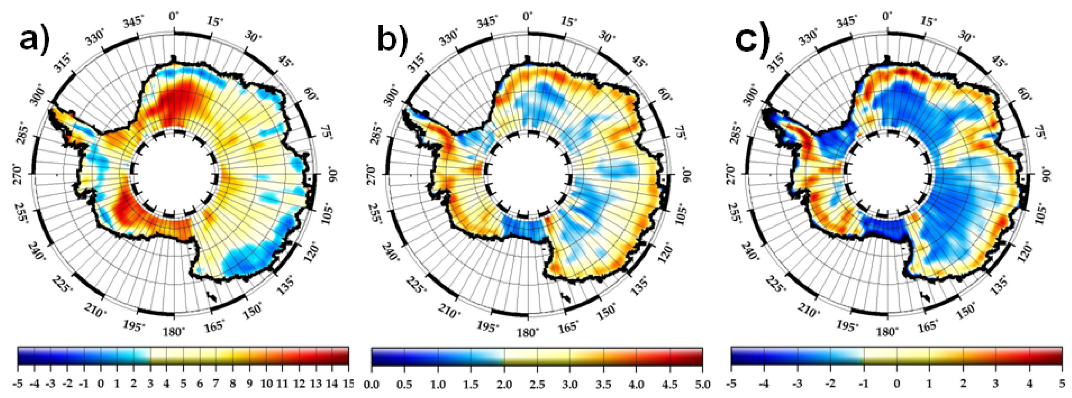
The three waveform parameters given by the ICE-2 retracker (Figure 3) are mapped on Figure 4. The range of variability of the parameters is important. The backscattering coefficient increases from −3 dB near the coast to more than 15 dB in the Dronning Maud Land area, e.g., it is multiplied by a factor of 100.
Several studies showed the impact of firn properties on the altimetric waveform [36,37,38]. They detailed which part of the waveform is mostly affected by the various surface and subsurface properties. Hence, the backscattering coefficient is controlled by both surface and volume echoes. Its amplitude is mostly influenced by surface roughness, snow stratification and extinction of the radar wave within the snow pack. The leading edge of the waveform is mostly controlled by the first echoes [39]. It is related to the surface roughness and to the first tens of centimetres of the subsurface [38]. On the contrary, the trailing edge part is mostly related to the ratio between volume echo and surface echo as well as the surface geometry. According to Davis and Zwally [39] the echo in East Antarctica is mostly dominated by volume signal whereas Lacroix et al. [40] pointed out the prevailing function of roughness. When surface is smooth compared to altimetric wavelength, volume signal is insignificant whereas for a rough surface volume signal highly modifies the waveform.
The penetration depth or the importance of volume signal can be empirically deduced from the altimeter, either by the analysis of the waveform shape [39] or by constraining a waveform model with the data from the 3-day orbit [41]. The first study [39] is dedicated to spatial changes of the extinction coefficient at the ice sheet scale. Due to increasing firn temperature from the high interior plateau toward the coast, grain size increases, and so does the extinction coefficient leading to shallower penetration depths. In the latter study it is assumed that on a temporal scale of 3 days, only surface echoes may significantly show variations, so that this study found a penetration depth varying from 12 m in the interior to 1 m near the coast.
Figure 4.
Mean altimetric waveform parameters mapped over Antarctica in Ku-band from 2003 to 2007. (a) The backscattering coefficient expressed in dB, (b) the leading edge width expressed in meters, (c) the trailing edge slope expressed in 106 s−1.
Figure 4.
Mean altimetric waveform parameters mapped over Antarctica in Ku-band from 2003 to 2007. (a) The backscattering coefficient expressed in dB, (b) the leading edge width expressed in meters, (c) the trailing edge slope expressed in 106 s−1.
Spatial variations of the volume signal are then very large at the ice sheet scale. For the first time, Davis [42] pointed out that besides these spatial variations, temporal variations of snow surface conditions could be high enough to alter the waveform and induce bias in the temporal height trends deduced from altimetric techniques. Temperature time series at the ice sheet scale are now long enough to constrain snow compaction model over ice sheets [43,44,45] and account for time variations of the volume signal. Indeed, firn densification processes [46] and rate of firn compaction have received increasing attention during the last decades since they are required for correct interpretation of elevation changes measured by satellite altimetry. Li and Zwally [45] used firn temperature time series from AVHRR infrared sensor for Antarctica back to 1982 to study height variations due to compaction from 1993 to 2003 and match their results with altimetric height measurements. They show that densification depends not only on the present temperature variations, but also on the past ones. Thanks to their model they manage to explain seasonal height variations of the ice sheet measured by satellite altimeter that were not consistent with changes due to snowfall. More recently, Helsen et al. [47] computed firn height variations in response to accumulation rate and temperature variability. They mentioned that enhanced accumulation obviously leads to firn thickening, but higher accumulation rates occur when temperature is higher than average, so densification is enhanced too and the total effect is diminished. Furthermore, Arthern and Wingham [43] modelled the impact of an increase in accumulation and found a change in density throughout the ice column as an immediate answer to that extra load followed later by a weaker rate of densification deeper in the column as if ice were already dense enough. The changes in height variations due to snowfall induce changes in density which alters the altimetric height retrieval and make it difficult to convert in ice mass changes. Taking into account snowfall variability Helsen et al. [47] showed that insignificant trends in accumulation could cause considerable ice sheet elevation changes, and found it necessary to take accumulation variability into account to accurately interpret ice sheet elevation changes. One can show that there is more than 10% chance of measuring an artificial trend greater than 15% of the mean accumulation rate from a 10-year elevation series and that the trend in mass and in volume can even be inversed [48].
3.2. Dual-Frequency Observations
Obviously, both the direct modelling of the waveform behaviour and the retrieval of snow parameters from waveform shape are difficult because the problem is under-constrained. The antenna gain pattern, the roughness sensitivity, the absorption and the extinction parameters are clearly frequency dependant so that dual-frequency information may improve our understanding of altimetry above snow.
A first attempt with the Topex-Poseidon altimeter operating in Ku and C-band (5.2 GHz) and covering the southern part of the Greenland ice sheet has confirmed the impact of the frequency on the altimetric measurements [49]. The authors showed that height differences are of a few decimeters only, and pointed out kilometric scale variations in the difference. The induced volume error seems to be also linked to the waveform deformation by surface topography [38]. The Envisat altimeter has operated in Ku and S-band (3.2 GHz) up to the end of 2007, unfortunately the S-band is out-of-order since January 2008. The lower frequency is then 4 times smaller than the Ku-band one. The difference between both bands is significantly larger than the noise: a few dB for the backscattering coefficient, a few meters for the leading edge and the height, a few millions 1/s for the trailing edge. Moreover, the corresponding maps exhibit a coherent signal [50]. Note that the altimeter is pulse limited meaning that the footprint size only depends on the pulse length (3 ns) and on the altitude, not on the frequency. The only frequency effect has been found on the height retrieval when surface slope is of the order of the antenna aperture.
Figure 5.
Difference in the altimetric waveform parameters between the Ku-band and the S-band, from the Envisat altimeter. (a) The backscattering coefficient expressed in dB, (b) the leading edge width expressed in meters, (c) the trailing edge slope expressed in 106 s−1.
Figure 5.
Difference in the altimetric waveform parameters between the Ku-band and the S-band, from the Envisat altimeter. (a) The backscattering coefficient expressed in dB, (b) the leading edge width expressed in meters, (c) the trailing edge slope expressed in 106 s−1.

These differences in the sensitivity of the two frequencies induce different spatial patterns of the waveform parameters. The range of variations of these differences is quite important and significant.
The three first reliable ENVISAT cycles were studied in Legresy et al. [50]. Spatial variations of the waveform shape in Ku and S bands are described. Surfaces are seen smoother at longer wavelength (meaning S band) as if long wavelengths could not see small scale features [40]. Surface signal is then stronger at longer wavelength. The same observation applies to grain size. This should be saying that snow grains scatter more strongly the closer they are in size to the radiation wavelength, i.e., Mie scattering. Therefore the S band signal penetrates deeper beneath the surface than the Ku band one. S band signal is thus more affected by a highly stratified medium. Another difference pointed by this study [49] is that due to the larger antenna aperture in S band, the corresponding signal is less affected by surface slope.
Figure 6.
Difference in altimetric height between the Ku-band and the S-band of the altimeter from [22]. This map illustrates very well the effect of the penetration of the radar wave within the snow pack because it depends on the wave frequency. This map can also be used to derive the principal characteristics of the snow pack and of the surface roughness.
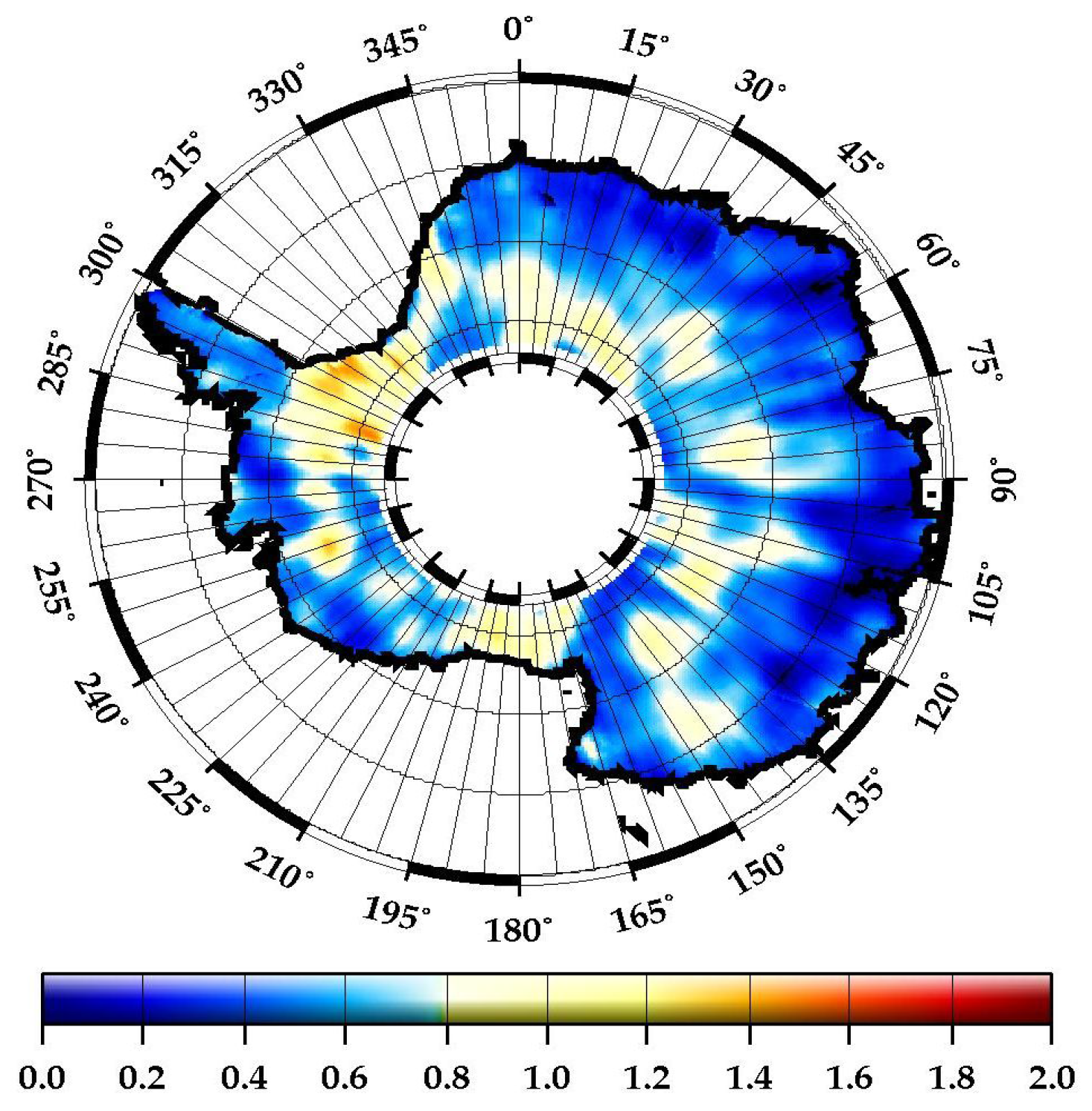
As an example, the difference in height is shown on Figure 6, it can reach up to 2 m in the central part of the plateau and above ice shelves. It is either attributable to different penetration depths or to different volume or surface echoes amplitude. This map illustrates very well both the kind of information offered by the dual-frequency altimeter and the difficulty to well extract the height from a microwave altimeter due to the penetration of the radar wave within the snow pack. S-band wave penetrate deeper so that the Ku-S difference is positive. However, the surface roughness is smoother in S-band and we may expect a greater surface echo. The opposite occurs on the plateau where the surface is smoother. We think that a larger quantity of internal reflected signal coming from the snow stratification explains this observation. First results confirmed that dual-frequency altimeter may be used as sounding radar. Above the large cracks of the Amery ice shelf, Ku-band sees very well the edge of the crevasses while S-band is sensitive to the snow deposited in the cracks [51]. A radiative model [40] has been developed to simulate the behaviour of the altimetric waveform with respect to snow parameters for the two-frequencies. Surface parameters are seen differently depending on the wavelength used for the survey. This model shows the high sensitivity of the measurements to surface roughness, especially in Ku band. In case of a smooth surface only, height measurements are reliable for mass balance monitoring. In one hand, when the surface is rough, the volume echo becomes too large and induces error in height retrievals. On the other hand, a high volume echo is interesting for instance to get information on the layering of the medium which is related to accumulation rate.
3.3. Toward the Restitution of Some Snow Parameters
The capacity of the radar altimeter, a nadir looking angle radar, to measure wave height from the leading edge [52] and surface roughness from the backscattering coefficient was exploited very early over oceanic surfaces [53,54]. Both of these information yield to wind speed retrieval over oceans [55].
As for oceanic surface where wind induces two roughness scales (micro-roughness and waves), katabatic winds carve the ice sheet surface at the centimetric scale (micro-roughness) and at the metric scale (sastrugis or erosional snow features) [56] so that they control the microwave emission and backscatter [57]. As for the oceanic case, the altimetric backscattering coefficient is indeed sensitive to wind intensity [37]. This study, with the help of the Seasat data, points out the strong relation between katabatic wind intensity and backscatter variations. Winds are indeed responsible for the presence of snow features on the surface such as sastrugi, and changes in surface roughness. They obtained a local relationship that can hardly be extrapolated to the whole ice sheet. Indeed, correlations between wind variations and selected altimetric waveform parameters can be surprisingly high, but with spatial pattern which highlight localised interaction between wind and surface state.
The use of not only the backscattering coefficient but also the whole information contained in the waveform, to retrieve surface and subsurface properties of the snow medium was also performed with the Seasat altimeter [28,36]. The latter study noticed that some changes in the waveform can have several causes that could hardly be distinguished. For instance snow grain size and snow density may produce the same waveform changes. Volume signal and surface topography might have opposite effect on the leading edge and the analysis of the first part of the waveform only is not sufficient to detect surface and subsurface properties [50]. Indeed, similar waveforms may be obtained with different subsurface combination of properties [25]. On the contrary, different waveforms may be obtained with the same volume contribution but with different local topographies [38].
The study of the space and time variations of the altimetric waveform highlighted strong seasonal variations of all the three waveform parameters, with the backscatter maximum occurring at the time of the leading edge width and trailing edge slope minimum, and varying depending on the location on the ice sheet. Seasonal snow densification processes are probably the best candidates to explain the observed seasonal cycles in the waveform [51].
Retrieving stratification is a tricky issue. Swift et al. [58] reported that buried layers are a significant source of additional backscatter. The overall waveform is affected by snow layering, and the effect is not the same depending on how deep the layer is [59]. Stratification is highly related to accumulation rates, and the sensitivity of the altimeter to the depth of internal layers, especially in Ku band for low accumulation area [40] may help to retrieve accumulation pattern on the highly stratified plateau only.
A tentative to invert the surface properties of ice sheets from satellite microwave data in order to correct altimetry errors has been performed over the Greenland ice sheet [60]. The objective was to assess the impact of interannual variability in accumulation rate on the rate of elevation changes as measured by the altimeter. This work suggests that such a technique could be applied when a more extensive validation will be performed. However, the interannual variability in accumulation rate is less in Antarctica than in Greenland but such a technique may be of interest in the future.
To finish, one of the problems in attempting to retrieve snow parameters is the lack of in situ measurements at the global scale. Up to snow in situ measurements are obtained either near stations (mostly in the coastal areas) or along few raids during the austral summer. Besides that, pertinent parameters for altimetry (surface roughness or snowpack parameters gradient) are up to now very difficult to measure. A new methodology to measure snow surface roughness with a laser has recently been tested in Svalbard [61]. Such measurements are actually tested at Dome C in Antarctica so that validation of the surface roughness retrieval by altimetry will be soon possible. However most of the attempts to invert electromagnetical models [28,35,39,40,45] find snow parameters in a suitable range.
4. Application of Radar Altimetry for Ice Sheet Dynamics Study
4.1. Construction and Precision of the Derived Topography
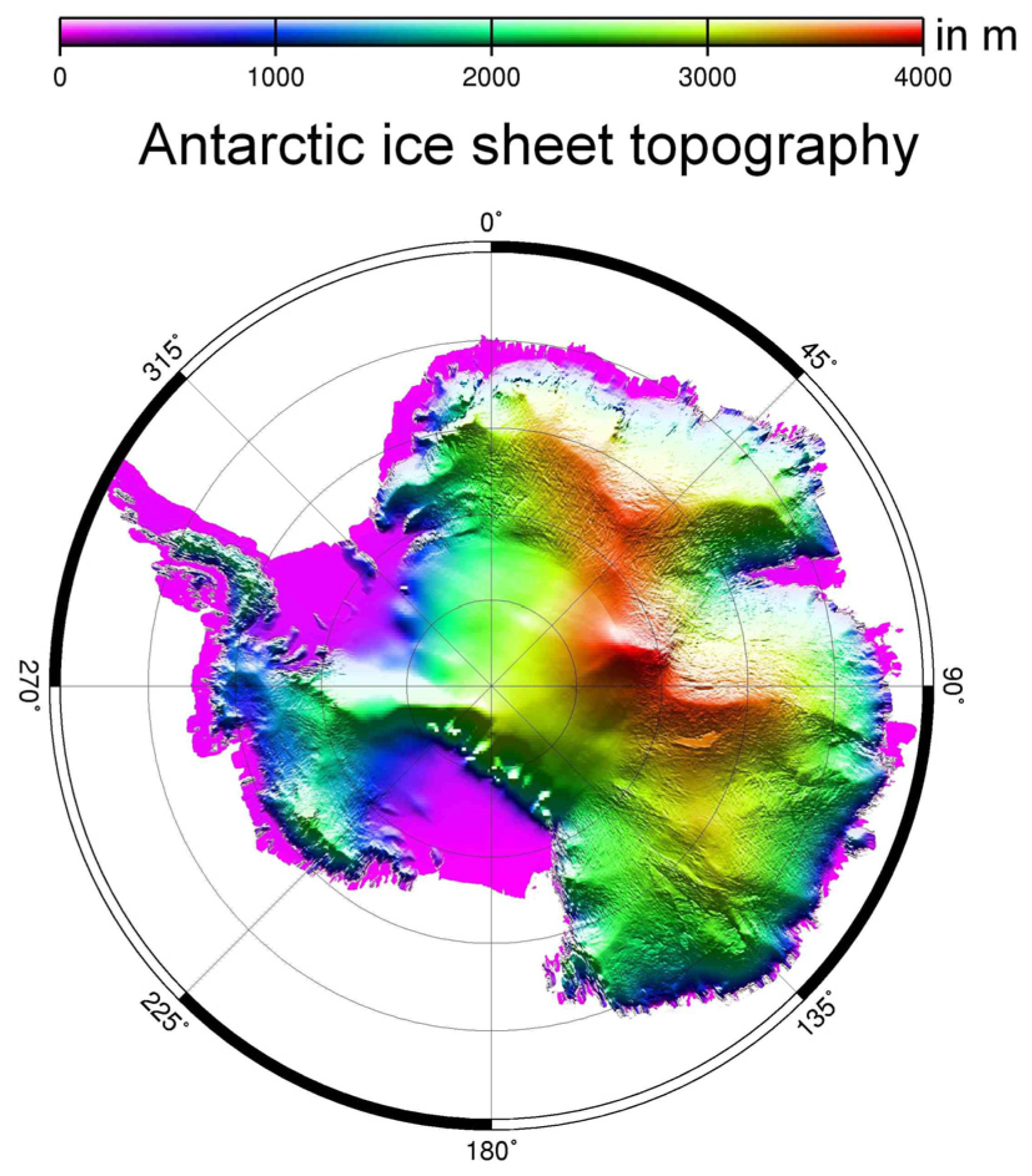
Accurate information of the ice sheet topography is crucial both for ice dynamics studies and for the prediction of the future evolution of ice sheet. From April 1994 to March 1995, ERS-1 was placed on a geodetic orbit (two shifted cycles of 168-day repeat). The satellite track sampling is 10 times greater than in the 35-day orbit leading to a cross-track distance of 1.5 km at latitude 70°S. Up to 30 million waveforms were collected and reprocessed over Antarctica. Data editing and geophysical corrections were taken from [62]. The small-scale topography signal yielded to a poor on-board tracking of the ground, that was corrected by using a dedicated retracking algorithm previously developed [25,38]. The Delft Institute precise orbit is used and the altitude is given with respect to the WGS-84 ellipsoid with a grid size of 1/30°. As shown in Figure 3, this high-resolution topography reveals numerous details from the kilometric to the global scale that we will comment in the next subsection.
The laser altimeter IceSat launched in 2003 [63] is less sensitive to ice penetration and is less to surface slope than the radars, it then allows finer analysis to be performed. The bias between Envisat and IceSat increases from −0.40 m ± 0.9 m for surface slope lower than 0.1 degree to 0.05 m ± 26 m near the coast. The mean difference is around 0 because of the effects of penetration and residual slope error are opposite. Note that the root mean square (r.m.s) strongly increases from inside regions to the coast [20,64]. The same kind of results are obtained using comparisons with GPS data in some places [65].
Roemer et al. [19] performed a finer analysis of radar altimetric data in the vicinity of the Vostok lake. They developed new techniques to correct for topographically induced errors and improved the gridding procedure. They improved the precision from 1 m with previous techniques to 0.5 m and pointed out the smoothing of the topography made by radar altimeters that prevents from detecting the small scale topographic features.
4.2. Ice Dynamics Information Derived from Topographic Signatures
The main physical processes (climatic and dynamic) that act on an ice sheet induce particular signatures on its free surface. From the small scales to the larger ones, topography contains important information on local anomalies or on general trend behaviours [11,62]. Accurate knowledge of the topography also provides a current initial condition to analyse its future evolution. At the large scale, the surface is quasi-parabolic and governed by ice viscosity and by flow boundary conditions. The topography is mostly controlled by the distance to the coast [66,67], except where basal conditions, such as sliding, affect the topography in the upslope direction [67]. The large scale topography controls flow direction and its mapping allows calculating balance velocities (see Section 4.3).
At this large scale, networks of anomalies of the surface topography perpendicularly to the greatest slope direction can be pointed out. They are due to boundary flow conditions of outlet glaciers that are propagated from the coast up to the dome [68]. It exhibits the drainage pattern, upstream glacier positions or the flowline directions, but also the role of the outlet flow conditions on the whole shape.
At the 10-km scale, topographic signatures of the flat ice shelf enable to delimit adjacent glaciers and to visualize lateral stress effects. “En echelon” structures with a tilted orientation of 45° with respect to the flow direction are found and not yet well explained [62].
In the same way, undulations at the 10 km scale wavelength with a metric scale amplitude seem to be the main ice sheet surface features. They have been early attributed to ice flow above an irregular bedrock [69,70]. Up to now, they are modelled as symmetrical dome shaped features. Their spatial characteristics may allow a better understanding and modelling of these structures: they are found to be elongated with a frequent orientation of 45° with respect to flow-line directions. The 10 km scale seems to be a characteristic scale of ice flow processes, as we will see in the next subsection.
Figure 7.
High-resolution map of the Antarctic Ice Sheet topography from the ERS-1 geodetic mission [7]. The elevation reaches 4000 m. Note the numerous details: ice shelves surrounding most of the continent, surface undulations, flat areas reflecting subglacial lakes, elongated scars due to hydrological networks.

4.3. Subglacial Lakes and Hydrological Networks
In the early 1950s ice penetrating radio-echo sounding revealed the existence of subglacial lakes in Antarctica [71,72]. The presence of basal water below the ice induces sliding that in turn induces a flat and smooth signature on the ice sheet surface. The altimeter is then an efficient tool for detecting subglacial lakes. Since the launch of ERS-1 that allows the first description of the greatest lake, the Vostok lake [73], few tens of lakes have been discovered [74,75,76] so that actually up to 150 lakes are known and many of them have an activity (drainage/filling). The presence of lakes is now recognized to be an important factor in ice dynamics and even in some case to play a role in ice streams behaviour [77,78,79,80].
With a precise topography analysis one can observe that these local sliding areas are surrounded by two symmetrical topographic anomalies. These bumps and troughs on the topography are associated to abrupt transition, respectively from weak friction (in case of sliding) to strong friction (in case of deformation) and inversely from strong to weak friction. One can show that these transitions occur on two steps, longitudinal extension followed by longitudinal compression for a transition between deformation and sliding, and inversely [62]. The characteristic scale of the longitudinal variations, and thus of the longitudinal stress, is thus about 10 km.
Thanks to the particular signature of lakes on the surface one can detect local anomalies related to basal water. A dedicated methodology based on the estimation of the surface curvature allows enhancing subtle surface features observed in the ice sheet surface topography so that several elongated networks have been identified and related to subglacial topography in the vicinity of Dome C [81]. At the ice sheet scale, one can detect hydrological systems which cross the continent over distances greater than a few hundred of kilometres [82]. Some of these features are connected to the ice-sheet margin, although the low number of such features means that transportation of subglacial melt water within these channels does not significantly contribute to ice sheet mass loss at the continental scale. However their influences on outlet glacier flow will be discussed in Section 5.
4.4. Balance Velocity and Ice Dynamics
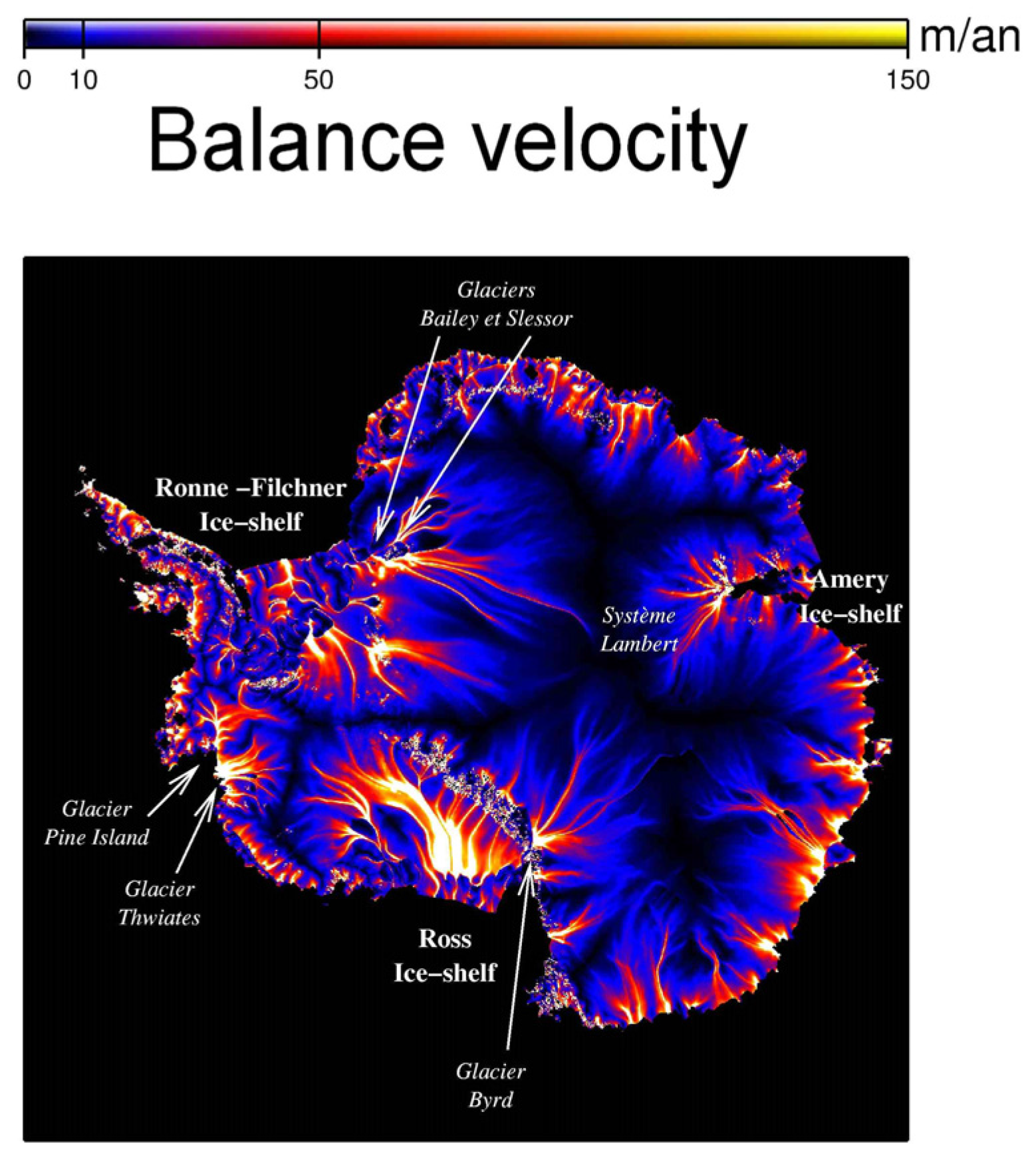
The ice flow follows the down-slope direction so that the topography provides the direction of the ice flow and the convergence or divergence of flow-lines. The summation of the accumulation rate from the dome to the coast between two flow channels makes it possible to estimate the ice flux, by stating that the flows coming in and out of an ice column are equal. Velocity is obtained by dividing by the ice thickness from BEDMAP experiment [83]. To do this, we have to assume that the ice sheet is in balance, so that this velocity is called the balance velocity [84].
Balance velocity (Figure 9) is lower than 1 m/yr near the dome and reaches 100 m/yr near the coast [85,86]. It is clear that ice flow divergence and convergence are controlled by the surface topography that plays a significant role in ice flow. One can observe fast flowlines or ice streams, with tributaries networks, whose effects are felt until several hundred of kilometres inside the continent. Indeed, 80% of the continent is found to be drained by only 20% of the coast. It is probably one of the major discoveries provided by altimetry for Antarctica. Indeed, this irregular flow distribution/ice flow network gets important consequences concerning ice sheet behaviour regarding to climate change. A fast glacier will respond more quickly to perturbations than a slower one. Also, a perturbation at the coast, for instance a change in the velocity of an outlet glacier, will propagate all along the stream. It then highlights the most sensitive areas of the ice sheet.
Figure 8.
Map of the balance velocity expressed in m/yr from [15]. Note the presence of numerous ice streams that can be followed far away in the upslope direction. The name and location of the main outlet glaciers are shown.
Figure 8.
Map of the balance velocity expressed in m/yr from [15]. Note the presence of numerous ice streams that can be followed far away in the upslope direction. The name and location of the main outlet glaciers are shown.
The surface topography also gives indications on the dominant stress that acts on ice deformation, the so-called basal shear stress related to the surface slope. The deformation velocity depends on the basal shear stress via the rheological parameters that are the main unknowns of ice sheet dynamics [87]. The first attempt to use velocity and stress derived from topography to better constrain the rheological parameters was done by Young et al. [88] with the help of the topography from Zwally et al. [29]. They found constant values for rheological parameters. By taking into account the ice temperature, one can show that rheological parameters depend on the velocity range so that the ice is a fluid with a non linear viscosity [89]. Finally, Testut et al. [90] showed that too many parameters were affecting the flow (sliding, anisotropy, longitudinal stress), so that further studies, based on topography alone, would be unsuccessful for retrieving ice sheet rheological parameters. Recent studies now use the topography to constrain model and, for instance, to improve ice core dating [91,92].
Eventually, the balance velocity compared with velocity derived from an independent technique, may, in theory, help to estimate the ice sheet mass balance. If the observed velocity is larger than the balance one, the ice sheet wastes mass. Unfortunately, the poor knowledge of the accumulation rate required to estimate the balance velocity results in a lack of robustness of such a technique at the global scale. The ice sheet mass balance can only be computed thanks to this technique if the snow accumulation rate is well known over the drainage basin. For instance, it has been suggested that the discharge flux over the Mertz basin was too low to compensate for the snow supply through accumulation (lower than the accumulation rate) so that this sector may be in a positive imbalance [93]. However, the authors also pointed out that large errors in the accumulation maps impede reaching a firm conclusion about the Mertz mass balance [93]. Similarly, Fricker et al. [94] showed that for the Lambert Glacier and Amery ice shelf system the poor knowledge of accumulation rate over the drainage basin prevents from applying such a technique.
Nevertheless, mass balance may be estimated directly with topographic survey as we will see in the next section.
5. Ice Sheet Mass Balance
5.1. Methodology and Error Budget
As mentioned in the Introduction, it is not easy to determine mass balance because of our lack of knowledge of the physical processes affecting both ice dynamics and polar climate. Even surface mass balance depends on several different mechanism that are not easy to predict [95]. Recent general reviews of the different remote sensing techniques to derive ice sheet mass balance can be found in Bamber and Rivera [96] or in Remy and Frezzotti [7]. Three different ways of estimating mass balance exist: measuring the difference between input and output, monitoring both the ice fluxes and the climatic evolution, or directly monitoring the volume shape. Optimal method combining different data from ice budget or geodetic approach are found to be more efficient [97] but are not frequently used. It is now clear that time series obtained by radar altimetry are long enough to address the problem with the third way. Moreover, the spatial resolution of altimetric data compared with other sensors such as gravimetry allows catching some small-scale feature changes linked with specific processes.
Several attempts to derive ice sheet mass balance with the help of the altimetric time series of ERS-1, ERS-2 and Envisat have been published [98,99,100,101]. The whole details of the data processing can be found in each of these papers. In order to derive height variation trends, most of the methodology focuses on the difference at cross-over points in order to minimize long-scale errors and the error due to the antenna polarization [102]. Only one study [100] uses repeat tracks, leading to larger data sets with a finer resolution.
However, one has to keep in mind that the error budget is important in space and also in time due to the penetration error that is highly variable. Despite the different corrections proposed by the authors, the final error might be important. Also, as already mentioned in Section 3.1, the snow densification is also a problem that acts both directly on the volume and indirectly because of its impact on the waveform shape and thus on the height retrieval. It is one of the explanations of the difference between altimetry (that measures volume) and gravimetry (that measures mass) as we will see in the next section.
In order to correct for the previously mentioned errors we fit a 12-parameter function to the time series at each along-track position. Without going into the details, we take into account the surface slope at the medium scale by fitting a bi-quadratic form (6 parameters), we take into account the effect of the temporal changes in the snow pack characteristics by fitting a linear relation with the three waveform shape parameters, we remove the seasonal variability with a sinusoidal function (amplitude and phase or fit a sine and a cosine) and to derive the trend we add a linear relation with time. The drift of the tracks being within one kilometre, we consider altimetric data over a radius of one kilometre along and across the mean track, leading to around three observations for each cycle. The precision of the fit increases with time series length. With a 4-yr time series the fit is constrained by 120 measurements, enough to constrain the 12 parameters. One can show that the fit of the stationary parameters is convergent as soon we own around 40 cycles.
To finish, it should be noted that the inability of altimeter to resolve ice sheet margins is negligible because of the weak percentage of margins (even weighted by snow accumulation rate) with respect to the whole ice sheet surface. We will first focus on the regional scales and will finish with surveys at the global scale.
5.2. Monitoring the Small Scale Features
Due to the inertia of processes acting on ice sheet mass balance (see Figure 1), one may assume that surface mass balance mechanics are the main factors at the decadal scale. However, altimetry monitoring points out that some surface changes indubitably linked with dynamics processes, in particular changes at the scale of tens of kilometres. We do not want to review here all the papers dealing with small scale features monitoring by altimetry, but just want to highlight someimportant discoveries.
One of the most interesting and surprising processes discovered thanks to the radar altimetric time series is the rapid discharge of subglacial lakes [103]. These authors measure a transfer of 1.8 km3 of water from one subglacial lake toward two other lakes 290 km away. Since then the fact that such subglacial drainage systems may have impacts on ice flow and on mass balance became more and more obvious. Indeed, another rapid discharge of 2 km3 from one subglacial lake, in the western part, directly to the ocean have been first observed [78]. Later, in the eastern part, a discharge of about 1.7 km3 of water from a large subglacial lake in the upslope direction of the Byrd glacier has coincided with an acceleration of the glacier [104]. The influence of subglacial water discharge on ice flow velocity is now an important issue. It depends on a few parameters such as the volume of the discharge or the geometry of the emissary basin. The problem is not so much the induced water mass loss, but the water pressure increase that may enhance the ice flow velocity [105].
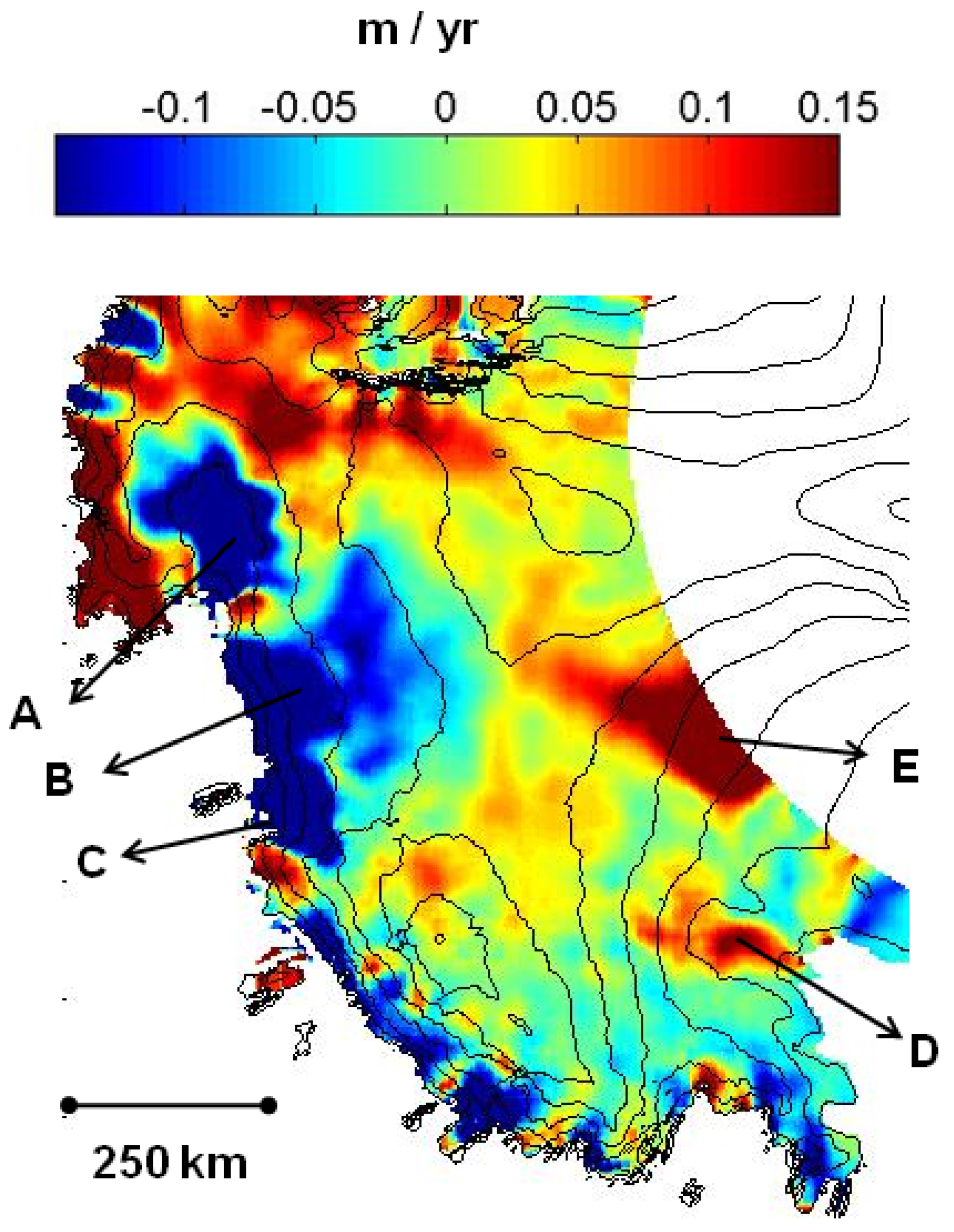
Another surprising finding was the detection of rapid change in the volume of several outlet glaciers. The most famous ones are the space and time evolutions of the glaciers belonging to the Amundsen Sea drainage systems (Pine Island, Thwaites and Smith Glaciers). With the help of radar altimetry and interferometry, Shepherd et al. [106,107] showed that the rapid thinning of ice was detected up to 150 km inland. The three mentioned glaciers thinned by more than 1.6, 2.5 and 4.5 m at the ground line location between 1992 and 1999, respectively, and while the Thwaites and Smith glaciers increased by 25 and 45 m between 1991 and 2001, respectively. The signature of this thinning suggested a dynamical answer of the ice initially due to ocean thermal forcing. Indeed, the thinning rate decreases with distance to the coast. An outlet perturbation is then clearly propagating in the upslope direction. The imbalance of this sector is sufficient to raise sea level by more the 0.2 mm/yr [108]. The latest studies on the Pine Island glacier confirm the inland thinning and its relation with internal dynamical processes [109]. The grounding line retreat toward the interior is such that the main part of the glacier might be afloat within the next century [110]. However, in the same sector, some glaciers are also found to be thickening, as shown on Figure 9.
The same is also observed on several ice shelves that are often found to be thinning. For instance, altimeter observations from 1992 to 2001 over the Larsen ice shelf suggested a thinning of 0.27 m/yr [111]. Now, longer time series analysis, for instance over the Amery ice shelf, exhibit short-term fluctuations so that one cannot conclude that short time period signal necessarily indicates ice shelf instability [112].
5.3. Monitoring Antarctic Ice Sheet at the Global Scale
The mass balance for the Antarctic ice sheet at the global scale is mapped on Figure 9 and is borrowed from this last study. The behaviour of the West and East part are quite different. The West Antarctic ice sheet is a marine ice sheet, since most of its bedrock is under sea level. Firstly, it is thus very sensitive to an increase in oceanic temperature. Secondly, it gets a relatively higher geothermal flux than the Eastern part, meaning that basal temperature is larger [113]. As a consequence most of the ice lying on the bedrock gets a temperature close to the melting point and the ice slides down at higher velocity. Thirdly, the west Antarctic dynamics depends on a complex network of fast tributaries ice stream. These glaciers quickly respond to a climate change. This sector exhibits volume fluctuations over a large range of timescales. Mass balance observations support the different behaviour between these two parts.
Figure 9.
Enlargement of the changes in height in the west Antarctic ice sheet during the period 2002–2008. The Pine Island, Thwaites and Smith Glaciers sectors (noted A, B, C) decrease at a rate greater than −0.15 m/yr while other glaciers (D or E) increase during this period. D is found to thinning only during the Envisat period, this shows that the upslope signal is propagated in few years over several hundred kilometres. E corresponds to the upslope part of the Kamb ice stream that flows out of the Envisat coverage. Its thinning up to the coast is confirmed with the IceSat data [114].

All attempts to derive mass balance from altimetry agree with a clear thinning of the draining basin of the Pine Island and Thwaites glaciers, in the western part of the WAIS (see Figure 4). One of the authors found a thinning of the whole West Antarctica at a rate of 47 Gt/yr [98] corresponding to 0.12 mm/yr of sea level rise. Another one detected dynamic responses of the WAIS leading to either thickening or thinning [99]. Finally, Legrésy et al. [100] used a different methodology to extract the temporal trend by correcting for the penetration with the help of the backscattering coefficient and the whole waveform shape. They detected few areas of thickening, in the East part of Wilkins land or in the Peninsula and few areas of thinning, near the Pine Island sector or near Law Dome. Most changes in ice surface near the coast are attributed to change in ice dynamics due to perturbation of the outlet glaciers as previously explained. Most of the studies pointed out a local increase in accumulation rate in few areas, namely in the Peninsula, Dronning Maud land and East Wilkins part. In average, the studies found a signal comprised between 0.1 mm/yr and −0.1 mm/yr in term of sea level change. This signal, for all the different studies, is then found not to be statistically significant. On the contrary, the Eastern part seems to be more stable. Depending on the kind of corrections made, especially to account for penetration issues, various authors find this part to be slightly thinning or slightly thickening.
Depending on the technique (altimeter or gravimetry) and on the used methodology the western part is found to loss mass between −50 to −150 Gt and the Eastern part is found to gain mass between 0 to 60 Gt [115]. However, the comparison between the mass balance derived from ERS and Envisat for two different periods (see Figure 10) suggests that the strong temporal variability also explains a large part of the discrepancy, each study dealing with a different period. Note that we applied the same corrections to the ERS and Envisat data set to compare. Also the instrumental biases are removed because we compare directly each trend.
Figure 10.
Mass balance of the Antarctic ice sheet (in m/yr) updated from [18], for the ERS period (1992-2003) and the Envisat period (2002-2006). Note the important thinning of the West Antarctic ice sheet over a large sector. The Eastern part of the continent exhibits less impressive signals, but is also shown local fluctuations that depend on the period.
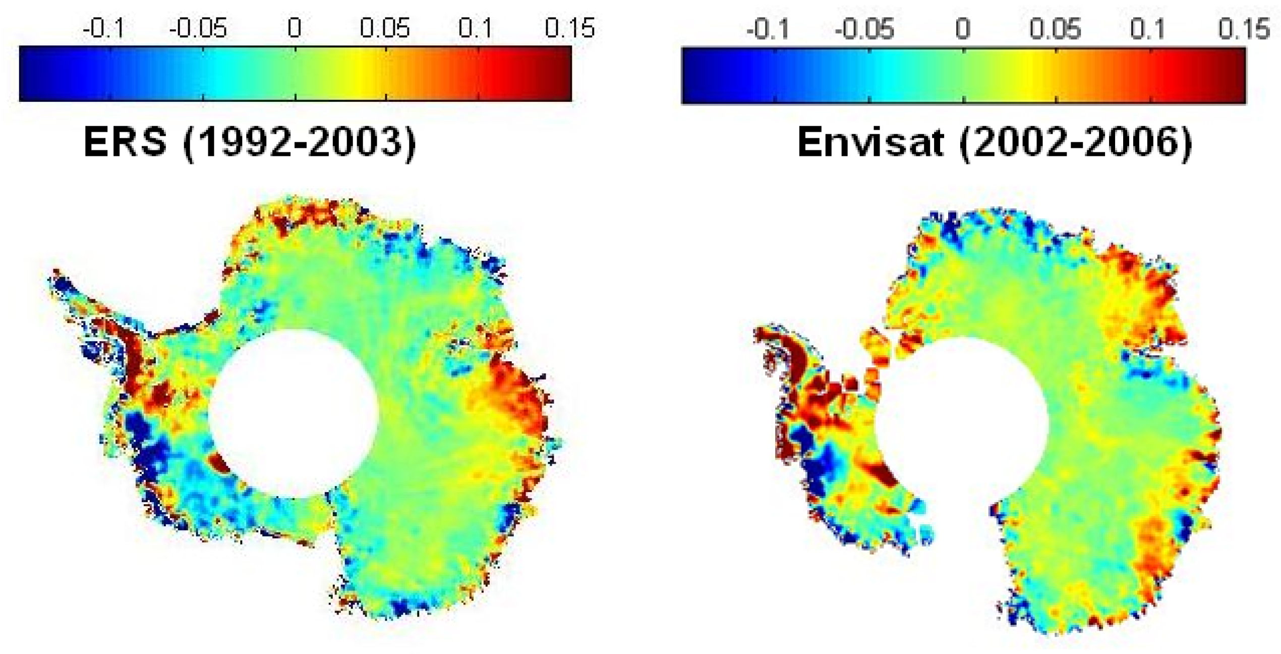
The amplitude of local fluctuations can be as large as 15 cm/yr (Figure 9) and are attributed to small temporal changes in precipitation [7]. The difference between both maps gets the same ranges of variations of the average map, meaning that more than 50% of the signal is not constant in time. Indeed, one can see the difference of the changes pattern between the ERS and the Envisat period. As soon as the distance to the coast is greater than 200 km, the amplitude of the variations falls down to a few centimetres per year. The centre of the East Antarctic ice sheet is then stationary over a few thousand kilometres.
However, our classical vision of two different parts in Antarctica in response to climate change is now altered because of recent observations. For instance, Shepherd and Wingham [116] showed with the ERS and Envisat time series that only glaciers that seat in submarine basins with no substantial ice shelf barrier are losing mass today and that such glaciers are situated in both parts of the Antarctica. Also, no global increase is observed so that the classical and intuitive idea of a gain in mass due to an enhancement of accumulation rate in a warmer climate seems to not be observed.
To sum up Antarctica happens to be close to equilibrium but strong regional signals suggest that local dynamical response of ice may accelerate in the future. Glaciers of both the East and West Antarctica may provide a substantial contribution to global sea level change [116]. Not only the altimeter is a useful tool to map global trends but it is also able to catch some local imbalance. However, some discrepancies between studies in some places may be explained by the limitation of retrieving height variations due to the penetration of the altimetric radar wave in the snow pack. Such effect has been pointed out in the Amery ice shelf [112]. Densification processes yield also to critical error because it directly acts on the height surface and indirectly via change in snowpack characteristics. For some authors, the magnitudes of firn depth changes are comparable to those of observed ice sheet elevation change [47].
6. Conclusions
The Seasat and Geosat missions have revealed the altimeter to be powerful tool for oceanic analysis. Whilst only the south of Greenland and a small portion of the Antarctic ice sheet were covered, (South of 72N and North of 72S), the missions also demonstrated the potential of altimetry for ice sheet studies. This led to the design of the ERS altimeter, with an orbital inclination and tracking capability to study ice surfaces. As a consequence satellite radar altimetry has become one of the most significant tools to enhance our knowledge of ice sheet characteristics. Almost 20 years of continuous observations, have allowed us to address important questions on ice dynamics, snowpack characteristics and ice sheet mass balance.
The precise description of the ice sheet surface has led to the determination of basin scale balance velocities through ice sheet dynamics. This has led to an improved model description of ice sheet stresses. Numerous subglacial lakes have been discovered along with interlinking hydrological networks. Thinning, several hundred kilometres upstream of accelerating glaciers has been detected, spurring the development of new processes in ice sheet models. We have shown that many surface features, identified in the altimetric waveforms, remain a mystery. For example, what are the relationships between winds and the surface undulations?
With the exception of the steep marginal zones where the measurement error is high, and the orbital limit (81.5º), the topography of both ice sheets is now well mapped. Optical stereo sensors have been used to map the ice sheet margins [117] but their sampling is incomplete due to clouds. In this context, the new ESA satellite Cryosat-2, dedicated to survey ice [118], will provide valuable data over the areas currently excluded from observations by radar altimetry.
Twenty years of altimetry have shown that the Antarctic mass balance is near neutral, and consequently the ice has no impact on global sea level change. However, there is no doubt that tidewater glaciers in the WAIS are causing a thinning and regional mass loss. Some regional trends are highly variable and further investigations are required to understand there changes. It is possible that these are related to changes in the penetration of the altimeter pulse into the snow pack. A recent analysis of Thomas et al. [119] over the Greenland ice sheet shows that the surface imbalance as measured by radar altimeter is more positive than the one measured by laser altimeter. The surface elevation bias between laser and radar altimetry varies spatially and temporally, the understanding of which would require independent surveys.
In the absence of such surveys, it may be possible to understand some of the differences through analysis of the S-band data from the dual-frequency altimeter on Envisat. Dual-frequency altimeters haves already demonstrated their potential for the lake-ice characteristics [120] and the estimation of snow pack thickness [121]. Preliminary work using dual-frequency observations over Antarctica indicate an ability to separate surface and volume signals, and consequently to derive parameters such as snow grain size and surface roughness.
There is a powerful case for continuity in altimetric observations, for accurate and timely cross-calibration between different missions and for in-situ validation of the different techniques. The launch of Cryosat-2 by ESA will increase our understanding of the time evolution of the ice sheets and extend the topographic map coastwards. Nevertheless, to ensure a perfect continuity of the observations, an Envisat follow-on mission with exactly the same technical and orbital characteristics is needed.
Acknowledgments
The authors are grateful to Fabien Blarel (Legos/OMP) for this help in data processing, Benoît Legrésy (Legos/OMP) for his discussion, help and data analysis and Etienne Berthier (Legos/OMP), Martin Horwath (Legos/OMP) and Alexei Kouraev (Legos/OMP) for their comments. We also thank the two anonymous referees for their numerous comments that greatly improve the manuscript.
References and Notes
- Meier, M.F. Ice, climate, and sea level: do we know what is happening? In Ice in the Climate System; Peltier, W.R., Ed.; Springer-Verlag, NATO ASI Series: Berlin, Germany, 1993; Volume 1-12, pp. 141–160. [Google Scholar]
- Paterson, W.S.B. The Physics of the Glacier, 3rd ed.; Butterworth-Heineman-Oxford Press: London, UK, 1994; p. 480. [Google Scholar]
- Vaughan, D.G.; Bamber, J.L.; Giovinetto, M.; Russell, J.; Cooper, A.P.R. Reassessment of net surface mass balance in Antarctica. J. Climate 1999, 12, 933–946. [Google Scholar] [CrossRef]
- Jouzel, J.; Masson-Delmotte, V.; Cattani, O.; Dreyfus, G.; Falourd, S.; Hoffmann, G.; Minster, B.; Nouet, J.; Barnola, J.M.; Chappellaz, J.; Fischer, H.; Gallet, J.C.; Johnsen, S.; Leuenberger, M.; Loulergue, L.; Luethi, D.; Oerter, H.; Parrenin, F.; Raisbeck, G.; Raynaud, D.; Schilt, A.; Schwander, J.; Selmo, E.; Souchez, R.; Spahni, R.; Stauffer, B.; Steffensen, J.P.; Stenni, B.; Stocker, T.F.; Tison, J.L.; Werner, M.; Wolff, E.W. Orbital and millennial Antarctic climate variability over the past 800,000 years. Science 2007, 317, 793–796. [Google Scholar] [CrossRef] [PubMed] [Green Version]
- Eisen, O.; Frezzotti, M.; Genthon, C.; Isaksson, E.; Magand, O.; van den Broeke, M.R.; Dixon, D.A.; Ekaykin, A.; Holmlund, P.; Kameda, T.; Karlof, L.; Kaspari, S.; Lipenkov, V.Y.; Oerter, H.; Takahashi, S.; Vaughan, D.G. Ground-based measurements of spatial and temporal variability of snow accumulation in east Antarctica. Rev. Geophys. 2008, 46, 1–39. [Google Scholar] [CrossRef]
- Frezzotti, M.; Pourchet, M.; Flora, O.; Gandolfi, S.; Gay, M.; Urbini, S.; Vincent, C.; Becagli, S.; Gragnani, R.; Proposito, M.; Severi, M.; Traversi, R.; Udisti, R.; Fily, M. Spatial and temporal variability of snow accumulation in East Antarctica from traverse data. J. Glaciol. 2005, 51, 113–124. [Google Scholar] [CrossRef]
- Remy, F.; Frezzotti, M. Antarctica ice sheet mass balance. C. R. Geosci. 2006, 338, 1084–1097. [Google Scholar] [CrossRef]
- Cavalieri, D.J.; Parkinson, C.L. Antarctic sea ice variability and trends, 1979-2006. J. Geophys. Res.-Oceans 2008, 113, 1084–1097. [Google Scholar] [CrossRef]
- Bindschadler, R. Monitoring ice sheet behavior from space. Rev. Geophys. 1998, 36, 79–104. [Google Scholar] [CrossRef]
- Masson, R.; Lubin, D. Polar Remote Sensing; Springer: Berlin, Germany, 2006; p. 426. [Google Scholar]
- Kerr, A. Topography, climate and ice masses—a review. Terra Nova 1993, 5, 332–342. [Google Scholar] [CrossRef]
- Remy, F.; Legresy, B.; Testut, L. Ice sheet and satellite altimetry. Surv. Geophys. 2001, 22, 1–29. [Google Scholar] [CrossRef]
- Fu, L.L.; Cazenave, A. Satellite Altimetry and Earth Sciences: A Handbook of Techniques and Applications; Academic Press: San Diego, CA, USA, 2001. [Google Scholar]
- Fu, L.L.; Christensen, E.J.; Yamarone, C.A.; Lefebvre, M.; Menard, Y.; Dorrer, M.; Escudier, P. Topex/poseidon mission overview. J. Geophys Res.-Oceans 1994, 99, 24369–24381. [Google Scholar] [CrossRef]
- Cazenave, A.; Schaeffer, P.; Berge, M.; Brossier, C.; Dominh, K.; Gennero, M.C. High-resolution mean sea surface computed with altimeter data of ERS-1 (geodetic mission) and Topex-Poseidon. Geophys. J. Int. 1996, 125, 696–704. [Google Scholar] [CrossRef]
- Cazenave, A.; Nerem, R.S. Present-day sea level change: observations and causes. Rev. Geophys. 2004, 42, 1–20. [Google Scholar] [CrossRef]
- Brooks, R.L.; Campbell, W.J.; Ramseier, R.O.; Stanley, H.R.; Zwally, H.J. Ice sheet topography by satellite altimetry. Nature 1978, 274, 539–543. [Google Scholar] [CrossRef]
- Brenner, A.C.; Bindschadler, R.A.; Thomas, R.H.; Zwally, H.J. Slope-induced errors in radar altimetry over continental ice sheets. J. Geophys. Res.-Ocean. Atmos. 1983, 88, 1617–1623. [Google Scholar] [CrossRef]
- Roemer, S.; Legresy, B.; Horwath, M.; Dietrich, R. Refined analysis of radar altimetry data applied to the region of the subglacial Lake Vostok/Antarctica. Remote Sens. Environ. 2007, 106, 269–284. [Google Scholar] [CrossRef]
- Brenner, A.C.; DiMarzio, J.R.; Zwally, H.J. Precision and accuracy of satellite radar and laser altimeter data over the continental ice sheets. IEEE Trans. Geosci. Remot. Sen. 2007, 45, 321–331. [Google Scholar] [CrossRef]
- Remy, F.; Mazzega, P.; Houry, S.; Brossier, C.; Minster, J.F. Mapping of the topography of continental ice by inversion of satellite-altimeter data. J. Glaciol. 1989, 35, 98–107. [Google Scholar] [CrossRef]
- Bamber, J. Analysis of satellite-altimeter height measurements above continental ice sheets. J. Glaciology 1995, 41, 206–206. [Google Scholar]
- Martin, T.V.; Zwally, H.J.; Brenner, A.C.; Bindschadler, R.A. Analysis and retracking of continental ice-sheet radar altimeter waveforms. J. Geophys. Res.-Ocean. Atmos. 1983, 88, 1608–1616. [Google Scholar] [CrossRef]
- Brenner, A.C.; Koblinsky, C.J.; Zwally, H.J. Postprocessing of satellite altimetry return signals for imporved sea-surface topography accuracy. J. Geophys. Res.-Oceans 1993, 98, 933–944. [Google Scholar] [CrossRef]
- Femenias, P.; Remy, F.; Raizonville, R.; Minster, J.F. Analysis of satellite-altimeter heigth measurements above continental ice sheets. J. Glaciol. 1993, 39, 591–600. [Google Scholar]
- Wingham, D.J. The limiting resolution of ice-sheet elevations derived from pulse-limited satellite altimetry. J. Glaciol. 1995, 41, 413–422. [Google Scholar]
- Legresy, B.; Remy, F. Altimetric observations of surface characteristics of the Antarctic ice sheet. J. Glaciol. 1997, 43, 265–275. [Google Scholar]
- Ridley, J.K.; Partington, K.C. A model of satellite radar altimeter return from ice sheets. Int. J. Remote Sens. 1988, 9, 601–624. [Google Scholar] [CrossRef]
- Zwally, H.J.; Bindschadler, R.A.; Brenner, A.C.; Martin, T.V.; Thomas, R.H. Surface elevation contours of Greenland and Antarctic ice sheets. J. Geophys. Res.-Ocean. Atmos. 1983, 88, 1589–1596. [Google Scholar] [CrossRef]
- Matzler, C.; Wegmuller, U. Applications of the interaction of microwaves with the natural snow cover. Remote Sens. Rev. 1987, 2, 259–391. [Google Scholar] [CrossRef]
- Zwally, H.J. Microwave emissivity and accumulation rate of polar firn. J. Glaciol. 1977, 18, 195–215. [Google Scholar]
- Fung, A.K.; Eom, H.J. Application of a combined rough-surface and volume scattring theory to sea ice and snow backscatter. IEEE Trans. Geosci. Remot. Sen. 1982, 20, 528–536. [Google Scholar] [CrossRef]
- Tiuri, M.E.; Sihvola, A.H.; Nyfors, E.G.; Hallikaiken, M.T. The complex dielectric constant of snow at microwave frequencies. IEEE J. Oceanic Eng. 1984, 9, 377–382. [Google Scholar] [CrossRef]
- Rott, H.; Sturm, K.; Miller, H. Active and passive microwave signatures of Antarctic firn by means of field measurements and satellite data. Ann. Glaciol. 1993, 17, 337–343. [Google Scholar]
- Remy, F.; Femenias, P.; Ledroit, M.; Minster, J.F. Empirical microwave backscattering over Antarctica: Application to radar altimetry. J. Electromagnet Wave Applicat. 1995, 9, 463–474. [Google Scholar]
- Partington, K.C.; Ridley, J.K.; Rapley, C.G.; Zwally, H.J. Observations of the surface properties of the ice sheets by satellite radar altimetry. J. Glaciol. 1989, 35, 267–275. [Google Scholar]
- Remy, F.; Brossier, C.; Minster, J.F. Intensity of satellite radar-altimeter return power over continental ice. A potential measurement of katabatic wind intensity. J. Glaciol. 1990, 36, 133–142. [Google Scholar]
- Legresy, B.; Remy, F. Altimetric observations of surface characteristics of the Antarctic ice sheet. J. Glaciol. 1997, 43, 265–275. [Google Scholar]
- Davis, C.H.; Zwally, H.J. Geographic and seasonal variations in the surface properties of the ice sheets by satellite radar altimetry. J. Glaciol. 1993, 39, 687–697. [Google Scholar]
- Lacroix, P.; Dechambre, M.; Legresy, B.; Blarel, F.; Remy, F. On the use of the dual-frequency ENVISAT altimeter to determine snowpack properties of the Antarctic ice sheet. Remote Sens. Environ. 2008, 112, 1712–1729. [Google Scholar] [CrossRef]
- Legresy, B.; Remy, F. Using the temporal variability of satellite radar altimetric observations to map surface properties of the Antarctic ice sheet. J. Glaciol. 1998, 44, 197–206. [Google Scholar]
- Davis, C.H. Temporal change in the extinction coefficient of snow on the Greenland ice sheet from an analysis of seasat and geosat altimeter data. IEEE Trans. Geosci. Remot. Sen. Symp. 1996, 34, 1066–1073. [Google Scholar] [CrossRef]
- Arthern, R.J.; Wingham, D.J. The natural fluctuations of firn densification and their effect on the geodetic determination of ice sheet mass balance. Climatic Change 1998, 40, 605–624. [Google Scholar] [CrossRef]
- Zwally, H.J.; Jun, L. Seasonal and interannual variations of firn densification and ice-sheet surface elevation at the Greenland summit. J. Glaciol. 2002, 48, 199–207. [Google Scholar] [CrossRef]
- Li, J.; Zwally, H.J. Modeling the density variation in the shallow firn layer. Ann. Glaciol. 2004, 38, 309–313. [Google Scholar] [CrossRef]
- Alley, R.B. Firn densification by grain boundary sliding. A 1st model. J. Phys-Paris 1987, 48, 249–256. [Google Scholar] [CrossRef]
- Helsen, M.M.; van den Broeke, M.R.; van de Wal, R.S.W.; van de Berg, W.J.; van Meijgaard, E.; Davis, C.H.; Li, Y.H.; Goodwin, I. Elevation changes in Antarctica mainly determined by accumulation variability. Science 2008, 320, 1626–1629. [Google Scholar] [CrossRef] [PubMed]
- Remy, F.; Parrenin, F. Snow accumulation variability and random walk: how to interpret changes of surface elevation in Antarctica. Earth Planet. Sci. Lett. 2004, 227, 273–280. [Google Scholar] [CrossRef]
- Remy, F.; Legresy, B.; Bleuzen, S.; Vincent, P.; Minster, J.F. Dual-frequency Topex altimeter observations of Greenland. J. Electromagnet. Wave. Applicat. 1996, 10, 1507–1525. [Google Scholar] [CrossRef]
- Legresy, B.; Papa, F.; Remy, F.; Vinay, G.; van den Bosch, M.; Zanife, O.Z. ENVISAT radar altimeter measurements over continental surfaces and ice caps using the ICE-2 retracking algorithm. Remote Sens. Environ. 2005, 95, 150–163. [Google Scholar] [CrossRef]
- Lacroix, P.; Legresy, B.; Coleman, R.; Dechambre, M.; Remy, F. Dual-frequency altimeter signal from Envisat on the Amery ice-shelf. Remote Sens. Environ. 2007, 109, 285–294. [Google Scholar] [CrossRef]
- Fedor, L.S. Seasat radar altimeter measurements of significant wave height. Trans. Am. Geophys. Union 1978, 59, 1095–1095. [Google Scholar]
- Chelton, D.B.; McCabe, P.J. A review of satellite altimeter measurement of sea-surface wind-speed - with a proposed new algorithm. J. Geophys. Res.-Oceans 1985, 90, 4707–4720. [Google Scholar] [CrossRef]
- Chelton, D.B.; Wentz, F.J. Further develoment of an improved altimeter wind-speed algorithm. J. Geophys. Res.-Oceans 1986, 91, 14250–14260. [Google Scholar] [CrossRef]
- Monaldo, F.; Dobson, E. On using significant wave heigth and radar cross-section to improve radar altimeter measurements of wind-speed. J. Geophys. Res.-Oceans 1989, 94, 12699–12701. [Google Scholar] [CrossRef]
- Bintanja, R. On the glaciological, meteorological, and climatological significance of Antarctic blue ice areas. Rev. Geophys. 1999, 37, 337–359. [Google Scholar] [CrossRef]
- Long, D.G.; Drinkwater, M. Microwave wind direction retrieval over Antarctica. In Proceedings of IEEE 2000 International Geoscience and Remote Sensing Symposium, Honolulu, HI, USA; July 2000; pp. 1137–1139. [Google Scholar]
- Swift, C.T.; Cavalieri, D.J.; Gloersen, P.; Zwally, H.J.; Mognard, N.M.; Campbell, W.J.; Fedor, L.S.; Peteherych, S. Observations of the polar-regions from satellites using active and passive microwave techniques. Advan. Geophys. 1985, 27, 335–392. [Google Scholar]
- Jezek, K.C.; Alley, R.B. Effect of stratigraphy on radar-altimetry data collected over ice sheets. Ann. Glaciol. 1988, 11, 60–62. [Google Scholar]
- Flach, J.D.; Partington, K.C.; Ruiz, C.; Jeansou, E.; Drinkwater, M.R. Inversion of the surface properties of ice sheets from satellite microwave data. IEEE Trans. Geosci. Remote Sens. 2005, 43, 743–752. [Google Scholar] [CrossRef]
- Lacroix, P.; Legresy, B.; Langley, K.; Hamran, S.E.; Kohler, J.; Roques, S.; Remy, F.; Dechambre, M. In situ measurements of snow surface roughness using a laser profiler. J. Glaciol. 2008, 54, 753–762. [Google Scholar] [CrossRef]
- Remy, F.D.; Shaeffer, P.; Legresy, B. Ice flow physical processes derived from the ERS-1 high-resolution map of the Antarctica and Greenland ice sheets. Geophy. J. Int. 1999, 139, 645–656. [Google Scholar] [CrossRef]
- Schutz, B.E.; Zwally, H.J.; Shuman, C.A.; Hancock, D.; DiMarzio, J.P. Overview of the ICESat Mission. Geophys. Res. Lett. 2005, 32, 1–4. [Google Scholar] [CrossRef]
- Bamber, J.; Gomez-Dans, J.L. The accuracy of digital elevation models of the Antarctic continent. Earth Planet. Sci. Lett. 2005, 237, 516–523. [Google Scholar] [CrossRef]
- Phillips, H.A.; Allison, I.; Coleman, R.; Hyland, G.; Morgan, P.J.; Young, N.W. Comparison of ERS satellite radar altimeter heights with GPS-derived heights on the Amery Ice Shelf, East Antarctica. Ann. Glaciol. 1998, 27, 19–24. [Google Scholar]
- Drewry, D.J.; Robin, G. Form and flow of the Antarctic ice sheet during the last million years. In The climatic record in polar ice sheets; Robin, G.d.Q., Ed.; Cambridge University Press: London, UK, 1983; pp. 28–38. [Google Scholar]
- Vaughan, D.G.; Bamber, J.L. Identifying areas of low-profile ice sheet and outcrop damming in the Antarctic ice sheet by ERS-1 satellite altimetry. Ann. Glaciol. 1998, 27, 1–6. [Google Scholar]
- Remy, F.; Minster, J.F. Antarctica ice sheet curvature and its relation with ice flow and boundary conditions. Geophys. Res. Lett. 1997, 24, 1039–1042. [Google Scholar] [CrossRef]
- Budd, W.F. Stress variations with ice flow over undulations. J. Glaciol. 1971, 9, 29–48. [Google Scholar]
- McIntyre, N.F. The Antarctic ice sheet topography and surface bedrock relationship. Ann. Glaciol. 1986, 8, 124–128. [Google Scholar]
- Robin, G.d.Q.; Swithinbank, C.W.M.; Smith, B.M.E. Radio echo exploration of the Antarctic ice sheet. In Proceedings of International Symposium on Antarctic Glaciological Exploration, Hanover, NH, USA; 1968. [Google Scholar]
- Dowdeswell, J.A.; Siegert, M.J. The dimensions and topographic setting of Antarctic subglacial lakes and implications for large-scale water storage beneath continental ice sheets. Geol. Soc. Amer. Bull. 1999, 111, 254–263. [Google Scholar] [CrossRef]
- Ridley, J.K.; Cudlip, W.; Laxon, S.W. Identification of subglacial lakes using ERS-1 radar altimeter. J. Glaciol. 1993, 39, 625–634. [Google Scholar]
- Le Brocq, A.M.; Hubbard, A.; Bentley, M.J.; Bamber, J.L. Subglacial topography inferred from ice surface terrain analysis reveals a large un-surveyed basin below sea level in East Antarctica. Geophys. Res. Lett. 2008, 35, 1–6. [Google Scholar] [CrossRef]
- Siegert, M.J. Antarctic subglacial lakes. Earth-Sci. Rev. 2000, 50, 29–50. [Google Scholar] [CrossRef]
- Siegert, M.J.; Carter, S.; Tabacco, I.; Popov, S.; Blankenship, D.D. A revised inventory of Antarctic subglacial lakes. Antarct. Sci. 2005, 17, 453–460. [Google Scholar] [CrossRef]
- Bell, R.E.; Studinger, M.; Shuman, C.A.; Fahnestock, M.A.; Joughin, I. Large subglacial lakes in East Antarctica at the onset of fast-flowing ice streams. Nature 2007, 445, 904–907. [Google Scholar] [CrossRef] [PubMed]
- Fricker, H.A.; Scambos, T.; Bindschadler, R.; Padman, L. An active subglacial water system in West Antarctica mapped from space. Science 2007, 315, 1544–1548. [Google Scholar] [CrossRef] [PubMed]
- Priscu, J. Subglacial lakes have changed our view of Antarctica. Antarct. Sci. 2002, 14, 291–291. [Google Scholar]
- Vaughan, D.G.; Rivera, A.; Woodward, J.; Corr, H.F.J.; Wendt, J.; Zamora, R. Topographic and hydrological controls on subglacial Lake Ellsworth, west Antarctica. Geophys. Res. Lett. 2007, 34, 1–5. [Google Scholar] [CrossRef]
- Remy, F.; Tabacco, I.E. Bedrock features and ice flow near the EPICA ice core site (Dome C, Antarctica). Geophys.Res. Lett. 2000, 27, 405–408. [Google Scholar] [CrossRef]
- Remy, F.; Legresy, B. Subglacial hydrological networks in Antarctica and their impact on ice flow. Ann. Glaciol. 2004, 39, 67–72. [Google Scholar] [CrossRef]
- Lythe, M.B.; Vaughan, D.G. BEDMAP: A new ice thickness and subglacial topographic model of Antarctica. J. Geophys. Res.-Solid Earth 2001, 106, 11335–11351. [Google Scholar] [CrossRef]
- Budd, W.F.; Warner, R.C. A computer scheme for rapid calculations of balance-flux distributions. Ann. Glaciol. 1996, 23, 21–27. [Google Scholar]
- Testut, L.; Hurd, R.; Coleman, R.; Remy, F.; Legresy, B. Comparison between computed balance velocities and GPS measurements in the Lambert Glacier basin, East Antarctica. Ann. Glaciol. 2003, 37, 337–343. [Google Scholar] [CrossRef]
- Bamber, J.L.; Huybrechts, P. Geometric boundary conditions for modelling the velocity field of the Antarctica ice sheet. Ann. Glaciol. 1996, 23, 364–373. [Google Scholar]
- Budd, W.F.; Jacka, T.H. A review of ice rhelogy for ice sheet modelling. Cold Reg. Sci. Technol. 1989, 16, 107–144. [Google Scholar] [CrossRef]
- Young, N.W.; Goodwin, I.D.; Hazelton, N.W.J.; Thwaites, R.J. Measured velocities and ice flow in Wilkes land, Antarctica. Ann. Glaciol. 1989, 12, 192–197. [Google Scholar]
- Rémy, F.; Ritz, C.; Brisset, L. Ice sheet flow features and rheological parameters derived from precise altimetric topography. Ann. Glaciol. 1996, 23, 277–283. [Google Scholar]
- Testut, L.; Tabacco, I.E.; Bianchi, C.; Remy, F. Influence of geometrical boundary conditions on the estimation of rheological parameters. Ann. Glaciol. 2000, 30, 102–106. [Google Scholar] [CrossRef]
- Parrenin, F.; Hindmarsh, R. Influence of a non-uniform velocity field on isochrone geometry along a steady flowline of an ice sheet. J. Glaciol. 2007, 53, 612–622. [Google Scholar] [CrossRef]
- Parrenin, F.; Remy, F.; Ritz, C.; Siegert, M.J.; Jouzel, J. New modeling of the Vostok ice flow line and implication for the glaciological chronology of the Vostok ice core. J. Geophys. Res.-Atmos. 2004, 109. [Google Scholar] [CrossRef]
- Berthier, E.; Raup, B.; Scambos, T. New velocity map and mass-balance estimate of Mertz Glacier, East Antarctica, derived from Landsat sequential imagery. J. Glaciol. 2003, 49, 503–511. [Google Scholar] [CrossRef]
- Fricker, H.A.; Warner, R.C.; Allison, I. Mass balance of the Lambert Glacier-Amery Ice Shelf system, East Antarctica: a comparison of computed balance fluxes and measured fluxes. J. Glaciol. 2000, 46, 561–570. [Google Scholar] [CrossRef]
- Giovinetto, M.B.; Waters, N.M.; Bentley, C.R. Dependence of Antarctic surface mass balance on temperature, elevation and distance to open ocean. J. Geophys. Res.-Atmos. 1990, 95, 3517–3531. [Google Scholar] [CrossRef]
- Bamber, J.L.; Rivera, A. A review of remote sensing methods for glacier mass balance determination. Global Planet. Change 2007, 59, 138–148. [Google Scholar] [CrossRef]
- Arthern, R.J.; Hindmarsh, R.C.A. Optimal estimation of changes in the mass of ice sheets. J. Geophys. Res.-Earth Surf. 2003, 108, 1–16. [Google Scholar] [CrossRef]
- Zwally, H.J.; Giovinetto, M.B.; Li, J.; Cornejo, H.G.; Beckley, M.A.; Brenner, A.C.; Saba, J.L.; Yi, D.H. Mass changes of the Greenland and Antarctic ice sheets and shelves and contributions to sea-level rise: 1992-2002. J. Glaciol. 2005, 51, 509–527. [Google Scholar] [CrossRef]
- Wingham, D.J.; Shepherd, A.; Muir, A.; Marshall, G.J. Mass balance of the Antarctic ice sheet. Phil. Trans. Royal Soc. A 2006, 364, 1627–1635. [Google Scholar] [CrossRef] [PubMed]
- Legrésy, B.; Rémy, F.; Blarel, F. Along track repeat altimetry for ice sheets and continental surface studies. In Proceedings of ESA Symposium, 15 years of satellite altimetry, Venice, Italy; 2006. [Google Scholar]
- Davis, C.H.; Ferguson, A.C. Elevation change of the Antarctic ice sheet, 1995-2000, from ERS-2 satellite radar altimetry. IEEE Trans. Geosci. Remot. Sen. 2004, 42, 2437–2445. [Google Scholar] [CrossRef]
- Remy, F.; Legresy, B.; Benveniste, J. On the azimuthally anisotropy effects of polarization for altimetric measurements. IEEE Trans. Geosci. Remot. Sen. 2006, 44, 3289–3296. [Google Scholar] [CrossRef]
- Wingham, D.J.; Siegert, M.J.; Shepherd, A.; Muir, A.S. Rapid discharge connects Antarctic subglacial lakes. Nature 2006, 440, 1033–1036. [Google Scholar] [CrossRef] [PubMed]
- Stearns, L.A.; Smith, B.E.; Hamilton, G.S. Increased flow speed on a large East Antarctic outlet glacier caused by subglacial floods. Nat. Geosci. 2008, 1, 827–831. [Google Scholar] [CrossRef]
- Bell, R.E. The role of subglacial water in ice-sheet mass balance. Nat. Geosci. 2008, 1, 297–304. [Google Scholar] [CrossRef]
- Shepherd, A.; Wingham, D.J.; Mansley, J.A.D. Inland thinning of the Amundsen Sea sector, West Antarctica. Geophys. Res. Lett. 2002, 29. [Google Scholar] [CrossRef]
- Shepherd, A.; Wingham, D.J.; Mansley, J.A.D.; Corr, H.F.J. Inland thinning of Pine Island Glacier, West Antarctica. Science 2001, 291, 862–864. [Google Scholar] [CrossRef] [PubMed]
- Thomas, R.; Rignot, E.; Casassa, G.; Kanagaratnam, P.; Acuna, C.; Akins, T.; Brecher, H.; Frederick, E.; Gogineni, P.; Krabill, W.; Manizade, S.; Ramamoorthy, H.; Rivera, A.; Russell, R.; Sonntag, J.; Swift, R.; Yungel, J.; Zwally, J. Accelerated sea-level rise from West Antarctica. Science 2004, 306, 255–258. [Google Scholar] [CrossRef] [PubMed]
- Herzfeld, U.C.; McBride, P.J.; Zwally, H.J.; Dimarzio, J. Elevation changes in Pine Island Glacier, Walgreen Coast, Antarctica, based on GLAS (2003) and ERS-1 (1995) altimeter data analyses and glaciological implications. Int. J. Remote Sens. 2008, 29, 5533–5553. [Google Scholar] [CrossRef]
- Wingham, D.; Wallis, D.; Shepherd, A. Spatial and temporal evolution of Pine Island Glacier thinning, 1995-2006. Geophys. Res. Lett. 2009, 36, 1–5. [Google Scholar] [CrossRef]
- Shepherd, A.; Wingham, D.; Payne, T.; Skvarca, P. Larsen ice shelf has progressively thinned. Science 2003, 302, 856–859. [Google Scholar] [CrossRef] [PubMed]
- King, M.A.; Coleman, R.; Freemantle, A.J.; Fricker, H.A.; Hurd, R.S.; Legresy, B.; Padman, L.; Warner, R. A 4-decade record of elevation change of the Amery Ice Shelf, East Antarctica. J. Geophys. Res.-Earth Surf. 2009, 114, 13–29. [Google Scholar] [CrossRef]
- Llubes, M.; Lanseau, C.; Remy, F. Relations between basal condition, subglacial hydrological networks and geothermal flux in Antarctica. Earth Planet. Sci. Lett. 2006, 241, 655–662. [Google Scholar] [CrossRef]
- Pritchard, H.D.; Arthern, R.J.; Vaughan, D.G.; Edwards, L.A. Extensive dynamic thinning on the margins of the Greenland and Antarctic ice sheets. Nature 2009, 461, 971–975. [Google Scholar] [CrossRef] [PubMed]
- Shepherd, A.; Wingham, D. Recent sea-level contributions of the Antarctic and Greenland ice sheets. Science 2007, 315, 1529–1532. [Google Scholar] [CrossRef] [PubMed]
- Shepherd, A.; Wingham, D. Antarctic glacier thinning, 1992-2003. Scott. Geogr. J. 2008, 124, 154–164. [Google Scholar] [CrossRef]
- Korona, J.; Berthier, E.; Bernard, M.; Remy, F.; Thouvenot, E. SPIRIT. SPOT 5 stereoscopic survey of Polar Ice: Reference Images and Topographies during the fourth International Polar Year (2007-2009). Isprs J. Photogramm. 2009, 64, 204–212. [Google Scholar] [CrossRef] [Green Version]
- Wingham, D.J.; Francis, C.R.; Baker, S.; Bouzinac, C.; Brockley, D.; Cullen, R.; de Chateau-Thierry, P.; Laxon, S.W.; Mallow, U.; Mavrocordatos, C.; Phalippou, L.; Ratier, G.; Rey, L.; Rostan, F.; Viau, P.; Wallis, D.W. CryoSat: A mission to determine the fluctuations in Earth's land and marine ice fields. In Proceedings of 35th COSPAR Scientific Assembly, Paris, France; 2004; pp. 841–871. [Google Scholar]
- Thomas, R.; Davis, C.; Frederick, E.; Krabill, W.; Li, Y.H.; Manizade, S.; Martin, C. A comparison of Greenland ice-sheet volume changes derived from altimetry measurements. J. Glaciol. 2008, 54, 203–212. [Google Scholar] [CrossRef]
- Kouraev, A.V.; Semovski, S.V.; Shimaraev, M.N.; Mognard, N.M.; Legresy, B.; Remy, F. Observations of Lake Baikal ice from satellite altimetry and radiometry. Remote Sens. Environ 2007, 108, 240–253. [Google Scholar] [CrossRef]
- Papa, F.; Legresy, B.; Remy, F. Use of the Topex-Poseidon dual-frequency radar altimeter over land surfaces. Remote Sens. Environ. 2003, 87, 136–147. [Google Scholar] [CrossRef]
© 2009 by the authors; licensee Molecular Diversity Preservation International, Basel, Switzerland. This article is an open-access article distributed under the terms and conditions of the Creative Commons Attribution license (http://creativecommons.org/licenses/by/3.0/).
Share and Cite
MDPI and ACS Style
Rémy, F.; Parouty, S. Antarctic Ice Sheet and Radar Altimetry: A Review. Remote Sens. 2009, 1, 1212-1239. https://doi.org/10.3390/rs1041212
AMA Style
Rémy F, Parouty S. Antarctic Ice Sheet and Radar Altimetry: A Review. Remote Sensing. 2009; 1(4):1212-1239. https://doi.org/10.3390/rs1041212
Chicago/Turabian StyleRémy, Frédérique, and Soazig Parouty. 2009. "Antarctic Ice Sheet and Radar Altimetry: A Review" Remote Sensing 1, no. 4: 1212-1239. https://doi.org/10.3390/rs1041212