Article

Using Urban Landscape Trajectories to Develop a Multi-Temporal Land Cover Database to Support Ecological Modeling

1
Warnell School of Forestry and Natural Resources, University of Georgia, Athens, GA 30602-2152, USA
2
Puget Sound Regional Council, 1011 Western Ave, #500, Seattle, WA 98104-1035, USA
3
Department of Urban Design and Planning, University of Washington, Box 355740, Seattle, WA 98105, USA
*
Author to whom correspondence should be addressed.
Remote Sens. 2009, 1(4), 1353-1379; https://doi.org/10.3390/rs1041353
Submission received: 27 October 2009 / Revised: 14 December 2009 / Accepted: 14 December 2009 / Published: 22 December 2009
(This article belongs to the Special Issue Ecological Status and Change by Remote Sensing)

Abstract

:
Urbanization and the resulting changes in land cover have myriad impacts on ecological systems. Monitoring these changes across large spatial extents and long time spans requires synoptic remotely sensed data with an appropriate temporal sequence. We developed a multi-temporal land cover dataset for a six-county area surrounding the Seattle, Washington State, USA, metropolitan region. Land cover maps for 1986, 1991, 1995, 1999, and 2002 were developed from Landsat TM images through a combination of spectral unmixing, image segmentation, multi-season imagery, and supervised classification approaches to differentiate an initial nine land cover classes. We then used ancillary GIS layers and temporal information to define trajectories of land cover change through multiple updating and backdating rules and refined our land cover classification for each date into 14 classes. We compared the accuracy of the initial approach with the landscape trajectory modifications and determined that the use of landscape trajectory rules increased our ability to differentiate several classes including bare soil (separated into cleared for development, agriculture, and clearcut forest) and three intensities of urban. Using the temporal dataset, we found that between 1986 and 2002, urban land cover increased from 8 to 18% of our study area, while lowland deciduous and mixed forests decreased from 21 to 14%, and grass and agriculture decreased from 11 to 8%. The intensity of urban land cover increased with 252 km2 in Heavy Urban in 1986 increasing to 629 km2 by 2002. The ecological systems that are present in this region were likely significantly altered by these changes in land cover. Our results suggest that multi-temporal (i.e., multiple years and multiple seasons within years) Landsat data are an economical means to quantify land cover and land cover change across large and highly heterogeneous urbanizing landscapes. Our data, and similar temporal land cover change products, have been used in ecological modeling of past, present, and likely future changes in ecological systems (e.g., avian biodiversity, water quality). Such data are important inputs for ecological modelers, policy makers, and urban planners to manage and plan for future landscape change.

Graphical Abstract

1. Introduction

Urbanization, the conversion of lands that were previously undeveloped, rural, or agricultural to developed land cover (i.e., urban commercial, industrial, and residential land uses consisting of a mosaic of built and vegetated land) is occurring at a rapid pace throughout the world [1,2]. Urban growth and associated land use change and subsequent land cover change, have numerous effects on ecological systems [3]. Urbanization modifies and often substitutes natural ecosystem processes (i.e., surface water runoff, ground water recharge, nitrogen balances, light availability) with human constructed infrastructure (e.g., sewer systems and wastewater treatment plants). Urbanization often leads to a degradation of ecosystems requiring the monitoring of regional changes through time [2]. Intensive agriculture and production forests often have reduced biodiversity stores, but conversion of these land uses to urban lands often further reduces the biodiversity present [2], a trend that may be modified in residential areas where the human modified landscape may actually increase the available resources through the increased habitat heterogeneity [4,5].
The land area that is urbanized continues to increase as the human population grows [1,3,6,7,8], and currently covers about 3% of Earth’s land area [9,10]. Characterizing land cover of urban and urbanizing areas and change over time [8,11,12] are important activities in several fields including urban ecology [13], urban planning [8], land cover change modeling [14] and landscape ecology [15]. Documenting land cover change over time is essential in understanding both system trends and the specific changes that have occurred [16]. As areas become urbanized and land uses change from primarily production agriculture and forestry (lowlands of the Pacific Northwest) to residential, commercial, and industrial uses, the land cover of these areas change both in species composition (from forests to non-native shrubs, lawn, and planted tree species with remnant patches of native forest) and in structure with more impervious surface area, and simplified vertical diversity of vegetation [13]. The conversion of large areas of agricultural and forested lands, which hold great stores of biodiversity [2,17], into developed land cover has potential impact on the native biodiversity of an area [18,19].
Satellite-based remote sensing provides a ready source of medium-to-high resolution (30 m to 4 m) imagery from which to map land cover changes across time. Many studies have documented the use of satellite imagery in developing land cover maps (e.g., [20]), including studies that have documented changes in urban extent and pattern over time [21,22,23,24,25,26,27,28]. Urban land cover is a finely grained mosaic of land cover types, many of which have similar spectral signatures making their differentiation difficult [29,30,31]. Methods are required that can separate the component parts of urban land cover (i.e., buildings, paved surfaces, vegetation, and shade from buildings and taller vegetation). Urban patterns often exist at a grain that is much finer (i.e., <30 m) than that of satellites with wide area coverage (e.g., Landsat Thematic Mapper [TM], Moderate Resolution Imaging Spectroradiometer [MODIS]) making per-pixel classification methods problematic [29]. Satellites with higher spatial resolution (e.g., Ikonos, Quickbird) do not have either the spatial or temporal extent necessary to study long term changes across large urbanizing regions. Recent advances in spectral unmixing techniques to separate reflectance into constituent elements (e.g., impervious surfaces, vegetation, and shade) for each pixel in an image, allows finer (sub-pixel) differentiation of land cover classes [32,33,34,35]. Linear spectral unmixing assumes that recorded spectra are a linear combination of all the component elements within each pixel and are directly related to the proportion of ground area they cover within that pixel [36,37]. Recent studies [38,39,40,41] have used spectral unmixing to improve class differentiation in urban areas. Spectral unmixing techniques, however, still have limitations such as the inability to differentiate the type of impervious surface (i.e., bare soil, pavement, rooftop, bare rock).
Another method used in past studies to improve land cover class differentiation is the use of multi-season and multi-date imagery. Some classes, such as forest clearcuts, exist as large homogenous patches and have temporal characteristics that are quite different from urban objects. A recent clearcut will have little vegetation, but will have been forested in earlier images and exhibit re-growth in later images. Another common problem in urban remote sensing is the spectral confusion between bare soil and urban surfaces. Within our study area, there are numerous agricultural areas that often have tilled or unplanted fields and are spectrally similar to urban areas. As with clearcuts, the temporal characteristics of agricultural areas are quite different from urban pixels in that they typically alternate from a vegetated to non-vegetated state both within and between seasons and years.
Spatial context, such as elevation or percent slope, also can be used to differentiate developed land uses from undeveloped land uses such as clearcuts, which in our region generally occur in the higher elevations. Steep slopes are more likely to have bare rock than developed land cover. A combination of spatial context with traditional pixel-based classifications has been used in previous studies to add additional classes and improve class differentiation [11,12,27,42].
Another method for classifying change over time is to use the temporal context present in time series data to develop a pixel-level “landscape trajectory” of land cover change [12]. Here we use the term landscape trajectories to refer both to the phenomenon of urban development where less intensive land uses are replaced to more intensive land uses and to describe the reforestation that occurs following timber harvest. For example, since urban areas are built up through a progression of successively more intense land uses, pixels that transition to a higher percentage of impervious surface in successive dates can be assumed to have undergone an increase in land use intensity. Forests are often cleared for agriculture or urban development. Extensive bottomland agriculture is often prime land for conversion into commercial land uses given the low relief and existing road infrastructure. However, because of the fine-grained spatial heterogeneity of urban areas, differences between dates are often due to misalignment or mis-classification and not representative of true change. Multi-date images can be used to improve individual date classification accuracies through the use of post-classification change rules [43]. When conducting post-classification change detection, it is important to have the highest accuracy possible in each date so as to minimize observed change due to classification errors in one or more dates [44,45,46].
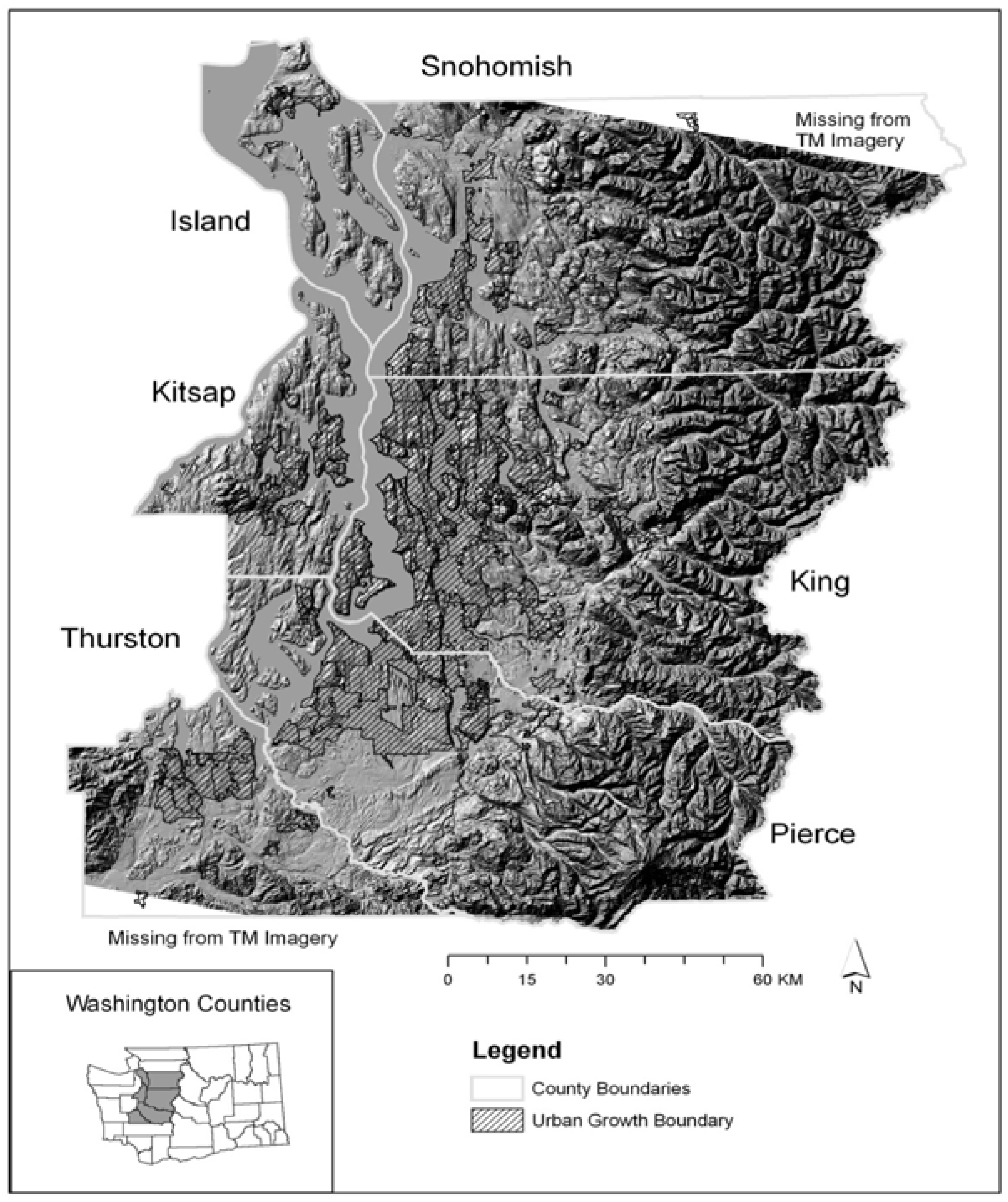
Our objective in this study was to develop a multi-date land cover database for the urbanizing Central Puget Sound region of western Washington State, USA, and to examine change in composition and configuration of land cover over a twenty year time span. Due to the high heterogeneity of urban landscapes and our desire to increase both the spatial and class resolution, traditional satellite image classification techniques were insufficient. We developed a technique that combined multiple methods, each targeted at classifying a specific land cover class and maximizing class separation. We used supervised classification, spectral unmixing, image segmentation, multi-date and multi-season imagery, and temporal landscape trajectory rules to accomplish our task. Our specific objectives were: (1) develop a multi-date land cover classification for highly heterogeneous urban environments using mixed classification methods, post-classification techniques, and landscape trajectory analysis to improve class resolution and accuracy of our classifications; (2) document amounts and changes in land cover composition and configuration from 1986-2002; and (3) assess the accuracy of our classifications.

2. Methods

2.1. Study Area

Our 20,300 km2 study area (17,800 km2 land area) includes the six counties (Island, King, Kitsap, Pierce, Snohomish, and Thurston) surrounding the Central Puget Sound of western Washington, USA, (Figure 1) and contains all or portions of the major metropolitan areas of Seattle, Tacoma, Bellevue, and Everett. This region has experienced dramatic urban growth, especially during the last 30 years [13,47] and is projected to grow by 41% (an additional 1.2 million people from 2000) by 2030 [48]. Documenting land cover change from 1986-2002 is important in understanding how the structure of the landscape has changed and is an important first step to understanding how ecological processes may have changed over this time period.
Figure 1. Six county study area in western Washington, USA showing the 2002 Urban Growth Areas, elevation, water, and county boundaries.
Remotesensing 01 01353 g001

2.2. Satellite Data Acquisition and Processing

Our study area fell within the extent of a single Landsat Thematic Mapper (TM) or Enhanced TM (ETM+) scene. We acquired a total of 10 images for five years (1986, 1991, 1995, 1999, and 2002) with leaf-on (June-July) and leaf-off images (March-April) for each year. Ideally we would have had imagery for every four years (or a constant interval), but cloud cover, atmospheric interference, and sensor problems made this impossible. Multi-season data has been successfully used in the past [49,50] to differentiate land cover classes that may be spectrally similar in one season and dissimilar in another. While the winter months of December and January are ideal for leaf off images, the low sun angle which increases shade effects and snow cover in the mountains makes these images less than practical for our analysis. We instead acquired leaf-off images from March and early April when the sun elevation angle is not as severe and the snow pack has typically receded to higher elevations, but leaf-out has not yet commenced.

2.3. Data Preparation

We applied a series of data preparation steps to all scenes prior to land cover classification. Many of the pre-classification processing steps were performed using ENVI 4.x (ITT Visualization Information Solutions). Other steps, including all classification methodologies were performed using Erdas Imagine 8.6 (Leica Geosystems). Each image was co-registered to the July 7, 1991 image to Universal Transverse Mercator projection, North American Datum 1983 with 30-m pixel resolution using nearest neighbor resampling and a root mean square error of less than 0.5 pixels for each image. We applied a series of radiometric corrections to the image data. All Landsat TM and ETM+ images were pre-processed by USGS using standard geometric and radiometric correction methods including correcting for location and terrain errors. We converted all TM images to the radiometric calibration of ETM+ using data conversion algorithms provided by the U.S. National Aeronautics and Space Administration (NASA) [51]. We converted the digital number values for each band to radiance at satellite (LS) values using gain and bias values from NASA [51]. We used dark object subtraction on each band to correct for atmospheric scattering [52]. We then calculated at-satellite reflectance, correcting for seasonal illumination differences caused by varying earth sun distance and sun elevation angles [53]. We used a 10-m Digital Elevation Model and cosine solar incidence angle to correct for topographic errors. Finally, we used spectral inter-calibration to correct any lingering spectral differences between images that were not the result of land cover change [52,54]. We identified and digitized pseudo-invariant objects with varying degrees of albedo and the average spectra of each object was recorded and regressed against the corresponding object-values from the 1999 summer image (our clearest recent image). The resulting gain and offset from the regression equation was applied to each year-band combination to inter-calibrate to the corresponding band in the 1999 image.

2.4. Classification Scheme

Our target classification scheme included 14 classes (Table 1) which were identified through the steps outlined below. The surface heterogeneity of urban areas leads to spectrally heterogeneous imagery at small spatial scales. Because the level of impervious area is an important determinant of many ecosystem processes [29,55], we attempted to separate urban areas into four classes: heavy (>80% impervious surface), medium (50–80% impervious surface), and light (20–50% impervious surface) intensity urban, and land cleared for development (bare land that became urban in subsequent dates).
Table 1. Preliminary 9-class and final 14-class land cover classification schemes.
Preliminary ClassificationFinal ClassificationCodeClass Definition
Heavy Intensity UrbanHeavy Intensity UrbanHIU> 80% Impervious Area
Medium Intensity UrbanMedium Intensity UrbanMIU50–80% Impervious Area
Light Intensity Urban Light Intensity UrbanLIU20–50% Impervious Area
Land Cleared for DevelopmentLCDLand that was vegetated in a previous time step and urban in a later time step
GrassGrassGRDeveloped Grass and Grasslands
Bare Soil Non-vegetated (mixed agriculture, urban, clearcut forest)
AgricultureAGRow Crops, Pastures
Deciduous and Mixed ForestDeciduous and Mixed ForestDMF>80% Deciduous Trees,10–80% each Decid./Conif. Trees
Coniferous ForestConiferous ForestCF>80% Coniferous Trees
Clearcut ForestClearcut ForestCCClearcut Forest
Regenerating ForestREGRe-growing Forest
Open WaterOpen WaterWATWater
Non-forested WetlandsNFWNon-forested Wetlands
ShorelineSHOTidal areas bare during low tide
Bare Rock /Ice/SnowROCK High elevation areas with no vegetation or snow cover

2.5. Image Classification Protocol

Our general approach to classification was interactive and hierarchical (Figure 2). We started with broad classes and worked within these classes to disaggregate them into more detailed classes. We used several classification techniques throughout the process to achieve a final classification for each year. Our starting point was a top-level classification in which each summer image was segmented into three categories (vegetation, non-vegetation, and water) using a combination of spectral unmixing (spectral mixture analysis) and supervised classification (Figure 2A,B). With all supervised classifications we used high-resolution digital orthophotographs to identify specific land cover types including dense urban surfaces (e.g., pavement, roofing surfaces), mixed-urban areas (e.g., residential), grasses, clear-cut, deciduous and mixed forest, conifer forest, bare soil, and agricultural lands. We then used spectral unmixing, supervised classification, or both on separate image segments (i.e., pixels identified as vegetation or non-vegetation) to disaggregate each segment into specific land cover classes.

2.6. Preliminary Nine-Class Maps

We began by segmenting our images into vegetation (deciduous forest, coniferous forest, green grass), non-vegetation (urban, mixed urban, bare soil, dry grass, and grasslands), and water using supervised classification and spectral unmixing in combination. Supervised classification was done on each summer 6-band image with the summer NDVI image added as a seventh band (Figure 2A) and spectral unmixing [38] was performed on each 6-band summer image to separate non-vegetation (soil and urban pixels), vegetation (forest and agriculture), and shade/water (Figure 2B). Spectral end members were selected based on the following criteria: (1) they must exist as unique spectra that bound the majority of the pixels in the data cloud, (2) they must exist on a general linear plane between the other end members, and (3) they are not extreme pixels. We combined the results from the spectral unmixing and the preliminary supervised classification as follows: (1) pixels with ≥75% shade end member and ≤20% vegetation end member and the supervised water class were classified as water; (2) pixels where the shade normalized vegetation end member image was >80% of the pixel were added to the supervised vegetation class and classified as vegetation; and (3) the remaining non-vegetation pixels from spectral unmixing were added to the supervised non-vegetation class and classified as non-vegetation.
Figure 2. Classification steps, landscape trajectory analysis, and ancillary GIS-derived classes used to develop the 14 land cover classes for each year of imagery.
Remotesensing 01 01353 g002
We next separated non-vegetation pixels into clearcut forest, cleared agriculture (bare soil), or urban classes. We used different techniques to identify these classes. Clearcuts are created as large homogeneous patches of non-vegetation that quickly return to vegetation. We used spatial and temporal patterns in the imagery to differentiate these areas from urban patches. We used supervised classification on bands 3-6 from our target year and those of our two endpoints (1986, 2002) from the non-vegetation image segment for each year (Figure 2C). We selected trainings sites for observed clearcuts. While the inference available for our end dates is less strong than for those dates bounded by our endpoints, the method was still applicable throughout our time series. We differentiated between urban and agriculture classes by comparing the pixel-specific variance in band 4 across all dates and adding this index to each date’s 6-band summer image (Figure 2D). We hypothesized that agricultural areas would display greater variance in the near-infrared portion of the spectrum than would urban areas because agricultural areas are cleared, planted, and harvested within a growing season and between years whereas urban areas experience a single flush of vegetation and senescence during the growing season and once impervious, remain impervious. We used supervised classification on the non-vegetation pixels in the 7-layer images using signatures for urban, mixed urban, grass, and agriculture (bare soil). We used the urban and mixed urban classes from this classification to further segment the image into urban classes. We then used spectral unmixing on these urban pixels (Figure 2E) to separate heavy urban (80–100% impervious), medium urban (50–80% impervious, and light urban (20–50% impervious).
For vegetation pixels identified in the first image segmentation (Figure 2B), we used supervised classification of the 6-band summer image plus NDVI for each year to separate forest from grass/shrub/agriculture (Figure 2F). To further differentiate forest types, we used a second supervised classification for each year using signatures for conifer and mixed forest classes on leaf-off and leaf-on images and bands 3-6 for each year (Figure 2G). Finally, we combined all classified image segments representing water, non-vegetation and vegetation classes from above into a preliminary 9-class classification for each year (Table 1).

2.7. Landscape Trajectory Analysis

Our multi-temporal dataset provided the opportunity to use temporal patterns in land cover to further differentiate confused classes and correct for classification errors in the preliminary 9-class datasets. Intuitive landscape trajectory rules were developed for plausible combinations of classes among our five years of land cover data. For example, heavy intensity urban in 1986 would not be expected to become coniferous forest in any later date. Specific rules were developed for each of the final land cover classes in Table 1. For example, Bare Soil in the preliminary classification was split into Cleared for Development (if the pixel was forested at an earlier date and became one of the developed classes at a later date), Agriculture (if bare soil or grass in prior/later dates), or Clearcut (if later a forest class and above 300 m elevation) (Figure 2H). Clearcut was constrained to those pixels forested in the previous time step and above 300 m elevation because commercial timberland primarily occurs in the higher elevations surrounding Seattle and previous experience indicated this threshold would clearly differentiate harvesting operations from site conversion. Regenerating Forest was derived from Clearcut pixels in the previous time step.
Because of yearly environmental differences (primarily wetness) between satellite images, the exact separation between urban land cover classes was variable between dates, leading to temporal sequences such as Heavy Urban-Medium Urban-Light Urban-Medium Urban-Heavy Urban. Two dates, 1991 and 1999, representing the best original imagery, were chosen as base classifications from which to determine when urban classes for the other dates were incorrect (Figure 2I). Urban classes were constrained to maintain or increase intensity over time, since urban abandonment was uncommon during this time period. If there was a disagreement between 1991 and 1999 urban classes, the 1999 class designation prevailed.

2.8. GIS Overlays

We derived several land cover classes from ancillary GIS data (Figure 2J), including: (1) Open Water (lake or pond, ditch or canal, stream or river, bay, estuary, gulf, ocean/sea, and reservoir derived from 1:24,000 scale hydrography from WA Department of Natural Resources [WADNR]); (2) Non-Forested Wetlands (marsh, wetland, swamp, bog, and cranberry bog from WADNR hydrography); (3) Shoreline (tidal, mud, sand, and gravel flats from WA Department of Ecology [WADOE] 2001 Marine Shorelines); and (4) Rock/ice/snow (glacier or permanent snowfield: WADNR hydrography). These classes were “burned-in” to the final classifications for all dates. Each of these ancillary GIS data layers have errors associated with omission, commission, and temporal mismatches with our multi-date TM data. Because of this, we made no effort to ascertain the accuracy of these classes in our final maps.

2.9. Land Cover Composition and Configuration over Time

We were interested in documenting how the landscape has changed over time. We calculated several landscape metrics of composition (area and percentage of each land cover class) and configuration for each date using the 30-m map grain [56]. Metrics can be calculated on individual land cover classes or for all classes at once. We grouped urban classes, grass and agriculture, and forest classes and calculated class metrics for each (number of patches[NP], mean patch size [MPS], edge density [ED], landscape shape index [LSI], percentage of like adjacencies [PLADJ], and aggregation index [AI]) using Fragstats 3.3 software [56]. We chose these metrics for several reasons. Metrics measuring patch dynamics (NP, MPS) are metrics describing the fragmentation of a patch type. Edge density (the length of class edge per hectare of the study area) is an indication of how much of a class exists as edge pixels. Landscape shape index, PLADJ (class-specific contagion), and AI (internal like-adjacencies) all measure slightly different aspects of class aggregation [56]. These simple metrics have been used in many other studies including studies of urban landscape pattern and change over time [23,28,57,58,59,60,61]. These metrics, and other similar metrics, have also been used by many ecological studies to document how ecosystems [62] or species respond to landscape pattern [14,63].
We also compared landscape change within and outside of a 2002 “urban growth boundary”. These areas are designated as such by town, city, or regional planning departments inside of which urban development is encouraged [64]. If these policies are having their intended effects, we would expect more development (as a percentage of the total new development) would occur within these boundaries. A more complete exploration of the changes in landscape pattern in our study region by various political boundaries is under way in a separate study.

2.10. Land Cover Reference Data and Accuracy Assessment

We developed reference datasets for each year using high resolution (0.3–1 m) large map scale (1:9,600 to 1:30,000) black and white scanned aerial photographs (1986) and true color digital orthophotographs (1991, 1995, 1999, 2002) for selected areas throughout our study area. A 90 m fishnet was developed for the study area and 10% of the polygons were randomly selected for identification and typing using aerial photography. An independent photo interpreter typed each cell to one of our final land cover classes (Table 1) only if located on a homogeneous patch of land cover. The number of reference sites for each class for each year ranged from 37 to 102 (Appendix A).
We generated standard contingency tables [65] comparing reference and classified data using the majority land cover class within the 90 m reference cell. We compared the preliminary 9-class datasets and the final 14-class datasets created from the class trajectory analysis to determine if our methods improved class accuracy. We tested for a significant difference between the Kappa accuracy of preliminary and final classifications [65]. We did not attempt to assess the accuracy of those classes derived from ancillary GIS layers. Additionally, the Land Cleared for Development class did not occur frequently enough in our aerial photographs to adequately assess, so that class was combined with Light Urban in our land cover maps prior to conducting the accuracy assessment. Since our Medium Urban and Light Urban classes contained mixed pixels and represented land cover types that are heterogeneous at spatial extents larger than our 30 m pixel scale, we evaluated the accuracy of our classifications at spatial extents larger than single 30 m pixels: we tabulated the individual number of urban pixels within the 90 m reference polygon to determine the proportion of urban class pixels within each urban class reference polygon.

3. Results and Discussion

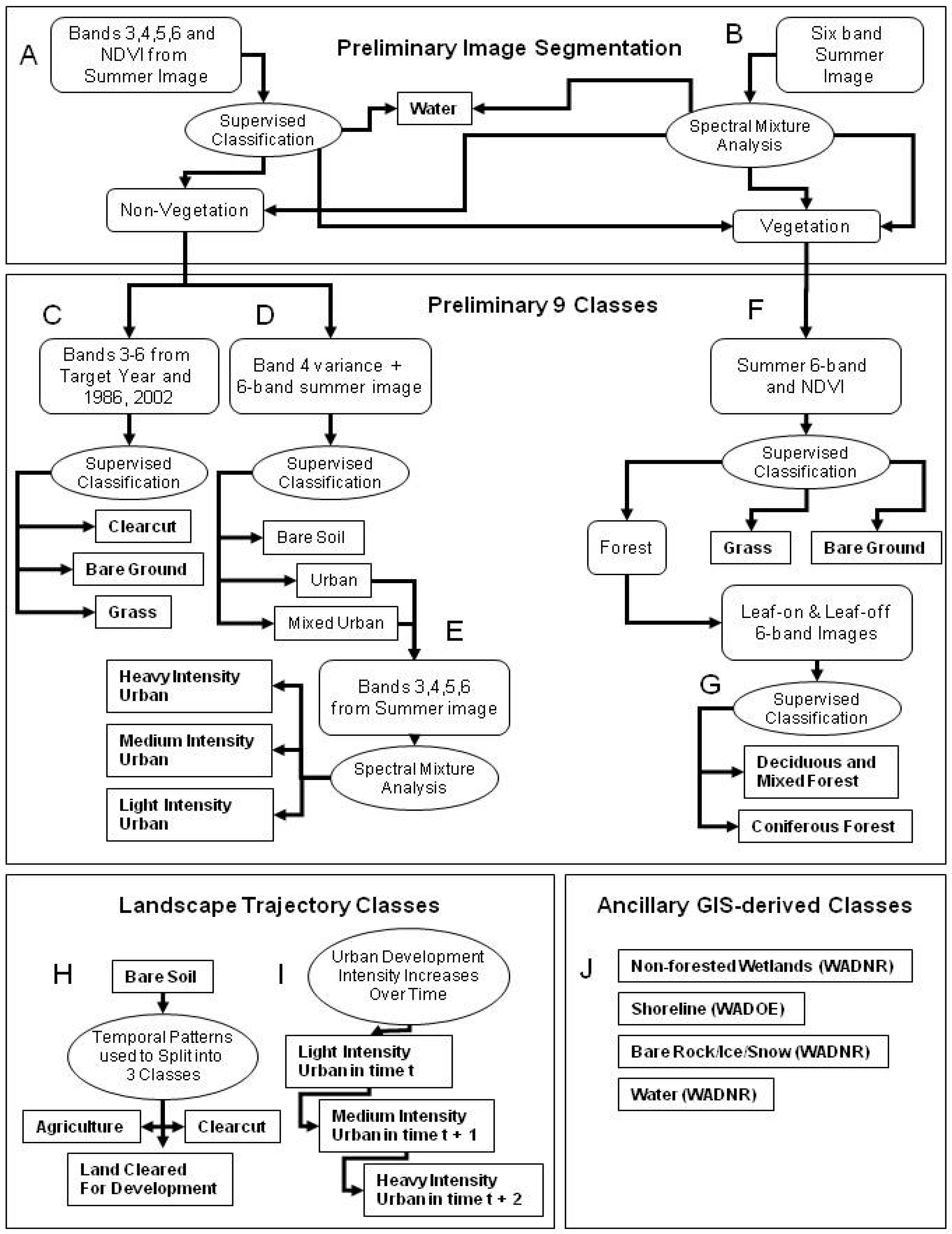
Our study combined image segmentation, supervised classification, spectral mixture analysis, time series analysis, GIS data integration, and trajectories of landscape change to derive five dates (1986, 1991, 1995, 1999, and 2002) of land cover at a relatively high spatial resolution (30 m) for a large, highly heterogeneous, and changing urban region. The use of these techniques in concert allowed us to map 14 land cover classes, including three classes of urban land cover, and compare both the composition and configuration of the landscape over time.

3.1. Land Cover Classifications and Landscape Trajectories

We developed 9-class maps for all five dates using the methods described above. These preliminary maps did not differentiate between grass, agriculture, and land cleared for development. In these preliminary maps there was considerable confusion between Deciduous and Mixed Forest (DMF) and Coniferous Forest (CF) classes and between different classes of urban with intensity (i.e., heavy, medium, light) varying between dates. In addition, areas of cloud and cloud shadow were classified as urban or as water, respectively. To address these problems, we used a series of landscape trajectory rules, each developed specifically for an observed problem. For example, if a pixel was classified as a higher intensity of urban in two or more, earlier dates, it was assumed to remain at least that intensity of urban into the future. In general the urban class confusion was between High and Medium or Medium and Low Intensity Urban classes. We illustrate the effect of this rule for transitions between 1986 and 1991 (Table 2). We addressed the confusion between DMF and CF by classifying a pixel to the majority class from across all five dates, weighted towards CF at elevations above 300 m above sea level and towards DMF at elevations below 300 m. We separated grass and bare soil into Grass (GR), Agriculture (AG), Land Cleared for Development (LCD), and Clearcut (CC) using the temporal patterns observed in the 9-class maps. Specifically, GR would remain grass over time; AG would vary between grass and bare soil over time; LCD would start out in a class with vegetation, become a class without vegetation [LCD], and then become an urban class; Clearcut would begin as forest and change to bare soil or grass.
Table 2. Change in urban land cover class area (km2) between 1986 and 1991 for the preliminary (hybrid classification approaches applied) and final (landscape trajectory post-classification rules applied) maps.
Preliminary Nine Class1986
HUIMUILUITotal
1991HUI777124969
MUI262588231
LUI462253162,7641
Final Fourteen Class
1991HUI235347
MUI 558136
LUI 4581,427
Note: 1 Class and total contained many cloud-affected pixels
While it would be useful to have a standard set of trajectory rules, it is unlikely that such rules exist given that each landscape is undergoing transitions potentially driven by many different factors [19,66]. In areas where urbanization is driving anthropogenic landscape change, assumptions can be made that land use is becoming more intensive and therefore land cover is likely increasing in impervious surfaces [40].

3.2. Land Cover Amounts and Patterns over Time

Our study region, the Central Puget Sound, is dominated by forests, with lesser amounts of water, urban, grass, and agriculture (Table 3). Over our 16 year study period, urban land cover increased from 1,632 km2 (8.0%) in 1986 to 3,661 km2 (18.0%) in 2002 in our six county study area (Table 3). The majority of new urban areas in our study were Deciduous and Mixed Forest (DMF) in 1986 with 1,291 km2 DMF lost by 2002 (from 20.8 to 14.4%) and 800 km2 lost in Grass (GR) and Agriculture (AG) classes (from 11.4 to 7.5%). While urban land cover increased steadily from 1986–2002, the loss of DMF, GR and AG was non-linear, alternating which land cover class was predominately being converted to urban land cover (Table 3). The total area in forest (DMF, CF, CC, and REGEN) decreased between 1986 (12,420 km2) and 2002 (11,045 km2) with losses in Conifer Forest replaced by Clearcut and Regenerating Forest (Table 3). Actual losses in Conifer Forest in 2002 may be masked by the larger snowpack in the 2002 TM images.
Our study found patterns similar to other recent studies. For example, Ji et al. [23] documented a steady increase in urban lands, from 8.7% in 1972 to 19.2% in 2002, with the conversion of lands primarily from non-forested lands for the 8,215 km2 surrounding and containing the Kansas City metropolitan area. In the 7,000 km2 Twin Cities Metropolitan Area, urban land increased from 23.7% to 32.8% of the total area, with losses primarily in Agriculture [27]. Other cities surrounded primarily by forest have also seen a similar loss of forests to urban lands. For example, Boentje and Blinnikov [28] observed between 14–35% of mature forest lost in the districts surrounding Moscow’s Green Belt from 1991 to 2001.
Table 3. Six county study area amount (km2) and percent (%) of study area for each land cover class and three class groupings for 1986, 1991, 1995, 1999, and 2002.
1986 1991 1995 1999 2002
km2%km2%km2%km2%km2%
HIU2521.23211.63851.94912.46393.1
MIU6443.28924.41,0955.41,1665.71,3016.4
LIU7203.51,0855.31,2486.11,4317.01,7068.4
LCD150.1520.3440.2450.2150.1
GR1,7548.61,6768.21,8709.21,5397.61,1425.6
AG5752.87913.95342.64822.43881.9
DMF4,22620.83,78118.63,80818.73,15915.52,93514.4
CF6,90633.96,02829.65,46426.85,65827.85,77428.4
CC7143.53131.52951.42641.37753.8
REGEN5742.88384.11,1385.614016.91,5617.7
NFW1080.5900.4900.4900.4900.4
OW2,55312.52,66613.12,63813.02,57612.72,62612.9
ROCK1,2776.31,8018.81,7248.52,03210.01,3836.8
SHORE430.2270.1270.1270.1270.1
Total Urban11,6328.02,35011.52,77313.63,13315.43,66118.0
GR & AG2,32911.42,46712.12,40411.82,0219.91,5307.5
Total Forest212,42061.010,96053.810,70652.610,48251.511,04554.2
Notes:
  • 1 Total Urban include four urban classes (HIU, MIU, LIU, and LCD).
  • 2 Total Forest includes forest classes (DMF, CF, CC, and REGEN).
As areas become more urban, the patterns of land cover change. We were interested in documenting these changes since landscape patterns influence regional biodiversity [19,63,
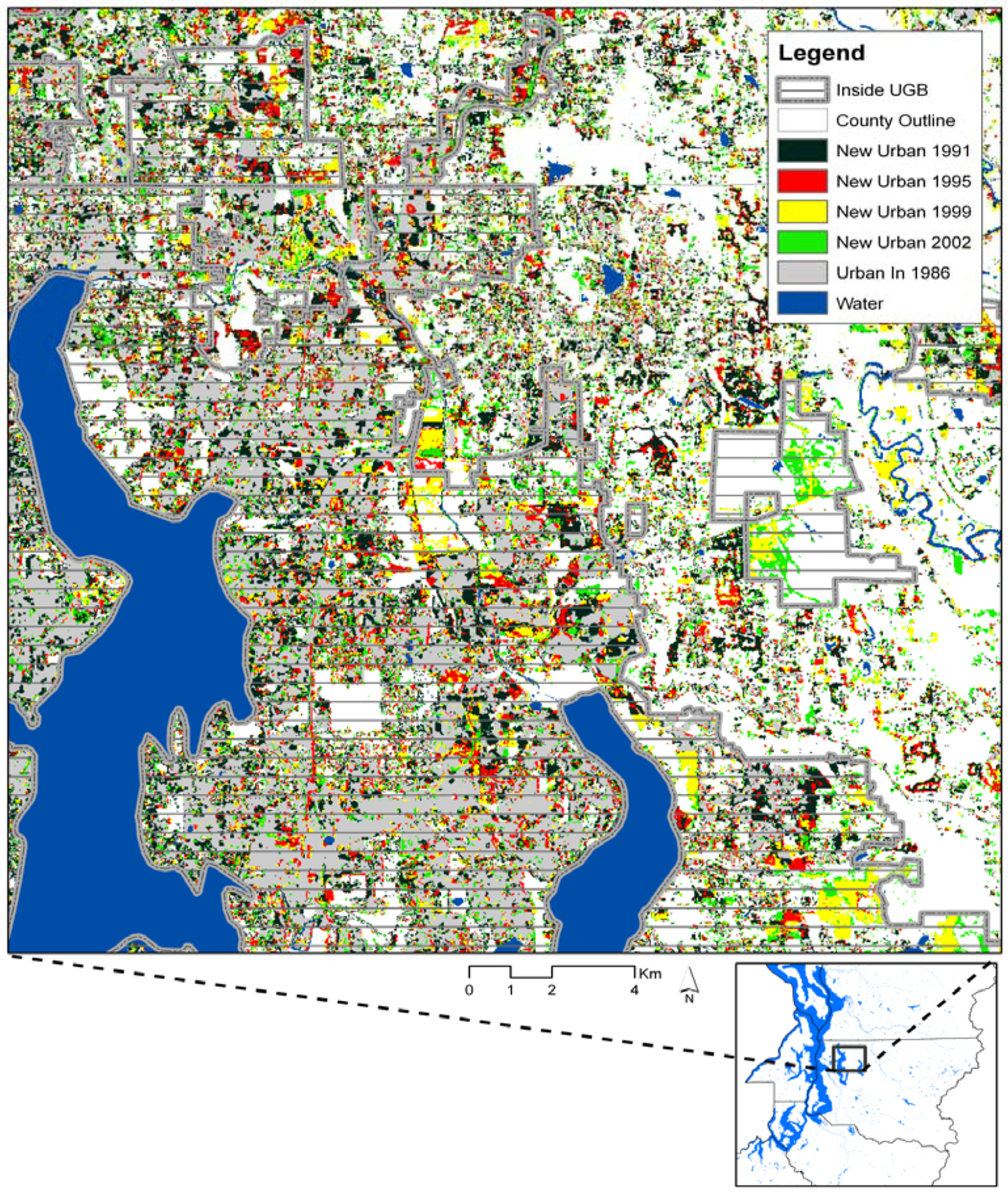
67]. Between 1986 and 2002, urban areas spread out from the existing cities of Seattle, Bellevue, Tacoma, Olympia, Everett, and Bremerton, into the lower elevations and up canyons. Urbanization seemed to increase regardless of location within or outside of Urban Growth Boundaries with Figure 3 showing a zoomed-in view northeast of downtown Seattle. Many new patches of urban are clearly visible in 1991 with subsequent areas often adjacent to these. Many large contiguous areas were developed between 1995–1999 and 1999-2002, clearly corresponding to the rapid growth of the area during this period.
The configuration of the landscape changed greatly between 1986 and 2002 (Table 4) with both the number of patches and patch density of urban peaking in 1991, but mean patch size of urban increasing across the same time period, indicating a consolidation of urban patches over time. Both GR and AG and Forest patches decreased in mean size with Forest becoming more patchy (larger NP) and more irregular in shape (larger LSI). Most other metrics for GR and AG peaked in 1995, indicating a change in the overall pattern of these classes at that time. PLADJ and AI, both measures of the dispersion of patches with lower values indicating more dispersed patches of the focal class, decreased for Urban and increased for both GR and AG and for Forest (Table 4).
The ecological implications of the change in composition (Table 3) and configuration (Table 4) of our study are many. Species associated with forests and/or grass and agriculture were likely reduced in regional abundance and diversity both from absolute loss of habitat area, but also through the fragmentation of remaining habitat patches (e.g., more patches but with a smaller mean patch size). The separate and potentially additive effects of habitat composition and configuration on species occupancy of sites have been well documented in a variety of taxa [5,68,69,70]. Companion studies have used these land cover maps in several studies. Hepinstall et al. [14] used three dates (1991, 1995, and 1999) to build and test (using 2002 land cover) a land cover change model that predicted land cover 25 years into the future. Hepinstall et al. [63,71] used the 2002 land cover to develop avian species richness models and output from land cover and urban development models to predict possible changes in avian richness by 2027.
Figure 3. Urban land cover from 1986 to 2002 showing when land transitioned to urban classes with respect to the 2002 Urban Growth Boundaries (UGB).
Remotesensing 01 01353 g003
Table 4. Basic land cover composition and configuration metrics over time (NP = number of patches, MPS = mean patch size [ha], ED = edge density [m/ha], LSI = landscape shape index, PLADJ = percentage of like adjacencies, AI = aggregation index [56].
YearNPMPSEDLSIPLADJAI
Urban1198677,6482.122.7306.477.277.3
199191,9592.632.8365.377.477.4
199583,8473.333.4348.480.280.2
199984,7473.735.0346.881.481.5
200278,3154.734.0337.483.383.3
GR & AG1986236,3401.038.9541.766.366.4
1991227,4851.146.0563.566.066.0
1995308,3320.849.7630.461.461.5
1999283,9470.743.3603.059.859.8
2002257,1510.631.1561.256.957.0
Forest2198671,84515.533.7310.191.291.2
199188,12511.144.4341.589.789.7
199589,81410.347.0367.188.688.6
199996,6919.142.8368.788.288.2
2002106,4238.237.2412.786.786.8
Notes:
  • 1 Urban includes four urban classes (HIU, MIU, LIU, and LCD).
  • 2 Forest includes four forest classes (DMF, CF, CC, REGEN).
Table 5. Land cover area (km2) and percent (%) of class over time inside (first row each year) and outside (second row each year) of the 2002 Urban Growth Boundaries (UGB).
19861991199519992002
km2%km2%km2%km2%km2%
Urban11,166.771.51,459.062.11,635.159.01,747.655.81,883.851.5
464.928.5891.437.91,138.141.01,386.044.21,777.448.5
GR & AG488.521.0409.816.6341.814.2283.714.0175.711.5
1,841.079.02,057.383.42,062.285.81,737.686.01,354.088.5
Forest21,007.88.1794.97.3689.66.4635.46.1606.35.5
11,412.691.910,165.792.710,016.893.69,847.293.910,438.694.5
Notes:
  • 1 Urban includes four urban classes (HIU, MIU, LIU, and LCD).
  • 2 Forest includes four forest classes (DMF, CF, CC, REGEN).
In Washington State, a 1990 state law mandated the delineation of Urban Growth Boundaries (UGB), inside of which urban development is encouraged [64]. We compared the area and percent of each class falling inside or outside of the 2002 UGBs and summarize our finding here for summary classes (Urban, Grass and Agriculture, and all Forest; Table 5). While land cover changed differentially within and outside of the 2002 UGB and the total area of urban steadily increased over time, we observed an increase in the percentage of urban areas outside of the UGB from 28.5% in 1986 to 48.5% in 2002. The area in Grass and Agriculture declined greatly during this same time period, with a lower percentage inside the UGB by 2002. Both the area and percent of total forest (including Clearcut and Regenerating forests) decreased over time inside the UGB. Clearly urbanization was proceeding both inside and outside of the UGB with the change coming at the expense of both GR and AG and Forest (Table 5).

3.3. Land Cover Accuracy Assessment

We compared class accuracy of major land cover classes (Urban, Grass and Agriculture, and Forest) for preliminary and final land cover maps (Table 6). Overall classification accuracies for our major classes were high, ranging from 79.5 to 89% with kappa values of between 0.687 and 0.841 (Table 6). The accuracy of Grass and Agriculture was consistently higher with our final classification often at the cost of accuracy of our final urban classes; likely because our Light Intensity Urban class represented a mixed land cover class as well as the difficulty of locating reference samples for this class. The 14-class maps had significantly higher overall accuracy (kappa) for 1986 and 1991 and significantly lower accuracy for 2002. The lower accuracy in 2002 was from a larger number of grass and agriculture reference sites being classified as urban classes (Appendix A). The application of landscape trajectories for 2002 improved user’s accuracy for some classes and producer’s accuracy for others (Table 6, Appendix A). For 2002 the use of landscape trajectory rules for urban classes may have overestimated the amount of urban land; however it is also possible that the photo interpretation underestimated the true extent of the Light Intensity Urban class.
We also generated error matrices showing the number of reference sites and user’s and producer’s accuracy for the preliminary 9-class datasets and 14-class datasets regrouped to match the 9-class datasets (Appendix A). Our final classification consistently did a better job at correctly classifying our reference sites and not over-classifying (i.e., commission errors) for all classes except Light Intensity Urban (User’s Accuracy; Appendix A). Heavy Intensity Urban, Medium Intensity Urban, Grass, Agriculture, and Clearcut user’s accuracies were substantially higher after applying the landscape trajectory rules. In addition, Clearcut and Regenerating Forest and Agriculture/Bare Soil were mapped with much higher accuracy in our final classification than in our preliminary classification (Producer’s Accuracy: Appendix A). Total accuracy ranged from 50.3% to 73.3%, was lowest for 1986 maps and was consistently higher for the final versus preliminary classifications (significantly higher for 1986, 1991, 1995, and 2002), indicating the landscape trajectory rules improved the overall accuracy of the maps (Appendix A). Previous studies have had similar success in using multi-date land cover maps and temporal rules to improve classification accuracies [12,43].
Because we did not apply any majority filters to our final land cover maps, our Light Intensity Urban pixels were often interspersed with Grass and Forest classes, making comparisons with the 90 m reference dataset difficult. In addition to the traditional accuracy assessment presented above, we tallied the number of pixels in each reference cell that were classified as Heavy, Medium, or Light Intensity Urban for our 2002 map. Using this methodology, we observed a much higher agreement between our classification and the reference data set (Table 7). For Light Intensity Urban, over 70% of our reference sites had a least one of nine pixels classified as Light Intensity Urban, our most heterogeneous urban class. Medium and Heavy Intensity Urban had a higher proportion of reference sites with clear majorities (74% and 90%, respectively). Previous attempts at pixel-based classification have also found high error rates (especially errors of commission) when attempting to classify areas of low density urban development [30].
Table 6. Class accuracy assessment (user’s and producer’s, total and Kappa-adjusted accuracy, and significance difference between two classifications at alpha 0.05) for three land cover class groupings for the preliminary and final land cover maps. For individual class accuracies see Appendix A.
ClassifiedReference DataReference Data
DataPreliminary (9 Class)Final (14 Class)
1986UrbanGrass & AgForestUser'sUrbanGrass & AgForestUser's
Urban57897884.649537492.4
Grass & Ag1113195366.01514363170.6
Forest9911196682.11094897686.1
Producer's73.460.594.1 65.683.796.5
Total 79.6 83.4
Kappa 0.678 0.741*
1991UrbanGrass & AgForestUser'sUrbanGrass & AgForestUser's
Urban830441293.7812301295.1
Grass & Ag441488353.8441787260.5
Forest632360287.556760190.5
Producer's88.668.886.4 89.082.887.7
Total 85.5 87.8
Kappa 0.757 0.800*
1995UrbanGrass & AgForestUser'sUrbanGrass & AgForestUser's
Urban67376888.968578888.8
Grass & Ag364574684.8204272590.5
Forest483871289.2465073088.4
Producer's88.980.093.0 91.276.995.7
Total 88.0 89.0
Kappa 0.818 0.833
1999UrbanGrass & AgForestUser'sUrbanGrass & AgForestUser's
Urban40263286.142694681.0
Grass & Ag20288891.122261095.0
Forest172546391.7133645590.3
Producer's91.676.697.9 96.663.596.6
Total 89.5 87.3
Kappa 0.841 0.806*
2002UrbanGrass & AgForestUser'sUrbanGrass & AgForestUser's
Urban808901688.48712293876.5
Grass & Ag305538982.313831995.0
Forest357090589.6167592891.1
Producer's92.677.689.6 98.155.794.2
Total 87.3 85.2
Kappa 0.807 0.773*1
  • * Significantly different Kappa values between 10- and 14-class maps.
  • *1 Fourteen-class map accuracy significantly lower than 10 class map.
Table 7. Accuracy of urban classes (Heavy, Medium, Light) using a cutoff of number of pixels from 1 to a ≥ 5 (a clear majority) of 9 pixels in each 90 m × 90 m reference assessment polygon for the final 2002 land cover map.
HeavyMediumLight
Cutoff(N = 279)(N = 339)(N = 288)
195.392.670.5
294.688.561.8
394.386.456.6
491.880.250.0
≥ 590.373.540.6

3.4. Limitations of Approach and Future Directions

Our hybrid approach to classifying medium resolution multi-spectral satellite imagery in heterogeneous urban environments proved successful in that we were able to map three intensities of urban land and differentiate between bare soil cleared for development, agriculture, or forest harvesting with high levels of accuracy. However, there are limitations and assumptions inherent in our approach. For example, when conducting spectral unmixing, some of the literature regarding end member selection suggests using the extreme pixels that bound all other pixels in image feature space, but this requires that these pixels represent pure pixels and not statistical outliers which would skew results [37]. Locating spectral end members for urban surfaces, however, presents a unique problem in that there is a tremendous degree of spectral variance among urban reflectance. Previous research has shown that pure impervious surfaces tend to lie along an axis of low to high albedo spectrum. As a result, pure urban pixels often exist without actually being end members because they fall somewhere between low and high albedo (non-vegetation) end members [38,72,73]. If an urban pixel does contain bare soil, this component will most likely be modeled as shade and impervious surface during the unmixing. Using a low albedo end member as an impervious proxy will most likely model this shade component as impervious surface, when in reality it cannot be determined whether the shade is caused by a building, tree or is in fact part of the impervious surface spectra [74].
Bare soil, similarly, did not seem to exist as a truly distinct urban end member in spectral space, but rather exists along the vector containing urban at one end and shade/water at the other. This vector extended from high albedo bare soil/urban surface through low albedo bare soil/urban surface and finally to water. The pixels along this plane (except for water pixels at the end of the plane) are some combination of urban surface, bare soil and shade. Because we used a supervised classification that separated 100% bare soil from urban pixels, we assumed that most bare soil pixels in the image were already classified and removed from the analysis in a previous step. Furthermore, because the shade fraction image was used to derive impervious estimates, urban pixels along this plane would be estimated at close to 100 percent impervious. Pixels that contain both impervious surface and bare soil, however, were likely difficult to detect.
Another possible limitation of our results concerns our reference data. The reference data sets were interpreted without the benefit of stereo pairs and in the case of 1986, were in black and white. Because the reference data were derived from aerial photographs with differing spectral and spatial resolutions, some classes may have been interpreted differently across time. For example, differentiating between deciduous, mixed, and coniferous forest was more problematic with the older imagery. In addition, precisely matching the three classes of urban across time was problematic for the photo interpreter.
Several of our classes were added to our land cover map through the use of ancillary GIS data layers. Each of these classes, therefore, has their own temporal relevance and location errors. For this reason, we used only GIS data for classes that were unlikely to change significantly over our study time period. Roads were not used to aid in classifying urban classes because there was likely significant change in roads between 1986 and 2002 and the only available spatial dataset depicted roads as of 2001 for our study area.
Previous studies have measured the patterns of urban development change over time (e.g., [75]). We used both multi-season imagery for each date and rules of landscape trajectory to differentiate those bare soil pixels that represented agriculture, clearcuts, or land cleared for development. A recent study exploring the increase in impervious surface over time used temporal rules to improve classification accuracy [40]. Another recent study used classification techniques (Principal Components Analysis) on multiple dates of imagery to improve the classification of landscape change [76]. Future work needs to determine how applying post-classification rules of change may influence pattern measurements and introduce errors of a different type into classified maps [77,78].
We used dates of imagery that were three to five years apart because of image availability. For this region, where urbanization was an important process driving landscape change, this time interval was large enough for measurable change to have occurred. Shorter time periods may have been too short to observe change and longer time intervals may have masked changes especially in Medium and Light Intensity Urban classes where vegetation re-growth over time may mask the amount of impervious surfaces present. In addition, the number of time steps increases the ability to use landscape trajectories. Our inferences for the first and last dates were limited to including data only after or only before, respectively, the target date. Longer time spans would allow further separation of land cover types with high temporal variability (e.g., agriculture, urbanization, forest harvesting and re-growth).
Measuring the accuracy of land cover change presented several challenges. For one, it is difficult to select sites of land cover change before completing a classification. The simplest estimate of accuracy of land cover change is to multiply the individual class accuracies between two dates [27]. It is also possible to report the individual class accuracies of only those areas that changed or to compare aggregate measures of change versus no change. Because we had an insufficient number of reference sites available for the same location between sequential land cover maps, we were unable to directly measure the accuracy of land cover change over time.

4. Conclusions

Urban land cover in the Central Puget Sound increased dramatically between 1986 and 2002, often at the expense of forestlands. In addition, grass and agricultural areas have declined in extent. Urban patches also grew in size and became less dispersed as individual patches expanded and coalesced into larger patches. Patches of forests, grass, and agriculture all became smaller and more dispersed. Urban development has increased disproportionally in areas where development regulations were expected to limit or even reduce development. Urban land cover outside of the Urban Growth Boundaries grew from 2.6% of our land area in 1986 to 10.0% in 2002, whereas it grew from 6.7% to 10.6% of the area inside of the Urban Growth boundaries between 1986 and 2002, respectively. A more in-depth analysis of the trends in land cover change with respect to urban growth management is currently underway.
Our hybrid methods and landscape trajectory rules improved our accuracy in separating mixed classes. Segmenting vegetation and impervious surfaces increased our ability to extract impervious areas within the mixed urban classes, as observed in previous studies (e.g., [79]). Multi-season imagery assisted in the differentiation of forest types and agriculture. Multi-date imagery allowed for the development of landscape trajectory rules, which allowed for the separation of bare soil into clearcut forest, agriculture, and cleared for new development and corrected for mis-classifications in different intensities of urban classes across multiple dates.
The observed changes in our study area have profound economic and ecological implications. The ability to map these changes is the first step in many ecological analyses, especially those involving mapping wildlife habitat. Several studies have already used these maps to build models of land cover change [14], avian diversity [63,71,80], and scenario planning [81]. Access to a temporal sequence of land cover maps for large regions is important for measuring change, calculating benchmarks of sustainable development [28], and many other applications. Land cover data such as ours also can be used to calculate other “sprawl indices” (e.g., [23]) and analyze more complex landscape patterns and change [23,82,83].

Acknowledgements

We thank Krista Merry, Glenn Martin, Robin Weeks, Rebecca Coburn, Yan Jiang, Danielle Spirandelli, Lucy Hutra, and the Urban Ecology Research Lab staff and students for critical input. This research was supported by the National Science Foundation (DEB-9875041, BCS 0120024, IGERT-0114351).

Appendix A. Land cover class accuracy (user’s, producer’s, total, and kappa adjusted) and number of accuracy assessment sites (N) for preliminary (9 class), final (14 class), and the difference (accuracy for 14 class minus 10 class) for user’s and producer’s accuracy.

1986
PreliminaryFinalDifferencePreliminaryFinalDifference
User'sNUser’sN(14–10)Producer'sNProducer'sN(14–10)
HU3417257832278766473–13
MU7634689281136838666379–2
LU5116547172–426327273041
GR15479272861253137591336
DMF586826162736957467564–1
CF5744855455–27733276330–1
CC/REG5246865134191243712017
AG/Bare SoilNA483332NA13907038969
WATER92509051–210046100460
Total50.3 62.0
Kappa0.420 0.550*
1991
PreliminaryFinalDifferencePreliminaryFinalDifference
User'sNUser’sN(14–10)Producer'sNProducer'sN(14–10)
HU7135291262209426790265–4
MU63368654082673457933512
LU6716667184–134328393175
GR1324732151184967706920
DMF703277230128726384256-3
CF8226083258192231922340
CC/REG771019410517382035119512
AG/Bare Soil792871143–7151487014655
WATER10010210010201001021001020
Total65.0 73.3
Kappa0.601 0.695*
1995
PreliminaryFinalDifferencePreliminaryFinalDifference
User'sNUser’sN(14–10)Producer'sNProducer'sN(14–10)
HU622326422925625855266–1
MU6733673332678288842896
LU5418944210–104821147197–2
GR3950461271217426764255–9
DMF6844474406785354863501
CF553026225879417892175–2
CC/REG7752801623172345423837
AG/Bare Soil7836882021093045930150
WATER100599760–3986098590
Total58.6 69.1
Kappa0.529 0.649*
1999
PreliminaryFinalDifferencePreliminaryFinalDifference
User'sNUser’sN(14-10)Producer'sNProducer'sN(14-10)
HU751588014248913485133-4
MU452655321488214679145-3
LU614454170-7171605616340
GR6730582163168125057236-24
DMF842618722949124084239-7
CF8319377206-695169951671
CC/REG71515569-16566458652
AG/Bare Soil82118375171265212045
WATER984010037310039100370
Total70.0 72.7
Kappa0.652 0.687
2002
PreliminaryFinalDifferencePreliminaryFinalDifference
User'sNUser’sN(14–10)Producer'sNProducer'sN(14–10)
HU7432672348–288275932725
MU5745452469–67833373334–6
LU6713545321–22342685128217
GR4764077221317838547365–31
DMF6555480414157647272456–3
CF7142875394385359873382
CC/REG773063212–13112017019159
AG/Bare Soil6733891822273305032443
WATER6476965432925398536
Total61.7 68.1
Kappa0.557 0.636*
* Significantly different Kappa values between 10- and 14-class maps.

References and Notes

  1. Houghton, R.A. The worldwide extent of land-use change. BioScience 1994, 44, 305–313. [Google Scholar] [CrossRef]
  2. Foley, J.A.; DeFries, R.; Asner, G.P.; Barford, C.; Bonan, G.; Carpenter, S.R.; Chapin, F.S.; Coe, M.T.; Daily, G.C.; Gibbs, H.K.; Helkowski, J.H.; Holloway, T.; Howard, E.A.; Kucharik, C.J.; Monfreda, C.; Patz, J.A.; Prentice, I.C.; Ramankutty, N.; Snyder, P.K. Global Consequences of Land Use. Science 2005, 309, 570–574. [Google Scholar] [CrossRef] [PubMed]
  3. Sala, O.E.; Chapin, F.S.I.; Armesto, J.J.; Berlow, E.; Bloomfield, J.; Dirzo, R.; Huber-Sanwald, E.; Huenneke, L.F.; Jackson, R.B.; Kinzig, A.; Leemans, R.; Lodge, D.M.; Mooney, H.A.; Oesterheld, M.; Poff, N.L.; Sykes, M.T.; Walker, B.H.; Walker, M.; Wall, D.H. Global biodiversity scenarios for the year 2100. Science 2000, 287, 1770–1774. [Google Scholar] [CrossRef] [PubMed]
  4. Marzluff, J.M. Island biogeography for an urbanizing world: how extinction and colonization may determine biological diversity in human-dominated landscapes. Urban Ecosys. 2005, 8, 157–177. [Google Scholar] [CrossRef]
  5. Cushman, S.A.; McGarigal, K. Landscape-level patterns of avian diversity in the oregon coast range. Ecol. Monogr. 2003, 73, 259–281. [Google Scholar] [CrossRef]
  6. Meyer, W.B.; Turner, B.L., II. Human population growth and global land-use/cover change. Annu. Rev. Ecol. Syst. 1992, 23, 39–61. [Google Scholar] [CrossRef]
  7. Grimm, N.B.; Grove, J.M.; Pickett, S.T.A.; Redman, C.L. Integrated approaches to long-term studies of urban ecological systems. BioScience 2000, 50, 571–584. [Google Scholar] [CrossRef]
  8. Alberti, M.; Marzluff, J.M.; Shulenberger, E.; Bradley, G.; Ryan, C.; ZumBrunnen, C. Integrating humans into ecology: opportunities and challenges for studying urban ecosystems. Bioscience 2003, 53, 1169–1179. [Google Scholar] [CrossRef]
  9. Lawrence, W.T.; Imhoff, M.L.; Kerle, N.; Stutzer, D. Quantifying urban land use and impact on soils in Egypt using diurnal satellite imagery of the Earth surface. Int. J. Remote Sens. 2002, 23, 3921–3937. [Google Scholar] [CrossRef]
  10. Imhoff, M.L.; Bounoua, L.; DeFries, R.; Lawrence, W.T.; Stutzer, D.; Tucker, C.J.; Rickets, T. The consequences of urban land transformation on net primary productivity in the United States. Remote Sens. Environ. 2004, 89, 434–443. [Google Scholar] [CrossRef]
  11. Yang, X.; Lo, C.P. Using a time series of satellite imagery to detect land use and land cover changes in the Atlanta, GA metropolitan area. Int. J. Remote Sens. 2002, 23, 1775–1798. [Google Scholar] [CrossRef]
  12. Powell, S.L.; Cohen, W.B.; Yang, Z.; Pierce, J.D.; Alberti, M. Quantification of impervious surface in the Snohomish Water Resources Inventory Area of Western Washington from 1972–2006. Remote Sens. Environ. 2008, 112, 1895–1908. [Google Scholar] [CrossRef]
  13. Robinson, L.; Newell, J.P.; Marzluff, J.M. Twenty-five years of sprawl in the Seattle region: growth managment responses and implications for conservation. Landscape Urban Plan. 2005, 71, 51–72. [Google Scholar] [CrossRef]
  14. Hepinstall, J.A.; Alberti, M.; Marzluff, J.M. Predicting land cover change and avian community responses in rapidly urbanizing environments. Landscape Ecol. 2008, 28, 1257–1276. [Google Scholar] [CrossRef]
  15. Hobbs, R.; Wu, J. Perspectives and prospects of landscape ecology. In Key Topics in Landscape Ecology; Wu, J., Hobbs, R., Eds.; Cambridge University Press: Cambridge, UK, 2007; pp. 3–10. [Google Scholar]
  16. Ji, W.; Ma, J.; Twibell, R.W.; Underhill, K. Characterizing urban sprawl using multi-stage remote sensing images and landscape metrics. Comput. Environ. Urban Syst. 2006, 30, 861–879. [Google Scholar] [CrossRef]
  17. Mortberg, U.M.; Balfors, B.; Knol, W.C. Landscape ecological assessment: a tool for integrating biodiversity issues in strategic environmental assessment and planning. J. Environ. Manag. 2007, 82, 457–470. [Google Scholar] [CrossRef] [PubMed]
  18. Hansen, A.; Neilson, R.; Dale, V.; Flather, C.; Iverson, L.; Currie, D.; Shafer, S.; Cook, R.; Bartlein, P. Global change in forests: responses of species, communities, and biomes. Bioscience 2001, 51, 765–779. [Google Scholar] [CrossRef]
  19. Pearson, S.M.; Turner, M.G.; Drake, J.B. Landscape change and habitat availability in the Southern Appalachian Highlands and Olympic Peninsula. Ecol. Appl. 1999, 9, 1288–1304. [Google Scholar] [CrossRef]
  20. Wolter, P.T.; White, M.A. Recent forest cover type transitions and landscape structural changes in northeast Minnesota, USA. Landscape Ecol. 2002, 17, 133–155. [Google Scholar] [CrossRef]
  21. Chen, S.; Zeng, S.; Xie, C. Remote sensing and GIS for urban growth analysis in China. Photogramm. Eng. Remote Sensing 2000, 66, 593–598. [Google Scholar]
  22. Ji, C.Y.; Lin, P.; Li, X.; Liu, Q.; Wang, S. Monitoring urban expansion with remote sensing in China. Int. J. Remote Sens. 2001, 22, 1441–1455. [Google Scholar] [CrossRef]
  23. Ji, W.; Ma, J.; Twibell, R.W.; Underhill, K. Characterizing urban sprawl using multi-stage remote sensing images and landscape metrics. Comput. Environ. Urban Syst. 2006, 30, 861–879. [Google Scholar] [CrossRef]
  24. Epstein, J.; Payne, K.; Kramer, E. Techniques for mapping suburban sprawl. Photogramm. Eng. Remote Sensing 2002, 68, 913–918. [Google Scholar]
  25. Lo, C.P.; Yang, X. Drivers of lan-use/land-cover changes and dynamics modeling for the Atlanta, Georgia Metropolitan Area. Photogramm. Eng. Remote Sensing 2002, 68, 1073–1082. [Google Scholar]
  26. Yang, L.; Xian, G.; Klaver, J.M.; Deal, B. Urban land-cover change detection through sub-pixel imperviousness mapping using remotely sensed data. Photogramm. Eng. Remote Sensing 2003, 69, 1003–1010. [Google Scholar] [CrossRef]
  27. Yuan, F.; Sawaya, K.E.; Loeffelholz, B.C.; Bauer, M.E. Land cover classification and change analysis of the Twin Cities (Minnesota) Metropolitan Area by multitemporal Landsat remote sensing. Remote Sens.Environ. 2005, 98, 317–328. [Google Scholar] [CrossRef]
  28. Boentje, J.P.; Blinnikov, M.S. Post-Soviet forest fragmentation and loss in the Green Belt around Moscow, Russia (1991-2001): a remote sensing perspective. Landscape Urban Plan. 2007, 82, 208–221. [Google Scholar] [CrossRef]
  29. Lu, D.; Weng, Q. Use of impervious surface in urban land-use classification. Remote Sens. Environ. 2006, 102, 146–160. [Google Scholar] [CrossRef]
  30. Guindon, B.; Zhang, Y.; Dillabaugh, C. Landsat urban mapping based on a combined spectral-spatial methodology. Remote Sens. Environ. 2004, 92, 218. [Google Scholar] [CrossRef]
  31. Cadenasso, M.L.; Pickett, S.T.A.; Schwarz, K. Spatial heterogeneity in urban ecosystems: reconceptualizing land cover and a framework for classification. Photogramm. Eng. Remote Sensing 2007, 71, 169–177. [Google Scholar] [CrossRef]
  32. Rashed, T.; Weeks, J.R.; Roberts, D.; Rogan, J.; Powell, R. Measuring the physical composition of urban morphology using multiple endmember spectral mixture models. Photogramm. Eng. Remote Sensing 2003, 69, 1011–1020. [Google Scholar] [CrossRef]
  33. Ridd, M.K. Exploring a V-I-S (vegetation-impervious surface-soil) model for urban ecosystems analysis through remote sensing: comparative anatomy for cities. Int. J. Remote Sens. 1995, 16, 2165–2185. [Google Scholar] [CrossRef]
  34. Lu, D.; Moran, E.; Batistella, M. Linear mixture model applied to Amazonian vegetation classification. Remote Sens. Environ. 2003, 87, 456–469. [Google Scholar] [CrossRef] [Green Version]
  35. Lu, D.; Batistella, M.; Moran, E.; Mausel, P. Application of spectral mixture analysis to Amazonian land-use and land-cover classification. Int. J. Remote Sens. 2004, 25, 5345–5358. [Google Scholar] [CrossRef]
  36. Adams, J.B.; Sabol, D.E.; Kapos, V.; Almeida, F.R.; Roberts, D.A.; Smith, M.O.; Gillespie, A.R. Classification of multispectral images based on fractions of endmembers: application to land-cover change in the Brazilian Amazon. Remote Sens. Environ. 1995, 52, 137–154. [Google Scholar] [CrossRef]
  37. Mustard, J.F.; Sunshine, J.M. Spectral analysis for earth science: investigations using remote sensing data. In Remote Sensing for the Earth Sciences: Manual of Remote Sensing; Rencz, A.N., Ed.; John Wiley & Sons Inc.: New York, NY, USA, 1999; Volume 3, pp. 251–307. [Google Scholar]
  38. Small, C. Multitemporal analysis of urban reflectance. Remote Sens. Environ. 2002, 81, 427–442. [Google Scholar] [CrossRef]
  39. Alberti, M.; Weeks, R.; Coe, S. Urban land-cover change analysis in central Puget Sound: 1991–1999. Photogramm. Eng. Remote Sensing 2004, 70, 1043–1052. [Google Scholar] [CrossRef]
  40. Powell, R.L.; Roberts, D.A.; Dennison, P.E.; Hess, L.L. Sub-pixel mapping of urban land cover using multiple endmember spectral mixture analysis: Manaus, Brazil. Remote Sens. Environ. 2007, 106, 253–267. [Google Scholar] [CrossRef]
  41. Rashed, T. Remote sensing of within-class change in urban neighborhood structures. Comput. Environ. Urban Syst. 2008, 32, 343–354. [Google Scholar] [CrossRef]
  42. Guindon, B.; Edmonds, C.M. Large-area land-cover mapping through scene-based classification compositing. Photogramm. Eng. Remote Sensing 2002, 68, 589–596. [Google Scholar]
  43. Liu, H.; Zhou, Q. Accuracy analysis of remote sensing change detection by rule-based rationality evaluation with post-classification comparison. Int. J. Remote Sens. 2004, 25, 1037–1050. [Google Scholar] [CrossRef]
  44. Foody, G.M.; Boyd, D.S. Detection of partial land cover change associated with the migration of inter-class transitional zones. Int. J. Remote Sens. 1999, 20, 2723–2740. [Google Scholar] [CrossRef]
  45. Mas, J.F. Monitoring land-cover changes: a comparison of change detection techniques. Int. J. Remote Sens. 1999, 20, 139–152. [Google Scholar] [CrossRef]
  46. Lu, D.; Mausel, P.; Brondízio, E.; Moran, E. Change detection techniques. Int. J. Remote Sens. 2004, 25, 2365–2407. [Google Scholar] [CrossRef]
  47. Hansen, A.J.; Knight, R.L.; Marzluff, J.M.; Powell, S.; Brown, K.; Gude, P.H.; Jones, K.B. Effects of exurban development on biodiversity: patterns, mechanisms, and research needs. Ecol. Appl. 2005, 15, 1893–1905. [Google Scholar] [CrossRef]
  48. Anonymous 2007 County Projections by Single Year after 2010: Medium Projections. Available online: http://www.ofm.wa.gov/pop/gma/projections07.asp (accessed on 16 December 2009).
  49. Lunetta, R.S.; Balogh, M.E. Application of multi-date landsat 5 TIM Imagery for wetland identification. Photogramm. Eng. Remote Sensing 1999, 65, 1303–1310. [Google Scholar]
  50. Oetter, D.R.; Cohen, W.B.; Berterretche, M.; Maiersperger, T.K.; Kennedy, R.E. Land cover mapping in an agricultural setting using multiseasonal Thematic Mapper data. Remote Sens. Environ. 2001, 76, 139–155. [Google Scholar] [CrossRef]
  51. NASA Landsat 7: Science Data Users Handbook. Available online: http://landsathandbook.gsfc.nasa.gov/handbook/handbook_toc.html (accessed on 3 June 2007).
  52. Lillesand, T.; Kiefer, R. Remote Sensing and Image Interpretation; John Wiley & Sons: New York, NY, USA, 2000; p. 724. [Google Scholar]
  53. Chander, G.; Markhan, B.L.; Helder, D.L. Summary of current radeiometric calibration coefficients for Landsat MSS, TM, ETM+, and EO-1 ALI sensors. Remote Sens. Environ. 2009, 113, 893–903. [Google Scholar] [CrossRef]
  54. Cohen, W.B.; Maiersperger, T.K.; Yang, Z.; Gower, S.T.; Turner, D.P.; Ritts, W.D.; Berterretche, M.; Running, S.W. Comparisons of land cover and LAI estimates derived from ETM+ and MODIS for four sites in North America: a quality assessment of 2000/2001 provisional MODIS products. Remote Sens. Environ. 2003, 88, 233–255. [Google Scholar] [CrossRef]
  55. Tang, Z.; Engel, B.A.; Pijanowski, B.C.; Lim, K.J. Forecasting land use change and its environmental impact at a watershed scale. J. Environ. Manag. 2005, 76, 35–45. [Google Scholar] [CrossRef] [PubMed]
  56. McGarigal, K.; Cushman, S.A.; Neel, M.C.; Ene, E. FRAGSTATS: Spatial Pattern Analysis Program for Categorical Maps, version 2002; University of Massachusetts: Amherst, MA, USA.
  57. Cifaldi, R.L.; Allan, J.D.; Duh, J.D.; Brown, D.G. Spatial patterns in land cover of exurbanizing watersheds in southeastern Michigan. Landscape Urban Plan. 2004, 66, 107–123. [Google Scholar] [CrossRef]
  58. van Eetvelde, V.; Antrop, M. Indicators for assessing changing landscape character of cultural landscapes in Flanders (Belgium). Land Use Policy 2009, 26, 901–910. [Google Scholar] [CrossRef]
  59. Compas, E. Measuring exurban change in the American West: a case study in Gallatin County, Montana, 1973-2004. Landscape Urban Plan. 2007, 82, 56–65. [Google Scholar] [CrossRef]
  60. Huang, S.-L.; Wang, S.-H.; Budd, W.W. Sprawl in Taipei's peri-urban zone: responses to spatial planning and implications for adapting global environmental change. Landscape Urban Plan. 2009, 90, 20–32. [Google Scholar] [CrossRef]
  61. Rashed, T. Remote sensing of within-class change in urban neighborhood structures. Comput. Environ. Urban Syst. 2008, 32, 343–354. [Google Scholar] [CrossRef]
  62. Alberti, M.; Booth, D.; Hill, K.; Coburn, B.; Avolio, C.; Coe, S.; Spirandelli, D. The impact of urban patterns on aquatic ecosystems: an empirical analysis in Puget lowland sub-basins. Landscape Urban Plan. 2007, 80, 345–361. [Google Scholar] [CrossRef]
  63. Hepinstall, J.A.; Marzluff, J.M.; Alberti, M. Modeling Bird Responses to Predicted Changes in Land Cover in an Urbanizing Region. In Models for Planning Wildlife Conservation in Large Landscapes; Academic Press: San Diego, CA, USA, 2009; pp. 625–659. [Google Scholar]
  64. Anonymous Urban Growth Areas. http://www.commerce.wa.gov/site/402/default.aspx (accessed on 16 December 2009).
  65. Congalton, R.G.; Green, K. Assessing the Accuracy of Remotely Sensed Data: Principles and Practices; Lewis Publishers: Boca Raton, FL, USA, 1999; p. 137. [Google Scholar]
  66. Wear, D.N.; Bolstad, P. Land-use changes in southern Appalachian landscapes: spatial analysis and forecast evaluation. Ecosystems 1998, 1, 575–594. [Google Scholar] [CrossRef]
  67. Schumaker, N.H.; Ernst, T.; White, D.; Baker, J.; Haggerty, P. Projecting wildlife responses to alternative future landscapes in Oregon’s Willamette Basin. Ecol. Appl. 2004, 14, 381–400. [Google Scholar] [CrossRef]
  68. Villard, M.-A.; Trzcinski, M.K.; Merriam, H.G. Fragmentation effects on forest birds: relative influence of woodland cover and configuration on landscape occupancy. Conserv. Biol. 1999, 13, 774–783. [Google Scholar] [CrossRef]
  69. Vieira, M.V.; Olifiers, N.; Delciellos, A.C.; Antunes, V.Z.; Bernardo, L.R.; Grelle, C.E.V.; Cerqueira, R. Land use vs. fragment size and isolation as determinants of small mammal composition and richness in Atlantic Forest remnants. Biol. Conserv. 2009, 142, 1191–1200. [Google Scholar] [CrossRef]
  70. Betts, M.G.; Forbes, F.G.; Diamond, A.W. Thresholds in Songbird Occurrence in Relation to Landscape Structure. Conserv. Biol. 2007, 21, 1046–1058. [Google Scholar] [CrossRef] [PubMed]
  71. Hepinstall, J.A.; Marzluff, J.M.; Alberti, M. Predicting avian community responses to increasing urbanization. Stud. Avian Biol. in press.
  72. Wu, C. Normalized spectral mixture analysis for monitoring urban composition using ETM+ imagery. Remote Sens. Environ. 2004, 93, 480–492. [Google Scholar] [CrossRef]
  73. Wu, C.; Murray, A.T. Estimating impervious surface distribution by spectral mixture analysis. Remote Sens. Environ. 2003, 84, 493–505. [Google Scholar] [CrossRef]
  74. Dare, P.M. Shadow analysis in high-resolution satellite imagery of urban areas. Photogramm. Eng. Remote Sens. 2005, 71, 169–177. [Google Scholar] [CrossRef]
  75. Seto, K.C.; Fragkias, M. Quantifying spatiotemporal patterns of urban land-use change in four cities of China with time series landscape metrics. Landscape Ecol. 2005, 20, 871–888. [Google Scholar] [CrossRef]
  76. Deng, J.S.; Wang, K.; Hong, Y.; Qi, J.G. Spatio-temporal dynamics and evolution of land use change and landscape pattern in response to rapid urbanization. Landscape Urban Plan. 2009, 92, 187–198. [Google Scholar] [CrossRef]
  77. Shao, G.; Wu, J. On the accuracy of landscape pattern analsysis using remote sensing data. Landscape Ecol. 2008, 23, 505–511. [Google Scholar] [CrossRef]
  78. Linke, J.; McDermid, G.J.; Pape, A.D.; McLane, A.J.; Laskin, D.N.; Hall-Beyer, M.; Franklin, S.E. The influence of patch-delineation mismatches on multi-temporal landscape pattern analysis. Landscape Ecol. in press. [CrossRef]
  79. Bauer, M.E.; Heinert, N.J.; Doyle, J.K.; Yuan, F. Impervious surface mapping and change monitoring using Landsat remote sensing. In Proceedings of ASPRS Annual Conference, Denver, CO, USA, 2004.
  80. Marzluff, J.M.; Withy, J.C.; Whittaker, K.A.; Oleyar, M.D.; Unfried, T.M.; Rullman, S.; DeLap, J. Consequences of habitat utilization by nest predators and breeding songbirds across multiple scales in an urbanizing landscape. Condor 2007, 109, 516–534. [Google Scholar] [CrossRef]
  81. Alberti, M. Puget Sound Future Scenarios. University of Washington: Seattle, WA, USA, 2008. [Google Scholar]
  82. Narumalani, S.; Mishra, D.R.; Rothwell, R.G. Change detection and landscape metrics for inferring anthropogenic processes in the greater EFMO area. Remote Sens. Environ. 2004, 91, 478–489. [Google Scholar] [CrossRef]
  83. Weiers, S.; Bock, M.; Wissen, M.; Rossner, G. Mapping and indicator approaches for the assessment of habitats at different scales using remote sensing and GIS methods. Landscape Urban Plan. 2004, 67, 43–65. [Google Scholar] [CrossRef]

