On the Suitability of MODIS Time Series Metrics to Map Vegetation Types in Dry Savanna Ecosystems: A Case Study in the Kalahari of NE Namibia

Abstract
:
1. Introduction
- -
- present an integrated concept for vegetation mapping in a dry savanna ecosystem based on local scale in-situ botanical survey data with high resolution (Landsat) and coarse scale (MODIS) satellite time series data.
- -
- analyse the suitability of intensity-related and phenology-related metrics derived from MODIS time series for single annual and long-term inter-annual classifications from 2001 to 2007.
2. Material and Methods
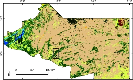
2.1. Study Region
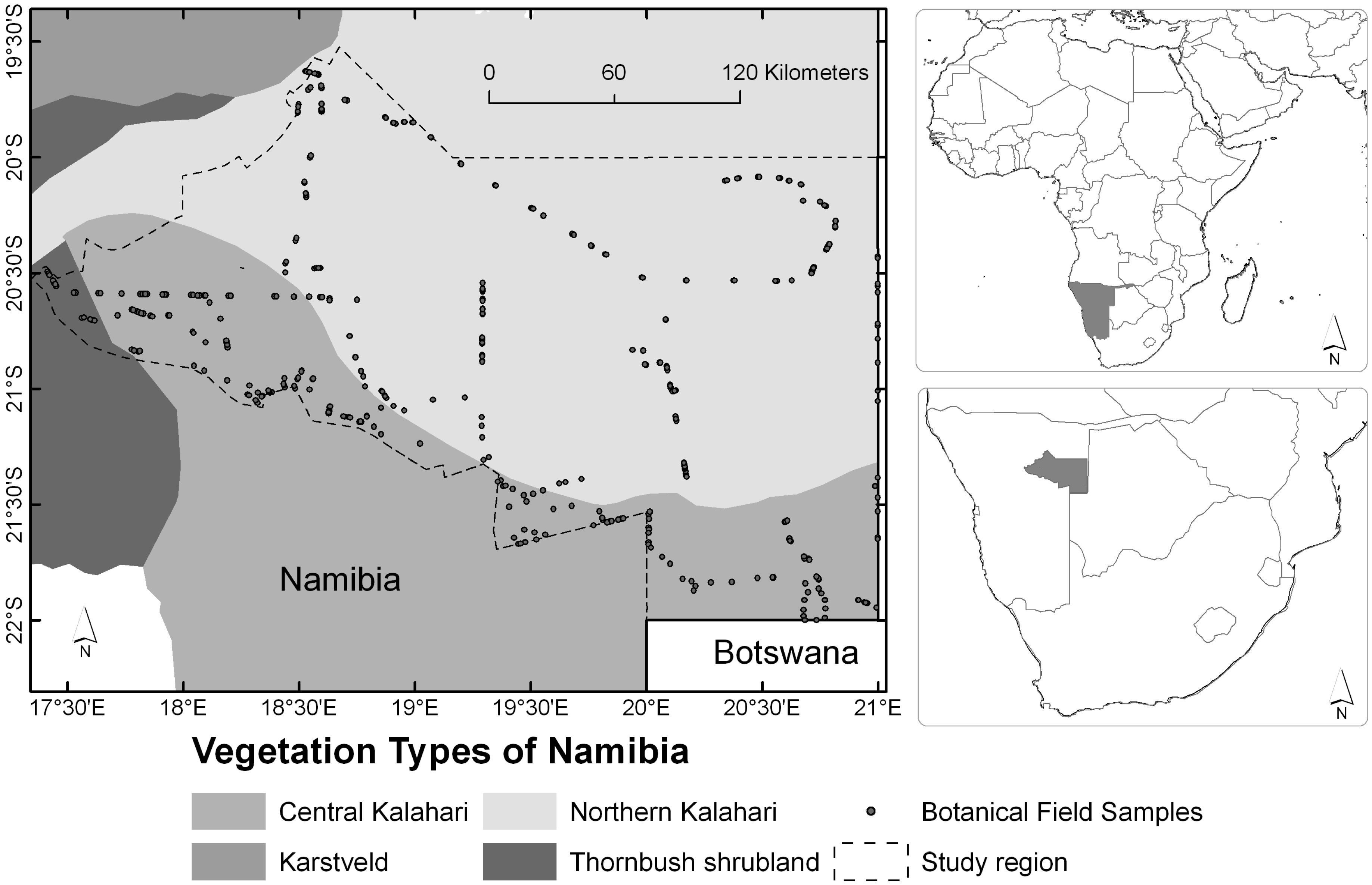
2.2. Field Survey and Vegetetion Data Processing

| Synoptic Vegetation Type Legend | Vegetation structure types after Edward | Cover tree layer [%] | Cover shrub layer [%] | Cover herb layer [%] | No. of relevés | Smpl. size [pixel] | |||
|---|---|---|---|---|---|---|---|---|---|
| Mean | Sd. | Mean | Sd. | Mean | Sd. | ||||
| Pterocarpus angolensis – Burkea africana woodlands (Pa-Ba) | Tall moderately closed bushland | 11.1 | 8.5 | 40 | 7.7 | 40 | 11.6 | 17 | 758 |
| Combretum imberbe – Acacia tortilis woodlands (Ci-At) | Tall semi-open woodlands | 12.3 | 7.5 | 6.7 | 2.9 | 26.7 | 15.3 | 3 | 582 |
| Terminalia sericea – Combretum collinum shrub- and bushlands (Ts-Cc) | Short moderately closed bushland | 3.3 | 4.6 | 40.0 | 9.1 | 34.6 | 12.6 | 212 | 3,500 |
| Acacia erioloba – Terminalia sericea bushlands (Ae-Ts) | Tall moderately closed bushland | 4.6 | 7.0 | 36.7 | 10.5 | 30.8 | 14.3 | 59 | 3,480 |
| Hyphaene petersiana plains (Hp_pl) | Short moderately closed bushlands | 4.8 | 3.8 | 41.9 | 8.0 | 27.5 | 7.6 | 8 | 316 |
| Acacia mellifera – Stipagrostis uniplumis shrublands, Typicum (Am-Su) | High moderately closed shrublands | 2.9 | 4.8 | 40.0 | 11.6 | 33.7 | 14.4 | 87 | 3,834 |
| Enneapogon desvauxii – Eriocephalus luederitzianus short shrublands on calcareous omirimba & pans (Ed-El) | Tall semi-open shrublands | 2.2 | 4.4 | 23.6 | 15.1 | 44.7 | 15.6 | 9 | 568 |
| Acacia luederitzii – Ptichtolobium biflorum floodplains of the Omatako Omuramba (Al-Pb) | Short moderately closed bushland | 10.3 | 5.5 | 31.7 | 14.4 | 21.7 | 9.8 | 6 | 770 |
| Terminalia prunioides thickets (Tp_th) | Tall moderately closed thickets | 18.3 | 7.6 | 38.3 | 10.4 | 28.3 | 12.6 | 3 | 220 |
| Eragrostis rigidior – Urochloa brachyura grasslands (Er-Ub) | Tall semi-open shrubland | 0.4 | 0.7 | 16.1 | 8.3 | 72.9 | 17.5 | 12 | 304 |
| Graminoid Crops (Gr_cr) | – | – | – | – | – | – | – | – | 130 |
| Bare Areas, Hardpans (pans) | – | – | – | – | – | – | – | – | 120 |
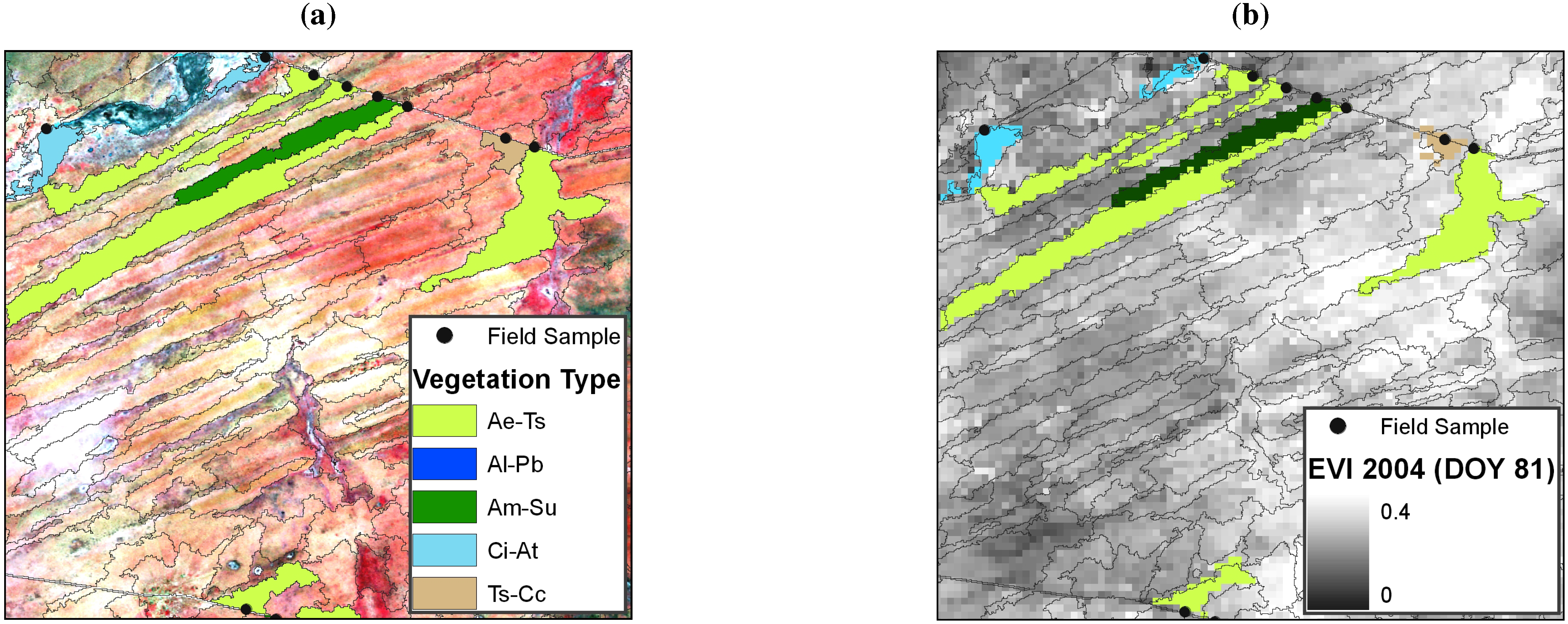
2.3. Satellite Data
2.4. Training Database Generation

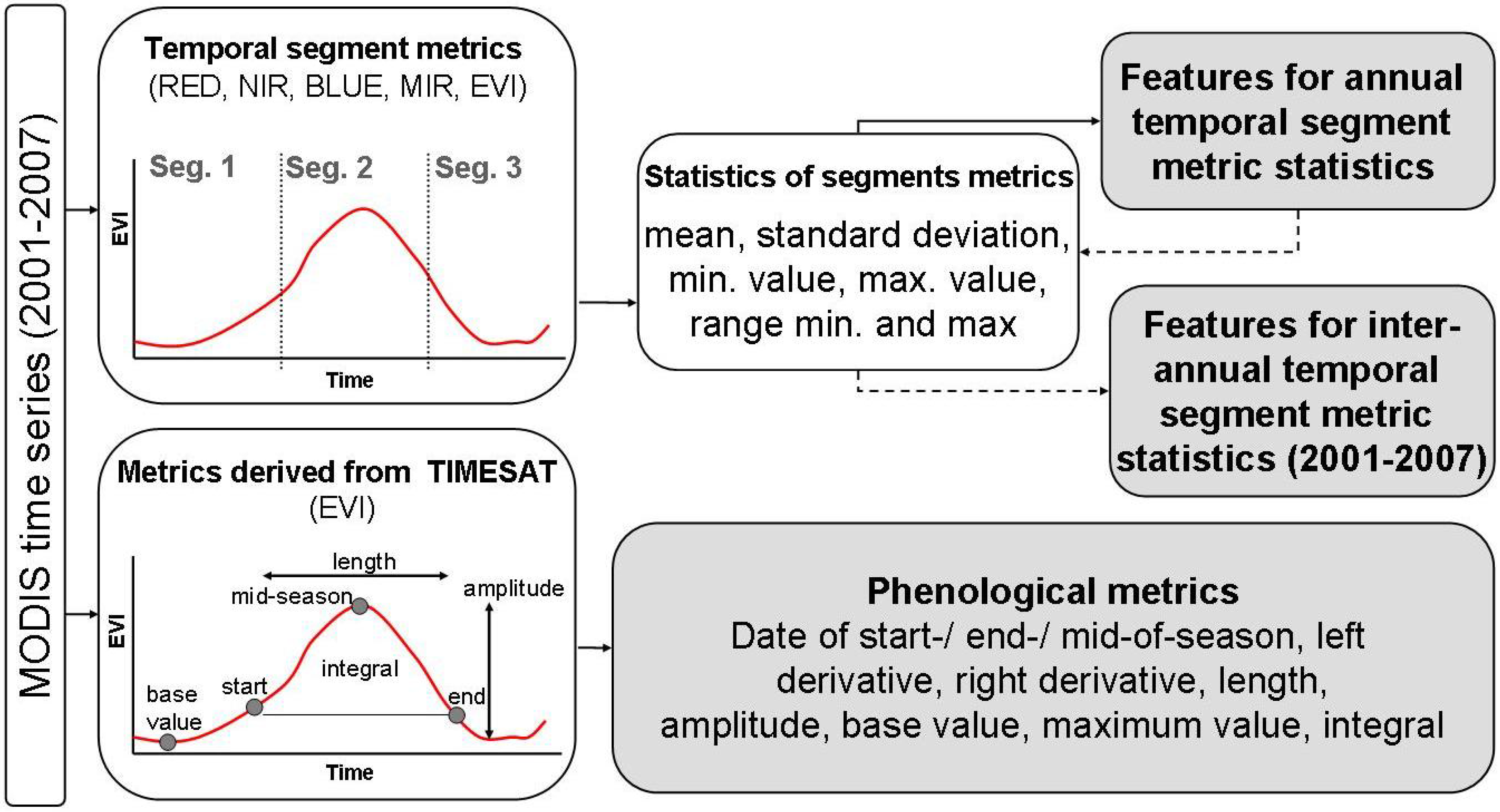
2.5. Calculation of Time Series Metrics

2.6. Separability Analysis
2.7. Random Forest Classification
3. Results
3.1. Suitability of MODIS Time Series Metrics for Semi-Arid Vegetation Mapping

| Inter-annual MODIS segment features 2001-2007 | |||||||||||||
| Gr_cr | Ae-Ts | Al-Pb | Am-Su | Ci-At | Ed-El | HP_pl | Pa-Ba | Tp_th | Ts_Cc | Er_Ub | Pans | ||
| Annual MODIS segment features 2004 | Gr_cr | - | 30.6 | 131 | 31.2 | 191 | 44.8 | 62.3 | 72.2 | 54.5 | 36.9 | 63.8 | 140 |
| Ae-Ts | 3.42 | - | 43.7 | 2.87 | 125 | 7.44 | 33.6 | 23.3 | 25.8 | 5.78 | 30 | 151 | |
| Al-Pb | 13.4 | 6.31 | - | 37.1 | 77.7 | 63.8 | 167 | 140 | 128 | 81.3 | 103 | 146 | |
| Am-Su | 3.49 | 0.31 | 5.94 | - | 124 | 11.8 | 31.8 | 30.5 | 21.8 | 13.5 | 38.7 | 142 | |
| Ci-At | 23.8 | 18.9 | 10.5 | 18.8 | - | 151 | 284 | 211 | 241 | 153 | 120 | 144 | |
| Ed-El | 7.17 | 1.47 | 6.73 | 1.53 | 21 | - | 30.2 | 37.9 | 31 | 12.3 | 44.1 | 155 | |
| HP_pl | 13.3 | 7.03 | 23.1 | 6.89 | 44.2 | 7.5 | - | 79.6 | 48.7 | 41 | 116 | 162 | |
| Pa-Ba | 7.52 | 1.8 | 11.6 | 2.37 | 29.7 | 3.28 | 4.64 | - | 59.2 | 16.9 | 31.6 | 159 | |
| Tp_th | 8.46 | 6.72 | 10.5 | 5.99 | 26.6 | 9.21 | 17.3 | 8.51 | - | 40.8 | 78.6 | 143 | |
| Ts_Cc | 3.78 | 0.2 | 6.25 | 0.24 | 18.3 | 1.42 | 6.43 | 1.61 | 6.3 | - | 27.4 | 162 | |
| Er_Ub | 7.71 | 5.63 | 8.18 | 6.31 | 8.6 | 6.73 | 21.1 | 11.5 | 13.6 | 5.65 | - | 146 | |
| Pans | 15.3 | 14.7 | 17.6 | 14.5 | 15.4 | 16 | 18.8 | 17.6 | 14 | 14.4 | 12.1 | - | |
3.2. Vegetation Type Mapping

3.3. Classification Error Assessment
| class | 2001/02 | 2002/03 | 2003/04 | 2004/05 | 2005/06 | 2006/07 | 2001–2007 | |||||||
| users | prod. | users | prod. | users | prod. | users | prod. | users | prod. | users | prod. | users | prod. | |
| Gr_cr | 50.76 | 91.66 | 52.30 | 93.15 | 59.23 | 100.00 | 48.46 | 98.43 | 62.30 | 100.0 | 45.38 | 100.00 | 93.84 | 100.00 |
| Ae-Ts | 94.10 | 92.29 | 93.93 | 92.64 | 95.53 | 93.02 | 94.64 | 91.10 | 93.50 | 89.49 | 93.47 | 87.42 | 96.35 | 96.18 |
| Al-Pb | 95.84 | 96.72 | 95.97 | 96.72 | 95.58 | 94.72 | 97.14 | 97.01 | 97.14 | 95.16 | 92.33 | 92.45 | 98.96 | 97.94 |
| Am-Su | 92.67 | 89.94 | 92.98 | 89.52 | 94.26 | 91.07 | 92.93 | 91.94 | 92.22 | 90.34 | 90.32 | 90.53 | 96.63 | 95.09 |
| Ci-At | 90.89 | 97.06 | 91.75 | 96.56 | 91.23 | 93.98 | 96.90 | 96.90 | 95.53 | 97.03 | 87.62 | 94.61 | 96.28 | 97.96 |
| Ed-El | 75.52 | 91.86 | 75.00 | 92.40 | 77.81 | 91.32 | 77.81 | 96.71 | 69.71 | 92.74 | 67.78 | 93.67 | 85.03 | 96.60 |
| HP_pl | 92.72 | 97.34 | 94.30 | 98.02 | 90.82 | 97.61 | 93.67 | 95.48 | 92.08 | 97.32 | 91.13 | 94.11 | 97.78 | 96.86 |
| Pa-Ba | 94.19 | 97.01 | 93.27 | 97.11 | 91.95 | 95.74 | 96.04 | 97.32 | 90.50 | 97.86 | 92.48 | 96.42 | 97.22 | 99.86 |
| Tp_th | 81.36 | 96.75 | 81.81 | 98.36 | 91.36 | 99.01 | 96.36 | 99.53 | 82.27 | 98.36 | 90.90 | 99.00 | 95.90 | 100.00 |
| Ts_Cc | 93.34 | 89.09 | 93.11 | 89.28 | 91.85 | 90.03 | 92.22 | 89.71 | 91.37 | 87.97 | 91.88 | 87.22 | 95.48 | 93.48 |
| Er_Ub | 73.35 | 95.70 | 75.00 | 95.39 | 71.71 | 96.88 | 75.65 | 99.13 | 73.02 | 97.36 | 71.38 | 96.44 | 84.86 | 98.85 |
| Pans | 93.33 | 98.24 | 93.33 | 98.24 | 95.83 | 99.13 | 99.16 | 100.00 | 98.33 | 100.00 | 90.83 | 98.19 | 100.00 | 100.00 |
| overall accuracy | 85.67 | 94.47 | 86.07 | 94.78 | 87.26 | 95.21 | 88.41 | 96.11 | 86.50 | 95.30 | 83.79 | 94.17 | 94.86 | 97.73 |
| Kappa | 0.91 | 0.90 | 0.90 | 0.91 | 0.88 | 0.87 | 0.93 | |||||||
4. Discussion
4.1. Requirements for Rainfall Amount for Vegetation Type Mapping
4.2. Spectral and Temporal Requirements for Dry Savanna Vegetation Mapping

5. Conclusions
Acknowledgements
References and Notes
- Strohbach, B. Vegetation Survey of Namibia. J. Nam. Sci. Soc. 2001, 49, 93–118. [Google Scholar]
- Burke, A.; Strohbach, B. Vegetation studies in Namibia. Dinteria 2000, 26, 1–24. [Google Scholar]
- Volk, O. Die Florengebiete von Südwestafrika. J. S. W. A. Sci. Soc 1966, 20, 25–58. [Google Scholar]
- Giess, W. A preliminary vegetation map of South West Africa. Dinteria 1971, 4, 1–114. [Google Scholar]
- Volk, O.; Leippert, H. Vegetationsverhältnisse im Windhoeker Bergland, Südwestafrika. J. S. W. A. Sci. Soc. 1971, 30, 5–44. [Google Scholar]
- Robinson, E. Phytosociology of the Namib Desert Park, South West Africa. M.Sc. thesis, Department of Botany, University of Natal, Pietermaritzburg, South Africa, 1976. [Google Scholar]
- Jürgens, N.; Burke, A.; Sally, M.; Jacobson, K. Desert. In Vegetation of Southern Africa; Cowling, R.M., Richardson, D.M., Pierce, S.M., Eds.; Cambridge University Press: Cambridge, UK, 1997. [Google Scholar]
- Jankowitz, W.; Venter, H. Die plantgemeenskappe van die Waterberg-platopark. Madoqua 1987, 15, 97–146. [Google Scholar]
- le Roux, C.L.G.; Grunow, J.O.; Morris, J.W.; Bredenkamp, G.J.; Scheepers, J.C. A classification of the vegetation of the Etosha National Park. S. Afr. J. Bot. 1988, 54, 1–10. [Google Scholar]
- du Plessis, W.P.; Breedenkamp, G.J.; Trollope, W.S.W. Response of herbaceous species to a degradation gradient in the western region of Etosha National Park, Namibia. Koedoe 1998, 41, 19–28. [Google Scholar] [CrossRef]
- Strohbach, B.; Calitz, A.; Coetzee, M.E. Erosion Hazard Mapping: Modelling vegetative cover. Agricola 1996, 8, 53–59. [Google Scholar]
- Sannier, C.A.D.; Taylor, J.C.; du Plessis, W.; Campbell, K. Real-time vegetation monitoring with NOAA-AVHRR in Southern Africa for wildlife management and food security assessment. Int. J. Remote Sens. 1998, 19, 621–639. [Google Scholar] [CrossRef]
- Colditz, R.; Keil, M.; Strohbach, B.; Gessner, U.; Schmidt, M.; Dech, S. Vegetation structure mapping with remote sensing time series: Capabilities and improvements. In Proceedings of the 32nd International Symposium on Remote Sensing of Environment, San Jose, Costa Rica, June 25–29, 2007.
- Verburg, P.; van de Steeg, J.; Veldcamp, A.; Villemann, L. From land cover change to land function dynamics: A major challenge to improve land characterization. J. Environ. Manage. 2009, 90, 1327–1335. [Google Scholar] [CrossRef] [PubMed]
- Herold, M. A joint initiative for harmonization and validation of land cover datasets. IEEE Trans. Geosci. Remote Sens. 2006, 44, 1719–1727. [Google Scholar] [CrossRef]
- Lambin, E. Monitoring forest degradation in tropical regions by remote sensing: some methodological issues. Global Ecol. Biogeogr. 1999, 8, 191–198. [Google Scholar] [CrossRef]
- Nagendra, H. Using remote sensing to assess biodiversity. Int. J. Remote Sens. 2001, 22, 2377–2400. [Google Scholar] [CrossRef]
- DeFries, R.; Hansen, M.; Townshend, J.; Sohlberg, R. Global land cover classifications at 8 km spatial resolution: the use of training data derived from Landsat imagery in decision tree classifiers. Int. J. Remote Sens. 1998, 19, 3141–3168. [Google Scholar] [CrossRef]
- Steenkamp, K.; Wessels, K.; Archibald, S.; von Maltitz, G. Satellite derived phenology of southern Africa for 1985-2000 and functional classification of vegetation based on phenometrics. In Proceedings of the 33rd International Symposium of Remote Sensing of the Environment (ISRSE), Stresa, Italy, May 4–8, 2009.
- Hansen, M.; DeFries, R.; Townsend, J.; Carrol, M.; Dimeceli, C.; Sohlberg, R. Global percent tree cover at a spatial resolution of 500 meters: first results of the MODIS vegetation contineous fields algorithm. Earth Interact. 2003, 7, 1–15. [Google Scholar] [CrossRef]
- Gessner, U.; Klein, D.; Conrad, C.; Schmidt, M.; Dech, S. Towards an automated estimation of vegetation cover fractions on multiple scales: Examples of Eastern and Southern Africa. In Proceedings of the 33rd International Symposium of Remote Sensing of the Environment, Stresa, Italy, May 4–8, 2009.
- Breiman, L.; Friedmann, J.; Olshen, R.; Stone, C. Classification and Regression Trees; CRC Press: Boca Raton, FL, USA, 1984. [Google Scholar]
- DeFries, R.; Hansen, M.; Townshend, J. Global discrimination of land cover types from metrics derived from AVHRR pathfinder data. Remote Sens. Environ. 1995, 54, 209–222. [Google Scholar] [CrossRef]
- Friedl, M.; Brodley, C. Decision tree classification of land cover from remotely sensed data. Remote Sens. Environ. 1997, 61, 399–409. [Google Scholar] [CrossRef]
- Hansen, M.C.; DeFries, R.; Townshend, J.; Sohlberg, R. Global land cover classification at 1km spatial resolution using a classification tree approach. Int. J. Remote Sens. 2000, 21, 1331–1364. [Google Scholar] [CrossRef]
- Chan, J.; Huang, C.; DeFries, R. Enahanced algorithm performance for land cover classification from remotely sensed data using bagging and boosting. IEEE Trans. Geosci. Remote Sens. 2001, 39, 693–695. [Google Scholar]
- Breiman, L. Random forests. Mach. Learn. 2001, 45, 5–32. [Google Scholar] [CrossRef]
- Pal, M. Random forest classifier for remote sensing classification. Int. J. Remote Sens. 2005, 26, 217–222. [Google Scholar] [CrossRef]
- Chan, J.; Paelinckx, D. Evaluation of random forest and adaboost tree-based ensemble classification and spectral band selection for ecotope mapping using airborne hyperspectral imagery. Remote Sens. Environ. 2008, 112, 2999–3011. [Google Scholar] [CrossRef]
- Watts, J.; Lawrence, R. Merging Random Forest Classification with an object-oriented approach for analysis of Agricultural Lands. The International Archives of the Photogrammetry, Remote Sensing and Spatial Information Sciences 2008, 37, 579–582. [Google Scholar]
- Running, S.; Loveland, T.; Pierce, L.; Nemany, R.; Hunt, E. A Remote Sensing Based Vegetation Classification Logic for Global Land Cover Analysis. Remote Sens. Environ. 1995, 51, 39–48. [Google Scholar] [CrossRef]
- Bonan, G.; Levis, S. Landscapes as patches of plant functional types: An integrating concept for climate and ecosystem models. Global Biochem. Cy. 2002, 16, 1–18. [Google Scholar] [CrossRef]
- Gessner, U.; Conrad, C.; Hüttich, C.; Keil, M.; Schmidt, M.; Schramm, M.; Dech, S. A multi-scale approach for retrieving proportional cover of life forms. In Proceedings of the IEEE International Geoscience and RemoteSensing Symposium, Boston, MA, USA, July 6–11, 2008.
- Herold, M.; Mayaux, P.; Woodcock, C.; Baccini, A.; Schmullius, C. Some challenges in global land cover mapping: An assessment of agreement and accuracy in existing 1 km datasets. Remote Sens. Environ. 2008, 112, 2538–2556. [Google Scholar] [CrossRef]
- Jung, M.; Henkel, K.; Herold, M.; Churkina, G. Exploiting synergies of global land cover products for carbon cycle modelling. Remote Sens. Environ. 2006, 101, 534–553. [Google Scholar] [CrossRef]
- Bicheron, P.; Defourny, P.; Schouten, C.B.L.; Vancutsem, C.; Huc, M.; Bontemps, S.; Leroy, M.; Achard, F.; Herold, M.; Ranera, F.; Arino, O. GLOBCOVER - Products description and validation report, medias France technical documants. Available online at: http://postel.mediasfrance.org/en/DOWNLOAD/Documents/ (accessed May 12, 2009).
- Mendelsohn, J.; el Obeid, S. The Communal Lands in Eastern Namibia; RAISON: Windhoek, Namibia, 2002. [Google Scholar]
- King, L. South African Scenery; Hafner Publishing Company: New York, NY, USA, 1963. [Google Scholar]
- de Pauw, E.; Coezee, M.E.; Calitz, A.J.; Beukes, H.; Vits, C. Production of an Agro-Ecological Zones map of Namibia (first approximation). Part II: Results. Agricola 1999, 10, 33–43. [Google Scholar]
- Strohbach, B.; Strohbach, M.; Kutuahuripa, J.; Mouton, H. A Reconnaissance Survey of the Landscapes, Soils and Vegetation of the Eastern Communal Areas (Otjiozondjupa and Omaheke Regions), Namibia; National Botanical Research Institute and Agro-Ecological Survey Programme Directorate Agriculture Research and Training, Ministry of Agriculture, Water and Rural Development: Windhoek, Namibia, 2004. [Google Scholar]
- Edwards, D. A broad-scale structural classification of vegetation for practical purposes. Bothalia 1983, 14, 705–712. [Google Scholar] [CrossRef]
- Global and National Soils and Terrain Digital Databases (SOTER); Land and Water Development Division, Food and Agriculture Organisation of the United Nations: Rome, Italy, 1993.
- Hennekens, S. TURBO(VEG) Software Package for Input, Processing, and Presentation of Phytosociological Data. User’s Guide; IBN-DLO: Wageningen, The Netherlands, 1996. [Google Scholar]
- Hill, M. TWINSPAN -A FORTRAN Program for Arranging Multivariate Data in an Ordered Two-Way Table by Classification of the Individuals and Attributes; Cornell University: Ithaca, NY, USA, 1979. [Google Scholar]
- Westfall, R.; Theron, G.; van Rooyen, N. Objective classification and analysis of vegetation data. Plant Ecol. 1997, 132, 137–154. [Google Scholar] [CrossRef]
- Justice, C.; Townshend, J.; Vermote, E.; Masuoka, E.; Wolfe, R.; Saleous, N.; Roy, D.; Morisette, J. An overview of MODIS Land data processing and product status. Remote Sens. Environ. 2002, 83, 3–15. [Google Scholar] [CrossRef]
- Colditz, R.; Conrad, C.; Wehrmann, T.; Schmidt, M.; Dech, S. TiSeG: Flexible software tool for time-series generation of MODIS data utilizing the quality assessment science data set. IEEE Trans. Geosci. Remote Sens. 2008, 46, 3296–3308. [Google Scholar] [CrossRef]
- Huete, A.; Didan, K.; Miura, T.; Rodriguez, E.; Gao, X.; Ferreira, L. Overview of the radiometric and biophysical performance of the MODIS vegetation indices. Remote Sens. Environ. 2002, 83, 195–213. [Google Scholar] [CrossRef]
- Satake, M.; Oshimura, K.; Ishido, Y.; Kawase, S.; Kozu, T. TRMM PR data processing and calibration to be performed by NASDA. In IEEE Conference Proceedings, Geoscience and Remote Sensing Symposium, IGARSS ’95, Quantitative Remote Sensing for Science and Applications, Firenze, Italy, July 10–14, 1995.
- Definiens Developer 7 - Reference Book. Definiens AG: München, Germany, 2007.
- Roy, D.; Boschetti, L.; Justice, C.; Ju, J. The collection 5 MODIS burned area product - global evaluation by comparison with the MODIS active fire product. Remote Sens. Environ. 2008, 112, 3690–3707. [Google Scholar] [CrossRef]
- Jönsson, P.; Eklundh, L. TIMESAT - A program for analyzing time-series of satellite sensor data. Comput. Geosci. 2004, 30, 833–845. [Google Scholar] [CrossRef]
- Chaudhuri, G.; Borwankar, J.D.; Rao, P. Bhattacharyya distance-based linear discriminant function for stationary time series. Comm. Statist. 1991, 20, 2195–2205. [Google Scholar] [CrossRef]
- Herold, M.; Hang, L.X.; Clarke, K. Spatial metrics and image texture for mapping urban land use. Photogramm. Eng. Remote Sens. 2003, 69, 991–1001. [Google Scholar] [CrossRef]
- Landgrebe, D.; Biehl, L. An Introduction to MultiSpec; Purdue University: West Lafayette, IN, USA, 1997. [Google Scholar]
- Hastie, T.; Tibshhirani, R.; Friedmann, J. The Elements of Statistical Learning–Data Mining, Inference, and Prediction, 2nd ed.; Hastie, T., Tibshirani, R., Friedman, J., Eds.; Springer: New York, NY, USA, 2009. [Google Scholar]
- Gislason, P.; Benediktsson, J.; Sveinsson, J. Random Forests for land cover classification. Pattern Recogn. Lett. 2006, 27, 294–300. [Google Scholar] [CrossRef]
- Liaw, A.; Wiener, M. Classification and regression by random forest. R News 2002, 2, 18–22. [Google Scholar]
- Hines, C. An ecological study of the vegetation of eastern Bushmanland (Namibia) and its implications for development. M.Sc. thesis, University of Natal, Pietermaritzburg, South Africa, 1992. [Google Scholar]
- Zhang, X.; Friedl, M.; Schaaf, C.; Strahler, A. Monitoring the response of vegetation phenology to precipitation in Africa by coupling MODIS and TRMM instruments. J. Geophys. Res. 2005, 110, 1–14. [Google Scholar] [CrossRef]
- Klein, D.; Roehrig, J. How does vegetation respond to rainfall variability in a semi-humid West African in comparison to a semi-arid East African environment? In Proceedings of the 2nd Workshop of the EARSeL Special Interest Group on Land Use and Land Cover, Bonn, Germany, September 28–30, 2006; Volume 1, pp. 149–156.
- Archibald, S.; Scholes, R. Leaf green-up in a semi-arid African savanna - separating tree and grass responses to environmental cues. J. Veg. Sci. 2007, 18, 583–594. [Google Scholar] [CrossRef]
- Vanacker, V.; Lindermann, M.; Lupo, F.; Flasse, S.; Lambin, E. Impact of short-term fluctuation on interannual land cover change in sub-Saharan Africa. Global Ecol. Biogeogr. 2005, 14, 123–135. [Google Scholar] [CrossRef]
- Childes, S. Phenology of nine common woody species in semi-arid, deciduous Kalahari Sand vegetation. Vegetatio 1989, 79, 151–163. [Google Scholar] [CrossRef]
- Shackleton, C. Rainfall and topo-edaphic influences on woody community phenology in South African savannas. Global Ecol. Biogeogr. 1999, 8, 125–136. [Google Scholar] [CrossRef]
- Sekhwela, M.; Yates, D. A phenological study of dominant acacia tree species in areas with different rainfall regimes in the Kalahari of Botswana. J. Arid Environ. 2007, 70, 1–17. [Google Scholar] [CrossRef]
© 2009 by the authors; licensee Molecular Diversity Preservation International, Basel, Switzerland. This article is an open-access article distributed under the terms and conditions of the Creative Commons Attribution license (http://creativecommons.org/licenses/by/3.0).
Share and Cite
Hüttich, C.; Gessner, U.; Herold, M.; Strohbach, B.J.; Schmidt, M.; Keil, M.; Dech, S. On the Suitability of MODIS Time Series Metrics to Map Vegetation Types in Dry Savanna Ecosystems: A Case Study in the Kalahari of NE Namibia. Remote Sens. 2009, 1, 620-643. https://doi.org/10.3390/rs1040620
Hüttich C, Gessner U, Herold M, Strohbach BJ, Schmidt M, Keil M, Dech S. On the Suitability of MODIS Time Series Metrics to Map Vegetation Types in Dry Savanna Ecosystems: A Case Study in the Kalahari of NE Namibia. Remote Sensing. 2009; 1(4):620-643. https://doi.org/10.3390/rs1040620
Chicago/Turabian StyleHüttich, Christian, Ursula Gessner, Martin Herold, Ben J. Strohbach, Michael Schmidt, Manfred Keil, and Stefan Dech. 2009. "On the Suitability of MODIS Time Series Metrics to Map Vegetation Types in Dry Savanna Ecosystems: A Case Study in the Kalahari of NE Namibia" Remote Sensing 1, no. 4: 620-643. https://doi.org/10.3390/rs1040620