Article

Spectroscopic Analysis of Arsenic Uptake in Pteris Ferns

1
U.S. Geological Survey, Eastern Geographic Science Center, 12201 Sunrise Valley Drive, MS 521, Reston, VA 20192, USA
2
George Mason University, Department of Geography and Geoinformation Science, Fairfax, VA 22030, USA
*
Author to whom correspondence should be addressed.
Remote Sens. 2009, 1(4), 644-675; https://doi.org/10.3390/rs1040644
Submission received: 26 August 2009 / Revised: 22 September 2009 / Accepted: 25 September 2009 / Published: 30 September 2009

Abstract

:
Two arsenic-accumulating Pteris ferns (Pteris cretica mayii and Pteris multifida), along with a non-accumulating control fern (Nephrolepis exaltata) were grown in greenhouse conditions in clean sand spiked with 0, 20, 50, 100 and 200 ppm sodium arsenate. Spectral data were collected for each of five replicates prior to harvest at 4-week intervals. Fern samples were analyzed for total metals content and Partial Least Squares and Stepwise Linear Regression techniques were used to develop models from the spectral data. Results showed that Pteris cretica mayii and Pteris multifida are confirmed hyperaccumulators of inorganic arsenic and that reasonably accurate predictive models of arsenic concentration can be developed from the first derivative of spectral reflectance of the hyperaccumulating Pteris ferns. Both the arsenic uptake and spectral results indicate that there is some species-specific variability but the results compare favorably with previously published data and additional research is recommended.

1. Introduction

Phytoremediation is the removal of contamination by plants. An area of growing technological interest, phytoremediation of contaminated soil offers distinct advantages over traditional techniques because it is inexpensive and far less disruptive to the community and the landscape than the standard soil excavation and replacement. Phytoremediation of fugitive arsenic in soils has recently been utilized in several hazardous waste cleanup efforts and is the result of the discovery that many ferns of the Pteris taxa are hyperaccumulators of inorganic arsenic [1,2,3,4]. The Chinese Brake Fern (Pteris vittata), the Spider Brake Fern (Pteris multifida), the Cretan Brake Fern (Pteris cretica mayii) and several other Pteris ferns have been shown to uptake so much inorganic arsenic in soils that they can actually reduce the soil arsenic concentration of a moderately contaminated site to acceptable levels in just a few growing seasons [5,6].
The spectral reflectance of vegetation growing in soils containing heavy metals has long been a topic of remote sensing investigation and the spectral analysis of ferns that hyperaccumulate arsenic in plants is an especially interesting application of this form of remote sensing. Early laboratory spectroscopic and remote sensing imaging research successfully identified spectral signatures of heavy metal stress and applied these techniques to applications involving mineral prospecting and environmental contamination [7,8,9,10].
Measurement of inorganic arsenic in the soil and in the biomass of plants requires expensive, invasive and time-consuming laboratory chemical methods. The ability to quantify arsenic uptake and removal from the soil through the spectral reflectance of Pteris ferns would be a potentially important new hazardous waste monitoring technique and a valuable addition to the tools of geographic analysis and monitoring. This paper reports on research investigating the controlled measurement of arsenic uptake in two Pteris ferns as well as the feasibility of predicting arsenic concentration in these ferns by way of modeling and analyzing the reflective spectroscopic data in a controlled laboratory environment.

2. Background

2.1. Spectroscopy and Remote Sensing
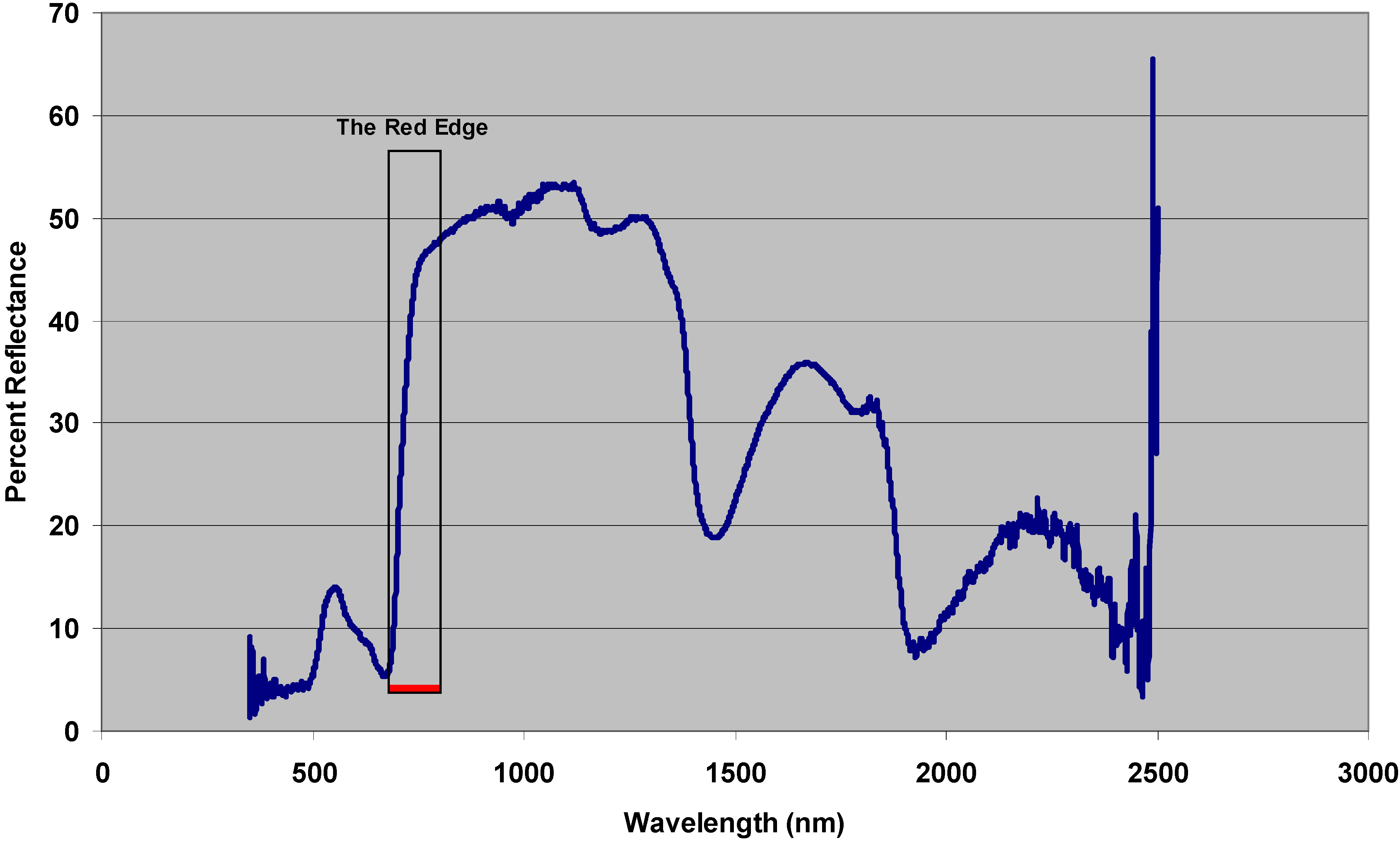
There is a rich history of remote sensing research in evaluating vegetation conditions, such as biomass productivity, disease and stress. Both in the laboratory and from airborne imaging applications, much research has centered around identifying the key wavelengths of the solar reflected part of the electromagnetic spectrum (EMS) for vegetation and gaining a better understanding of how energy interacts with vegetation pigments and leaf structure under different conditions. Laboratory spectroscopic methods generally employ instruments and methods that record reflected energy in very, narrow specific wavelengths. Although closely related to imaging spectroscopy, sometimes called hyperspectral remote sensing, and sensors such as NASA’s AVIRIS (Advanced Visible InfRared Imaging Spectrometer), these methods do not produce imagery, but instead produce spectra, a graphical plot of the record of energy interactions at specific wavelengths.
The use of laboratory spectral reflectance methods to gain an understanding of photosynthesis and related vegetative processes is a field of scientific study that has been ongoing for decades. Laboratory instruments called spectrometers, spectrophotometers, spectrographs or spectroradiometers are all different names for instruments that essentially use some type of prism to separate light into its component parts and measure the reflectance and absorption of those component parts from a target surface. Early instruments separated light into the basic colors of the spectrum. Modern instruments separate light into individual nanometers of reflectance energy.
Spectral research of vegetation actually dates back to the 19th Century. Using a hand held spectrograph, in 1879 Rood analyzed typical vegetation and reported a low reflectance in the blue, a high reflectance in the green, a low reflectance in the red and a rapid rise in reflectance in the infrared [11]. In 1918, Willstatter and Stoll (as documented by Murtha, 1997 [12]) investigated the interaction of light with the typical structure of the leaf using selective spectral absorption [12]. In 1929 Schull studied and measured the reflectance of various leaves using a prism spectrophotometer to attempt to better explain leaf-energy interactions that occur in photosynthesis. Measuring between 430 and 700 nanometers (nm), at roughly 20 nm intervals, he was able to determine the basic chlorophyll absorption pattern of most green vegetation and even reported the common chlorophyll absorption well at 680 nm [13]. McNicholas (1931), through laboratory methods, defined the spectral characteristics of carotin and xanthophyll, and the absorption changes that occurred during oxidation [14].
The spectral characteristics of vegetation have enjoyed a wide range of interest through the years for military, agricultural and environmental applications. Key papers by Gates and others in 1965 [15] and Guyot and others in 1992 [16] summarize the diverse applications of laboratory spectral research for vegetation studies. All green vegetation shows a similar pattern of spectral reflectance in the visible and near infrared regions. The bimodal reflectance pattern is caused by the chlorophyll absorption of blue and red wavelengths, at about 450 nm and 680 nm respectively, and by the reflectance of chlorophyll in the green wavelengths causing the peak at around 550 nm. The second larger spectral peak around 780 nm is caused by the internal structure of leaf tissue that reflects significant amounts of energy in the near infrared. This internal mesophyll tissue generally consists of irregularly shaped cells separated by interconnected openings. Infrared radiation is strongly scattered by this structure, which combined with a general decrease in pigment absorption at the edge of the visible portion of the spectrum, causes a significant increase in reflected energy at the edge of the infrared part of the spectrum. See Figure 1.

2.2. The Red Edge

One of the fundamental concepts that has been developed in the spectral analysis of vegetation has been the “Red Edge” of vegetation reflectance. An area usually centered around the 720 nm area and represented by the typical sharp rise in reflectance in the 680–760 nm range of the classic vegetation spectral signature. The location, size, shape and shifts in this Red Edge form one of the central concepts in spectral monitoring of vegetation condition. Vegetation undergoing stress from exposure to fugitive arsenic in the soil is very likely to exhibit symptoms of that stress in the Red Edge region.
Although the general concept of the Red Edge is easily understood as the area of the sharp rise in reflectance, a variety of definitions and quantitative methods for computing the Red Edge are found in the literature. In 1993, Ray et al. defined the Red Edge as the sharp transition between absorption by chlorophyll in the visible wavelengths and the strong scattering in the near infrared from the cellular structure of leaves [17]. The Red Edge (λ re) was defined by Horler and others in 1983 as the wavelength of maximum ΔR/Δλ, where R is reflectance and λ, is the specific wavelength [18]. Guyot et al. defines the Red Edge as an inflection in the sharp rise in reflectance between 670 nm and 760 nm [16].
Horler and others have studied the feasibility of utilizing a Red Edge measurement as an indication of plant chlorophyll status [18]. Using derivative reflectance spectroscopy in the laboratory, plant chlorophyll status and Red Edge measurements were made of single leaves of several different species. By using spectroscopic and laboratory methods to measure the chlorophyll content of the same leaf samples, direct evidence of the correlation between the Red Edge and chlorophyll concentration was obtained. Ray and others discovered significant differences in the size and shape of the Red Edge in different types of arid vegetation and found that for a common yellow grass species, there was no chlorophyll “bump” and no detectable Red Edge [17].
Figure 1. A spectral plot of typical green vegetation. The highlighted area is known as the “Red Edge”.
Remotesensing 01 00644 g001
Another critical analytical feature of spectral analysis of vegetation is the shift in absorption and reflectance features that occur as a result of chemical and nutrient exposures. A general relationship between increases in chlorophyll concentration and a “red shift” towards longer wavelengths has been established by several researchers. Gates and others showed the basic relationship between the increased chlorophyll and plant health and the shift of the Red Edge towards longer wavelengths. Guyot et al. similarly showed that the Red Edge inflection point shifts to longer red wavelengths as chlorophyll concentrations increase [15,16]. This general correlation between chlorophyll content and red shift was confirmed by Horler and others and Baret et al. for different crop species [18,19].
More important to arsenic effects research however, is the “blue shift” of vegetation spectra that occurs when vegetation has undergone stress from some mineral or chemical agent. Collins and others showed a basic blue shift in conifers affected by metal sulphide in the 700 – 780 nm region [20]. Horler and others found similar blue shifts in tree species subjected to heavy metal concentration in the soil [21]. Similar blue shift results have been reported by Schwaller and Tkach [22] and Milton et al. [8,10].
Rock et al. demonstrated a 5 nm blue shift in spruce and fir species in Vermont and Germany as a result of stress caused by airborne acid deposition [9]. Horler and others studied the effects of heavy metals on the reflectance spectra of plants. Utilizing both natural vegetation growing in known areas of metal concentrations, and specific greenhouse experiments, they established relationships of metal stress to total chlorophyll, chlorophyll a/b ratios, and reduced reflectance at specific wavelengths [9]. Controlled experiments with pea plants and other species showed that the general effect of exposure to cadmium (Cd), copper (Cu), lead (Pb) and zinc (Zn) was growth inhibition. The pea plants also showed changes in the leaf chlorophyll a/b ratios for exposure to Cd and Cu but showed no changes for Pb and Zn. Metal-treated plants in both controlled and natural environments showed a decrease in reflectance at 850 nm, 1,650 nm and 2,200 nm and an increase at 660 nm. Metal concentration in the soil has strong negative correlations to reflectance at 1,650 nm and 2,200 nm and strong positive correlations at 660 nm [9].
More recently, much work has been done on the spectroscopy and hyperspectral image analysis of mine wastes and the acidic, mineral and metal content of those wastes waters and precipitates. Many mining areas in both the eastern and western portions of the United States have been mined for coal, gold, silver, lead and zinc, often leaving waste rocks and tailings rich in pyrite and other sulfides, as well as arsenic, lead and other heavy metals, many of which meet the criteria for hazardous waste [23,24]. Acidic water, the result of sulfide oxidation, can precipitate a large variety of secondary Fe-bearing minerals whose pH is typically near-neutral or highly acidic depending on a number of oxidation and/or moisture-related variables. Both field and imaging spectroscopic analysis has the ability to identify specific minerals and their relative acidity.
In several key papers from 2001 to 2004, several researchers in The Netherlands successfully demonstrated the use of spectroscopic techniques for indentifying heavy metal and hydrocarbon contamination in river floodplains [25,26,27,28]. Kooistra et al. [27] and Clevers et al. [28] showed that the spectral response of vegetation reflectance could be used to establish quantitative relationships with elevated heavy metal contamination of Ni, Cd, Cu, Zn and Pb in the soil.
Rosso et al. [29] showed that the spectral characteristics of marsh vegetation stress were significantly correlated with symptoms of cadmium and lightweight petroleum contamination, and had a distinct signature for both types of contaminants. Schuerger et al. [30] modeled zinc stress in bahia grass in controlled conditions and showed that NDVI and several other vegetation indices could be used to model zinc stress at certain levels. Sridhar et al. [31] exposed Pteris vittata ferns to arsenic and chromium soil contamination in a controlled environment and found that a unique ratio of R1110/R810 monitors structural changes in the fern due to Cr accumulation was not as successful in the As treated ferns. This study suggests that the infrared reflectance spectrum in the 800 – 1,300 nm range may provide a unique, non-intrusive monitoring method to access the physiological status of plants grown in heavy metal-contaminated soil.

2.3. Arsenic and Arsenic Phytoremediation

Arsenic is a major contamination problem around the world. It is a naturally occurring element that has been known to be highly toxic to human health since Greek times. Arsenic is toxic at very low doses and the current EPA action level for arsenic removal from soil is only 43 parts per million (ppm) (CERCLA 1980 [32]). Although it has been used throughout history in various medicinal purposes, it is generally associated with its toxicity and killing powers, having gained nicknames like “the inheritance powder” in France and has been one of the most popular substances used in malevolent poisonings up through the 19th Century [33]. Arsenic is a by-product of many mining processes and has been used extensively in pesticide industry and, until recently, was used widely as a wood preservative [34].
Although it is often associated with heavy metals, Arsenic is classified as a transition element and a metalloid, reflecting the fact that it commonly forms complexes with metals. It also readily reacts to form covalent bonds with carbon, hydrogen and oxygen. Because of these chemical properties, arsenic readily bonds to soil, especially soils that contain iron.
Arsenic is a major contaminant of soils and waters in the United States and other countries. Contamination of surface water, ground water, and drinking water by arsenic poses significant health risks to humans and animals. Arsenic is a known carcinogen and mutagen, is detrimental to the immune system, and contributes to skin, bladder, and other cancers [35]. According to the U.S. Geological Survey, in 24% of the counties in the United States where data are available, at least 10% of samples have arsenic concentration in water exceeding 10 parts per billion (ppb), the World Health Organization’s arsenic limit in drinking water [36]. Approximately 6% of the US small public water-supply systems had water arsenic concentrations exceeding 10 ppb, and 1% of such systems had concentrations exceeding 50 ppb, the current US maximum limit of arsenic in drinking water [36]. In some parts of the world, arsenic occurs naturally in groundwater. For example, a recent survey indicates that 80% of total area, and 40 million people, are at risk of arsenic poisoning in Bangladesh, where more than 7,000 patients are seriously affected by arsenic in drinking water [37].
Arsenic is a naturally occurring element in rocks, soils, and the waters in contact with them. Before 1968, inorganic forms of arsenic were used extensively in agriculture as insecticides and herbicides. Frequent application at high rates of these chemicals caused significant arsenic accumulation in orchard soils. Inorganic forms of arsenic have since been replaced with organic forms because of their reduced phytotoxicity and overall environmental burden. However, excessive additions of any arsenic compounds can cause pollution of nearby ground and surface waters [38]. Arsenic concentrations as high as 500 mg/kg have been reported in soils having a history of arsenic pesticide or herbicide applications. Such arsenic contaminated soils become a source of contamination in surface water, ground water, and drinking water. Fugitive environmental arsenic is still produced today as a result of various mining, industrial and manufacturing operations [34].
Phytoremediation is the process of removing contaminants from the environment using plants. In general, when plants uptake water and nutrients from the soil, they also sometimes uptake hazardous chemicals or metals where they are stored in the plant tissues, reduced to less dangerous forms or changed into gases and released into the air.
Plants can also aid cleanup by sorbing hazardous materials to their roots or reducing chemicals to less dangerous forms as a result of microbial or bacterial action from the plant roots [39]. Phytoremediation is most often used to remove contaminants from soils, but has also found applications in air and for groundwater [39,40,41] is an attractive alternative to conventional soil removal and replacement techniques because it is a natural process that does not disturb the landscape, it does not potentially expose workers to dangerous substances, and, it is generally much more cost-efficient [39].
In 2001, the Chinese Brake Fern (Pteris vittata) was shown to hyperaccumulate inorganic arsenic in soils [1]. Although there are other plants that are known to hyperaccumulate metals, the Chinese Brake is the first embryophyte (land plant) to hyperaccumulate arsenic and store it in the leaf cells and with its relatively large biomass, it instantly became a model for phytoremediation of one of the world’s major soil contaminants [42]. Since the original discovery of the Chinese Brake Fern, several other ferns from the Pteris family have also been found to be hyperaccumulators of inorganic arsenic [4].

3. Materials and Methods

3.1. Plant and Soil Conditions

In order to identify any potential spectral signature, index, shift or other spectral observable that was linked to, and was predictive of, arsenic stress and/or arsenic uptake during phytoremediation, two arsenic-hyperaccumulating varieties of Pteris ferns (Pteris cretica mayii and Pteris multifida) and common Boston fern (Nephrolepis exaltata), used for control, were grown in a controlled laboratory environment under contract to Edenspace Incorporated (Chantilly, Virginia), the holder of the patent on phytoremediation of arsenic with ferns.
Figure 2. The ferns used in this experiment: A) Pteris cretica mayii, B) Pteris multifida, C) Nephrolepis exalta, D) all ferns growing in the greenhouse. Figures A, B and C used by permission of Heaton’s Nursery, Australia.
Remotesensing 01 00644 g002
From April to October 2004, 300 individual ferns were grown in soils amended with varying levels of sodium arsenate to achieve five general soil concentrations of arsenic from 0 to 200 ppm [43]. See Figure 2. Plants were harvested every four weeks, dried and sent to a commercial chemistry laboratory for analysis of total metals. Spectral reflectance data were collected with an Analytical Spectral Devices (ASD, Boulder, Colorado) Full Range spectrometer for each plant just prior to harvest.
Twenty individual sporelings from each variety were transplanted in 10 cm pots of each of five soil-arsenic concentrations. The soil consisted of clean, homogeneous sand spiked with sodium arsenate to achieve approximate concentrations of 0, 20, 50, 100 and 200 ppm. The sand was limed to achieve a neutral pH of 7 and fertilized to 100 ppm nitrogen, 50 ppm phosphorous and 100 ppm potassium plus other micronutrients. The soil medium was equilibrated for two wetting and drying cycles to homogenize the arsenic and fertilizer mixtures. Weekly fertilizer supplements were provided using a 0.025-0.025-0.025 (Nitrogen-Phosphorous-Potassium plus micronutrients) solution applied as part of the regular watering schedule [43]. Samples from each of the five concentration batches were collected for laboratory analysis by USEPA 3050 method for total metals [44]. The analysis showed final, pre-concentrations of < 2.5, 18, 34, 64 and 183 ppm, respectively [43]. As a final test, spectra were collection from ferns being utilized in a phytoremediation field test and evaluated using laboratory analysis and the models developed to predict arsenic concentration.

3.2. Spectral and Chemical Data Collection

Four replicates of each fern and arsenic soil concentration were harvested on a four week schedule between weeks 4 and 20. Reflectance spectra of ferns were collected just prior to each four week harvest using the ASD full range (400 – 2,500 nm) spectroradiometer. This instrument utilizes grating prisms, three separate detector arrays and fiber optics to collect reflected energy in the 400 – 2,500 nm range, known as the “solar reflected” part of the EMS. The spectral resolution of this instrument is 1 nm. A Dell Latitude C640 laptop computer was connected to the spectrometer and used to execute the spectral collection instrument software. The fiber optic cable of the spectrometer is housed in a pistol grip assembly and mounted on a standard camera tripod to be perpendicular to the target. Spectra were calibrated against a white Spectralon surface and processed according to standard techniques [45]. A Lowell lamp was used as a light source for all spectral collections and was mounted on a 60 degree angle to the spectral target. See Figure 3.
Figure 3. Spectral data collection in the laboratory.
Remotesensing 01 00644 g003
Spectra for each individual fern in each of the three species was summarized in spreadsheets showing the laboratory control values, plant dry weight, arsenic concentration, arsenic content in plants and the 2,151 spectral values representing 1 nm wavelength increments of the solar visible wavelength range of 350 – 2,500 nm.
Four replications of each fern variety were harvested at 4-week intervals after transplanting for a total of 20 weeks (4, 8, 12, 16 and 20 weeks). The plants were harvested by cutting the above ground material 2.5 cm above the soil surface. The vegetation samples were oven dried at 85 °C for 24 hours and the dried samples were weighed and shipped to a commercial laboratory and analyzed for total metals by Inductively Coupled Plasma / Atomic Emission Spectroscopy (ICP/AES) methods.

3.3. Statistical/Analytical Techniques: PLS and SLR

The statistical analysis of the relationship between the spectral reflectance of the ferns and their corresponding biomass arsenic concentration were conducted with three statistical methods including simple correlation analysis and two multivariate techniques; partial least squares (PLS) regression and stepwise linear regression (SLR). All statistical analyses were conducted with SAS, version 9.0 (The SAS Institute, Apex, NC, USA) software. For each spectral collection, PLS and SLR techniques were investigated for the raw reflectance and both the first and second derivatives. Because of the highly correlative nature of hyperspectral data, analysis presents special statistical problems with autocorrelation and these two statistical techniques, PLS and SLR, have emerged in the literature as successful approaches for the analysis of hyperspectral data, especially as it relates to vegetation [27,46,47]. These methods were used to develop linear and predictive models of the relationship between plant reflectance and plant arsenic concentration.
The analysis of spectra reflectance data presents unique problems for standard multivariate techniques because of the large numbers of independent variables (>1,500 spectral bands) and the highly correlated nature of those variables, which stems from the fact that each individual spectral band is only 1 nm away from the spectral bands above and below it. The result is that each spectral band records an energy pattern that is very similar to its neighboring bands and is thus highly correlated. Highly correlated independent variables create a condition known as collinearity, which violates the assumptions of linear regression. To develop a predictive and effective linear model, variables must be independent. The overall result of a collinearity condition is that correlated independent variables have unstable coefficients, and although the model developed may have a high R2 value and low residuals, it will perform poorly outside of the immediate data set that was used to develop it.
Partial least squares was first introduced by Swedish mathematician Herman Wold [48] as an exploratory analysis technique in the field of econometrics and was specifically designed to help researchers in situations of small, non-normally distributed data sets with numerous but highly correlated explanatory variables. General PLS and all of its variants consist of a set of regression and classification tasks as well as dimension reduction techniques and modeling tools. Sometimes called a “soft” modeling technique, the strength of PLS resides in its relaxation, or “softening” of the distribution, normality and collinearity restrictions that are inherent in standard multiple linear regression techniques [49].
The underlying assumption of all PLS methods is that the observed data are generated by a system or process which is driven by a small number of latent (not directly observed or intuitive) variables. Projections of the observed data to its latent structure by means of PLS is a variation of principal component analysis (PCA). PLS generalizes and combines features from PCA and multiple regression and is similar to Canonical Correlation Analysis (CCA) in that it can also relate the set of independent variables to a set of multiple dependent response variables and extract latent vectors with maximum correlation [50,51].
PLS is one of a number of covariance-based statistical methods which are often referred to as structural equation modeling or SEM. Also known as a “latent variable” approach to modeling the covariance structures, the PLS model attempts to find the multidimensional direction in the X space that explains the maximum multidimensional variance direction in the Y space. According to its developer, Herman Wold, the term “PLS” is also and more correctly termed “Projection to Latent Structures” [52,53]. Wold’s son, Svante, has been largely responsible for the development and widespread use of PLS methods in the field of chemometrics and chemical engineering [54]. PLS techniques have been successfully applied to industrial process control [55,56]. It has also been used successfully in the study of spatial pattern analysis of imagery of human brain functions [57,58]. More recently, in the field of landscape ecology, PLS has been used to describe how structural variation in landscape metrics are related to biological and chemical properties of surface water [59].
PLS is also used as an exploratory/data mining and analysis tool in remote sensing. As a relatively new technique, the full utilization of PLS is still evolving but it is clear that it has a major application in several types of spectral, remote sensing analyses, due to the large numbers of potential predictive variables and the highly correlated nature of hyperspectral reflectance and hyperspectral imaging data. Kooistra and others used two spectral VIs, the Difference Vegetation Index (DVI) and the Red Edge Position (REP), along with PLS regression to predict the level of metal contamination in the soil based on the spectral reflectance of grasses [27].
The overall goal of PLS processing of spectral data in this study is the reduction of 2,151 variables (bands 350-2,500) down to a manageable number of variables (~100) that have a high probability of significance in a predictive model. The PLS regression produces a number of significant factors using a “leave-one-out” cross-validation method [60]. At several stages in the PLS process, diagnostic checks are performed, sometimes graphically, to help isolate variables for deletion in the model that do not have any significant predictive value or are outliers. The end result of a PLS run is a Variable Importance for Projection (VIP) table. The VIP represents the value of each variable in fitting the PLS model for both predictors and responses. The VIP for each factor is defined as the square root of the weighted average times the number of predictors. If a predictor has a relatively small coefficient (in absolute value) and a small value of VIP, then it is a prime candidate for deletion [60].
Variables with VIP values less than 0.8 and outliers are dropped from the variable list. The VIP table results are then typically divided into four to nine groups. The PLS analysis process is then repeated on the individual groups of variables. Typically the process is iterated two to five times until a manageable subset of variables can be identified based on the top VIP scores in each group and some a priori knowledge of the process being modeled. PLS can itself be used to construct a predictive model but has some drawbacks. One of the strengths of PLS is its relaxation of collinearity and distribution assumptions but this also can result in a set of collinear or redundant independent variables. Also, the best combinations of variables are not necessarily reflected in the VIP table values.
In spectral applications, a common practice is to take the final subset of variables and then place them into a SLR model. The stepwise method is a modification of the forward variable selection technique and differs in that variables already in the model do not necessarily stay there. A SLR model computes the F-statistic for each variable and contains parameters for significance levels for variables to ENTER and to STAY in the model. The SLR process computes all possible combinations of linear variables and ends when none of the variables outside the model has a significance (p-value) at or below the ENTRY level and every variable in the model is significant at the STAY level. Using these sigma-restricted parameterization and general linear model methods, the SLR process simply regresses all possible combinations of input variables and returns the model with the best regression coefficient and the lowest residuals [59].
This combination of PLS and SLR techniques was the primary analytical method used to develop predictive models of arsenic concentration in plants from spectral reflectance data. Analysis was conducted for all three fern species and the PLS procedure was used to reduce the number of potential predictive variables. These variables were input into a SLR model which then developed and optimized a linear regression model.

3.4. Statistical/Analytical Techniques: Derivative spectra

One of the key concepts in the analysis of spectral phenomena is the ability to extract hidden absorption and reflectance features based on the use of derivative functions of the polynomial spectral curve. In situations where the expression of vegetation stress or arsenic uptake may be only a very subtle spectral feature, derivatives can play a critical role in isolating and identifying those types of subtle, but critical features. The derivative is a basic concept from calculus that is defined as the limiting value of the rate of change of a process. At any point on a curve, the y value is changing with respect to x and the derivative is often defined, in its simplest terms as the change in y over the change in x, or Δy/Δx. In spectroscopy, the derivative is often defined as ΔR/Δλ, where R is the reflectance and λ is a specific wavelength. The ΔR/Δλ function is often called the first derivative and subsequent or higher derivatives are created from simply repeating the process.
Many researchers have utilized derivatives to bring out useful features in spectral analyses. Martin et al. [61] used the first difference spectra of forest canopies to identify species based on the specific patterns of nitrogen and lignin concentrations in the leaf. Chen et al. [62] used derivative reflectance spectroscopy to estimate suspended sediment concentrations and found that the derivative relationship was much less affected by environmental/atmospheric variables than the direct spectra record. Demetriades-Shah and others [63] showed that derivative spectral indices were superior to broad-band measures, such as NDVI, for monitoring chlorosis in vegetation. Tsai and Philpot [64] showed that derivatives could be used to minimize the effects of atmospheric conditions. Derivatives have been used extensively in analytical chemistry to reduce the effects of background noise and resolve overlapping spectra. The first derivative has often been used to isolate the specific Red Edge inflection point in vegetation spectra [18]. Wessman and others [65] and Yoder and Pettigrew-Crosby [66] used the first derivative of hyperspectral reflectance data to investigate canopy chemistry such as nitrogen and lignin.
Derivatives of a second order or higher can be valuable for analysis of hyperspectral remote sensing data because they are relatively insensitive to variations in illumination, sun angle, cloud cover and topographic shadow [63]. Kosmas et al. [67] used the second derivative of reflectance spectra for the analysis of iron oxide minerals. Adams and others [68] developed a yellowness index as a measure of chlorosis, which approximated the second derivative and correlated well with NDVI measurements from Advanced Visible InfraRed Imaging System (AVIRIS) data. Chen et al. [69] developed a derivative-based green vegetation index (GVI) that showed a greatly enhanced ability to estimate green cover levels and minimize the effect of background noise. All spectra are essentially sets of x, y pairs that represent energy interactions against some scale of magnitude. For imaging spectroscopy applications, the x variable is wavelength and the y variable is radiance or percent reflectance. Dixit and Ram [70] defined the first order derivative as the change in y over the change in x, or simply, Δy/Δx, and can be computed for spectral data with the formula:
Δy/Δx = (yi-1 – yi) / (xi-1 – xi)
that determines the complete first derivative when applied to all the pairs in the spectra. The same formula, when applied to the results of the first derivative, results in the second derivative and so on.
Analysis of derivative data can be approached in much the same way as direct spectral measurements. Values for specific band locations, such as R680 can be calculated for the first-, second- and nth-order derivatives. Also, spectral features of the derivative graph, such as the wavelength maximum and minimum reflectance can be evaluated. The spectral effects of arsenic on cover vegetation and in the phytoremediation applications are generally unknown and the use of derivatives, along with statistical tools, may help to isolate, or even quantify, the level of arsenic exposure and/or uptake. Derivatives were employed in the analysis of the spectral data for the arsenic accumulating and control ferns in this study.

4. Results

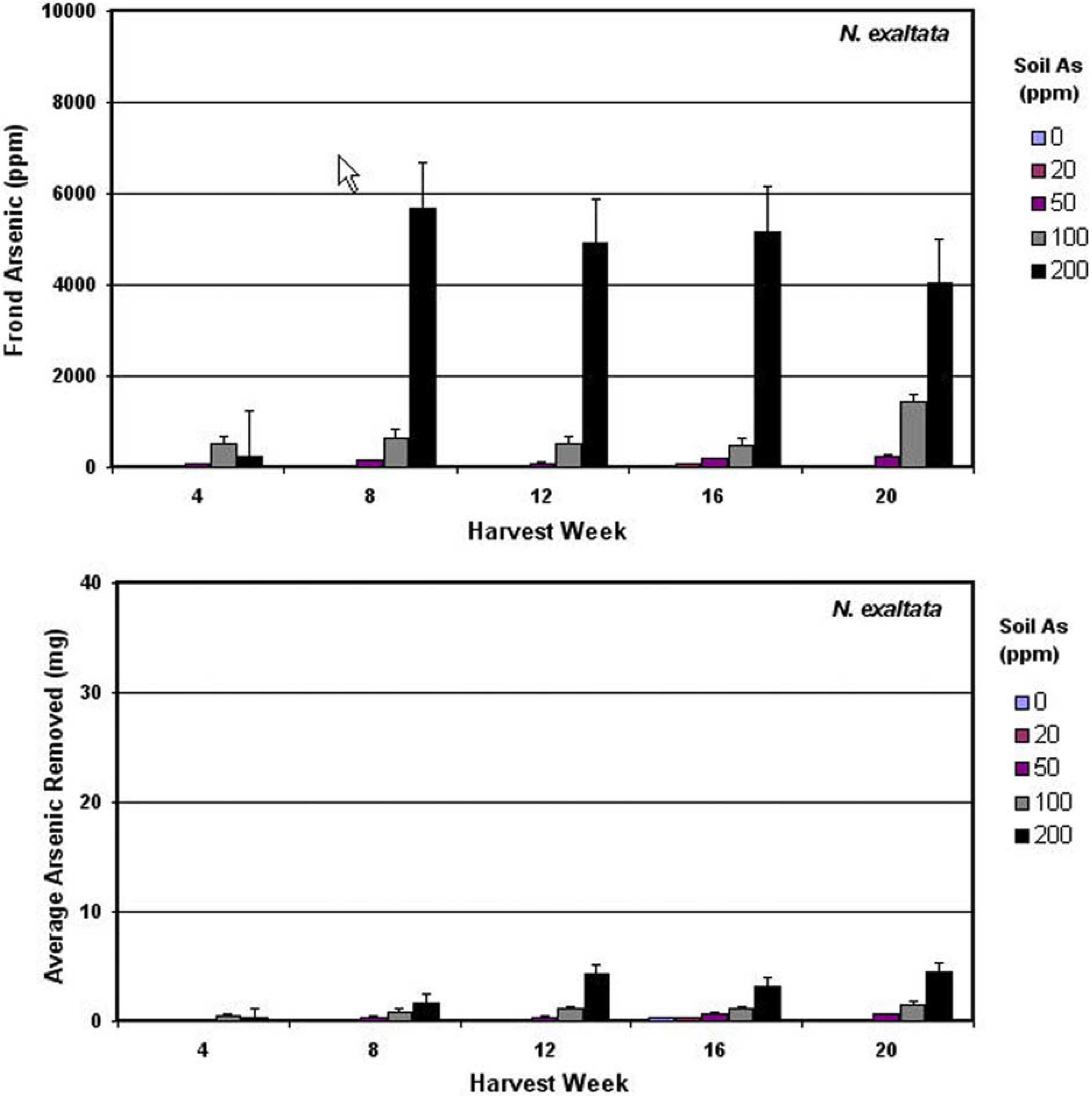
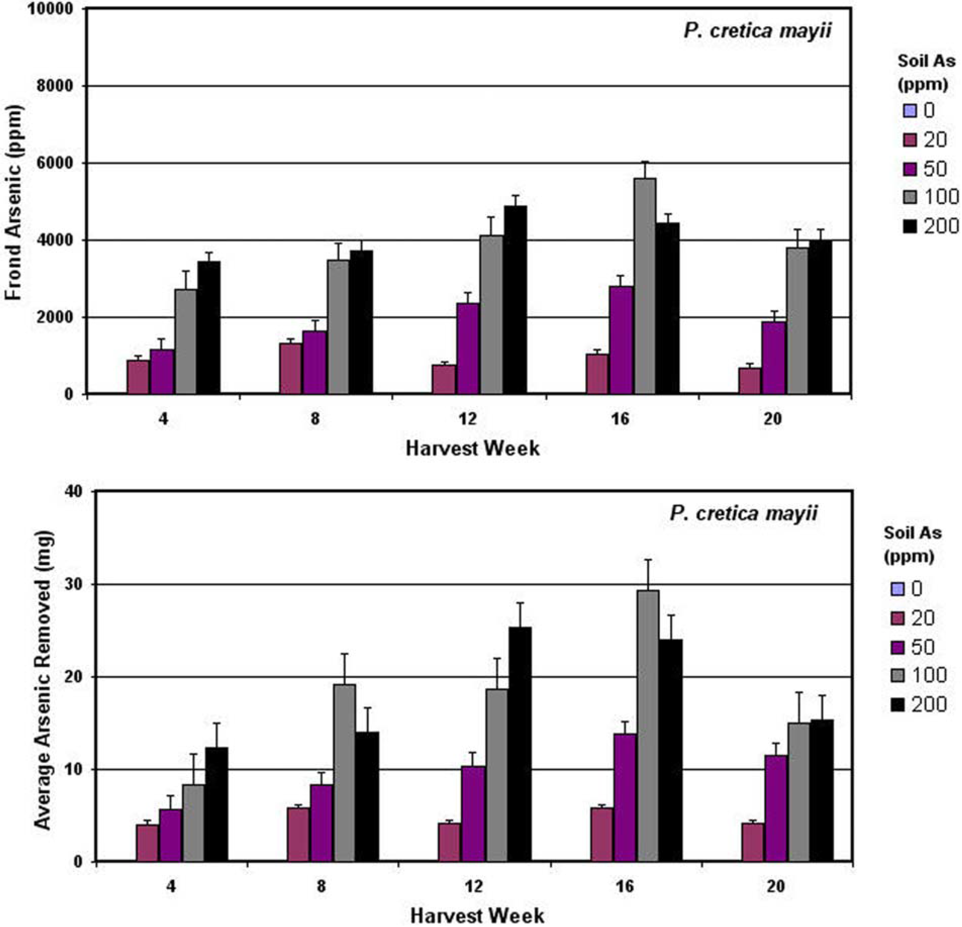
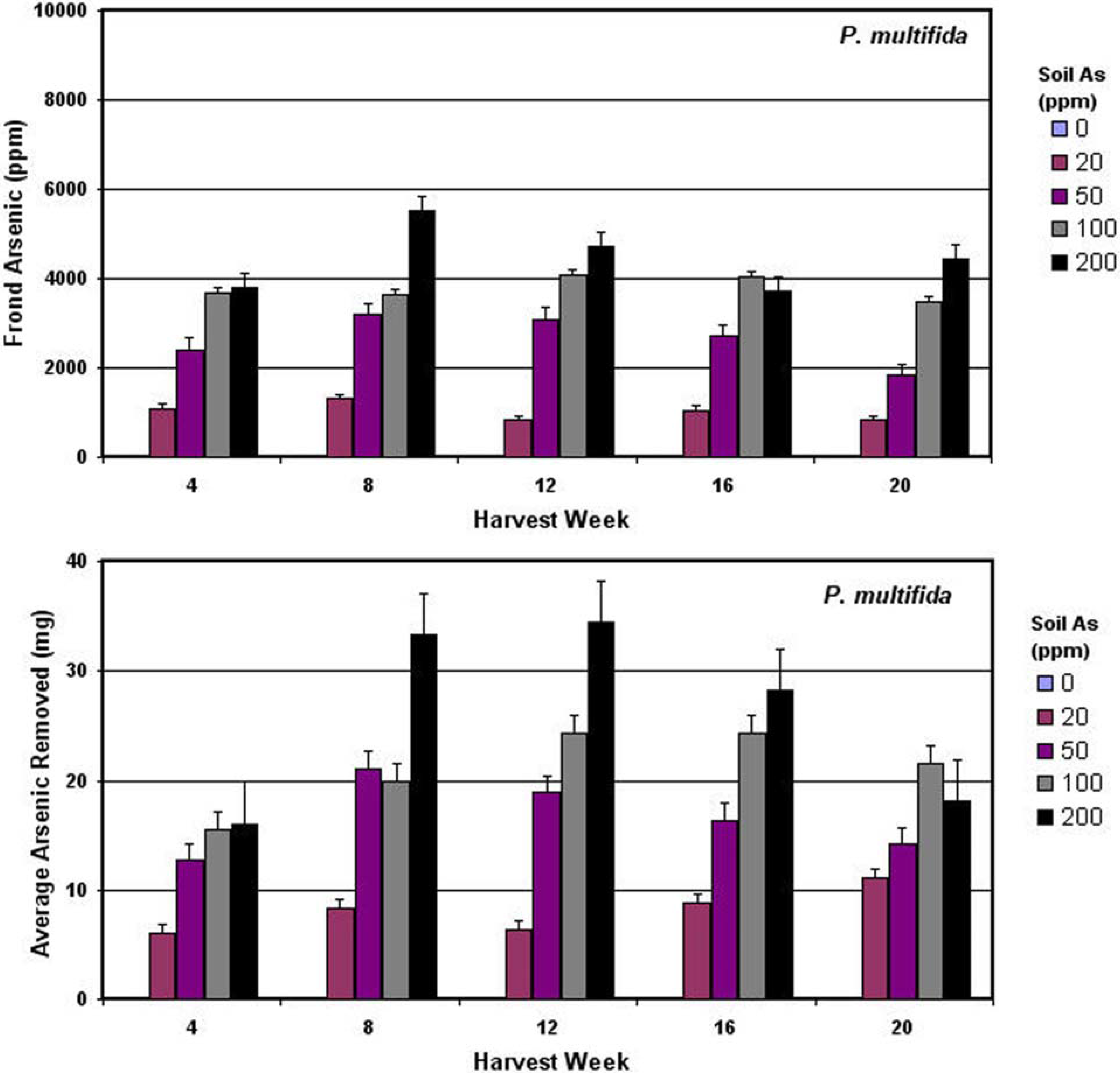
4.1. Plant Growth and Arsenic Uptake

Plant growth in soils contaminated with arsenic is generally inhibited and the effects range from depressed biomass production to extreme toxicity [71]. The Nephrolepis exaltata control fern showed moderate to severe symptoms of phytotoxicity, including chlorosis, diminished growth, leaf necrosis and plant death and these symptoms increased with the soil arsenic concentration and were evident early in the study at eight weeks (see Figure 4). The Pteris ferns also showed a pattern of decreased biomass as arsenic concentrations increased but did not display the same severe symptoms of phytotoxicity. In all ferns, there was a general inverse relationship between the soil arsenic concentration and the plant biomass at harvest. See Figure 5. Table 1, Table 2 and Table 3 show the results of the chemical analysis for arsenic for each of the three fern species over the entire study period. The tables include the Standard Error (SE) of the measurement as well as the bioconcentration factor (Plant As/ Soil As).
Figure 4. Soil arsenic concentration and plant biomass. Nephrolepis exaltata ferns at 8 weeks in soil/arsenic concentrations of (from left to right) 0, 20, 50, 100 and 200 ppm showing the general effects of increasing soil arsenic on plant growth.
Remotesensing 01 00644 g004
Figure 5. Arsenic concentration vs dryweight. The general relationships between arsenic and plant biomass for the non-accumulating control fern, Nephrolepis exaltata and for the two hyperaccumulating Pteris species. Even though the different species react differently, eventually arsenic is a stressor for all the ferns.
Remotesensing 01 00644 g005
Both Pteris ferns displayed significant uptake of arsenic at the first 4-week harvest and consistently throughout the study. In the 200-ppm soil concentration, the control fern Nephrolepis exaltata showed significant concentrations of frond arsenic beginning at the 8-week harvest and through the rest of the study. However, as the Nephrolepis exaltata fern was generally displaying symptoms of phytotoxicity at the 200 ppm soil concentration, the plant arsenic concentrations are probably due to processes and effects other than uptake alone. Figure 6, Figure 7 and Figure 8 show the arsenic concentration and total arsenic removed for each fern species.
Figure 6. Arsenic uptake summary for Nephrolepis exaltata. Arsenic concentration and content in the control fern Nephrolepis exaltata. One of the surprising results was the consistently high frond arsenic concentrations of Nephrolepis exaltata ferns grown in the 200 ppm arsenic/soil concentration. Whiskers show the standard error. Table 1 lists uptake values by week and soil concentration.
Remotesensing 01 00644 g006
Table 1. Summary Results for Arsenic Uptake in Nephrolepis exaltata. SE is the standard error. Soil As lists predicted concentration and actual concentration in parentheses.
Remotesensing 01 00644 i001
Figure 7. Arsenic Uptake Summary for Pteris cretica mayii. Arsenic concentration and content in the arsenic-hyperaccumulating fern Pteris cretica mayii. Peak concentration and content were observed after 16 weeks and, in several cases, Pteris cretica mayii seemed to accumulate more arsenic from the 100 ppm concentration than the 200 ppm concentration. Table 2 lists uptake values by week and soil concentration.
Remotesensing 01 00644 g007
Table 2. Summary Results for arsenic uptake in Pteris cretica mayii. SE is the standard error. Soil As lists predicted concentration and actual concentration in parentheses.
Remotesensing 01 00644 i002
Figure 8. Arsenic Uptake Summary for Pteris multifida. Arsenic concentration and content in the arsenic-hyperaccumulating fern Pteris multifida. Peak concentration and content were observed between eight and 12 weeks and, like, Pteris cretica mayii accumulated more arsenic from the 100 ppm concentration than from the 200 ppm concentration in some cases. Table 3 lists uptake values by week and soil concentration.
Remotesensing 01 00644 g008
Table 3. Summary Results for arsenic uptake in Pteris multifida. SE is the standard error. Soil As lists predicted concentration and actual concentration in parentheses.
Remotesensing 01 00644 i003
The Pteris ferns are known to concentrate arsenic in the fronds and the harvested frond arsenic concentrations generally correlated with the soil arsenic concentration for both Pteris multifida (r2 = 0.55) and Pteris cretica mayii (r2 = 0.57). There were some notable exceptions. Pteris cretica mayii, at the 8-week and 16-week harvests, and the Pteris multifida at the 16- and 20-week harvests, both show that either arsenic concentration or total arsenic was higher at the 100 ppm soil level than the 200 ppm soils, suggesting that there may be an upper boundary for soil arsenic concentrations and conditions between 100 ppm and 200 ppm and that there are species-specific differences in uptake rate and tolerance between Pteris species. On the final fern harvest at 20 weeks, the roots of the ferns were also collected and tested for arsenic concentration using the same methods as the fronds. Results showed that Nephrolepis exaltata, Pteris cretica mayii and Pteris multifida had root arsenic levels of 154 ppm, 701 ppm and 776 ppm respectively. The root/frond distribution of arsenic in the Pteris species is consistent with previously published results [3,6,72]. One of the working definitions of a hyperaccumulating plant is the ability to rapidly trans-locate a metal or metalloid from the roots to the above ground biomass.

4.2. Summary of Greenhouse Results

Although previously reported by Wang et al. and Wei and Chen [4,6] this study reconfirms that Pteris cretica mayii and Pteris multifida are arsenic hyperaccumulators. Both Pteris ferns achieved frond arsenic concentrations in excess of 5,000 ppm with no visual phytotoxic effects, although decreased biomass was observed at the 200 ppm soil arsenic level. The Pteris multifida ferns removed more arsenic than the Pteris cretica mayii ferns. The maximum level of frond arsenic concentration was achieved at eight weeks for Pteris multifida and at 16 weeks for Pteris cretica mayii suggesting individual species differences in arsenic uptake. Also, at several harvests, both species showed that the maximum concentration of frond arsenic and/or the maximum total arsenic was higher in the 100 ppm soil arsenic category than in the 200 ppm soil arsenic category, suggesting that there may be a upper limit for optimal arsenic hyperaccumulation for both species in the 100 ppm to 200 ppm soil arsenic concentration range. Even though there was significant uptake of arsenic by both Pteris ferns, they still were negatively affected by arsenic uptake and there was a general negative relationship between fern biomass (dry weight) and frond arsenic concentration.
Separate test for significance were conducted for the overall data set and for between species differences. In the overall data set, dryweight was signficant with soil arsenic and harvet week (p < 0.01) but not signficant with the arsenic uptake level (frond_arsenic) even at the p < 0.05 level. Frond arsenic was signficant in the overall data set with soil arsenic, species, and dryweight, (p < 0.01), but not with the harvest week. In the individual species data sets, dryweight was significant with soil arsenic only (p < 0.01), for all three species but was not signficant with any other variable for any species. For the indivudal species, frond arsenic was significant with soil_arsenic for all three species but not significant with harvest week or dry weight for any of the three species at the 95% or 99% confidence interval.
The control fern Nephrolepis exaltata displayed symptoms of stress and phytotoxicity in soil arsenic levels of 100 ppm or greater throughout the 20-week study with the level of severity directly related to the level of soil arsenic. Significant concentrations of arsenic were detected in the fronds of Nephrolepis exaltata growing in the 200 ppm soil arsenic concentration but with decreased biomass and with extreme phytotoxic effects. There was a significant inverse relationship between frond arsenic and biomass yield in the highest two soil arsenic concentrations (R2 = 0.48, p = 0.004). One important result for Nephrolepis exaltata was the frond arsenic concentrations at the 200 ppm soil arsenic level. At eight weeks and to the end of the study Nephrolepis exaltata had arsenic concentrations in excess of 4,000 ppm. It is important to note that the biomass yields of these ferns at this level were very low as they were near biological death. It is likely that the high arsenic concentrations were not related to an uptake process as in the Pteris ferns but rather other processes such as the fronds coming in direct contact with the soil due to osmotic stress and loss of turgor pressure [73].

4.3. Spectral Analysis Results

As an initial data mining step, the spectral values for each band were correlated against the known arsenic concentration and content for each plant. Figure 9 shows the results of this analysis for all three fern species. Although none of the correlation coefficients show a strong relationship, it is still evident that there is a pattern between plant arsenic and average spectral reflectance/wavelength that is likely related to basic photosynthetic processes. Several key peaks and valleys in this spectral range are located in areas of known plant phenomena.
The fern that was most efficient at arsenic uptake, Pteris multifida, shows the least amount of spectral variation and Nephrolepis exaltata, the non-accumulating fern, shows the greatest amount of spectral variation. Each of the ferns shows a negative correlation in the area of 530 nm (green reflectance peak) and a positive correlation at 680 nm (red light absorption). Other spectral areas of potential interest include a trough at 750 nm, commonly referred to as the “Red Edge” and related to plant stress. Shoulders near 980 nm and 1,180 nm are likely related to leaf or atmospheric water. Peaks near 1,460 nm and 1,950 nm probably also relate to atmospheric water vapor absorption and the trough at 1,685 nm could potentially be related to nitrogen or proteins containing nitrogen.
A second basic data visualization technique is shown in Figure 10 that displays the extreme arsenic exposure over time and the resulting spectra. The average spectra of four replicates for each species is displayed at 4 weeks in the 0 ppm soil arsenic, at 12 weeks in 50 ppm soil arsenic and at 20 weeks in 200 ppm soil arsenic. These three collections of spectra generally show the entire range of change effects that have occurred with arsenic exposure. Distinct patterns are evident in all three fern species.
These include changes in the green peak around 560 nm, changes in the red absorption trough at 680 nm and loss of the infrared shoulder around 750 nm. Other potential diagnostic features include peaks at 1,120 nm, 1,310 nm, 1,685 nm, 1,860 nm, 2,020 nm and 2,230 nm and absorption features at 1,150 nm, 1,200 nm, 1,460 nm, 1,685 nm, 1,940 nm and 2,170 nm.
PLS and SLR techniques were used to develop models of arsenic uptake in plants from the raw reflectance, and the first and second derivative data sets. The different models developed for the Reflectance, first and second derivative data are shown in Figure 3. The first derivative models for both Pteris ferns showed the best R2 and RMSE results and are listed in Table 4. It is of note that different sets of band combinations were selected for each fern and indicate that there is probably a species-specific type relationship as was also suggested in the basic uptake results.
It is likely that leaf structure and bi-directional reflectance may play an important role in band selection. Pteris cretica mayii has a broader, flatter leaf structure and for this fern, the band selection in the green (band 555), red (bands 631, 687), red-edge (band 749), near-infrared (band 998) and short-wave infrared (bands 1448, 1644 and 2184) parts of the spectrum occur in regions that could be reasonably expected from the basic data mining techniques shown in Figure 10 and Figure 11.
Figure 9. Wavelength - arsenic correlations. The first data visualization investigates the correlation between the average spectral reflectance and arsenic concentration and content, thus showing the areas of the spectrum that might yield information about the levels of arsenic in the plant.
Remotesensing 01 00644 g009
Figure 10. Spectral changes over time. A second data visualization technique plots the extremes of spectral variations of all three fern species; 0 ppm arsenic at 4 weeks, 50 ppm arsenic at 12 weeks and 200 ppm arsenic at 20 weeks. Distinct changes are evident.
Remotesensing 01 00644 g010
Pteris multifida, with a long and thin leaf structure (see Figure 2) and a more textured canopy reflectance surface also selected bands in the green (band 543) and the red-edge region (band 956) but nothing in the photosynthetic red region. Similar to Pteris cretica mayii, one band was selected in the near-infrared (band 956) and the rest in the short-wave infrared (bands 1174, 1888, 2140 and 2331).
In Pteris cretica mayii, it is clear that some interaction with the photosynthetic process is important to the presence and uptake of arsenic while this is totally absent from Pteris multifida. Both ferns showed the importance of both a green band and the red-edge and this is consistent with previous worked demonstrated by Reusen et al. and Cleavers et al. [28]. Bands at 1448, 2140 and 2331 likely relate to lignin.
Table 4. Linear Models for Predicting Arsenic Concentration from Spectral Data.
Remotesensing 01 00644 i004

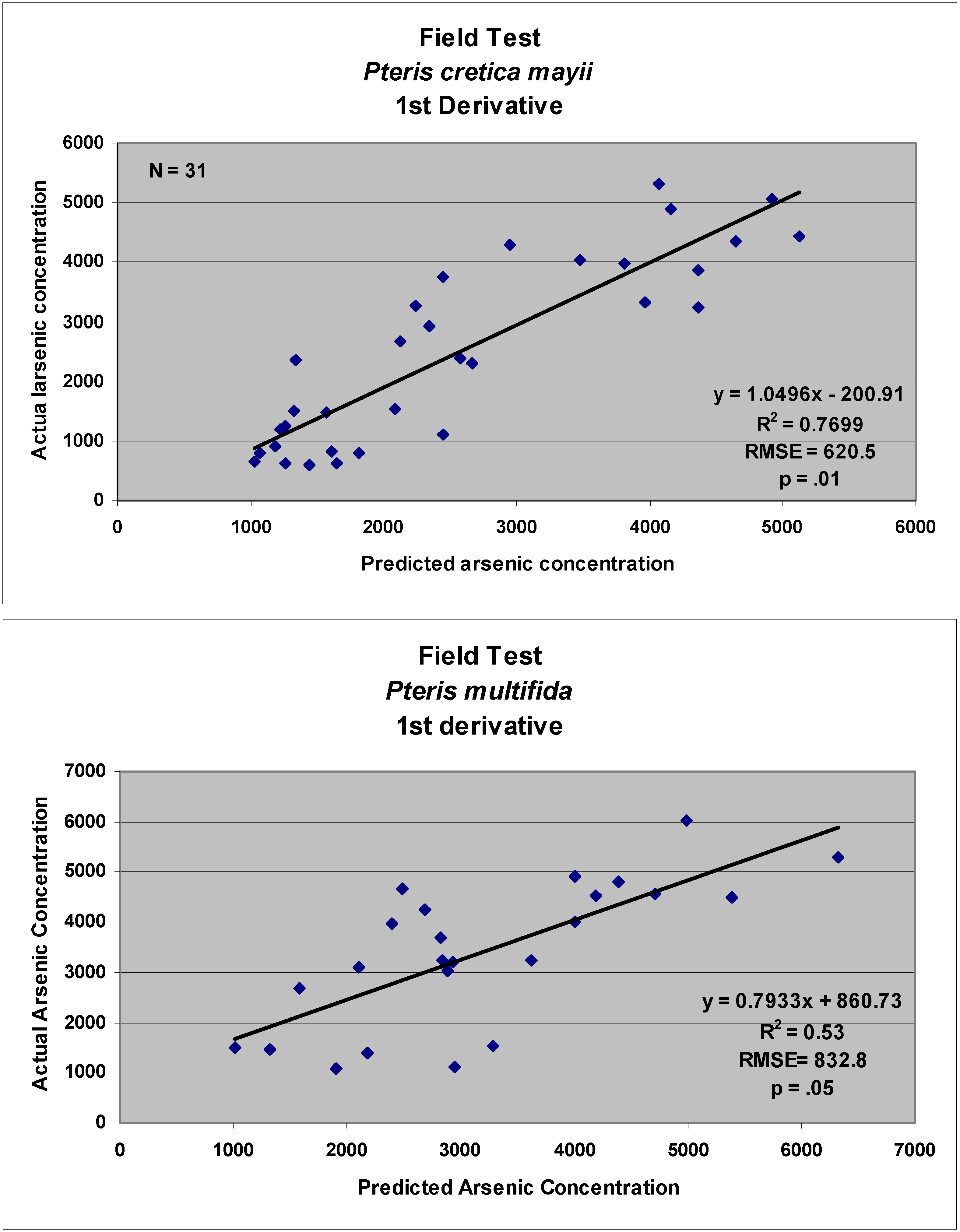
4.4. Testing Spectral-Arsenic Prediction Models

A field test data set was utilized to test the arsenic prediction models and consisted of both field and laboratory spectral collections not used in the original analysis. The spectra from these ferns were input into spreadsheets and processed into reflectance and the first and second derivatives. Data from the first and second derivatives were then used to plug into the previously developed models and to test their predictive potential. Reasonable models and accuracies were achieved with the first derivative data as shown in Figure 12.
Figure 12. Results of testing the arsenic prediction models on field data.
Remotesensing 01 00644 g011

5. Summary and Discussion

The significant outcomes of this study are results from both the greenhouse growth chamber phase and the spectral modeling. The results of the greenhouse data confirm the fact that ferns Pteris multifida and Pteris cretica mayii are, in fact, arsenic hyperaccumulators. Average concentrations of frond arsenic were nearly all above 4,000 ppm for both ferns after 12 weeks in the 100 ppm and200 ppm levels of soil arsenic. Pteris multifida was slightly more efficient at arsenic extraction than Pteris cretica mayii with average frond arsenic concentrations of 2,976 ppm and 2,773 ppm respectively (the average of the non-zero values in Table 2 and Table 3). Pteris multifida was more tolerant of high arsenic concentrations than was Pteris cretica mayii with average biomass yields of 6.5 g and 5.2 g respectively.
The control fern Nephrolepis exaltata displayed symptoms of stress and phytotoxicity early and throughout the 20-week study with the level of severity directly related to the level of soil arsenic. There was a significant inverse relationship between frond arsenic and biomass yield in the highest two soil arsenic concentrations (R2 = 0.48, p = 0.004). One important result for Nephrolepis exaltata was the frond arsenic concentrations at the 200 ppm soil arsenic level. At eight weeks and to the end of the study Nephrolepis exaltata had arsenic concentrations in excess of 4,000 ppm. It is important to note that the biomass yields of these ferns at this level were very low as they were near biological death. It is likely that the high arsenic concentrations were not related to an uptake process as in the Pteris ferns but rather other processes such as the fronds coming in direct contact with the soil due to osmotic stress and loss of turgor pressure [73].
One of the unique aspects of this experiment was that the soil arsenic was prepared so as to be highly bio-available to the ferns and both of the Pteris ferns had significant uptake of arsenic by the first harvest at four weeks. Pteris cretica mayii continued to show increases in arsenic uptake through harvest week 16 and then a slight decrease at harvest week 20. This is probably due, at least in part, to environmental conditions as this part of the study extended into October and both day and night ambient temperatures were falling. An interesting point is that Pteris cretica mayii displayed its highest level of frond arsenic concentration and its highest level of phyto-extraction at harvest week 16 and from the 100 ppm arsenic soils, not the 200 ppm arsenic soils. Pteris multifida had its highest concentration of frond arsenic at harvest week 8 and its highest level of phyto-extraction at harvest week 12. This all suggests that there are species-specific differences in the uptake profile of Pteris ferns and that specific phytoremediation applications might be developed for different ferns of the Pteris genus.
An obvious next step would be another greenhouse uptake experiment, perhaps with Pteris ferns that are native to a more temperate climate, in a variety of soil characteristics and with a completely randomized statistical design. A full climate-controlled greenhouse facility would also be desirable.
Of the three forms of spectral data evaluated, reflectance, the first derivative and the second derivative, the first derivative was the best for developing a statistical model. The reflectance data are so highly correlated that it becomes very difficult, if not impossible, to find enough components to build a robust and significant model that does not violate the collinearity condition of regression. The second derivative was very noisy and in spite of several different spectral processing software applications, is harder to calculate in reality than originally assumed. The key is in the smoothing algorithms that are used in spectral graph processing. Most of the literature in reflectance spectroscopy and imaging spectroscopy suggests employing a Savitsky–Golay smoothing algorithm that performs a local polynomial regression to determine the smoothed value for each point and offers the advantage of preserving spectral features of the distribution such as subtle absorption features, key edges and relative maxima and minima which are often destroyed by other smoothing techniques (Savitsky and Golay 1964) [74].
The development of the linear models of arsenic concentration was one of the primary goals of the study, and the results of the model development between the reflectance characteristics and the level of frond arsenic concentration are significant because of the potential to develop a non-contact monitoring tool for phytoremediation and in the larger context of “bio-reporting”, the use of plants to report back important information about landscape conditions. The ability to predict soil and geologic conditions based on vegetation spectra was first developed and explored as a form of biogeophysical mineral exploration by Milton et al. [7] and with continuing development and deployment of hyperspectral systems, this concept could be advanced to new capabilities.
One of the interesting results in the development of the spectral models of arsenic concentration was the completely different set of wavelengths for each Pteris species that proved to be optimal for prediction. The Pteris cretica models tended to use bands in the 450–700 nm range, where photosynthetic absorption and reflectance are very pronounced and known to relate to plant physiology. The Pteris multifida models mostly used bands in the infrared areas well beyond the range of photosynthetic absorption. One possibility is that the bands in the near and short wave infrared regions are related to leaf chemistry and specific chemical absorptions. For example, Kokaly and Clark demonstrated that there were narrow infrared band centers that were related to absorptions of specific chemical compounds [75]. Pteris models bands at 1,658, 2,088 and 2,324 nm have been shown to relate to cellulose, nitrogen and lignin respectively.

References

  1. Ma, L.Q.; Komar, K.M.; Tu, C.; Zhang, W.; Cai, Y. A fern that hyperaccumulates arsenic. Nature 2001, 409, 579. [Google Scholar] [CrossRef] [PubMed]
  2. Zhao, F.J.; Dunham, S.J.; McGrath, S.P. Arsenic hyperaccumulation by different fern species. New Phytol. 2002, 156, 27–31. [Google Scholar] [CrossRef]
  3. Srivastava, M.; Ma, L.Q.; Gonzaga-Santos, J.A. Three new arsenic hyperaccumulating ferns. Sci. Total Envion. 2006, 364, 24–31. [Google Scholar] [CrossRef] [PubMed]
  4. Wang, H.B.; Wong, M.H.; Lan, C.Y.; Baker, A.J.M.; Qin, Y.R.; Shu, W.S.; Chen, G.Z.; Ye, Z.H. Uptake and accumulation of arsenic by 11 Pteris taxa from southern china. Environ. Pollut. 2006, 20, 1–9. [Google Scholar]
  5. Blaylock, M.J.; Elless, M.P.; Bray, C.A.; Teeter, C.L. Phytoremediation of arsenic contaminated soil in Spring Valley FUDS of Washington, D.C.; Edenspace Systems: Dulles, VA, USA, 2005. [Google Scholar]
  6. Wei, C.Y.; Chen, T.B. Arsenic accumulation by two brake ferns growing on an arsenic mine and their potential in phytoremediation. Chemosphere 2006, 63, 1048–1053. [Google Scholar] [CrossRef] [PubMed]
  7. Milton, N.M.; Collins, W.; Chang, S.H. Confirmation of Airborne biogeophysical mineral exploration technique using laboratory methods. Econ. Geol. 1983, 78, 723–736. [Google Scholar]
  8. Milton, N.M.; Ager, C.M.; Eisworth, B.A.; Powers, M.S. Arsenic and selenium induced changes in spectral reflectance and morphology of soybean plants. Remote Sens. Environ. 1989, 30, 263–269. [Google Scholar] [CrossRef]
  9. Rock, B.N.; Hoshizake, T.; Miller, J.R. Comparison of in situ and airborne spectral measurements of the blue shift with forest decline. Remote Sens. Environ. 1988, 24, 109–127. [Google Scholar] [CrossRef]
  10. Milton, N.M.; Eisworth, B.A.; Ager, C.M. Effect of phosphorous deficiency on spectral reflectance and morphology of soybean plants. Remote Sens. Environ. 1991, 36, 121–127. [Google Scholar] [CrossRef]
  11. Rood, J.W. Jr. Modern Chromatics with Applications to Art and Industry; D. Appleton & Company: New York, NY, USA, 1879. [Google Scholar]
  12. Murtha, P.A. Vegetation. In The Manual of Photographic Interpretation; Phillipson, W.R., Ed.; American Society for Photogrammetry and Remote Sensing: Bethesda, MD, USA, 1997. [Google Scholar]
  13. Schull, C.A. A spectrophotometric study of reflection of light from leaf surfaces. Bot. Gaz. 1929, 87, 583–607. [Google Scholar] [CrossRef]
  14. McNicholas, H.J. The visible and ultraviolet absorption spectra of carotin and xanthophyll and the changes accompanying oxidation. J. Res. Natl. Bur. Stand. 1931, 7, 171–193. [Google Scholar] [CrossRef]
  15. Gates, D.M.; Keegan, H.J.; Schleter, J.C.; Weidner, V.R. Spectral properties of plants. Appl. Opt. 1965, 4, 11–20. [Google Scholar] [CrossRef]
  16. Guyot, G.; Baret, F.; Jacquemoud, S. Modeled analysis of the biophysical nature of spectral shifts and comparison with information content of broad bands. Remote Sens. Environ. 1992, 41, 145–165. [Google Scholar]
  17. Ray, T.W.; Muray, B.C.; Chehbouni, A.; Njoku, E. The Red edge in arid region vegetation: 340 – 1060 nm spectra. In Summaries of the Fourth Annual JPL Airborne Geoscience Workshop; JPL Publication 93–26; Jet Propulsion Laboratory: Pasadena, CA, USA, 1993; pp. 149–152. [Google Scholar]
  18. Horler, D.N.H.; Dockray, M.; Barber, J.; Barringer, A.R. Red edge measurements for remote sensing plant chlorophyll content. Adv. Space Res. 1983, 3, 273–277. [Google Scholar] [CrossRef]
  19. Baret, F.I.; Champion, G.; Guyot, G.; Podaire, A. Monitoring wheat canopies with a high spectral resolution radiometer. Remote Sens. Environ. 1987, 2, 367–378. [Google Scholar] [CrossRef]
  20. Collins, W.; Raines, G.L.; Canney, F.C. Airborne spectroradiometer discrimination of vegetation anomalies over sulfide mineralization – a remote sensing technique. In Abstracts with programmes, Geological Society of America Annual Meeting, Seattle, Washington, DC, USA, 7 – 9 November 1977; pp. 932–933.
  21. Horler, D.N.H.; Barber, J.; Barringer, A.R. Effects of heavy metals on the absorbance and reflectance spectra of plants. Int. J. Remote Sens. 1980, 1, 121–136. [Google Scholar] [CrossRef]
  22. Schwaller, M.R.; Tkach, S.J. Premature leaf senescence: remote sensing detection and utility for geobotanical prospecting. Econ. Geol. 1985, 80, 250–255. [Google Scholar] [CrossRef]
  23. Anderson, J.E.; Robbins, E.I. Spectral reflectance and detection of iron–oxide precipitates associated with acidic mine drainage. Photogramm. Eng. Remote Sens. 1998, 64, 1201–1208. [Google Scholar]
  24. Swayze, G.A.; Smith, K.S.; Clark, R.N.; Sutley, S.J.; Pearson, R.M.; Vance, J.S.; Hageman, P.L.; Briggs, P.H.; Meier, A.L.; Singleton, M.J.; Roth, S. Using imaging spectroscopy to map acidic mine waste. Environ. Sci. Technol. 2000, 34, 47–54. [Google Scholar] [CrossRef]
  25. Kooistra, L.J.; Wehrens, R.; Leuven, E.W.; Buydens, L.M.C. Possibilities of visible–near–infrared spectroscopy for the assessment of soil contamination in river floodplains. Anal. Chim. Acta 2001, 446, 97–105. [Google Scholar] [CrossRef]
  26. Kooistra, L.J.; Wanders, G.F.; Epema, R.S.; Leuven, E.W.; Wehrens, R.; Buydens, L.M.C. The potential of field spectroscopy for the assessment of sediment properties in river floodplains. Anal. Chem. Acta 2003, 484, 189–200. [Google Scholar] [CrossRef]
  27. Kooistra, L.; Salas, E.A.L.; Clevers, J.G.P.; Wehrens, R.; Luevens, R.S.E.W.; Nienhuis, P.H.; Buydens, L.M.C. Exploring field vegetation reflectance as an indicator of soil contamination in river foodplains. Environ. Pollut. 2004, 127, 281–290. [Google Scholar] [CrossRef]
  28. Clevers, J.; Kooistra, L.; Salas, E.A.L. Study of heavy metal contamination in river floodplains using the red-edge position in spectroscopic data. Int. J. Remote Sens. 2004, 25, 1–13. [Google Scholar] [CrossRef]
  29. Rosso, P.H.; Pushnik, J.C.; Lay, M.; Ustin, S.L. Reflectance properties and physiological responses of salicornia virginica to heavy metal and petroleum contamination. Environ. Pollut. 2005, 137, 241–252. [Google Scholar] [CrossRef] [PubMed]
  30. Schuerger, A.C.; Capelle, G.A.; Di Benedetto, J.A.; Maoc, C.; Thaid, C.N.; Evans, M.D.; Richards, J.T.; Blank, T.A.; Stryjewski, E.C. Comparison of two hyperspectral imaging and two laser-induced fluorescence instruments for the detection of zinc stress and chlorophyll concentration in Bahia Grass (Paspalum notatum Flugge.). Remote Sens. Environ. 2003, 84, 572–588. [Google Scholar] [CrossRef]
  31. Sridhar, M.B.B.; Han, F.X.; Diehl, S.V.; Monts, D.L.; Su, Y. Monitoring the effects of arsenic and chromium accumulation in chinese brake fern (Pteris vittata). Int. J. Remote Sens. 2007, 28, 1055–1067. [Google Scholar] [CrossRef]
  32. CERCLA. Comprehensive environmental response, Compensation, and Liability Act (commonly known as Superfund). Public Law 96–510, 42 U.S.C. §§ 9601et seq. 1980. [Google Scholar]
  33. Gorby, M.S. Arsenic in human medicine. In Arsenic in the Environment; Nriagu, J.O., Ed.; Part II: Human Health and Ecosystem; John Wiley & Sons: New York, USA, 1994. [Google Scholar]
  34. Azcue, J.M.; Nriague, J.O. Arsenic: Historical perspectives. In Arsenic in the Environment; Nriagu, J.O., Ed.; Part I: Cycling and Characterization; John Wiley & Sons: New York, NY, USA, 1994. [Google Scholar]
  35. NRC (National Research Council). Arsenic in Drinking Water; National Academy of Sciences: Washington, DC, USA, 1999. [Google Scholar]
  36. Focazio, M.J.; Welch, A.H.; Watkins, S.A.; Helsel, D.R.; Horn, M.A. A retrospective analysis on the occurrence of arsenic in ground–water resources of the United States and limitations in drinking–water–supply characterizations. In U.S. geological survey water–resources investigations report 99–4279; U.S. Geological Survey: Reston, VA, USA, 1999. [Google Scholar]
  37. Karim, M.M. Arsenic exposure modeling and risk assessment in Bangladesh using geographic information system. In Proceedings of The Second International Health Geographics Conference, Washington, DC, USA, 17 – 19 March 2000; pp. 35–42.
  38. Duble, R.L.; Thomas, J.C.; Brown, K.W. Arsenic pollution from underdrainage and runoff from golf greens. Agron. J. 1978, 70, 71–74. [Google Scholar] [CrossRef]
  39. A citizen’s guide to bioremediation; EPA–F42–01–001; Office of Solid Waste and Emergency Response: Washington, DC, USA, 2001.
  40. Boyajian, G.E.; Devedjian, D.L. Phytoremediation: it grows on you. Soil and Groundwater Cleanup 1997, 22–26. [Google Scholar]
  41. Peart, V. Indoor Air Quality in Florida: Houseplants to Fight Pollution; Publication FCS 3208, Department of Family, Youth and Community Services, Florida Cooperative Extension Service, Institute of Food and Agricultural Sciences; University of Florida: Gainesville, FL, USA, 1993. [Google Scholar]
  42. Bondada, B.R.; Ma, L.Q. Tolerance of heavy metals in vascular plants: arsenic hyperaccumulation by chinese brake fern (Pteris vittata L.). In Pteridology in the New Millennium; Chandra, S., Srivastava, M., Eds.; Kluwer Academic: Dordrecht, The Netherlands, 2003; pp. 397–420. [Google Scholar]
  43. Blaylock, M.J. The controlled growth of arsenic hyperaccumulating ferns to support EPA spectral imaging studies; Edenspace Systems Corporation: Dulles, VA, USA, 2005. [Google Scholar]
  44. Method 3050b, Acid digestion of sediments, sludges, and soils; U.S. Environmental Protection Agency: Washington, DC, USA, 2004.
  45. FieldSpec Users Guide; Analytical Spectral Devices: Boulder, CO, USA, 1997.
  46. Hansen, P.M.; Jorgenson, J.R.; Thomsen, A. Predicting grain yield and protein content in winter wheat and spring barley using repeated canopy reflectance measurements and partial least squares regression. J. Agric. Sci. 2002, 139, 307–318. [Google Scholar] [CrossRef]
  47. Schmidtlein, S. Imaging spectroscopy as a tool for mapping ellenberg indicator values. J. Appl. Ecol. 2005, 42, 966–974. [Google Scholar] [CrossRef]
  48. Wold, H. Estimation of principal components and related models by iterative least squares. In Multivariate Analysis; Krishnaiah, P.R., Ed.; Academic Press: New York, NY, USA, 1966; pp. 391–420. [Google Scholar]
  49. Abdi, H. Partial least squares regression (PLS-regression). In Encyclopedia for Research Methods for the Social Science; Lewis-Beck, M., Futing, B.T., Eds.; Sage Publishing: Thousand Oaks, CA, USA, 2003; pp. 792–795. [Google Scholar]
  50. Höskuldsson, A. PLS regression methods. J. Chemometr. 1988, 2, 211–228. [Google Scholar] [CrossRef]
  51. Rosipal, R.; Krämer, N. Overview and recent advances in partial least squares. In Subspace, Latent Structure and Feature Selection Techniques; Saunders, C., Grobelnik, M., Gunn, S., Shawe-Taylor, J., Eds.; Springer: New York, NY, USA, 2006; pp. 34–51. [Google Scholar]
  52. Wold, H. Path with Latent Variables: The NIPALS Approach. In Quantitative Sociology: International Perspectives on Mathematical and Statistical Model Building; Balock, H.M., Ed.; Academic Press: New York, NY, USA, 1975; pp. 307–357. [Google Scholar]
  53. Wold, H. Partial Least Squares. In Encyclopedia of Statistical Sciences; Kotz, S., Johnson, N.L., Eds.; Wiley: New York, NY, USA, 1985; Volume 6, pp. 581–591. [Google Scholar]
  54. Wold, S.; Sjolstrom, M.; Erikson, L. PLS–regression: A basic tool of chemometrics. Chemometr. Intell. Lab. Syst. 2001, 58, 109–130. [Google Scholar] [CrossRef]
  55. Kresta, J.V.; Macgregor, J.F.; Marlin, T.E. Multivariate statistical monitoring of process operating performance. Can. J. Chem. Eng. 1991, 69, 35–47. [Google Scholar] [CrossRef]
  56. MacGregor, J.F.; Jaeckle, C.; Kiparissides, C.; Koutoudi, M. Process systems engineering: process monitoring and diagnosis by multiblock PLS methods. AIChE J. 2004, 40, 826–838. [Google Scholar] [CrossRef]
  57. Nyberg, L.; Forkstam, C.; Petersson, K.M.; Cabeza, R.; Cabeza, M.; Ingvar, M. Brain imaging of human memory systems: Between–systems similarities and within–system differences. Cogn. Brain Res. 2002, 13, 281–292. [Google Scholar] [CrossRef]
  58. Habeck, C.; Krakauer, J.W.; Ghez, C.; Sackeim, H.A.; Eidelberg, D.; Stern, Y.; Moeller, J.R. A new approach to spatial covariance modeling of functional brain imaging data: ordinal trend analysis. Neural. Comput. 2005, 17, 1602–1645. [Google Scholar] [CrossRef] [PubMed]
  59. Nash, M.S.; Chaloud, D.J.; Lopez, R.D. Applications of canonical correlation and partial least squares in landscape ecology; EPA Report EPA/600/X–05/004; Environmental Sciences Division, U.S. Environmental Protection Agency: Las Vegas, NV, USA, 2005.
  60. Wold, S. PLS for multivariate linear modeling. In QSAR: Chemometric Methods in Molecular Design, Methods and Principles in Medicinal Chemistry; van de Waterbeemd, H., Ed.; Verlag Chemie: Weinheim, Germany, 1995; Volume 2, pp. 195–218. [Google Scholar]
  61. Martin, M.E.; Newman, S.D.; Aber, J.D.; Congalton, R.G. Determining forest species composition using high spectral resolution remote sensing data. Remote Sens. Environ. 1998, 65, 249–254. [Google Scholar] [CrossRef]
  62. Chen, Z.; Curran, P.J.; Hansom, J.D. Derivative reflectance spectroscopy to estimate suspendedsediment concentration. Remote Sens. Environ. 1992, 40, 67–77. [Google Scholar] [CrossRef]
  63. Demetriades-Shah, T.H.; Steven, M.D.; Clark, J.A. High resolution derivative spectra in remote sensing. Remote Sens. Environ. 1990, 33, 55–64. [Google Scholar] [CrossRef]
  64. Tsai, F.; Philpot, W. Derivative analysis of hyperspectral data. Remote Sens. Environ. 1998, 66, 41–51. [Google Scholar] [CrossRef]
  65. Wessman, C.A.; Aber, J.D.; Peterson, D.L.; Melillo, J.M. Foliar analysis using near infrared spectroscopy. Can. J. For. Res. 1988, 18, 6–11. [Google Scholar] [CrossRef]
  66. Yoder, B.J.; Pettigrew-Crosby, R.E. Predicting nitrogen and nhlorophyll nontent and concentrations from reflectance spectra (400 – 2500 nm) at leaf and canopy scales. Remote Sens. Environ. 1995, 53, 199–211. [Google Scholar] [CrossRef]
  67. Kosmas, C.S.; Curi, N.; Bryant, R.B.; Franzmeier, D.P. Characterization of iron oxide minerals by second derivative visible spectroscopy. J. Soil Sci. Soc. Amer. 1984, 48, 401–405. [Google Scholar] [CrossRef]
  68. Adams, M.L.; Philpot, W.D.; Norvell, W.A. Yellowness index: an application of spectral second derivatives to estimate chlorosis of leaves in stressed vegetation. Int. J. Remote Sens. 1999, 18, 3663–3675. [Google Scholar] [CrossRef]
  69. Chen, Z.; Elvidge, C.D.; Jansen, W.T. Description of a derivative-based high spectral-resolution (AVIRIS) green vegetation index. In Proceedings of Imaging Spectrometry of the Terrestrial Environment; SPIE: Orlando, FL, USA, 1993; pp. 43–54. [Google Scholar]
  70. Dixit, L.; Ram, S. Quantitative analysis by derivative electronic spectroscopy. Appl. Spectrosc. Rev. 1985, 21, 311–418. [Google Scholar] [CrossRef]
  71. Eisler, R. A review of arsenic hazards to plants and animals with emphasis on fishery and wildlife resources. In Arsenic in the Environment; Nriagu, J.O., Ed.; Part II: Human Health and Ecosystem Effects; John Wiley & Sons: New York, NY, USA, 1994; pp. 185–261. [Google Scholar]
  72. Bondada, B.R.; Ma, L.Q. Tolerance of heavy metals in vascular plants: arsenic hyperaccumulation by chinese brake fern (Pteris vittata L.). In Pteridology in the New Millennium; Chandra, S., Srivastava, M., Eds.; Kluwer Academic Publishers: Dordrecht, The Netherlands, 2003; pp. 397–420. [Google Scholar]
  73. Jones, H.G.; Flowers, T.L.; Jones, M.B. Plants Under Stress; Cambridge University Press: New York, NY, USA, 1989. [Google Scholar]
  74. Savitsky, A.; Golay, M.J.E. Smoothing and differentiation of data by simplified least squares procedures. Anal. Chem. 1964, 36, 1627–1639. [Google Scholar] [CrossRef]
  75. Kokaly, R.F.; Clark, R.N. Spectroscopic determination of leaf biochemistry using band-depth analysis of absorption features and stepwise multiple linear regression. Remote Sens. Environ. 1999, 67, 267–287. [Google Scholar] [CrossRef]

