Article

Derivation of Soil Line Influence on Two-Band Vegetation Indices and Vegetation Isolines

1
Department of Information Science and Technology, Aichi Prefectural University, 1522-3 Kumabari, Nagakute, Aichi 480-1198, Japan
2
Department of Natural Resources and Environmental Management, College of Tropical Agriculture and Human Resources, University of Hawaii at Manoa, 1910 East-West Road, Honolulu, HI 96822, USA
3
Department of Soil Science, University of São Paulo, Av. Pádua Dias, 11, Piracicaba, São Paulo, Brazil
4
Natural Resources Conservation Service, USDA, 355 East Hancock Avenue, Athens, GA 30601, USA
5
Department of Soil, Water and Environmental Science, University of Arizona, 1177 East Fourth Street, Tucson, AZ 85721, USA
*
Author to whom correspondence should be addressed.
Remote Sens. 2009, 1(4), 842-857; https://doi.org/10.3390/rs1040842
Submission received: 3 September 2009 / Revised: 16 October 2009 / Accepted: 27 October 2009 / Published: 3 November 2009

Abstract

:
This paper introduces derivations of soil line influences on two-band vegetation indices (VIs) and vegetation isolines in the red and near infra-red reflectance space. Soil line variations are described as changes in the soil line parameters (slope and offset) and the red reflectance of the soil surface. A general form of a VI model equation written as a ratio of two linear functions (e.g., NDVI and SAVI) was assumed. It was found that relative VI variations can be approximated by a linear combination of the three soil parameters. The derived expressions imply the possibility of estimating and correcting for soil-induced bias errors in VIs and their derived biophysical parameters, caused by the assumption of a general soil line, through the use of external data sources such as regional soil maps.

1. Introduction

Spectral vegetation indices (VIs) are a commonly used technique in satellite-based environmental monitoring in regional to global scales. Global VI products, whose history are nearly three decades, are considered one of the key parameters in various fields of study such as global climate change, drought monitoring [1], and crop yield prediction [2], and expected to be produced continuously from future satellite missions [3,4].
VIs are spectral transformations of multi-band reflectances, often involving red and near infra-red (NIR) bands, into a scalar non-dimensional variable to extract and enhance the signal contribution from green vegetation. Since an observed reflectance is a mixture of signals from various objects, influences from non-vegetated surface are not negligible. Especially, the signal contribution from canopy/soil background is known to be one major source of variations in VI values. Numerous studies have been conducted to minimize canopy/soil background influences on VI values [5,6,7,8,9,10,11]. A systematic investigation and theoretical formulation on the impact of canopy/soil background has yet to be investigated and would be a critical and meaningful contribution to operational monitoring of terrestrial vegetation with satellite VI time series [7,12,13,14,15,16]. Investigations are still needed to clarify systematic variations of VI value due to differences in soil optical properties, and that result in a methodology to adjust VI [17,18], e.g., about bias error, for site-specific canopy background influences [19].
Red and NIR reflectances of soils have been known to form a linear relationship in the reflectance space, called the “soil line” concept [15,20]. Theoretical basis of the soil line concept have been investigated and widely accepted by many researchers [7,12,13,18,20,21,22,23]. Meanwhile, due to the variability of soil line by soil type, Baret et al. [20] rejected the existence of a globally applicable soil line (a general soil line). At the same time, Baret et al. [20] concluded that the soil line concept was very robust when the soil types were separated. This fact drew our attention to the possibility of a systematic investigation of soil noise on VIs using soil line parameters.
The soil line concept has been the basis of various two-band VIs. Those VIs can be divided into two categories: (1) ratio based VIs (or angular based VIs) such as ratio VI (RVI) [24], normalized difference VI (NDVI) [25], and (2) orthogonal based VIs (or distance based VIs) such as perpendicular VI (PVI) [11], difference VI (DVI) [25], and weighted difference VI (WDVI) [26]. For all the VIs, regardless of their categories, a general soil line that represents zero vegetation pixels within a target region serves as the baseline values or offsets. Any positive deviations away from the offsets are considered contributions from green vegetation, which are then used to estimate biophysical parameters. However, due to variations of soil lines among different soil types, these baseline values also show variations [12,27,28]. As a result, errors are induced in the estimation of vegetation biophysical parameters. Since the deviation of an individual soil line from a general soil line is inevitable [12,27,28], possible variations in VI values induced by these deviations must be investigated.
Limiting our discussion to the errors induced by soil surfaces, there are two sources of influence on VI. The first one is variation of soil brightness (in absolute sense) without changing soil types. In this case, a soil line remains nearly the same. This variation is induced by soil moisture content or soil roughness while the soil line parameters are left unchanged. The second influence is variation of soil line parameters (slope and intercept) due to differences in soil type. Since these parameters together can represent soil variation in the red-NIR reflectance space, they are suitable for a systematic analysis of VI’s behavior. Another advantage of using soil line parameters is that we can avoid parameter studies about variations of soil surface, since some aspects of soil influence can be reduced into the simple expression. In this context, an analytical form of a vegetation isoline (a set of reflectance spectra from a constant canopy with different soils [29,30]) was also assumed to be subject to systematic investigations. (The details of the vegetation isoline is in subsection 2.3.) Undoubtedly, the scientific potential of such techniques has not been exhausted, and such investigations should contribute to a better understanding of VI properties and behavior.
The objective of this paper is to derive analytical expressions of soil influences on both VI and vegetation isoline as a function of the three parameters which characterize the differences in soil type, namely, (1) soil line slope, (2) NIR-intercept of soil line, and (3) red reflectance of soil. For a VI model equation, a general form of the two-band VI is assumed to cover those defined as a ratio of two linear combinations of red and NIR reflectances, such as NDVI and soil-adjusted VI (SAVI) [8]. In this paper, we first describe our framework of analysis of the soil line and vegetation isoline equations, including the model assumptions used for the derivation of these equations in Section 2. We then present the derivation of analytical expressions that describes variations of top-of-canopy reflectances induced by variations in the three soil parameters in Section 3. In Section 4, the derived analytical expressions are translated into the general VI form, which allows the propagation of soil parameter variations to VI variations. Section 5 discusses characteristics of soil influences on VIs that are found from the derived analytical equations in this study. Our conclusions are presented in Section 6.

2. Soil Line and Vegetation Isoline Equations

2.1. Soil Line Equation

A robust relationship between red and NIR reflectances from a single soil type is often characterized by a soil line equation,
R s N = a R s R + b ,
where a and b are soil line parameters, and R s N and R s R are NIR and red reflectances of a target soil, respectively. Although many studies reported general values of a and b, these two parameters depend on chemical and mineral contents, proportion of organic matter, soil moisture, and hence these are unique to individual soil type [15,19,23,31,32]. It is also known that these parameters vary with band position and band width properties of a multispectral sensor [12,33,34,35], indicating the uniqueness of these parameters to each sensor. Since the soil line parameters depend on soil type and band configuration, it is important to know possible variations of VI value against changes in the soil line parameters under an identical vegetation canopy.

2.2. Model Assumptions

In order to add canopy optical properties to the presented soil lines, the vegetation isoline equations were obtained by assuming a simple canopy model. We first assume that a portion of the target area is covered with a homogeneous vegetation canopy [36]. A parameter called fraction of green cover is defined as a fraction of the target area covered and shaded by vegetation canopies at a particular combination of illumination and viewing geometries.
We define two types of leaf area indices (LAI) in this study, local and total LAI. The local LAI is defined as an LAI within an area covered by green vegetation, whereas the total LAI is defined as a multiplication of local LAI and fraction of green cover. The local LAI is simply refereed to as “LAI” throughout this paper.
We further simplified the model so that the projection of vegetation canopy is identical to a fraction of soil obscured and shaded by the canopy. Under this simplification, the radiative transfer problem in both covered and uncovered area can be simulated independently by modeling horizontally infinite homogeneous canopy and bare soil, respectively. Thus, the reflectance from a covered area can be simulated by a turbid medium canopy model such as the SAIL model [37,38]. Reflectance contributions from each fractional area are, therefore, obtained by a weighted sum of the two independent simulations. The fraction of green cover is then used as their weights. The Lambertian surface was assumed as a background soil layer in this study.

2.3. Vegetation Isoline Equations

Based on the assumptions made in the previous subsection, reflectance at top-of-the-canopy (TOC) is approximated by a linear combination of the contributions from green-covered area and uncovered area (bare soil) with β and ( 1 β ) as their weights, where β is defined as the fraction of an area in consideration covered by vegetation at a certain illumination and viewing geometry [36]. We represent the reflectance for the green fractional area using the Cooper-Smith-Pitts model [39], also known as the adding method [40]. The other portion of reflectance ( 1 β ), which reaches to the soil without seeing the canopy layer, is then reflected back to the sensor or absorbed by the soil surface (no interaction with the canopy layer). Under these approximations, the reflectance of this system, ρ λ ( θ , ϕ , θ 0 ) , at the view angle of ( θ , ϕ ) with the sun angle of θ 0 at the wavelength of λ is then represented by the following equation [30],
ρ λ ( θ , ϕ , θ 0 ) = β ρ v λ ( θ , ϕ , θ 0 ) + β T v λ 2 ( θ , θ 0 ) R s λ 1 R v λ R s λ + ( 1 β ) R s λ
where T v λ is the geometric mean of downward T v λ ( θ 0 ) and upward T v λ ( θ ) transmittance of the canopy layer defined by
T v λ ( θ , θ 0 ) = T v λ ( θ 0 ) T v λ ( θ ) .
ρ v λ ( θ , ϕ , θ 0 ) represents the canopy reflectance with the perfect absorber as its background (or the free boundary condition), R s λ is bi-hemispherical reflectance of background, and R v λ is bi-hemispherical reflectance of vegetation canopy for the photons entering from bottom of the canopy layer and scattering out from the surface downward.
The leading two terms of right hand side (RHS) are the contributions from the green cover portion. The first term is the pure canopy reflectance representing the photons that never reached the soil surface. The second term is the contribution of photons which are reflected at least once by the soil. The last term is the contribution from the bare soil. We will omit the functional arguments in ρ λ ( θ , ϕ , θ 0 ) and ρ v λ ( θ , ϕ , θ 0 ) as ρ λ and ρ v λ for brevity. The subscripts R and N are used for λ to denote red and NIR bands, respectively.
In order to derive a vegetation isoline equation, we retain only the first-order interaction contribution of the second term of RHS in Equation (2) for each wave band,
ρ N = β ρ v N + [ β T v N 2 + ( 1 β ) ] R s N ,
ρ R = β ρ v R + [ β T v R 2 + ( 1 β ) ] R s R .
Using the soil line equation, Equation (1), with Equations (4a) and (4b), we can eliminate the soil reflectances ( R s R and R s N ) to obtain a vegetation isoline equation
ρ N = a γ ρ R + D ,
with the following definitions,
γ = β T v N 2 + ( 1 β ) β T v R 2 + ( 1 β ) ,
D = D N a γ D R ,
D N = β ρ v N + b [ β T v N 2 + ( 1 β ) ] ,
D R = β ρ v R .
The details of the derivation and explanation of the variables are provided in our previous work [30]. The denominator and numerator of γ are a weighted sum of the two-way transmittance and unity with β and ( 1 β ) as their weights. Those values are strongly related to LAI through the fraction of green cover and the canopy transmittance. Hence γ can be understood as the ratio of an area-averaged two-way transmittance of the NIR band to that of the red band. D denotes the NIR-intercept of the isoline which consists of D N and D R that are functions of only NIR and red band, respectively.
Variations of vegetation indices are caused by the discrepancy between the vegetation isolines and index isolines [8,10,41,42]. Therefore, we first need to investigate the variation pattern of vegetation isolines caused by the variation of soil line parameters.

3. Soil Line Influence on Vegetation Isoline

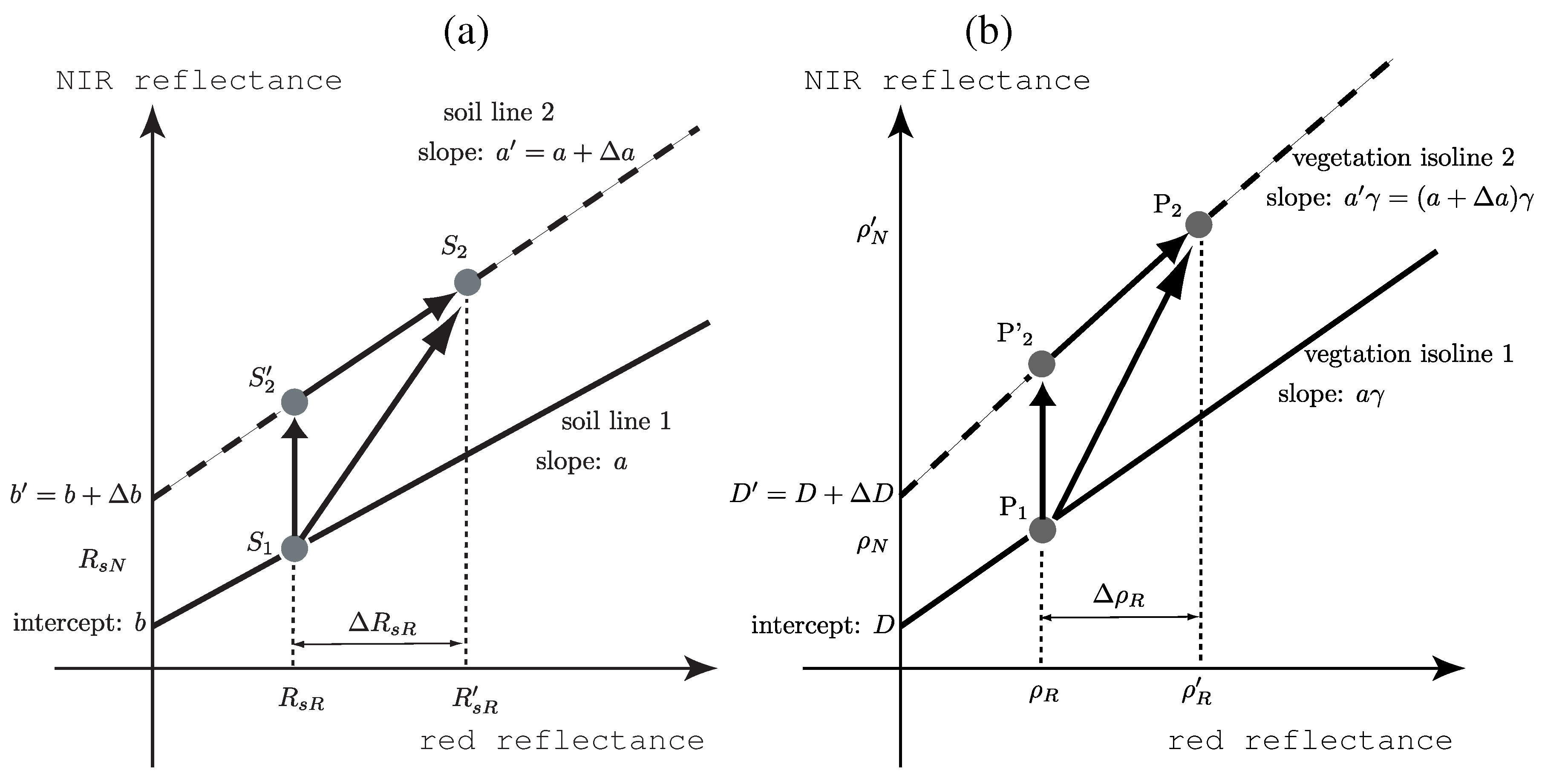
3.1. Representation of Soil Line Variation

Variations of TOC reflectances induced by the differences of soil line are derived in this subsection. The soil line parameters (a and b) and the soil reflectance of the red band ( R s R ) are used to represent such variations during the derivation. The specific goal is to write Δ ρ N and Δ ρ R as a function of Δ a , Δ b and Δ R s R . Note that the NIR reflectance of soil is a dependent variable in this derivation (see Equation (1)).
We first assume that the original soil line (or a general soil line) was shifted (Figure 1a) from Equation (3) to the following,
R s N = a R s R + b ,
where these variables are defined by the discrepancies between a general soil line and true soil line of localized soil as
R s R = R s R + Δ R s R ,
R s N = R s N + Δ R s N ,
a = a + Δ a ,
b = b + Δ b .
Substituting Equations (7)-(8d) into Equation (3), we have
Δ R s N = Δ a R s R + Δ b + ( a + Δ a ) Δ R s R .
The amount of discrepancies in the soil reflectances can be written in a vector form as
Δ R s R Δ R s N = 0 Δ a R s R + Δ b + 1 a + Δ a Δ R s R .
Figure 1a also shows these two vectors in RHS of Equation (10). The vector represented by S 1 S 2 in Figure 1a is the first vector of RHS, and S 2 S 2 is the second vector. S 1 S 2 represents the change of NIR soil reflectance to the changes of the isoline parameters while the magnitude of the soil red reflectance remains the same, Δ R s R = 0 . S 2 S 2 represents the effect of the brightness difference. If Δ a and Δ b are both zero, the soil reflectance point ( S 1 ) moves along the original soil line. This case corresponds to a soil brightness change under an assumption of invariant soil line, often used to investigate the soil brightness effect on VI.

3.2. Derivation of Soil Line Influce on Vegetation Isoline

The vegetation isoline changes as a result of the discrepancies in the soil line parameters and the soil brightness as illustrated in Figure 1b. The red reflectance at top-of-the-canopy is then defined by
ρ R = ρ R + Δ ρ R .
From Equation (49b) in the Appendix and Equation (11), we can write the difference in the red reflectance from the original value only by the variations of the soil reflectance of the red band:
Δ ρ R = k R Δ R s R ,
where
k R = β T v R 2 + ( 1 β ) .
Figure 1. Illustrations of (a) soil line variation and (b) vegetation isoline variation.
Remotesensing 01 00842 g001
The vegetation isoline equation for the new soil line (Figure 1b) is defined by
ρ N = a γ ρ R + D ,
where
ρ N = ρ N + Δ ρ N ,
D = D + Δ D .
For a constant canopy, D is only a function of the soil line parameters, a and b. Thus, Δ D can be written in terms of Δ a and Δ b (without Δ R s R ) by
Δ D = D a Δ a + D b Δ b .
From Equations (6b and 6c), Equation (16) becomes
Δ D = γ D R Δ a + k N Δ b ,
where k N is defined by
k N = β T v N 2 + ( 1 β )
Note that γ, D R and k N are all independent of the soil line parameters.
The vegetation isoline after soil line change can be obtained using Equations (8c), (15b) and (17) in Equation (14) as
ρ N = ( a + Δ a ) γ ρ R + D γ D R Δ a + k N Δ b .
The above result, (19), is one of the objectives of this paper. It indicates two facts: (1) The slope of the vegetation isoline is linearly correlated to the amount of difference in the soil line slope, Δ a , (independent of difference in the offset, Δ b ); (2) The offset of the vegetation isoline is linear correlated to both Δ a and Δ b in opposite ways (one negative and the other positive). It implies that the influence of soil line change would cancel out under a certain condition about Δ a and Δ b which will be discussed in Section 5.

3.3. Variations of Red and NIR Reflectances by Soil Line Variation

In order to identify the shifted point of reflectance after the perturbation, Equation (14) can be rewritten by Equations (8c), (11) and (15b) as
ρ N = ( a + Δ a ) γ ( ρ R + Δ ρ R ) + D + Δ D .
After arranging Equation (20) and using Equation (15a), we have
ρ N + Δ ρ N = a γ ρ R + D + a γ Δ ρ R + Δ a γ ρ R + Δ a γ Δ ρ R + Δ D .
From Equations (5) and (21), we obtain
Δ ρ N = Δ a γ ρ R + Δ D + ( a + Δ a ) γ Δ ρ R ,
or using Equations (17) and (12),
Δ ρ N = Δ a γ ( ρ R D R ) + k N Δ b + ( a + Δ a ) γ k R Δ R s R .
Then the variation of the red and NIR reflectances are written in a vector form as
Δ ρ R Δ ρ N = 0 Δ a γ ρ R + Δ D + 1 ( a + Δ a ) γ Δ ρ R ,
or
Δ ρ R Δ ρ N = 0 Δ a γ ( ρ R D R ) + k N Δ b + 1 ( a + Δ a ) γ k R Δ R s R .
The above vector is illustrated in Figure 1b. The first vector in the RHS is represented by P 1 P 2 , corresponding to the variation of S 1 S 2 in Figure 1a. The second vector represented by P 2 P 2 also corresponds to the variation of S 2 S 2 in Figure 1a.

4. Soil Line Influence on VI

4.1. Variations of VI Value by Soil Line Variation

The focus of this subsection is the variation pattern of VI by the three parameters, Δ a , Δ b , and Δ R s R . Our starting point is a general expression of two-band VI,
V = p 1 ρ N + q 1 ρ R + r 1 p 2 ρ N + q 2 ρ R + r 2 ,
where p i , q i , and r i for i = 1 , 2 are parameters that characterize a VI model equation. For example, Equation (26) becomes NDVI when one sets the parameters p 1 , p 2 , and q 2 as unity, q 2 as 1 , and r 1 , and r 2 as zero. Note that Equation (26) does not cover VIs using nonlinear forms in the numerator and denominator, such as MSAVI [10] and GEMI [9].
Assume that the reflectances change from ρ λ to ρ λ as a result of the changes in the soil line and the soil brightness as
ρ λ ρ λ = ρ λ + Δ ρ λ .
The VI value after the soil variation is then written by substituting Equation (27) into Equation (26),
V = p 1 ρ N + q 1 ρ R + r 1 + p 1 Δ ρ N + q 1 Δ ρ R p 2 ρ N + q 2 ρ R + r 2 + p 2 Δ ρ N + q 2 Δ ρ R .
Equation (28) can be further modified into,
V = ( p 1 ρ N + q 1 ρ R + r 1 ) ( 1 + E 1 ) ( p 2 ρ N + q 2 ρ R + r 2 ) ( 1 + E 2 ) = V 1 + E 1 1 + E 2 ,
where the new variables are defined by
E i = p i Δ ρ N + q i Δ ρ R p i ρ N + q i ρ R + r i , ( i = 1 , 2 ) .
E i represents a relative difference of the numerator to the denominator of the VI model equation before and after the soil line changes. This value is a good measure of the VI variation since the variation, Δ V , can be simply written by these functions as
Δ V = V V = V E 1 E 2 1 + E 2 .
Finally the normalized value of Δ V by V is simply a function of E i ,
Δ V V = E 1 E 2 1 + E 2 .
Equation (32) describes the variations of VI against the soil line variation.

4.2. Δ V / V as a function of Δ a , Δ b and Δ R s R

In this subsection, we rewrite Equation (32) as a function of Δ a and Δ b . Using Equation (24) in Equation (30), we obtain
E i = p i γ ρ R Δ a + ( p i a γ + q i ) Δ ρ R + p i γ Δ a Δ ρ R + p i Δ D p i ρ N + q i ρ R + r i .
Using Equation (17) for Δ D , Equation (33) becomes
E i = p i γ ( ρ R D R ) Δ a + ( p i a γ + q i ) Δ ρ R + p i γ Δ a Δ ρ R + p i k N Δ b p i ρ N + q i ρ R + r i .
The denominator of Equation (34) is represented by u i , which is a variable decided by the reflectance spectrum before the perturbation
u i = p i ρ N + q i ρ R + r i .
From Equations (34) and (35), the numerator of Equation (32) can be rewritten by
E 1 E 2 = { ( u 2 p 1 u 1 p 2 ) γ ( ρ R D R ) Δ a + [ ( u 2 p 1 u 1 p 2 ) a γ + ( u 2 q 1 u 1 q 2 ) ] Δ ρ R + ( u 2 p 1 u 1 p 2 ) γ Δ a Δ ρ R + ( u 2 p 1 u 1 p 2 ) k N Δ b } / u 1 u 2
We define two variables additionally that are invariant by the perturbations as
w p = u 2 p 1 u 1 p 2 ,
w q = u 2 q 1 u 1 q 2 .
Using the above definitions, Equation (36) becomes
E 1 E 2 = w p u 1 u 2 [ γ ( ρ R D R ) Δ a + ( a γ + w q w p ) Δ ρ R + γ Δ a Δ ρ R + k N Δ b ] .
Finally, from Equation (12), we obtain the following expression,
E 1 E 2 = w p u 1 u 2 [ γ ( ρ R D R ) Δ a + k R ( a γ + w q w p ) Δ R s R + γ k R Δ a Δ R s R + k N Δ b ] .
The major difference between Equations (38) and (39) is the second term within the bracket, which is a linear contribution of the soil brightness change. Although we used Equation (39) in this study to show numerical results, Equation (38) is more practical, since the soil brightness is usually unknown.
The contribution of the third term in the bracket of Equation (39) may be relatively smaller than the others, since it is a multiplication of two small variables, Δ a and Δ R s R . Neglecting the third term, Equation (39) can be approximated by the linear combination of the three perturbations,
E 1 E 2 w p u 1 u 2 [ γ ( ρ R D R ) Δ a + k R ( a γ + w q w p ) Δ R s R + k N Δ b ] .
To further understand the behavior of Δ V / V , we analyze the following case. Considering Equations (32) and (40), if E 2 is small enough compared to unity (e.g., a few percents), Δ V / V can be approximated by a linear function of each perturbation variable. If that is the case, Δ V / V can be approximated by
Δ V V w p u 1 u 2 [ γ ( ρ R D R ) Δ a + k R ( a γ + w q w p ) Δ R s R + k N Δ b ] .
w p , u 1 , u 2 , γ, ( ρ R D R ) , k N and k R are all positive for any VIs, which implies that Δ V / V increases with Δ a and Δ b almost linearly. For Δ R s R , the factor, ( a γ + w q / w p ) , could be either positive or negative, depending on a choice of VI and a value of LAI. If ( a γ + w q / w p ) is negative (which is mostly the case), Δ V / V decreases with Δ R s R .

5. Discussion

5.1. Condition for Invariance of Vegetation Isoline Parameters

Considering the slope of a vegetation isoline, the difference of the slope before and after the perturbation is Δ a γ (independent of Δ b ) from Equation (20). Thus, the slope of a vegetation isoline remains unchanged only when the slope of soil line stays the same. This fact also implies that the magnitude of the difference between these two isolines becomes larger at a higher LAI value, because γ becomes larger as LAI increases. In other words, the difference which is normalized by the original value ( a γ ) is constant ( Δ a / a ) (independent of LAI).
About Δ D (17), it is a linear combination of Δ a and Δ b with opposite sign of coefficients. Since γ, D R and k N are all positive (from the definitions by Equations (6a), (6d) and (18)), a and b counteract on Δ D . Moreover, D remains the same even after a and b are shifted, if Δ a and Δ b satisfy the following condition,
Δ a Δ b = k N γ D R .

5.2. Iso-plane of Δ V / V

The relationship among the three perturbations for a constant Δ V / V (iso-plane) can be obtained from Equation (41). Defining C as a constant value of Δ V / V , and using the definition of γ given by linebreak Equation (6a), we have the following relationship after rearranging the terms,
Δ b = 1 k R ( ρ R D R + Δ R s R ) Δ a ( a + w q γ w p ) Δ R s R + C ,
where C is a new constant defined by
C = C k N .
When Δ R s R equals zero, the condition which Δ a and Δ b should satisfy (to obtain constant value of Δ V / V ) becomes
Δ b = 1 k R ( ρ R D R ) Δ a .
From Equation (47b) in the appendix, Equation (45) becomes rather simpler form,
Δ b = R s R Δ a .
This relationship can also be obtained from Equation (9) by setting Δ R s N = 0 in addition to Δ R s R = 0 , meaning that the soil reflectances remain the same. Although it is a trivial relationship caused by the assumption we made on the initial soil line changes of Equation (9), it verifies a series of derivations. Those results indicate that if the soil line parameters, a and b, are shifted toward the opposite directions (one positive and the other negative), the effects of these shifts would cancel out.

6. Concluding Remarks

This paper introduced a systematic derivation of soil line influences on two-band VIs. The variations of VIs were induced by assuming perturbations of soil line parameters and red band reflectance of the soil surface. We first derived the degree of those influences on vegetation isolines and VIs as a function of discrepancies in soil line slope ( Δ a ), soil line offset ( Δ b ), and red reflectance of the soil surface ( Δ R s R ).
The sources of discrepancies in vegetation isolines induced by the perturbations were identified and related to several vectors representing soil line changes. The same approach was taken to derive a relationship among Δ V / V and the three parameters. It was found that Δ V / V can be approximated as a linear combination of the three parameters under certain conditions. These results imply the possibility of estimating and correcting errors in the VIs induced by the general soil line assumption, which in turn implies more accurate retrievals of biophysical parameters such as green vegetation fraction based on the VIs. Since all the findings of this study have been derived analytically from the equations based on the physics of photon-vegetation interactions (i.e., vegetation isoline equations)[29], our results and their implications are deterministic under the conditions and assumptions of this study.
For the application of the derived expressions in practice, the thee parameters ( Δ a , Δ b , and Δ R s R ) should be quantified prior to the analysis. Among them, the quantification of Δ R s R may need further consideration to overcome difficulties in its determination from actual data. Investigations with numerical canopy models and actual satellite data to demonstrate the validity and efficiency of the derived expressions are currently in progress.

Acknowledgements

This work was supported by JSPS KAKENHI 21510019 (HY) and Sao Paulo Foundation Research (FAPESP) pn 98/01059-7 (JAMD).

A  Derivation of Vegetation Isoline Equation

First, we separate the first order interaction from the second term of Equation (2),
ρ λ = β ρ v λ + β T v λ 2 R s λ + β T v λ 2 R s λ 2 R v λ 1 R v λ R s λ + ( 1 β ) R s λ
= β ρ v λ + [ β T v λ 2 + ( 1 β ) ] R s λ + β T v λ 2 R s λ 2 R v λ 1 R v λ R s λ
The last term of Equation (47b) corresponds to the second and higher order contributions. We define the new variable for the last term as
O λ 2 = β T v λ 2 R s λ 2 R v λ 1 R v λ R s λ .
We now write Equation (47b) explicitly for red and NIR bands,
ρ N = β ρ v N + [ β T v N 2 + ( 1 β ) ] R s N + O N 2 ,
ρ R = β ρ v R + [ β T v R 2 + ( 1 β ) ] R s R + O R 2 .
In addition to these equations, we have a soil line equation,
R s N = a R s R + b ,
where a and b are the soil line parameters.
Using Equation (50) in the second term of Equation (49a), we have
ρ N = β ρ v N + [ β T v N 2 + ( 1 β ) ] a R s R + [ β T v N 2 + ( 1 β ) ] b + O N 2 .
We solve Equation (51) for R s R of the second term of RHS to have
R s R = ρ R β ρ v R O R 2 β T v R 2 + ( 1 β ) .
Note that O R 2 includes R s R . Using Equation (52) in the second term of Equation (51), we have a vegetation isoline equation with new definitions:
ρ N = a γ ρ R + D + O 2 ,
where
γ = β T v N 2 + ( 1 β ) β T v R 2 + ( 1 β ) ,
D = D N a γ D R ,
D N = β ρ v N + b [ β T v N 2 + ( 1 β ) ] ,
D R = β ρ v R ,
O 2 = O N 2 a γ O R 2 ,
O N 2 = β T v N 2 R v N R s N 2 1 R v N R s N ,
O R 2 = β T v R 2 R v R R s R 2 1 R v R R s R .
The meanings of the newly defined variables are important to understand the characteristics and properties of vegetation isolines. The denominator and numerator of γ have the same meaning; they are a weighted sum of square of the average transmittance and unity, with β and ( 1 β ) as their weights. This weighed sum means the average of the two-way transmittance ( T 2 for the covered portion and 1.0 for uncovered portion) over the target area. Thus, this value is strongly related to the total LAI through the fraction of green cover β and canopy transmittance T. γ can be understood as the ratio of the area-averaged two-way transmittance of the NIR band to that of the red band. Note that we see a separation of optical properties of the two layers in the vegetation isoline slope, since the isoline slope is a multiplication of the soil optical property (a) and the pure vegetation optical property (γ). D denotes the NIR-intercept of the isoline which consists of D N and D R , functions of only NIR and red bands, respectively. Also note that both γ and D do not include the soil reflectance, meaning that both are independent of the soil brightness. O 2 term represents the contribution of the higher order interaction term.

References

  1. Brown, J.; Wardow, B.; Tabesse, T.; Hayes, M.; Reed, B.T. The Vegetation Drought Response Index (VegDRI): A New Integrated Approach for Monitoring Drought Stress in Vegetation. GIScience and Remote Sens. 2008, 45, 16–46. [Google Scholar] [CrossRef]
  2. Li, A.N.; Liang, S.L.; Wang, A.S.; Qin, J. Estimating crop yield from multi-temporal satellite data using multivariate regression and neural network techniques. Photogrammetric Engineering and Remote Sens. 2007, 73, 1149–1157. [Google Scholar] [CrossRef]
  3. National Research Council. Issues in the integration of research and operational satellite systems for climate research: I. science and design; National Academy Press: Washington D.C., 2000. [Google Scholar]
  4. National Research Council. Issues in the integration of research and operational satellite systems for climate research: II. implementation; National Academy Press: Washington D.C., 2000. [Google Scholar]
  5. Gilabert, M.A.; Gonzaĺez-Piqueras, J.; Garciá, F.J.; Meliá, J. A generalized soil-adjusted vegetation index. Remote Sens. Environ. 2002, 82, 303–310. [Google Scholar] [CrossRef]
  6. Major, D.J.; Baret, F.; Guyot, G. A ratio vegetation index adjusted for soil brightness. Int. J. Remote Sens. 1990, 11(5), 727–40. [Google Scholar] [CrossRef]
  7. Huete, A.R.; Jackson, R.D.; Post, D.F. Spectral response of a plant canopy with different soil backgrounds. Remote Sens. Environ. 1985, 17, 37–54. [Google Scholar] [CrossRef]
  8. Huete, A.R. A soil-adjusted vegetation index (SAVI). Remote Sens. Environ. 1988, 25, 295–309. [Google Scholar] [CrossRef]
  9. Pinty, B.; Verstraete, M.M. GEMI: a non-linear index to monitor global vegetation from satellites. Vegetatio 1992, 101, 15–20. [Google Scholar] [CrossRef]
  10. Qi, J.; Chehbouni, A.; Huete, A.R.; Kerr, Y.H.; Sorooshian, S. A modified soil adjusted vegetation index. Remote Sens. Environ. 1994, 48, 119–126. [Google Scholar] [CrossRef]
  11. Richardson, A.J.; Wiegand, C.L. Distinguishing vegetation from soil background information. Photogramm. Eng. Remote Sens. 1977, 43, 1541–1552. [Google Scholar]
  12. Galvao, L.S.; Vitorello, I. Variability of laboratory measured soil lines of soils from southeastern Brazil. Remote Sens. Environ. 1998, 63, 166–181. [Google Scholar] [CrossRef]
  13. Huete, A.R.; Jackson, R.D.; Post, D.F. Soil spectral effects on 4-space vegetation discrimination. Remote Sens. Environ. 1984, 15, 155–165. [Google Scholar] [CrossRef]
  14. Huete, A.R. Separation of soil plant spectral mixtures by factor analysis. Remote Sens. Environ. 1986, 61, 24–33. [Google Scholar] [CrossRef]
  15. Huete, A.R. Soil influences in remotely sensed vegetation-canopy spectra. In Theory and Applications of Optical Remote Sensing; Asrar, G., Ed.; Wiley: New York, 1989; pp. 107–141. [Google Scholar]
  16. Huete, A.R.; Tucker, C.J. Investigation of soil influences in AVHRR red and near-infrared vegetation index imagery. Int. J. Remote Sens. 1991, 12, 1223–1242. [Google Scholar] [CrossRef]
  17. Donohue, R.J.; Roderick, M.L.; McVicar, R.R. Deriving consistent long-term vegetation information from AVHRR reflectance data using a cover-triangle-based framework. Remote Sens. Environ. 2008, 112, 2938–2949. [Google Scholar] [CrossRef]
  18. Stabile, M.C.C.; Searcy, S.W. Validation of the soil line transformation technique. Trans. ASABE 2009, 52, 633–640. [Google Scholar] [CrossRef]
  19. Fox, G.A.; Sabbagh, G.J.; Searcy, S.W.; Yang, C. An automated soil line identification routine for remotely sensed images. Soil Sci. Soc. Am. J. 2004, 68, 1326–1331. [Google Scholar] [CrossRef]
  20. Baret, F.; Jackquemoud, S.; Hanocq, J.F. About the soil line concept in remote sensing. Remote Sens. Rev. 1993, 5, 281–284. [Google Scholar] [CrossRef]
  21. Fox, G.A.; Sabbagh, G.J. Estimation of soil organic matter from Red and Near-Infrared remotely sensed data using a soil line euclidean distance technique. Soil Sci. Soc. Am. J. 2002, 66, 1922–1929. [Google Scholar] [CrossRef]
  22. Fox, G.A.; Metla, R. Soil property analysis using principal components analysis, soil line, and regression models. Soil Sci. Soc. Am. J. 2005, 69, 1782–1788. [Google Scholar] [CrossRef]
  23. Nanni, M.R.; Demattê, J.A.M. Spectral reflectance methodology in comparison to traditional soil analysis. Soil Sci. Soc. Am. J. 2006, 70, 393–407. [Google Scholar] [CrossRef]
  24. Jordan, C.F. Derivation of leaf area index from quality of light on the forest floor. Ecology 1969, 50, 663–666. [Google Scholar] [CrossRef]
  25. Tucker, C.J. Red and photographic infrared linear combinations for monitoring vegetation. Remote Sens. Environ. 1979, 8, 127–150. [Google Scholar] [CrossRef]
  26. Clevers, J.G.P.W. The application of a weighted infrared-red vegetation index for estimating leaf area index by correcting for soil moisture. Remote Sens. Environ. 1989, 29, 25–37. [Google Scholar] [CrossRef]
  27. Demattê, J.A.M.; Huete, A.R.; Guimaraes, L.; Nanni, M.R.; Alves, M.C.; Fiorio, P.R. Methodology for bare soil detection and discrimination by Landsat-TM image. Open Remote Sens. J. 2009, 2, 24–35. [Google Scholar] [CrossRef]
  28. Elvidge, C.D.; Lyon, R.J.P. Influence of rock-soil spectral variation on the assessment of green biomass. Remote Sens. Environ. 1985, 17, 265–269. [Google Scholar] [CrossRef]
  29. Yoshioka, H.; Huete, A.R.; Miura, T. Derivation of vegetation isoline equations in red-NIR reflectance space. IEEE Trans. Geosci. Remote. Sens. 2000, 38, 838–848. [Google Scholar] [CrossRef]
  30. Yoshioka, H.; Miura, T.; Huete, A.R.; Ganapol, B.D. Analyses of vegetation isoline equations in red-NIR reflectance space. Remote Sens. Environ. 2000, 74, 313–326. [Google Scholar] [CrossRef]
  31. Ben-Dor, E.; Irons, J.R.; Epema, G.F. Remote sensing for the earth science. In Manual of remote sensing vol.3; Rencz, A.N., Ed.; Wiley: New York, 1999; pp. 111–188. [Google Scholar]
  32. Valeriano, M.M.; Epiphanio, J.C.N.; Formaggio, A.R.; Oliveira, J.B. Bidirectional reflectance factor of 14 soil classes from Brazil. Int. Journal of Remote Sens. 1995, 16, 113–128. [Google Scholar] [CrossRef]
  33. Elvidge, C.D.; Chen, Z. Comparison of broad-band and narrow-band red and near-infrared vegetation indices. Remote Sens. Environ. 1995, 51, 38–48. [Google Scholar] [CrossRef]
  34. Gitelson, A.A.; Kaufman, Y.J. MODIS NDVI optimization to fit the AVHRR data series-spectral considerations. Remote Sens. Environ. 1998, 66, 343–350. [Google Scholar] [CrossRef]
  35. Gobron, N.; Pinty, B.; Verstraete, M.M.; Widlowski, J. Advanced vegetation indices optimized for up-coming sensors: design, performance, and applications. IEEE Trans. Geosci. Remote Sens. 2000, 38, 2489–2505. [Google Scholar]
  36. Clevers, J.G.P.W. The derivation of a simplified reflectance model for the estimation of leaf area index. Remote Sens. Environ. 1988, 25, 53–69. [Google Scholar] [CrossRef]
  37. Verhoef, W. Light scattering by leaf layers with application to canopy reflectance modeling: the SAIL model. Remote Sens. Environ. 1984, 16, 125–141. [Google Scholar] [CrossRef]
  38. Verhoef, W. Earth observation modeling based on layer scattering matrices. Remote Sens. Environ. 1984, 17, 165–78. [Google Scholar] [CrossRef]
  39. Cooper, K.; Smith, J.A.; Pitts, D. Reflectance of a vegetation canopy using the adding method. Applied Optics 1982, 21(22), 4112–4119. [Google Scholar] [CrossRef] [PubMed]
  40. Van de Hulst, H.C. Multiple light scattering: tables, formulas, and applications, 1; Academic Press: New York, 1980. [Google Scholar]
  41. Baret, F.; Guyot, G. Potentials and limits of vegetation indices for LAI and APAR assessment. Remote Sens. Environ. 1991, 35, 161–173. [Google Scholar] [CrossRef]
  42. Verstraete, M.M.; Pinty, B. Designing optimal spectral indices for remote sensing applications. IEEE Trans. Geosci. Remote Sens. 1996, 34, 1254–1265. [Google Scholar] [CrossRef]

