Identifying Forest Impacted by Development in the Commonwealth of Virginia through the Use of Landsat and Known Change Indicators


Forest Resources and Environmental Conservation, Virginia Tech, Blacksburg, VA 24061, USA
*
Author to whom correspondence should be addressed.
Remote Sens. 2018, 10(1), 135; https://doi.org/10.3390/rs10010135
Submission received: 8 June 2017
/
Revised: 9 January 2018
/
Accepted: 15 January 2018
/
Published: 18 January 2018
(This article belongs to the Section Forest Remote Sensing)
Abstract
:This study examines the effectiveness of using the Normalized Difference Vegetation Index (NDVI) derived from 1326 different Landsat Thematic Mapper and Enhanced Thematic Mapper images in finding low density development within the Commonwealth of Virginia’s forests. Individual NDVI images were stacked by year for the years 1995–2011 and the yearly maximum for each pixel was extracted, resulting in a 17-year image stack of all yearly maxima (a 98.7% data reduction). Using location data from housing starts and well permits, known previously forested housing starts were isolated from all other forest disturbance types. Samples from development disturbances and other forest disturbances, as well as from undisturbed forest, were used to derive vegetation index thresholds enabling separation of disturbed forest from undisturbed forest. Disturbances, once identified, could be separated into Development Disturbances and Non-Development Disturbances using a classification tree and only two variables from the Disturbance Detection and Diagnostics (D3) algorithm: the maximum NDVI in the available recovery period and the slope between the NDVI value at the time of the disturbance and the maximum NDVI in the available recovery period. Low density development disturbances of previous forest land cover had an F-measure, combining precision and recall into a single class-specific accuracy (β = 1), of 0.663. We compared our results to the NLCD 2001–2011 land cover changes from any forest (classes 41, 42, 43, and 90) to any developed (classes 21, 22, 23, and 24), resulting in an F-measure of 0.00 for the same validation points. Landsat time series stacks thus show promise for identifying even the small changes associated with low density development that have been historically overlooked/underestimated by prior mapping efforts. However, further research is needed to ensure that (1) the approach will work in other forest biomes and (2) enabling detection of these important, but spatially and spectrally subtle, disturbances still ensures accurate detection of other forest disturbances.
Keywords:
remote sensing; Landsat; forest loss; LTSS; NDVI; rural development; trajectory; disturbance; forest change attribution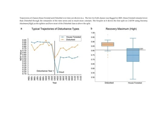
1. Introduction
The forested landscape in the Commonwealth of Virginia is being dramatically changed due to an increase in exurban development. Based on US Census data, the Washington DC metro area has 11 counties with at least one-fifth of their residents living in exurban areas [1]. Berube et al. defined exurban areas as communities located on the urban fringe that have at least 20 percent of their workers commuting to jobs in an urbanized area, exhibit low housing density, and have relatively high population growth [1]. Since 1990 population and migration gains in non-metropolitan counties have continued to increase [2,3,4].
With respect to forest management, previously undisturbed forested areas that are being intermixed with development become more difficult to manage, disrupt ecosystem services, and increase risk. Helms says a forest is “an ecosystem characterized by a more or less dense and extensive tree cover…” which if intermixed with development is no longer a forest in that sense [5] (p. 70). The wildland urban interface (WUI), defined as; “…where humans and their development meet or intermix with wildland fuel”, was developed specifically to identify the increasing fire risk for homes in the forested landscape [6,7]. Together these two definitions indicate that once a residence has been built, it is no longer just forest and the management direction may need to change. Additionally, development in previously undisturbed forest increases risk of property loss, changes the landscape, and creates concerns with water quality, zoonoses (a disease communicable from animals to humans under natural conditions), habitat fragmentation, biodiversity loss, exotic species introductions, and the like [8,9,10]. Loss of forest to development is an important issue globally, as well as in the Commonwealth, and the importance of accurate information describing the nature and extent of these land cover changes over time is increasing. The Commonwealth’s forests are economically and ecologically important, and identifying where development is occurring could allow policy makers to curate specific management strategies to address future forest loss. Identifying forest loss due to low density development is currently difficult.
Satellite as well as sampling (e.g., point, plot, and line-intersecting) approaches have been used to identify land cover and its changes over time. An acknowledged limitation of these satellite- and sampling- based approaches to estimating land-cover change is that they cannot detect some significant land-use/land-management trends, and accuracy of national databases is best at the regional and national level [11,12].
Currently the Multi-Resolution Land Characteristics Consortium (MRLC) produces National Land Cover Database (NLCD) products on a five-year cycle which is a long span, temporally, to show trends at sub-regional and local levels (county and smaller) [12,13]. In addition, according to Kennedy et al. change analyses based on two-date change detection methods do not fully tap the interrelationships among many multi-temporal images [14]. Since NLCD products are at the national scale, there are constraints to improving its temporal frequency, including timely acquisition of imagery, financial costs, and analytical methodology development [13]. Given the difficulties in improving the temporal cycle, other approaches for specific user applications need consideration.
No remote sensing change detection method has solely focused on detecting low density development in forested areas, though census-based methods have been used [10]. Investigations focusing solely on low density development in forested areas using spectral change detection have not been conducted. The NLCD Impervious Surface maps are not applicable to this problem because they use an urban mask which eliminates many of the disturbances we are trying to identify. The disturbances stakeholders usually look for are typically larger spatially, such as harvests or conversion to other land cover types (non-development) or fire impact. Low density development can include larger disturbances, but often the disturbance associated with building a single family housing unit is smaller than a single 30 m × 30 m pixel or is partially in one pixel and partially in an adjacent pixel. For forest managers, the land use of the area surrounding these single pixel developments has changed while the land cover type has not. Low density development in the forested landscape has different consequences than low density development in the non-forested landscape [10].
While low density development results in conversion to mixed surface types, both pervious and impervious, new developments in impervious surface mapping are now showing promise even for low density development. Landsat time series have been used for impervious surface mapping in two principal ways. In the first, exemplified by Sexton et al. a single model relating Landsat spectral bands or various derived indices to impervious surface area can be applied to annual images through time, resulting in a time series of impervious surface area changes (typically, accretion) [15]. In the second, exemplified by Zhang et al. temporal spectral differences between impervious and pervious surfaces can be discriminated using data derived from dense Landsat time series stacks [16]. Urban expansion and related changes to ecosystem services have been the primary foci of most of these efforts, rather than low density development per se. Powell et al., however, used spectral unmixing, multiple masks, and multiple classifications along with temporal trajectories to improve the estimation of impervious surface mapping even in low development densities [17].
Remote sensing, in general, provides a vast source of data that allows us to analyze the landscape on an immense scale. As one of the most important sources of remote sensing data, the Landsat program has provided continuous data since 1972 [18]. The Landsat 5 Thematic Mapper (TM), Landsat 7 Enhanced Thematic Mapper Plus (ETM+), and Landsat 8 Operational Land Imager (OLI) sensors provide moderate resolution (30 m) imagery and enables monitoring of land cover status and change at multiple scales [18]. Landsat is an excellent tool for tracking change, based on the quality and quantity of data. The number of potential images (22) available in a given path/row per year is why this sensor is suitable for detecting forest loss. By taking advantage of all available scenes, scientists can leverage the resulting temporal richness to detect subtle changes in the landscape that cannot be detected by using only one or two scenes per year.
With respect to existing techniques, no extant technique is ideal for finding low density development in forest covered areas. While space precludes an exhaustive listing of multi-temporal change detection techniques, we did assess several likely possibilities, including shape selection, NLCD, Vegetation Change Tracker (VCT), EWMA-CD, LandTrendr, and relevant prior work by Sen et al. [12,13,19,20,21,22,23,24,25]. NLCD products are too infrequent to detect these subtle changes [12,13,14,22,23,24]. VCT, LandTrendr, and Sen’s protocol are impacted by phenological difficulties (i.e., do not ensure the maximum leaf area condition), since each typically use a single date per year [21,24,25]. LandTrendr smooths out noise to keep false disturbances from being captured, potentially eliminating subtle disturbances like low density development [14]. VCT and Sen’s efforts are susceptible to cloud contamination [20,21,24,25]. EWMA-CD may be too computationally and data intensive for many operational users at this juncture [25]. Shape selection probably holds the most promise, but given that forest disturbance and recovery differences among disturbance types often differs more in degree than in kind, further algorithm refinements may be necessary to separate low density development from other forest disturbances [19].
Many current efforts use pre- and post-disturbance vector metrics to identify disturbance type and assess vegetation recovery. One study noted that for stand replacing disturbances such as fire, estimating ecosystem recovery may be difficult due to pioneering vegetation types and that the length of time to obtain a true estimate of recovery may exceed eight years (for their study area) [26]. Another study used pre- and post-fire Landsat imagery to compute the Normalized Burn Ratio (NBR) to study burn severity and the rate of post-fire disturbance recovery [27]. A study using Landsat data focused on spectral behavior of forest degradation due to selective logging and leveraged training curves in their classification [28]. All were focused on large scale disturbances (fire and logging) but were similar in their use of recovery metrics to separate and/or identify disturbances.
A similar study assembled an interannual Landsat time series stack using the most cloud-free scenes in a given year’s growing season and found that surface mining disturbances could be separated from other disturbances by analyzing the post-disturbance recovery. Accuracy was circumscribed by remnant clouds and subtle phenological differences. The study compared objects to pixels using NDVI, the tasseled cap greenness-brightness ratio, and Landsat TM band 3. They developed a program to automate the derivation of three diagnostic spectral trajectory variables (disturbance minimum, recovery maximum, and recovery slope) and the year of disturbance for both pixels and objects [21]. The study concluded that objects enabled more accurate identification of mine disturbances, in part because of the greater variance in pixel-based recovery trajectories, they also indicated that NDVI was the best of the three indices tested when pixels were used as the analysis unit [21].
Anthropogenic forest disturbance (especially in the actively managed forests of the U.S. Southeast) often occurs in the form of forest thinning or harvesting activities and does not necessarily result in land use change. However, some forest disturbance is the precursor to land use change (typically, to agriculture or developed classes). Once a forest disturbance is detected, examination of data from the post-disturbance period enables separation of land use change from changes related to forest management [21]. Using an object-based approach to detect low density residential development using moderate resolution earth resource satellite data has the potential to enable detection of land clearing development such as subdivisions. However, pixels are better suited for identification of smaller disturbances (i.e., single housing units).
The objective of this study was to develop a straightforward and easily implemented method by which forest loss due to low-density development can be mapped accurately using multi-temporal Landsat data. We developed a program to extract disturbance and recovery metrics with which we could model. We leveraged other indicators of low-density residential development, such as well permits and known housing starts, to develop and ensure the quality of our training and validation data.
2. Materials and Methods
2.1. Study Area
The study area is inclusive of all counties and municipalities within the Commonwealth of Virginia as shown in Figure 1. Between 1990 and 2010 the Commonwealth of Virginia has seen a 21% increase in total population as well as a 17.7% increase in rural housing units [29]. As of 2011, the Commonwealth of Virginia had 15.9 million acres of forest, which covers 62% of its land area [30]. A majority (82%) of Virginia’s forest land was privately owned making development of these privately owned forests a concern to state forest managers [30]. Other than development, the Commonwealth has experienced other forms of disturbance such as forest harvests and conversion to agriculture. With no prior information on degree of forest impacted by rural housing starts in forested areas, this study attempts to separate that development from all other disturbance types.
2.2. Automated Disturbance Detection and Diagnostics (D3) Program Development
The Virginia Tech Disturbance Detection and Diagnostics (D3) Program (which can be found at doi:10.7294/W4FB513G) was developed to automate the process of detecting disturbances to the forested landscape through the use of thresholding and parameter extraction. The code for the program is in Appendix B. This program builds off a program originally developed to identify mining disturbances and recovery trajectories [17]. For our investigation, we used the recovery trajectory tracking and added variables that were better suited to detect small disturbances on a pixel-by-pixel basis.
2.3. Landsat Data
Landsat-5 TM was the predominant source of our data. Landsat-7 ETM+, was not used for scenes after 31 May 2003 due to the scan line corrector (SLC) failure. Images used were from the WRS-2 path/rows. All available L1T images from the above two Landsat sensors with 10% cloud cover or less were acquired for the dates 1995–2011 over the Commonwealth of Virginia. If there were fewer than three images with less than 10% cloud cover in each growing season, we selected additional images up to 40% cloud cover if those images initially appeared to have cloud free pixels where our other images were obscured. The year 1995 was chosen as the study start date, as it was the earliest year we could accurately verify our validation data set using Google Earth. The surface reflectance (bottom of atmosphere) products from the Landsat Ecosystem Disturbance Adaptive Processing System (LEDAPS v. 1.0.0) were used [31].
2.4. Initial Satellite Data Processing
The analysis for the Commonwealth of Virginia consisted of 1326 unique scenes. Each acquired image was subjected to sequential processes that included converting to NDVI, removing irrelevant values (NDVI values <0 and >1 recoded as NODATA), stacking the individual NDVI images by year within a specific path/row, and extracting the maximum value per pixel per year.
For the initial scene 16/34 we processed 193 unique scenes between 1995 and 2011 (which included scenes well outside the growing season) to determine the requirements for the remainder of the study area. This path/row used all available reasonably cloud-free scenes to ensure non-growing season images did not affect the maximum value in any way. We defined the growing season as March through September. Scene 16/34 was chosen as the initial scene because it was representative of the differing terrains within the Commonwealth. The normalized difference vegetation index (NDVI) [32] was computed for each image. Each yearly stack was processed to extract the maximum NDVI value for all pixels. This resulted in 17 one-layer images, which were combined into one 17-layer image (a 98.7% data reduction).
2.5. Classification Scheme
Our goal was to distinguish disturbances caused by development from all other disturbance types at the single pixel level, and to date each disturbance. This necessitated separating disturbance due to development (“permanent” forest conversion) from other types of forest disturbances (i.e., those that did not result in permanent loss of forest). Development Disturbed (the final target class) was defined as a disturbance that resulted in a permanent change to the forest land cover that is observed to be development. In low density developed areas, our principal focus, this class includes not only new (impervious) houses but also areas around new houses (both pervious and impervious) which vary in size due to choices of the property owner. Non-Development Disturbed was broadly defined as any other disturbance to the forest land cover that was not due to development. This classification was applied to pixels by identifying each type of disturbance and then classifying them as either Development Disturbed or Non-Development Disturbed. The latter, once identified, was considered merely a temporary change to forest cover and was not separately validated (see Section 2.7).
2.6. Training Dataset
Development of a training dataset required two sources of spatially specific ancillary data. The first dataset was comprised of all well permits issued for the Commonwealth of Virginia. Permit records were obtained through the Virginia Department of Health for the years 2000–2013, acquired on 12 March 2013. The second dataset is from commercial sources DataQuick and Core Logic. This second dataset is a list of all housing starts within the Commonwealth of Virginia from 1990 to present as of the acquisition dates; 4 November 2014 and 4 June 2015.
Low density developments in forested areas do not typically have access to a public water source. Requiring access to water, all new residences have to apply for a well permit through the Virginia Department of Health (VDH) and the Commonwealth keeps all permit records. They are also required to follow specific sewage disposal regulations that require additional vegetation removal, improving detectability at Landsat resolution [33].
The wells dataset is valuable in and of itself for locating low-density residential development. However, most geocoded points are along roads, and the actual disturbances (home and adjacent clearing) are usually located well off the road, which means that unless each geocoded point is moved to the actual disturbance, very few of those points are spatially co-located with the disturbance. The wells dataset also cannot identify the size of disturbance. In addition, some rural developments may share a community well, which prohibits identification of all homes within that development by merely using well permits. An additional shortfall of datasets like this is that they are not inclusive of all counties or areas. There are quite a few counties missing from this dataset as seen in Figure 2.
Our second dataset supplements the former by identifying all residential housing starts within the Commonwealth of Virginia. It provides the date of initial construction and the site address in addition to other information. Every new residence is required to have a construction permit from the county in which it resides. No state entity exists that collates or tracks these permits, and not all counties keep electronic records that are easily accessible. DataQuick and Core Logic provided the data in its collated form for all counties from using the available data. This resulted in over 5 million records. Unfortunately, some counties in the Commonwealth lacked any housing start information, as seen in Figure 2. However, access to housing start data enabled identification of new houses even when the new construction did not require a well permit (i.e., city water or community well).
There were 696,947 housing starts, and 61,320 well permits, that were within the temporal range. The difference in volume between the datasets is due to the fact that housing starts include those that are connected to municipal water sources as well as difference in reporting requirements between the two datasets. Approximately half of the well permits were excluded because the location on the permit was not an address that could be geocoded. Therefore, these datasets could not exclusively track all low density developments. The cost of a commercial data source on housing starts is also prohibitive, especially when it lacks coverage for the entire Commonwealth. Combined, however, these two data sets provide an excellent source of sample points.
NLCD’s 1992 forest cover (legend numbers: 41 Deciduous Forest, 42 Evergreen Forest, 43 Mixed Forest, and 90 Woody Wetland) was used as the starting point for known forest [34] (p. 651). We extracted our sample points from the 1992 NLCD forest layer since our own outputs were not yet available.
A total of 1800 random sample points were selected for training and validation. 600 were selected using the well and housing start data and 1200 were selected using random points generated in ERDAS Imagine. The process of validating each XY location using Google Earth historical imagery (reliable imagery dating back to 1994–1995) required well over 100 h of effort. Any point that could not be accurately validated due to lack of clear imagery was discarded, resulting in a dataset that contained 1531 verified sample points. Each point, if not directly over a disturbance, was moved to the disturbance (middle of the main building’s roof), as some of the geocoded addresses were located over a road and not the pertinent disturbance.
290 of the 1531 verified sample points were confirmed as Development Disturbed. Of the remaining 1241 points, 848 were useable as Forest (used as baseline for forest over the time series) and 176 were useable as Non-Development Disturbed (omitted points fell in categories like water and agriculture despite their NLCD classification as forest). The resulting data set had 1314 samples (290 Development Disturbed, 848 (Persistent) Forest, and 176 (other) Non-Development Disturbed. These sample points were intersected with the mosaic stack of NDVI maxima per year so that each sample had a category and an associated 17-year (1995–2011) vector.
2.7. Implementation of D3 to Detect Forest Disturbance
We identified four different thresholds that were essential to D3. These were Vegetation Threshold, Disturbance Threshold, Cloud Threshold, and Next Year Threshold. Similar to the disturbance detection algorithm used by Sen et al., we identified a disturbance threshold where ~90% of our training data for Development Disturbed would be identified as such [21]. The Vegetation Threshold was set to keep non-forest locations out of our analysis. The Cloud Threshold was set to help eliminate possible remnant clouds. The Next Year Threshold was set to help curb wrongly identifying a pixel as being disturbed.
Using the 848 Forest sample points (and the mosaic stack of NDVI maxima per year from 1995 to 2011) we heuristically identified an NDVI value of 0.77 as the Vegetation Threshold for forest cover (i.e., pixels with an NDVI value at or above 0.77 for at least three years (the Minimum # of Years at Vegetation Threshold) were considered to have been forest at some point in the study period). We are confident in our threshold selection because we verified, using historical photography on Google Earth Pro (©2013 Google Inc., Menlo Park, CA, USA), that nearly all our known samples with an NDVI value of 0.77 were forest, but we are aware that there are forest pixels in the study area that may have been below this threshold but still forest. In a similar fashion, the disturbed (Development Disturbed + Non-Development Disturbed) sample points were used to set the Disturbance Threshold at 0.76 (in other words a pixel whose lowest NDVI value was below 0.76 was considered to be potentially disturbed). However, if the NDVI value in the year following a potential disturbance is above the Next Year Threshold (0.81, also heuristically determined) the tentative disturbance flag is removed and the pixel is not considered to be disturbed at the initially flagged time. Most disturbances, of course, had NDVI values far below 0.76, but some low density developments in previously forested areas are very subtle. As such, our Disturbance Threshold is necessarily higher than values commonly used for stand replacing disturbances.
In addition to selecting scenes to minimize cloud cover we also addressed cloud and cloud shadow contamination by programming in a Cloud Threshold. We heuristically set the Cloud Threshold at 0.4 which eliminated values below 0.4 from being considered the disturbance. If the lowest value was below 0.4, the next smallest value in the time series was checked to see whether it was both below the Disturbance Threshold and above the Cloud Threshold, and so on, up to the Number of Low Values Searched (3). This presupposes, of course, that a pixel is not obscured by clouds more than four years in the time series, which was borne out in practice given the stringent scene selection guidelines.
2.8. Interclass Differences in Disturbance and Recovery Dynamics
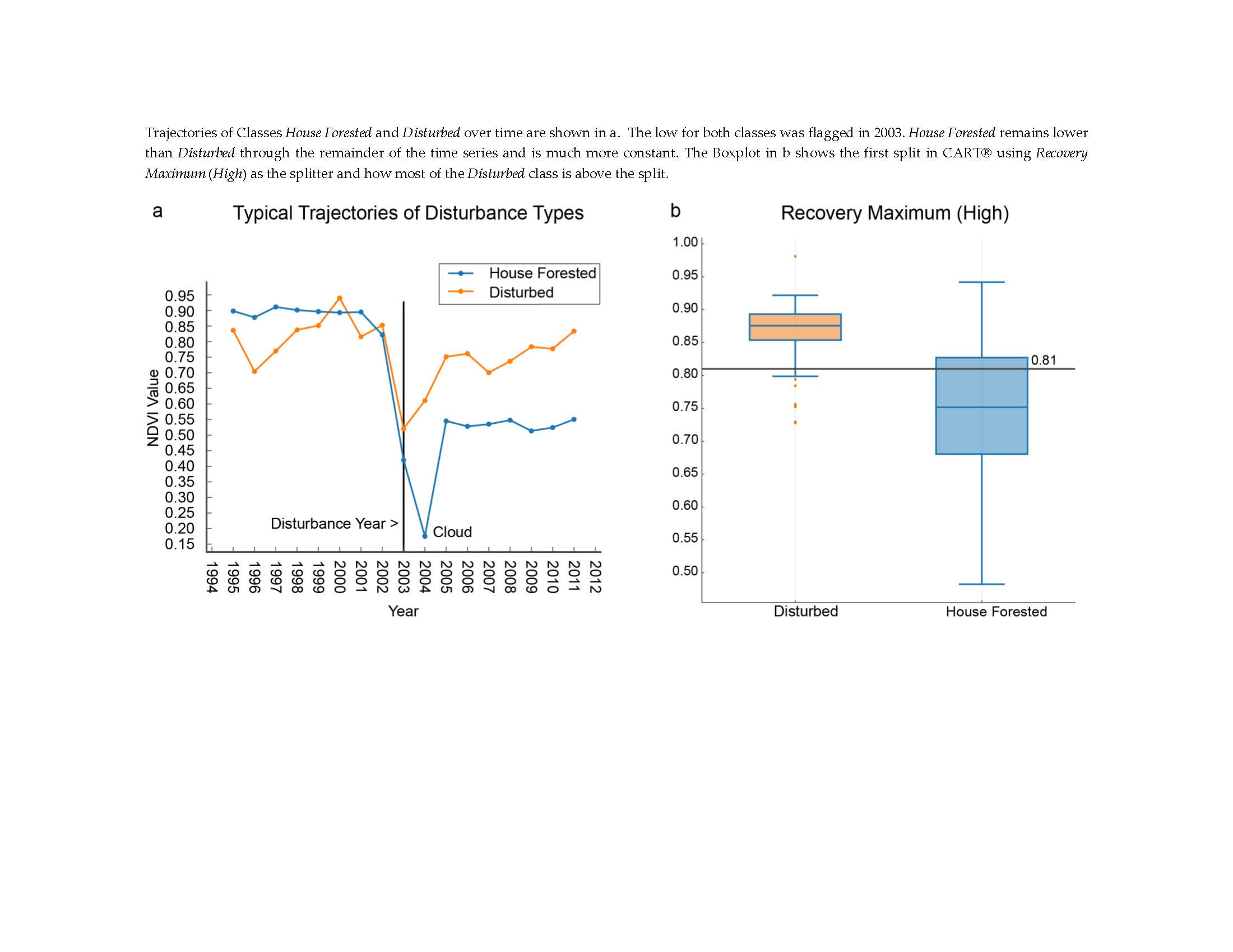
Most disturbances other than Development Disturbed are forest harvests, and the disturbed areas are either replanted for future harvests or are left to naturally revegetate. Preliminary analysis of initial NDVI trajectories, coupled with findings from previous studies, indicated that the difference in revegetation trajectories would likely allow separation of the two disturbance classes [21]. At the onset of the disturbance, both classes’ NDVI values drop dramatically as shown in Figure 3. However, as also shown in Figure 3, Development Disturbed as a class typically recovers to a lower Recovery Maximum (High) NDVI value. This representation is typical for the classes, but is not inclusive due to location of the identified low value and other false low values attributed to clouds.
We tested six variables, of which three (Minimum NDVI Value (low), Recovery Slope (low to high), and Recovery Maximum (high)) were similar to ones found in Sen et al. [21]. Additionally, we identified three new variables (Average of First Three Recovery Years, Slope over First Three Recovery Years, and Average of Three Lowest NDVI Values), all six are shown in Figure 4. Minimum NDVI Value (low) was similar to the one found in Sen et al.; however, it was not necessarily the absolute minimum (due to use of the Cloud Threshold and the Next Year Threshold potentially causing the program to select the second to fourth lowest value) [21]. Recovery Slope (low to high) and Recovery Maximum (high) in this study differ from Sen’s, in that they are not constrained to a specified number of years (17). The Recovery Maximum (high) can be any location after the identified low in the time series and the Recovery Slope (low to high) is computed from the identified low to the Recovery Maximum (high). The three new variables were derived from careful examination of differences pre- and post-disturbance that appeared to enable separation of low density residential development from other forest disturbances.
2.9. Developing a CART Model from the D3 Program Output
Using the 17-year NDVI time series and D3 (further detailed in Appendix A) a subset of the original training and validation sample in Development Disturbed and Non-Development Disturbed classes was created to examine homogeneous pixels (as assessed using historical orthophotography on Google Earth) flagged as disturbed by D3 and excluding disturbances that occurred in the final three years of the time series (to ensure calculation of Slope over First x Post Disturbance Years and Average of x Post Disturbance Years). This subset contained 166 Non-Development Disturbed samples and 197 Development Disturbed samples. From the D3 output image, values for the subset of points were extracted resulting in a table of values by layer as follows: (1) Year Disturbed, (2) Recovery Slope (low to high), (3) Slope over First Three Recovery Years, (4) Minimum NDVI Value, (5) Recovery Maximum (high), (6) Average of First Three Recovery Years, and (7) Average of Three Lowest NDVI Values. These sample points underwent recursive binary splitting in CART® using classification tree program defaults (ver.6.6, Salford Systems, San Diego, CA, USA) using layers 2, 3, 5, 6, & 7 as the predictor variables and class (House Forested and Disturbed) as the target. The best tree with a relative cost of 0.281 (classification error relative to tree size) used only two predictor variables, the Recovery Maximum (high), and the Recovery Slope (low to high), as shown in Figure 4.
2.10. Validation
A validation dataset was created to test the accuracy of the effort. Low density developments in the Development Disturbed class, our focus, are inherently rare and a completely random sample would have required an overly large number of points to identify enough validation points in this class. Further, since the class is very rare, overall accuracies would have been biased upward because of the relative ease of identifying the predominant class in the scheme, forest that is not lost to development. To pare down the effort and still remain random, we selected all addresses from the housing start dataset and sampled around them. Each XY point from this dataset is geocoded to the estimated center of the property, not necessarily the built structure itself.
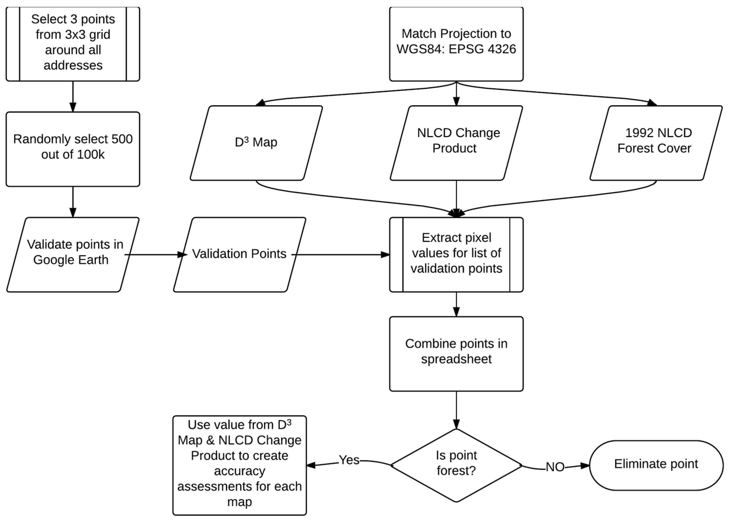
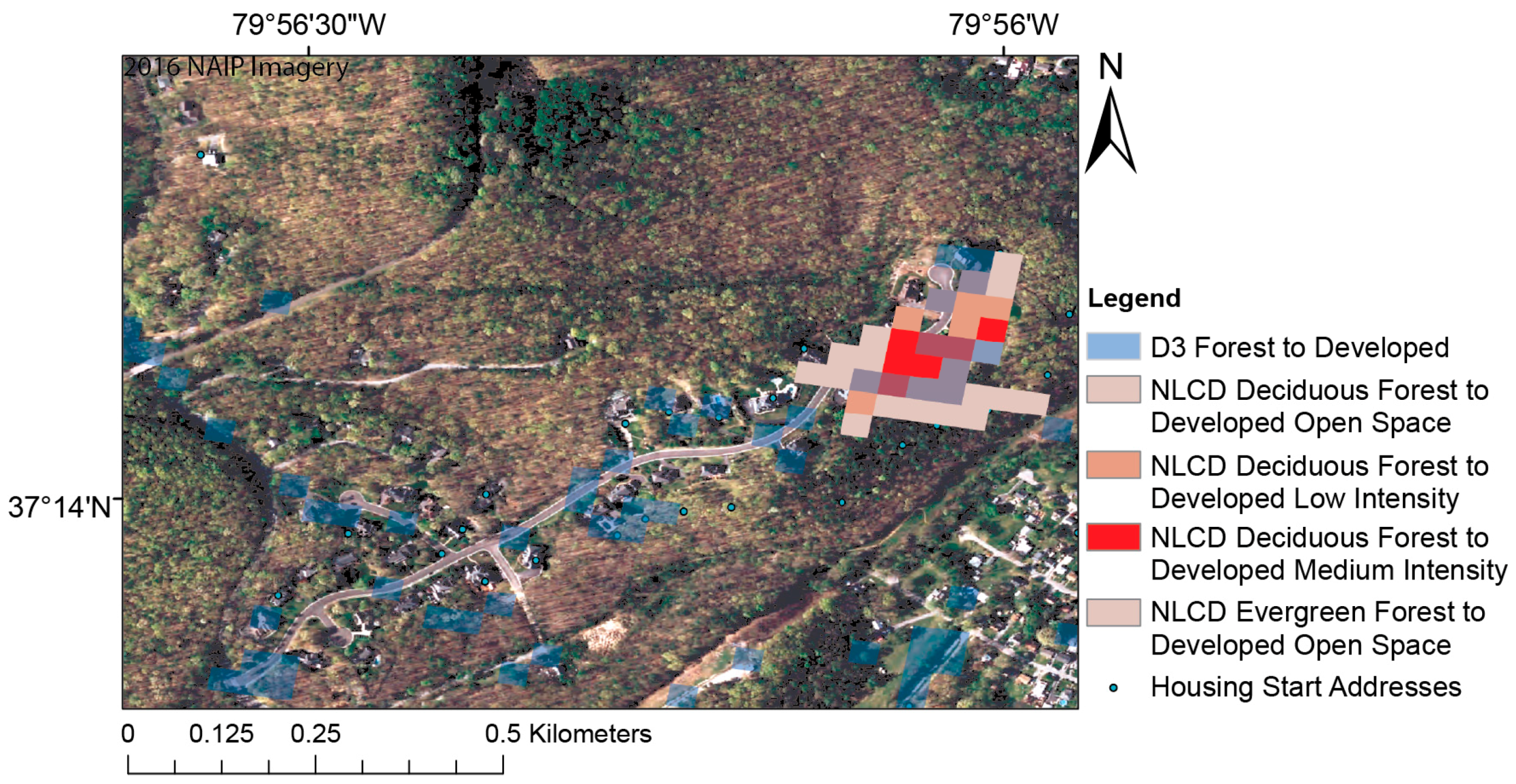
Using ArcMap 10.1 and known housing start addresses we created a raster image of zeroes and ones, where each address became a pixel with a value of one and size of 30 m. Using Spatial Analyst’s Expand Tool, we grew a 3 × 3 neighborhood around each address and merged adjoining cells into unique polygons. Using these we extracted three random points per polygon, without replacement, which resulted in 104,550 points. Within those we randomly selected 500, without replacement, to validate using Google Earth historical imagery. We used ERDAS Imagine to extract the values from our map, as shown in Figure 5, the 2011 NLCD Change Product, and the 1992 NLCD Forest layer.
We kept only the points that were within the 1992 NLCD Forest layer, which resulted in 274 samples. Using two classes: Combined Forest (which includes undisturbed Forest plus Non-Development Disturbance) and Development Disturbance we created error matrices for both the D3-based CART model and NLCD Change Product [35]. Combined Forest was defined as any point that appeared to remain forest for the entire time series or any disturbance that was not due to development, as viewed in Google Earth. Development Disturbance was defined as any point that appeared to have been forest and then cleared for development. We used all intensities of the developed classes from NLCD from four classes of forest as defined by NLCD and shown in Table 1. We combined all developed and called it Development Disturbance in the error matrices for both. We calculated the F-measure for both the D3-based CART model and the NLCD Change Product, which creates a class-specific accuracy combining both precision and recall [36,37]. We let β = 1 so that the F-measure remains balanced as shown in Equation (1)F-measure formula.
3. Results
3.1. Training Dataset
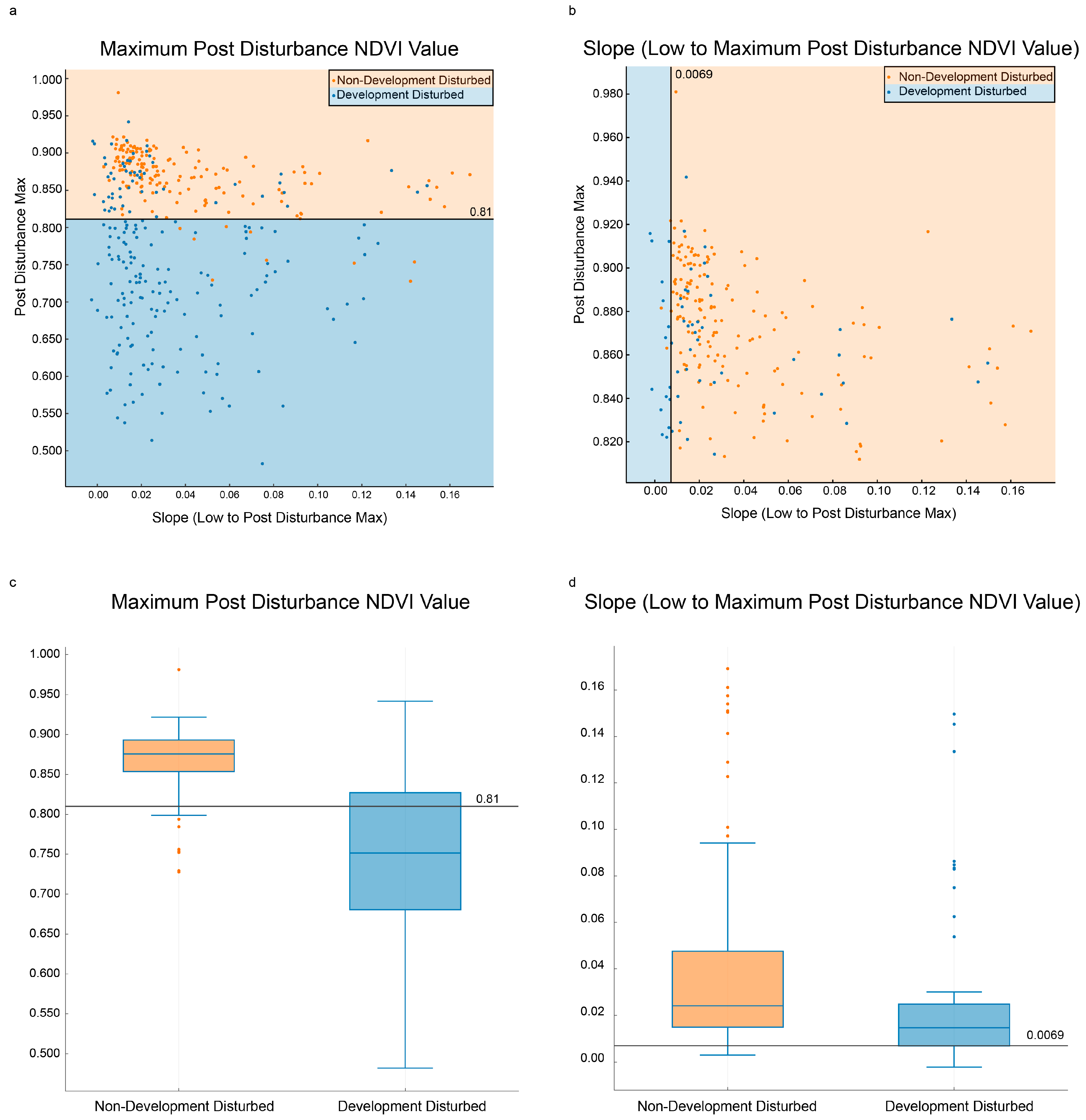
The results from CART® showed that use of two of the five predictor variables enabled the most separation between Development Disturbed and Non-Development Disturbed, as shown in Figure 6. The Recovery Maximum (High) NDVI Value was consistently higher for Non-Development Disturbed than for Development Disturbed, which supports the notion that the Non-Development Disturbed class returns to its pre-disturbed NDVI value since it is not a permanent land cover change. Development Disturbed has an average Recovery Maximum (high) value of 0.75 compared to Non-Development Disturbed’s 0.87, as seen in Figure 7.
The range in the values of the Recovery Maximum (high) of Development Disturbed (Figure 7) was larger than initially expected. This can be attributed both to the size of the disturbance and the location of the disturbance itself. If the initial disturbance was small and in a densely-vegetated area the resulting Recovery Maximum (high) would naturally be greater. Another reason for the observed large range is that the center of the house and its XY coordinate could be on the edge of a pixel resulting in some, if not most, of its clearing being in a neighboring pixel. If most of the disturbance is in a neighboring pixel, that pixel will be identified as Development Disturbed while the training point will not be. Forty (40) Development Disturbed points from our training points were misclassified as Non-Development Disturbed due to the split on High. These could not be separated using Recovery Slope (low to high).
The Recovery Slope (low to high) NDVI Value enabled separation of 15 more Development Disturbed points from Non-Development Disturbed points, with an overall tree improvement of 3.3%. These 15 points had a lower slope than the rest of the 195 sample points, which was expected. We predicted that the Non-Development Disturbed class would recover quicker than Development Disturbed. This was predicted because most forest harvests are cyclical and stakeholders have a vested interest in revegetating the harvested area as quickly as possible.
3.2. Classification Accuracy
The accuracy assessments for the D3-based CART model and the NLCD Change Product can be found in Table 2 and Table 3, respectively. The same points were extracted for both, however there were zero points that we identified as Development Disturbed in the NLCD Change Product Map. Since NLCD has a five-pixel threshold to be considered change, none of the pixels we sampled were part of a five pixel group. There were some pixels nearby that NLCD did pick up, and this is illustrated in Figure 8.
The F-measure, kappa, and overall accuracy were calculated for the Development Disturbed class for both the D3-based CART model and NLCD Change Product. The D3-based CART model had an F-measure of 0.663, a kappa of 0.5, and an overall accuracy of 77.8%. The NLCD Change Product had an F-measure of 0.0, a kappa of 0.0, and an overall accuracy of 68%.
4. Discussion
Landsat time series stacks are useful in identifying disturbances to the forested landscape, because the temporal frequency of a single Landsat satellite (this study primarily used Landsat 5 TM) is relatively high at a 16-day interval. Others have been able to further increase the temporal frequency by blending data from different satellite platforms (Landsat and MODIS) as well as using data from two Landsat satellites [38,39]. With the addition of Sentinel satellites the frequency can be increased even further and can be used to identify and quantify forest disturbances with Landsat sensors or on their own [39].
Analyses using Landsat time series stacks have been used successfully by others to identify forest disturbance. Typically, these analyses used annual (one image per year) or biennial (one image per two years) Landsat time series stacks which required the researcher to be cognizant of cloud contamination and subsequent elimination [20]. By using as many images available that were relatively cloud free, we have demonstrated that we can accurately separate disturbances due to development from other forest disturbances without the use of a spatially explicit cloud detection algorithm.
Using recovery trajectories from flagged disturbances enables us to separate disturbance types. Like Schroeder et al. (2017) both our disturbed classes have recovery trajectories that resemble a ‘vee’ shape [40]. However, even though the shape is similar, we showed that development disturbance can be separated from non-development disturbances using measurable differences in the Recovery Slope (low to high) and Recovery Maximum (High), focusing solely on post-disturbance (aka “post-rate”) spectral change. Schroeder et al. also found that the ability to detect forest conversion was quite variable (error rates: 0–77%) across test scenes, with a relative dearth of reference data a major issue [40]. Nonetheless, like our study, they were able to separate conversion from other anthropogenic disturbances such as forest harvesting, but the specific utility of their algorithm for detecting low density forest disturbances is unknown.
Separation of Development Disturbed and Non-Development Disturbed appears possible using only the highest NDVI reached post-disturbance and the slope from the lowest (non-cloud) NDVI value to the highest NDVI value post-disturbance. We were able to separate these two types of disturbance at a moderate level of accuracy. In contrast to other studies applying an object-based approach, the disturbances we were seeking were too small [21], i.e., the size of the disturbance is at or below the resolution of the sensor. It is what others consider noise that we were interested in identifying [14,41].
Our analysis illustrates that the Recovery Maximum (high) value for Non-Development Disturbed was typically higher than Development Disturbed. For the Recovery Maximum (high) the variance in Development Disturbed was considerable, as shown in Figure 7, and could not be used alone in separating disturbance types. There are instances from our training and validation dataset identified as Non-Development Disturbed where the Recovery Maximum (high) did not recover to a value greater than 0.81. A majority of those instances are later years (2006–2008) of the time series, and thus did not have as much time to recover.
By using multiple scenes per year we could eliminate the need for precursor cloud screening (other than initial image selection). Taking the maximum NDVI per year from a number of scenes reduces cloud contamination in the final image stack. With the possibility of remnant clouds in the image stack, D3 screens out the lowest NDVI values (as they were typically clouds) and checks for other false lows as a secondary cloud screening. This is important in developing an easily implemented program for others to use. By using the lowest NDVI Value, the identified low is not always the initial year of disturbance. Future work with D3 could include retroactively tracing the trajectory back to the initial year the value fell below 0.76, which could potentially be a more accurate indicator of when a disturbance first occurred.
Training data from 2009–2011 was omitted from the CART® analysis due to the inability to calculate an adequate slope. With the addition of images from 2012 to the present, it is conceivable that these misclassified sample points could be correctly classified. Some of the disturbances misclassified as Development Disturbed (based on the Recovery Maximum (High)) were spatially located on relatively flat terrain as viewed in Google Earth. Almost half were located on the coastal plain (eastern third) of Virginia. They were not replanted within the following two years. According to the Virginia Department of Forestry, “upon harvest closure any bare soils that are highly erodible or have a slope five percent or greater shall be immediately revegetated”. It indicated no recommendation for soils on slopes of less than five percent [42,43]. Therefore, the time between harvest and replanting on the coastal plain may be longer than that of areas with steeper topography.
As for the post-classification accuracy assessment of the D3-based CART model, low density development is relatively rare in the forested landscape, which made it very difficult to obtain sufficient samples with potential impact on the sample’s representativeness. The inherently coarse nature of Landsat spatial resolution (30 m) makes identifying low density development disturbances that are smaller than a single pixel difficult. When a disturbance is smaller than one pixel or between pixels, the mixing of these pixels limit our ability to accurately identify it as a true Development Disturbance. And the validation focused, by design, on a rigorous assessment of the difficult task of how well the algorithm can detect, with minimal omission and commission, low density residential development. Qualitative evaluation of algorithm performance outside this context did not reveal any major issues (e.g., Figure 8). However, further research is needed to ensure that enabling detection of these important, but spatially and spectrally subtle, disturbances does not unduly affect the accuracy of classifying other permanent forest conversion types.
Nationally, disturbance events impact <3% of forest area per year, making any specific disturbance type rare [40,44]. As we noted earlier, Schroeder et al. also allude to the difficulty in collecting enough reference data to sufficiently capture disturbances like low density development [40]. Through the use of well permit data and housing start data we had 750 k points from which we could sample, in addition to the random points generated for the other disturbance types. Without these datasets the algorithm presented here could not have been developed or validated. Neither of these datasets had statewide coverage, but together they provided ample coverage from which to sample. The housing start data are an expensive, licensed product. In contrast, the well data are free for public use.
5. Conclusions
Using an approach that identifies a forest disturbance and evaluates its post-disturbance trajectory is an excellent method for distinguishing disturbances due to development from other causes of forest disturbance. In our analysis, the majority of the known classification errors were due to the temporal length being too short. These same techniques would have a high likelihood of even greater success with finer spatial resolution image time series stacks that will eventually be available from sensors like the Sentinel 2 MultiSpectral Instrument.
The Landsat archive contains an enormous amount of data with which these types of analyses can be run. With the archive now being free to the public, large scale, image dense analyses can be more routinely conducted. A limiting factor is the time required to acquire and process enough images per path/row to conduct an effective analysis.
Here we have demonstrated a simple and accurate way to detect forest loss due to development that allows foresters and others a new opportunity to understand where development is occurring within the forested landscape. This method can be used as an additional tool in devising a more tailored forest development management strategy.
Acknowledgments
This work was funded by the US Geological Survey Grant: G12PC00073, “Making Multitemporal Work” and the Virginia Department of Forestry: “Mapping Virginia’s Forest Conversion Hotspots”: AT-15689, Funding for R.H.W.’s participation was also provided in part by the Virginia Agricultural Experiment Station and the McIntire-Stennis Program of NIFA, USDA: “Detecting and Forecasting the Consequences of Subtle and Gross Disturbance on Forest Carbon Cycle: Project Number 1007054. We would also like to acknowledge Mike Santucci and Robert Farrell from the Virginia Department of Forestry for their guidance and support of this endeavor.
Author Contributions
Matthew House contributed to the research design, collected the data, aided in designing the program D3 and its implementation, and led the interpretation of results and manuscript writing. Randolph Wynne secured funding, proposed and developed the research design, led the D3 code development effort, helped in the interpretation of results and in manuscript writing and revisions.
Conflicts of Interest
The authors declare no conflict of interest.
Appendix A. Automated Disturbance Detection and Diagnostics (Description and Process Flow Charts)
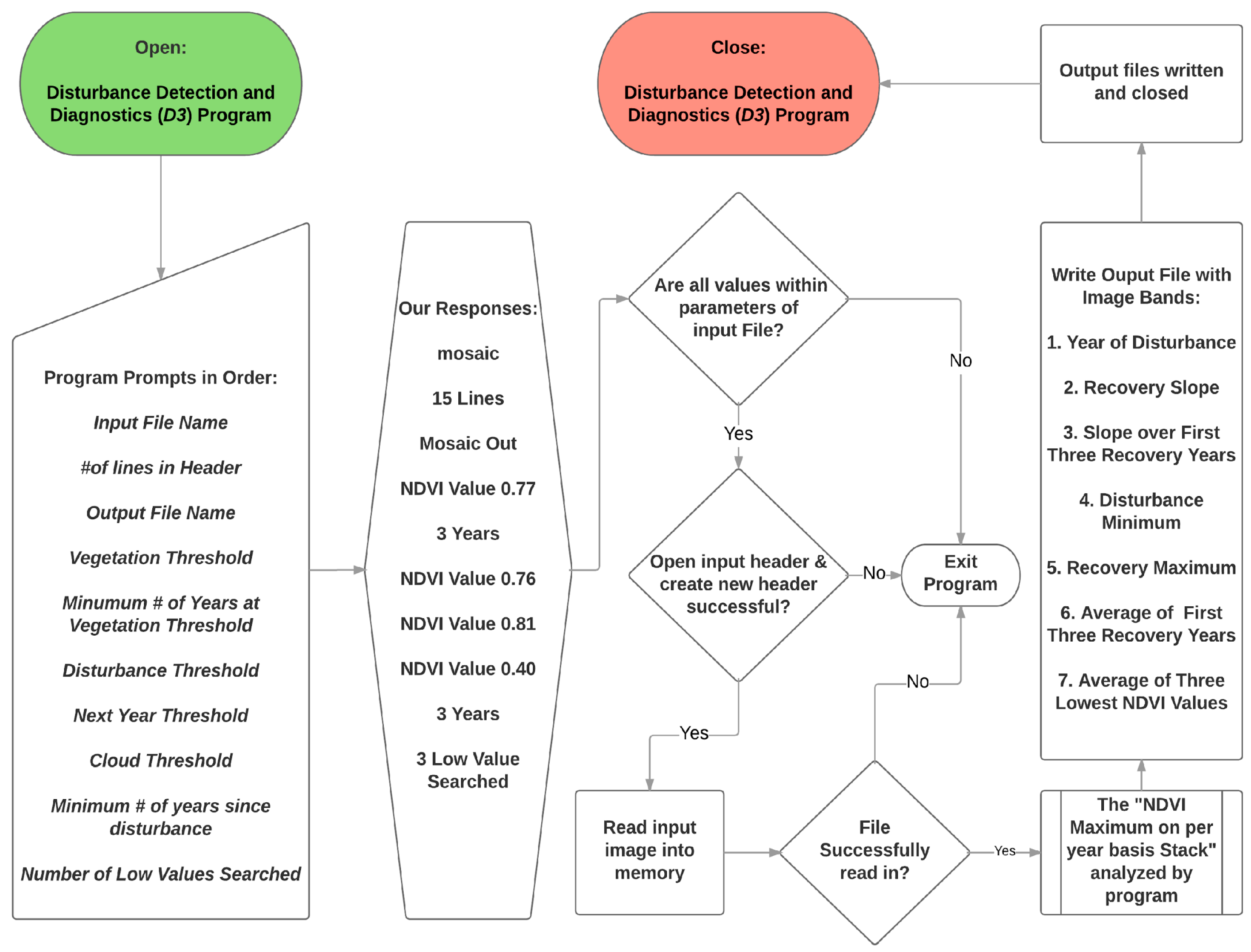
The Virginia Tech Disturbance Detection and Diagnostics (D3) Program (Figure A1 and Figure A2) is written in FORTRAN 95. The code for the program is in Appendix B. This program builds off of a program originally developed to identify mining disturbances and recovery trajectories [21]. For our investigation, we used the recovery trajectory tracking and added variables that were better suited to detect small disturbances on a pixel by pixel basis.
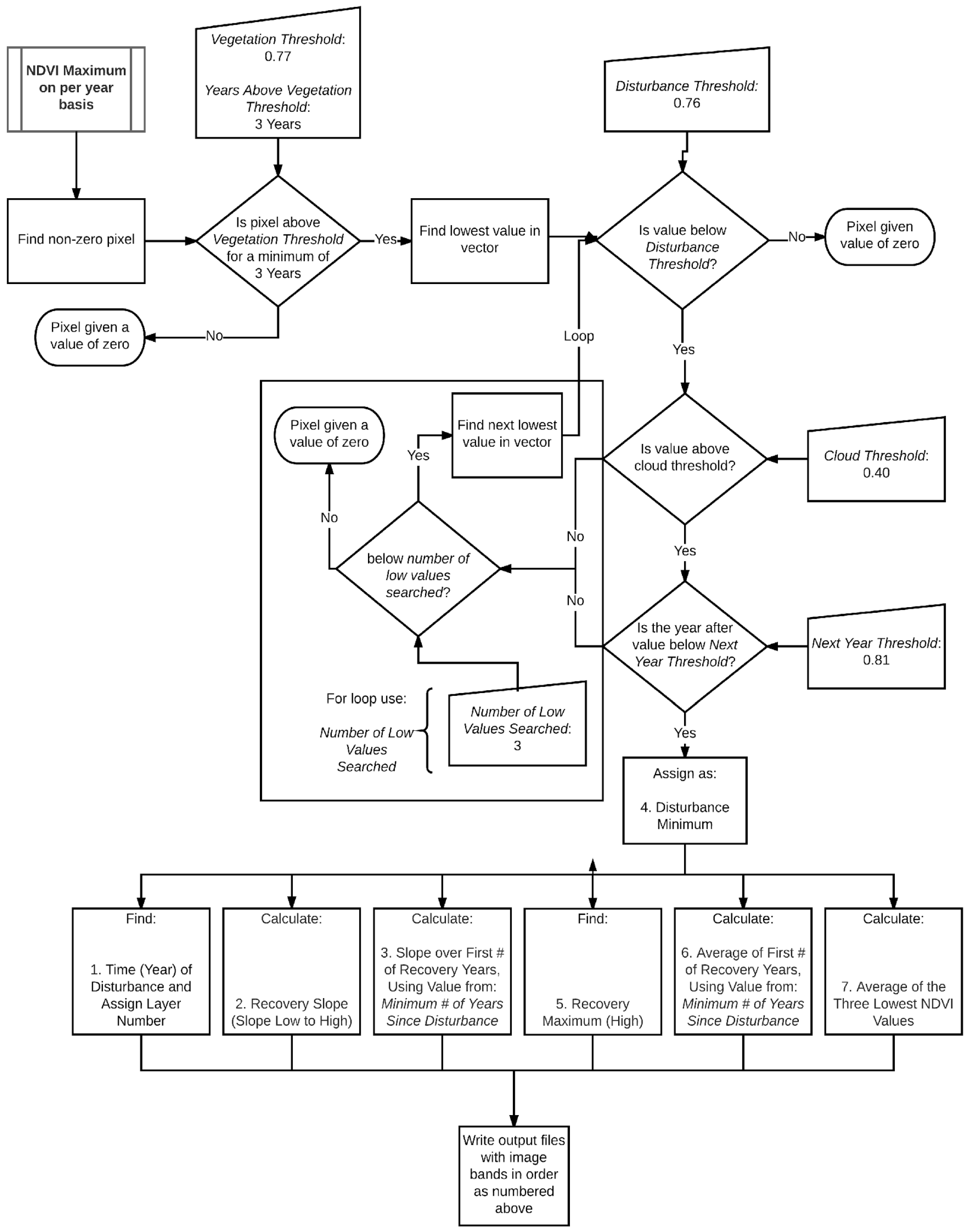
The mosaic stack of NDVI maxima per year (if it was forest in the 1992 NLCD) was the input to D3. Program flow is detailed in Figure A2, though we include a simplified overview of the process here. Required input parameters and their values are shown in Table A1 and Figure A1. To make sure that each pixel was (at least initially) forest, we ensure that the pixel exceeds the Minimum # Years at Vegetation Threshold (0.77) for at least three years (the Minimum # of Years at Vegetation Threshold), otherwise that pixel is omitted from further analysis. A pixel is (initially) considered to be disturbed if the lowest NDVI value in the time series falls below the Disturbance Threshold (0.76). To ensure false lows are not identified as disturbances, the NDVI value in the year following the flagged disturbance has to be below the Next Year Threshold (0.81). Low NDVI values due to clouds (which could be mistaken as disturbances) are removed if the NDVI value is below the Cloud Threshold (0.4).

Table A1.
User-Specified Parameters.
| D3 Input Prompts | Definition and Use |
|---|---|
| Vegetation Threshold | Pixels above this value are labeled forest/vegetation. |
| Minimum # of Years at Vegetation Threshold | A pixel must exceed the vegetation threshold a minimum of 3 years. |
| Disturbance Threshold | A pixel is considered disturbed for a year if its value falls below this threshold |
| Next Year Threshold | The pixel value for the year immediately following the identified low is used to separate false lows from a true disturbance. If the value is above the threshold the identified low is discarded and the next lowest value is considered. |
| Cloud Threshold | The identified low value cannot be below this threshold. Values below this predominantly indicate (and are assumed to be) clouds. |
| Minimum # of Years Since Disturbance | This is the number of years over which the static average and slope are computed |
| Number of Low Values Searched | This is the number of times D3 searches for a low value in a pixel time series vector. |
Diagnostics (Figure A2 and Table A2) are computed only on pixels flagged as disturbed. The only input parameter used in the computation of the output diagnostics is the Minimum Number of Years (3) Since Disturbance (Table A1) used to compute the Average of First # of Recovery Years and Slope over First # Recovery Years (Table A2).
Figure A1.
D3 Program flow chart identifying program prompts and user supplied responses as an overview of the process.
Figure A1.
D3 Program flow chart identifying program prompts and user supplied responses as an overview of the process.
The output image is comprised of seven layers as labeled in Table A2.
Table A2.
D3 Output’s 7 layers.
| Output Layers of D3 | |
|---|---|
| 1 | Year of Disturbance |
| 2 | Slope Low to High |
| 3 | Slope over First x Post Disturbance Years |
| 4 | Low (value when first fell below threshold) |
| 5 | Recovery Maximum (Highest NDVI Value after Low) |
| 6 | Average (of x Post Disturbance Years) |
| 7 | Average of Lowest Three Values in Entire Time series |
Figure A2.
Flow chart of calculations within program illustrating how it identifies a given pixel as disturbed or undisturbed, and, if disturbed, what derived indices were calculated.
Figure A2.
Flow chart of calculations within program illustrating how it identifies a given pixel as disturbed or undisturbed, and, if disturbed, what derived indices were calculated.

Appendix B. Fortran Code for Virginia Tech Disturbance Program (D3)
! ENVI Standard BSQ i/o
! Finds potential forest disturbance and calculates recovery metrics
!
!
! Randolph H. Wynne, FREC, Virginia Polytechnic Institute and State University
! Susmita Sen, FREC, Virginia Polytechnic Institute and State University
! Matthew House, FREC, Virginia Polytechnic Institute and State University
!
! Version 10, 02-Aug-16
!
program D3
use SVRGP_INT
implicit none
LOGICAL :: PixelNotWritten
LOGICAL :: NextYearAlsoDisturbed = .FALSE.
LOGICAL :: YearDisturbedIsLastYear = .FALSE.
LOGICAL :: FoundDisturbance = .FALSE.
LOGICAL :: OS = .FALSE.
LOGICAL :: Printed = .FALSE.
LOGICAL :: FirstSecondLow = .TRUE.
INTEGER, parameter :: REALKIND = 4, S_LEN = 32, STRINGBUFFER = 500, NEG1 = −1
INTEGER, parameter :: OUTNUMBANDS = 7
INTEGER (KIND = 8), parameter :: TEST_PIXEL = 20017380
INTEGER (KIND = 2) :: b ! NumBands
INTEGER (KIND = 2) :: IndexValue = 1
INTEGER (KIND = 2) :: MinRecoveryYears
INTEGER (KIND = 2) :: RecoveryYear
INTEGER (KIND = 2) :: MinYearsVegetation
INTEGER (KIND = 2) :: YearDisturbed = 0
INTEGER (KIND = 2) :: MinimumLocation = 0
INTEGER (KIND = 2) :: NumHeaderLines = 0
INTEGER (KIND = 2) :: CurrHeaderLineNum = 7
INTEGER (KIND = 2) :: NumLowValuesSearched
INTEGER (KIND = 8) :: Currx, Currx_fixed
INTEGER (KIND = 8) :: NumRecoveryYears
INTEGER (KIND = 8) :: NumRows, NumCols
INTEGER (KIND = 8) :: i, j, k, l, m, PostDisturbYear, LowValue ! Loop counters
INTEGER (KIND = 8) :: InRecLen, OutRecLen
REAL (KIND = 4) :: Threshold
REAL (KIND = 4) :: NextYearThreshold
REAL (KIND = 4) :: CloudThreshold
REAL (KIND = 4) :: Vegetation
REAL (KIND = 4) :: sxx, sxx_fixed
REAL (KIND = 4) :: sxy, sxy_fixed
REAL (KIND = 4) :: xm, xm_fixed
REAL (KIND = 4) :: ym, ym_fixed
REAL (KIND = 4) :: xsum, xsum_fixed
REAL (KIND = 4) :: ysum, ysum_fixed
REAL (KIND = 4) :: ysumshort !for recovery years only
REAL (KIND = 4) :: xres, xres_fixed
REAL (KIND = 4) :: yres, yres_fixed
REAL (KIND = 4) :: PixelSlope, PixelSlopeFixed
REAL (KIND = 4) :: CurrMax, CurrMin !,CurrValue, PrevValue, NextValue
REAL (KIND = 4) :: MinOne, MinTwo, MinThree
INTEGER (KIND = 4), ALLOCATABLE :: Indices (:)
REAL (KIND = 4), ALLOCATABLE :: UnsortedVector (:)
REAL (KIND = 4), ALLOCATABLE :: SortedVector (:)
REAL (KIND = 4), ALLOCATABLE :: x (:,:)
INTEGER (KIND = 4), ALLOCATABLE :: When (:)
REAL (KIND = 4), ALLOCATABLE :: WhenReal (:)
REAL (KIND = 4), ALLOCATABLE :: Slope (:)
REAL (KIND = 4), ALLOCATABLE :: Low (:)
REAL (KIND = 4), ALLOCATABLE :: High (:)
REAL (KIND = 4), ALLOCATABLE :: Average (:)
REAL (KIND = 4), ALLOCATABLE :: RecovPeriodSlope (:)
REAL (KIND = 4), ALLOCATABLE :: Forest (:)
REAL (KIND = 4), ALLOCATABLE :: AvgThreeMins(:)
CHARACTER (LEN = 4) :: ENVI = "ENVI"
CHARACTER (LEN = S_LEN) :: InputFileName
CHARACTER (LEN = S_LEN) :: InputHeaderFileName
CHARACTER (LEN = S_LEN) :: AbsoluteFileName
CHARACTER (LEN = S_LEN) :: AbsoluteHeaderFileName
CHARACTER (LEN = STRINGBUFFER) TempString
! The command line prompts in “” begin once D3 is called in command line interface on a
! windows desktop machine
PRINT *, “Input file name: ”
read (unit = *, FMT = *) InputFileName
PRINT *, “Number of lines in header: ”
read (unit = *, FMT = *) NumHeaderLines
PRINT *, “Output file name: ”
read (unit = *, FMT = *) AbsoluteFileName
PRINT *, “Vegetation threshold: ”
read (unit = *, FMT = *) Vegetation
PRINT *, “Minimum number of years at vegetation threshold”
read (unit = *, FMT = *) MinYearsVegetation
PRINT *, “Disturbance threshold: ”
read (unit = *, FMT = *) Threshold
PRINT *, “Next year threshold: ”
read (unit = *, FMT = *) NextYearThreshold
PRINT *, “Cloud threshold: ”
read (unit = *, FMT = *) CloudThreshold
PRINT *, “Minimum number of years since disturbance: ”
read (unit = *, FMT = *) MinRecoveryYears
PRINT *, “Number of low values searched: ”
read (unit = *, FMT = *) NumLowValuesSearched
InputHeaderFileName = TRIM (InputFileName)//“.hdr”
! InputHeaderFileName = “sm.hdr”
PRINT *, “InputHeaderFileName”
PRINT *, “”, InputHeaderFileName
AbsoluteHeaderFileName = TRIM (AbsoluteFileName)//“.hdr”
PRINT *, “OutputHeaderFileName”
PRINT *, “”, AbsoluteHeaderFileName
! last user required input is “OutputHeaderFileName”
! begin reading in header then, if successful, the input file
open (unit = 13, file = InputHeaderFileName, &
status = “old”, action = “read”)
INQUIRE (unit = 13, Opened=OS)
if (OS) then
PRINT *, “Input header file successfully opened.”
end if
open (unit = 14, file = AbsoluteHeaderFileName, &
status = “replace”, action = “write”)
open (unit = 21, file = “debug.txt”, &
status = “replace”, action = “write”)
read (unit = 13, fmt = “(A)”) TempString
write (unit = 14, fmt = *) ENVI
PRINT *, ENVI
read (unit = 13, fmt = “(A)”) TempString
write (unit = 14, fmt = “(A)”) TRIM (ADJUSTL(TempString))
PRINT *, TRIM (TempString)
read (unit = 13, fmt = “(A)”) TempString
write (unit = 14, fmt = “(A)”) TRIM (ADJUSTL(TempString))
PRINT *, TRIM (TempString)
read (unit = 13, fmt = “(A10,I5)”) TempString, NumCols
write (unit = 14, fmt = “(A10,I5)”) TRIM (TempString), NumCols
PRINT *, TRIM (TempString), NumCols
read (unit = 13, fmt = “(A10,I5)”) TempString, NumRows
write (unit = 14, fmt = “(A10,I5)”) TRIM (TempString), NumRows
PRINT *, TRIM (TempString), NumRows
read (unit = 13, fmt = “(A10,I3)”) TempString, b
write (unit = 14, fmt = “(A10,I3)”) TRIM (TempString), OUTNUMBANDS
PRINT *, TRIM (TempString), b
CopyRestofHeader: do while (CurrHeaderLineNum .LE. NumHeaderLines)
read (unit = 13, fmt = “(A)”) TempString
CurrHeaderLineNum = CurrHeaderLineNum + 1
write (unit = 14, fmt = “(A)”) TRIM (ADJUSTL(TempString))
PRINT *, TRIM (TempString)
end do CopyRestofHeader
PRINT *, “”
CLOSE(13)
CLOSE (14)
! k = 16789 * 26214
k = NumRows * NumCols
OutRecLen = k * REALKIND !NumPixels * Bytes/Real
InRecLen = k * REALKIND !NumPixels * Bytes/Real
! matches input file size to output file size
write (unit = *, FMT = *) “Input file names: ”
write (unit = *, FMT = *) “ ”, InputFileName
write (unit = *, FMT = *) “Number of Bands: ”
write (unit = *, FMT = *) “ ”, b
write (unit = *, FMT = *) “Output file names: ”
write (unit = *, FMT = *) “ ”, AbsoluteFileName
write (unit = *, FMT = *) “Record lengths (In, Out)”
write (unit = *, FMT = *) “ ”, InRecLen, OutRecLen
ALLOCATE (Indices (b))
ALLOCATE (UnsortedVector (b))
ALLOCATE (SortedVector (b))
ALLOCATE (x (k,b))
ALLOCATE (When (k))
ALLOCATE (WhenReal (k))
ALLOCATE (Slope (k))
ALLOCATE (Low (k))
ALLOCATE (High (k))
ALLOCATE (Average(k))
ALLOCATE (RecovPeriodSlope(k))
ALLOCATE (Forest (k))
ALLOCATE (AvgThreeMins(k))
x = 0.0
When = 0
WhenReal = 0.0
Slope = 0.0
Low = 0.0
High = 0.0
Average = 0.0
RecovPeriodSlope = 0.0
AvgThreeMins = 0.0
PixelNotWritten = .TRUE.
open (unit = 11, file = InputFileName, form = “unformatted”, &
access = “direct”, recl = InRecLen, status = “old”, action = “read”)
write (unit = *, fmt = *) “Reading input image into memory...”
ReadRawBandsLoop: do j = 1, b
read (unit = 11, rec = j) x (:,j)
end do ReadRawBandsLoop
close (unit = 11)
write (unit = *, fmt = *) “Input image read into memory.”
PRINT *, “Calculating absolute thresholds and slopes”
LessThanFourTenthsAbs: do i = 1, k
IndexValue = 1
do m = 1, b
Indices (m) = IndexValue
IndexValue = IndexValue + 1
end do
UnsortedVector = 0.0
SortedVector = 0.0
NextYearAlsoDisturbed = .FALSE.
YearDisturbedIsLastYear = .FALSE.
FoundDisturbance = .FALSE.
MinimumLocation = 0
! If the pixel is vegetated and not a background pixel then proceed
VegPixelsOnly: if (((COUNT((x(i,:)).GT. Vegetation)) .GE. MinYearsVegetation) .AND. (MINVAL (x(i,:)) .NE. 0.0)) then
UnsortedVector = x(i,:)
CALL SVRGP (UnsortedVector, SortedVector, Indices)
! Sorts a real array by algebraically increasing value and return the permutation that rearranges
! the array.
if ((Printed .EQ. .FALSE.) .OR. (i .EQ. TEST_PIXEL)) then
PRINT *, UnsortedVector
PRINT *, “ ”
PRINT *, SortedVector
PRINT *, “ ”
PRINT *, Indices
PRINT *, “ ”
end if
Forest (i) = 2.0
CurrMax = 0.0
CurrMin = 1.0
LowValue = 1
! Find a pair of low values starting from the lowest value, then proceeding to next lowest, etc.
FindPairofLowValues: do while ((LowValue .LE. NumLowValuesSearched) .AND. (FoundDisturbance .EQ. .FALSE.))
! This is looking for the lowest value in the sorted vector and testing the value against two
! thresholds: the
! disturbance threshold and then the cloud threshold and then it checks to make sure the band(b)
! (year) is not
! the last in the series. (if b=17 then b cannot equal 17)
if ((SortedVector(LowValue) .LT. Threshold) .AND. (SortedVector(LowValue) .GT. CloudThreshold)) then
MinimumLocation = Indices(LowValue)
if ((Printed .EQ. .FALSE.) .OR. (i .EQ. TEST_PIXEL)) then
PRINT *, “SortedVector(LowValue), Threshold, CloudThreshold, Indices(LowValue)”, &
SortedVector(LowValue), Threshold, CloudThreshold, Indices(LowValue)
end if
if (MinimumLocation .EQ. b) then
YearDisturbedIsLastYear = .TRUE.
end if
if ((Printed .EQ. .FALSE.) .OR. (i .EQ. TEST_PIXEL)) then
PRINT *, “YearDisturbedIsLastYear”, YearDisturbedIsLastYear
end if
! If the year disturbed is not the last year in the number of bands (b) in the file then the program
! takes the minimum
! location and adds a (1) year to it and checks that bands value against the next year threshold. If
! below the program
! says that year is also disturbed and that it has found the true disturbance.
if (YearDisturbedIsLastYear .NE. .TRUE.) then
if (x(i,MinimumLocation + 1) .LT. NextYearThreshold) then
NextYearAlsoDisturbed = .TRUE.
FoundDisturbance = .TRUE.
When(i) = MinimumLocation
YearDisturbed = MinimumLocation
end if
end if
if ((Printed .EQ. .FALSE.) .OR. (i .EQ. TEST_PIXEL)) then
PRINT *, “NextYearAlsoDisturbed, YearDisturbedIsLastYear”
PRINT *, “FoundDisturbance, When(i), YearDisturbed”
PRINT *, NextYearAlsoDisturbed, YearDisturbedIsLastYear, FoundDisturbance, &
When(i), YearDisturbed
if (LowValue .EQ. NumLowValuesSearched) then
Printed = .TRUE.
end if
end if
end if
LowValue = LowValue + 1
end do FindPairofLowValues
! If either the cloud threshold or year after threshold are not met the program loops to test the
! next lowest
! value in the sorted vectoras long as the LowValue is less than or equal to the user defined:
! NumLowValuesSearched
LowValueOnlyIfDisturbed: if (YearDisturbed .GT. 0) then
Low(i) = x(i,YearDisturbed)
END if LowValueOnlyIfDisturbed
! Only assign a low value if a value met all qualifications of the thresholds above.
! Compute Slopes if the pixel was assigned a low value and if the year disturbed less than or
! equal to the number of
! bands minus the user defined minimum number of recovery years
TrueSlope: if ( (YearDisturbed .GT. 0) .AND. ( (b-YearDisturbed) .GE. MinRecoveryYears) ) then
if (YearDisturbed .EQ. 0) then
PRINT *, “Should not be computing slopes with no disturbance!!!”
STOP
end if
sxx = 0.0
sxx_fixed = 0.0
sxy = 0.0
sxy_fixed = 0.0
Currx = 0
Currx_fixed = 0
xm = 0.0
xm_fixed = 0.0
ym = 0.0
ym_fixed = 0.0
xsum = 0.0
ysum = 0.0
xsum_fixed = 0.0
ysum_fixed = 0.0
ysumshort = 0.0
xres = 0.0
xres_fixed = 0.0
yres = 0.0
yres_fixed = 0.0
PixelSlope = 0.0
PixelSlopeFixed = 0.0
MinOne = 0.0
MinTwo = 0.0
MinThree = 0.0
PostDisturbYear = 0
! This finds the highest value in the timeseries that occurs after the recorded low value
FindRecoveryMax: do l = YearDisturbed, b
FindMaxAfterDisturbance: if (x(i,l) .GT. CurrMax) then
CurrMax = x(i,l)
end if FindMaxAfterDisturbance
High(i) = CurrMax
RecoveryYear = l
end do FindRecoveryMax
NumRecoveryYears = RecoveryYear - YearDisturbed
! Below finds the three lowest values in the time series
MinOne = Low(i)
do l = YearDisturbed, b
if ((x(i,l) .LT. CurrMin) .AND. (x(i,l) .GE. MinOne)) then
CurrMin = x(i,l)
end if
MinTwo = CurrMin
end do
CurrMin = 1.0
do l = YearDisturbed, b
if ((x(i,l) .LT. CurrMin) .AND. (x(i,l) .GE. MinTwo)) then
CurrMin = x(i,l)
end if
MinThree = CurrMin
end do
AvgThreeMins(i) = (MinOne+MinTwo+MinThree)/3.0
CalculateSums: do l = YearDisturbed, RecoveryYear
PostDisturbYear = PostDisturbYear + 1
Currx = Currx + 1
xsum = xsum + Currx
ysum = ysum + x(i,l)
if (PostDisturbYear .EQ. MinRecoveryYears) then
xsum_fixed = xsum
ysum_fixed = ysum
end if
!
end do CalculateSums
CalculateSumMinRecoveryYears: do l = YearDisturbed+1, YearDisturbed + MinRecoveryYears
ysumshort = ysumshort + x(i,l)
end do CalculateSumMinRecoveryYears
! Calculate means
xm = xsum/(NumRecoveryYears)
ym = ysum/(NumRecoveryYears)
! Below computes the slope over the minimum number of recovery years.
Average(i) = ysumshort/MinRecoveryYears
Currx = 0
ComputeVarSlopePrecursors: do l = YearDisturbed, &
RecoveryYear
Currx = Currx + 1
xres = Currx − xm
yres = x(i,l) − ym
sxx = sxx + (xres * xres)
sxy = sxy + (xres * yres)
end do ComputeVarSlopePrecursors
ComputeFixedSlopePrecursors: do l = YearDisturbed + 1, YearDisturbed + MinRecoveryYears
Currx_fixed = Currx_fixed + 1
xres_fixed = Currx_fixed - xm_fixed
yres_fixed = x(i,l) − ym_fixed
sxx_fixed = sxx_fixed + (xres_fixed * xres_fixed)
sxy_fixed = sxy_fixed + (xres_fixed * yres_fixed)
end do ComputeFixedSlopePrecursors
PixelSlopeFixed = sxy_fixed/sxx_fixed
PixelSlope = sxy/sxx
Slope(i) = PixelSlope
RecovPeriodSlope(i) = PixelSlopeFixed
end if TrueSlope
end if VegPixelsOnly
YearDisturbed = 0
END do LessThanFourTenthsAbs
! Program finished, now begin writing output file and header
PRINT *, “Absolute processing completed.”
PRINT *, “First year set to zero for both absolute and difference.”
PRINT *, “Opening output files.”
open (unit = 10, file = AbsoluteFileName, form = “unformatted”, &
access = ‘direct’, recl = OutRecLen, status = “replace”, action = “write”)
write (unit = *, fmt = *) “Output image files opened.”
write (unit = *, fmt = *) “Writing output files.”
WhenReal = REAL(When)
write (unit = 10, rec = 1) WhenReal
write (unit = 10, rec = 2) Slope
write (unit = 10, rec = 3) RecovPeriodSlope
write (unit = 10, rec = 4) Low
write (unit = 10, rec = 5) High
write (unit = 10, rec = 6) Average
write (unit = 10, rec = 7) AvgThreeMins
PRINT *, “Output image successfully written.”
PRINT *, “ ”
PRINT *, “Output image band order:”
PRINT *, “ Year of Disturbance”
PRINT *, “ Slope to Maximum Post-Recovery Value”
PRINT *, “ Slope over MinRecoveryYears”
PRINT *, “ Low (value when first fell below threshold)”
PRINT *, “ High (highest value within specified recovery period)”
PRINT *, “ Average (in post mining recovery period)”
PRINT *, “ Average of lowest three values in entire time series”
PRINT *, “ ”
close (unit = 10)
close (unit = 12)
close (unit = 21)
write (unit = *, fmt = *) “Output files written and closed.”
write (unit = *, fmt = *) “D3 complete.”
end program D3
References
- Berube, A.; Singer, A.; Wilson, J.H.; Frey, W.H. Finding Exurbia: America’s Changing Landscape at the Metropolitan Fringe; The Brookings Institution: Washington, DC, USA, 2006. [Google Scholar]
- Johnson, K.M.; Beale, C.L. The recent revival of widespread population growth in nonmetropolitan areas of the United States. Rural Sociol. 1994, 59, 655–667. [Google Scholar] [CrossRef]
- Johnson, K.M.; Cromartie, J.B. The rural rebound and its aftermath. Popul. Chang. Rural Soc. 2006, 25–49. [Google Scholar] [CrossRef]
- Perry, M.J.; Mackun, P.J.; Joyce, C.D.; Lollock, L.R.; Pearson, L.S. Population change and distribution. Montana 2001, 799, 103–130. [Google Scholar]
- Helms, J.A. The Dictionary of Forestry, 2nd ed.; Society of American Foresters: Bethesda, MD, USA, 1998; ISBN 978-0939970735. [Google Scholar]
- Glickman, D.; Babbitt, B. Urban wildland interface communities within the vicinity of federal lands that are at high risk from wildfire. Fed. Regist. 2001, 66, 751–777. [Google Scholar]
- Cohen, J.D. The wildland-urban interface fire problem: A consequence of the fire exclusion paradigm. In Forest History Today; U.S. Forest Service: Washington, DC, USA, 2008; pp. 20–26. [Google Scholar]
- Zoonoses in Merriam-Webster. 2017. Available online: https://www.merriam-webster.com/dictionary/zoonoses (accessed on 7 July 2017).
- Radeloff, V.C.; Hammer, R.B.; Stewart, S.I.; Fried, J.S.; Holcomb, S.S.; McKeefry, J.F. The wildland-urban interface in the United States. Ecol. Appl. 2005, 15, 799–805. [Google Scholar] [CrossRef]
- Stein, S.M.; McRoberts, R.E.; Alig, R.J.; Nelson, M.D.; Theobald, D.M.; Eley, M.; Dechter, M.; Carr, M. Forests on the Edge: Housing Development on America’s Private Forests; United States Department of Agriculture: Washington, DC, USA, 2005.
- Brown, D.G.; Johnson, K.M.; Loveland, T.R.; Theobald, D.M. Rural land-use trends in the conterminous United States, 1950–2000. Ecol. Appl. 2005, 15, 1851–1863. [Google Scholar] [CrossRef]
- Homer, C.H.; Fry, J.A.; Barnes, C.A. The National Land Cover Database; US Geological Survey: Reston, VS, USA, 2012; pp. 2327–6932.
- Xian, G.; Homer, C.; Fry, J. Updating the 2001 National Land Cover Database land cover classification to 2006 by using Landsat imagery change detection methods. Remote Sens. Environ. 2009, 113, 1133–1147. [Google Scholar] [CrossRef]
- Kennedy, R.E.; Yang, Z.; Cohen, W.B. Detecting trends in forest disturbance and recovery using yearly Landsat time series: 1. Landtrendr—Temporal segmentation algorithms. Remote Sens. Environ. 2010, 114, 2897–2910. [Google Scholar] [CrossRef]
- Sexton, J.O.; Song, X.-P.; Huang, C.; Channan, S.; Baker, M.E.; Townshend, J.R. Urban growth of the Washington, D.C.—Baltimore, MD metropolitan region from 1984 to 2010 by annual, Landsat-based estimates of impervious cover. Remote Sens. Environ. 2013, 129, 42–53. [Google Scholar] [CrossRef]
- Zhang, L.; Weng, Q. Annual dynamics of impervious surface in the Pearl River delta, China, from 1988 to 2013, using time series landsat imagery. ISPRS J. Photogramm. Remote Sens. 2016, 113, 86–96. [Google Scholar] [CrossRef]
- Powell, S.; Cohen, W.; Yang, Z.; Pierce, J.; Alberti, M. Quantification of impervious surface in the Snohomish water resources inventory area of western Washington from 1972–2006. Remote Sens. Environ. 2008, 112, 1895–1908. [Google Scholar] [CrossRef]
- USGS 2003. Landsat: A Global Land-Observing Program; US Geological Survey: Reston, VS, USA, 2003.
- Moisen, G.G.; Meyer, M.C.; Schroeder, T.A.; Liao, X.; Schleeweis, K.G.; Freeman, E.A.; Toney, C. Shape selection in Landsat time series: A tool for monitoring forest dynamics. Glob. Chang. Biol. 2016, 22, 3518–3528. [Google Scholar] [CrossRef] [PubMed]
- Huang, C.; Goward, S.N.; Schleeweis, K.; Thomas, N.; Masek, J.G.; Zhu, Z. Dynamics of national forests assessed using the Landsat record: Case studies in eastern United States. Remote Sens. Environ. 2009, 113, 1430–1442. [Google Scholar] [CrossRef]
- Sen, S.; Zipper, C.E.; Wynne, R.H.; Donovan, P.F. Identifying revegetated mines as disturbance/recovery trajectories using an interannual Landsat chronosequence. Photogramm. Eng. Remote Sens. 2012, 78, 223–235. [Google Scholar] [CrossRef]
- Yang, L.; Homer, C.; Hegge, K.; Huang, C.; Wylie, B.; Reed, B. A Landsat 7 scene selection strategy for a National Land Cover Database. In Proceedings of the IEEE 2001 International Geoscience and Remote Sensing Symposium, Sydney, Australia, 9–13 July 2001; pp. 1123–1125. [Google Scholar]
- Yang, L.; Huang, C.; Homer, C.G.; Wylie, B.K.; Coan, M.J. An approach for mapping large-area impervious surfaces: Synergistic use of Landsat-7 ETM+ and high spatial resolution imagery. Can. J. Remote Sens. 2003, 29, 230–240. [Google Scholar] [CrossRef]
- Huang, C.; Goward, S.N.; Masek, J.G.; Thomas, N.; Zhu, Z.; Vogelmann, J.E. An automated approach for reconstructing recent forest disturbance history using dense Landsat time series stacks. Remote Sens. Environ. 2010, 114, 183–198. [Google Scholar] [CrossRef]
- Brooks, E.B.; Wynne, R.H.; Thomas, V.A.; Blinn, C.E.; Coulston, J.W. On-the-fly massively multitemporal change detection using statistical quality control charts and Landsat data. IEEE Trans. Geosci. Remote Sens. 2014, 52, 3316–3332. [Google Scholar] [CrossRef]
- Buma, B. Evaluating the utility and seasonality of NDVI values for assessing post-disturbance recovery in a subalpine forest. Environ. Monit. Assess. 2012, 184, 3849–3860. [Google Scholar] [CrossRef] [PubMed]
- Van Leeuwen, W.J. Monitoring the effects of forest restoration treatments on post-fire vegetation recovery with MODIS multitemporal data. Sensors 2008, 8, 2017–2042. [Google Scholar] [CrossRef] [PubMed]
- Hirschmugl, M.; Steinegger, M.; Gallaun, H.; Schardt, M. Mapping forest degradation due to selective logging by means of time series analysis: Case studies in Central Africa. Remote Sens. 2014, 6, 756–775. [Google Scholar] [CrossRef]
- Mackun, P.J.; Wilson, S.; Fischetti, T.R.; Goworowska, J. Population Distribution and Change: 2000 to 2010; US Department of Commerce, Economics and Statistics Administration, US Census Bureau: Washington, DC, USA, 2011.
- Rose, A.K. Virginia’s Forests, 2011; U.S. Forest Service: Washington, DC, USA, 2013; p. 92.
- Masek, J.G.; Vermote, E.F.; Saleous, N.E.; Wolfe, R.; Hall, F.G.; Huemmrich, K.F.; Gao, F.; Kutler, J.; Lim, T.-K. A Landsat surface reflectance dataset for North America, 1990–2000. IEEE Geosci. Remote Sens. Lett. 2006, 3, 68–72. [Google Scholar] [CrossRef]
- Tucker, C.J. Red and photographic infrared linear combinations for monitoring vegetation. Remote Sens. Environ. 1979, 8, 127–150. [Google Scholar] [CrossRef]
- Department of Health, Agency 5. The Virginia Administrative Code. 2014; pp. 71–104. Available online: http://www.vdh.virginia.gov/EnvironmentalHealth/ONSITE/regulations/documents/2012/pdf/12%20VAC%205%20610.pdf (accessed on 1 December 2016).
- Vogelmann, J.E.; Howard, S.M.; Yang, L.; Larson, C.R.; Wylie, B.K.; Van Driel, N. Completion of the 1990s national land cover data set for the conterminous United States from Landsat Thematic Mapper data and ancillary data sources. Photogramm. Eng. Remote Sens. 2001, 67. [Google Scholar] [CrossRef]
- Congalton, R.G.; Green, K. Assessing the Accuracy of Remotely Sensed Data: Principles and Practices, 2nd ed.; CRC Press: Boca Raton, FL, USA, 2009; Chapter 4. [Google Scholar]
- Sokolova, M.; Japkowicz, N.; Szpakowicz, S. Beyond accuracy, F-score and ROC: A family of discriminant measures for performance evaluation. In Australian Conference on Artificial Intelligence; Springer: Berlin/Heidelberg, Germany, 2006; Volume 4304, pp. 1015–1021. [Google Scholar]
- Campbell, J.B.; Wynne, R.H. Introduction to Remote Sensing, 5th ed.; The Guilford Press: New York, NY, USA, 2011. [Google Scholar]
- Hilker, T.; Wulder, M.A.; Coops, N.C.; Linke, J.; McDermid, G.; Masek, J.G.; Gao, F.; White, J.C. A new data fusion model for high spatial-and temporal-resolution mapping of forest disturbance based on Landsat and MODIS. Remote Sens. Environ. 2009, 113, 1613–1627. [Google Scholar] [CrossRef]
- Zhu, Z.; Woodcock, C.E.; Olofsson, P. Continuous monitoring of forest disturbance using all available Landsat imagery. Remote Sens. Environ. 2012, 122, 75–91. [Google Scholar] [CrossRef]
- Schroeder, T.A.; Schleeweis, K.G.; Moisen, G.G.; Toney, C.; Cohen, W.B.; Freeman, E.A.; Yang, Z.; Huang, C. Testing a Landsat-based approach for mapping disturbance causality in U.S. forests. Remote Sens. Environ. 2017, 195, 230–243. [Google Scholar] [CrossRef]
- Sulla-Menashe, D.; Kennedy, R.E.; Yang, Z.; Braaten, J.; Krankina, O.N.; Friedl, M.A. Detecting forest disturbance in the pacific northwest from MODIS time series using temporal segmentation. Remote Sens. Environ. 2014, 151, 114–123. [Google Scholar] [CrossRef]
- Poirot, M.; Lakel, B.; Muncy, J.; Campbell, J. Virginia’s Forestry Best Management Practices for Water Quality Technical Manual, 5th ed.; Virginia Department of Forestry: Charlottesville, VA, USA, 2011.
- Muncy, J. Virginia’s Forestry Best Management Practices for Water Quality Field Guide; Virginia Department of Forestry: Charlottesville, VA, USA, 2009.
- Masek, J.G.; Goward, S.N.; Kennedy, R.E.; Cohen, W.B.; Moisen, G.G.; Schleweiss, K.; Huang, C. United States forest disturbance trends observed with Landsat time series. Ecosystems 2013, 16, 1087–1104. [Google Scholar] [CrossRef]
Figure 1.
Study area, the Commonwealth of Virginia, USA.
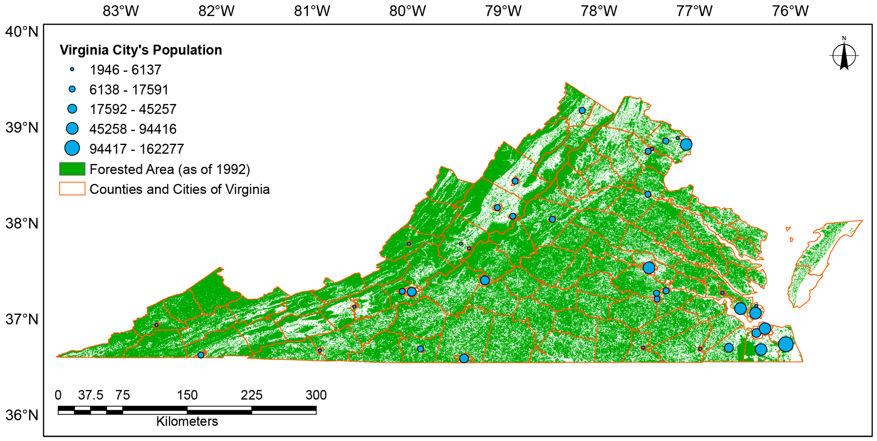
Figure 2.
Display of all geocoded points for both datasets from which the validation dataset was sampled.
Figure 2.
Display of all geocoded points for both datasets from which the validation dataset was sampled.
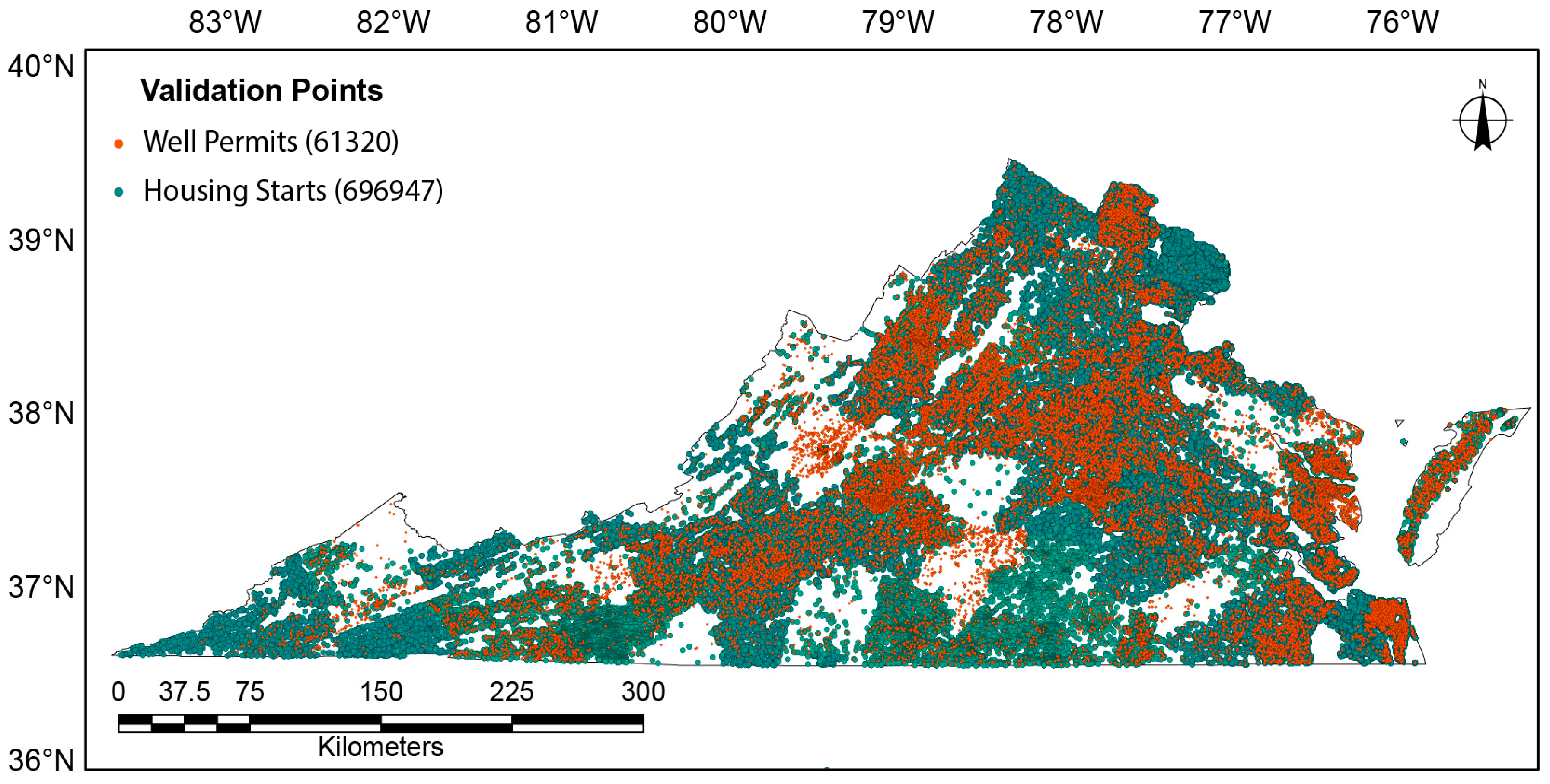
Figure 3.
Classes Development Disturbed and Non-Development Disturbed over time. Both were flagged as the low in 2003. Development Disturbed remains lower than Non-Development Disturbed through the remainder of the time series and is much more constant. These are two vector representations, but are not representative of all possible vectors.
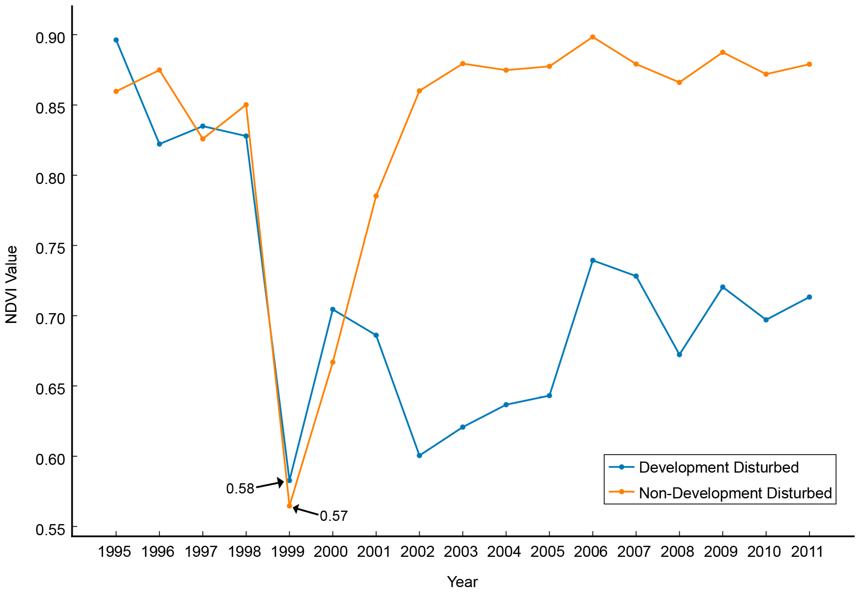
Figure 4.
The six predictor variable used in D3. The two selected predictor variables from CART® (Recovery Maximum and Recovery Slope) are labeled by violet text (or grey text printed in B&W).
Figure 4.
The six predictor variable used in D3. The two selected predictor variables from CART® (Recovery Maximum and Recovery Slope) are labeled by violet text (or grey text printed in B&W).
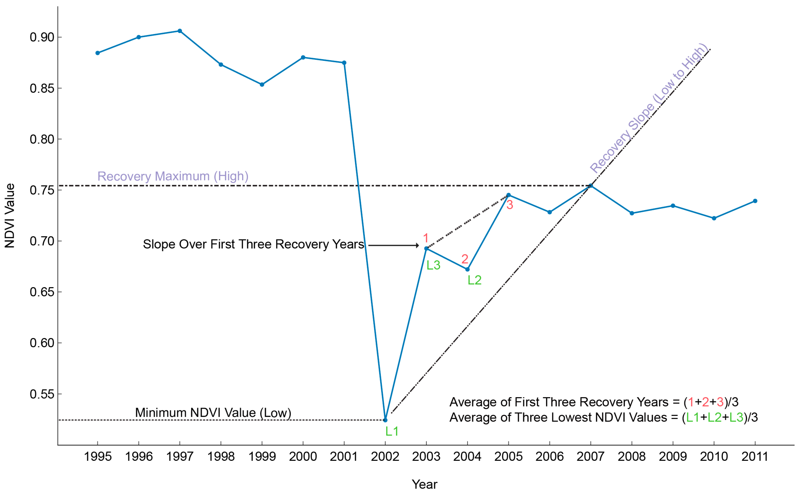
Figure 5.
Process with which points were selected for the accuracy assessments.

Figure 6.
Resulting CART® Tree from Salford Predictive Modeler v6.6. Cases in boxes shaded blue were classified as Development Disturbed while cases in the box shaded orange were classified as Non-Development Disturbed.
Figure 6.
Resulting CART® Tree from Salford Predictive Modeler v6.6. Cases in boxes shaded blue were classified as Development Disturbed while cases in the box shaded orange were classified as Non-Development Disturbed.
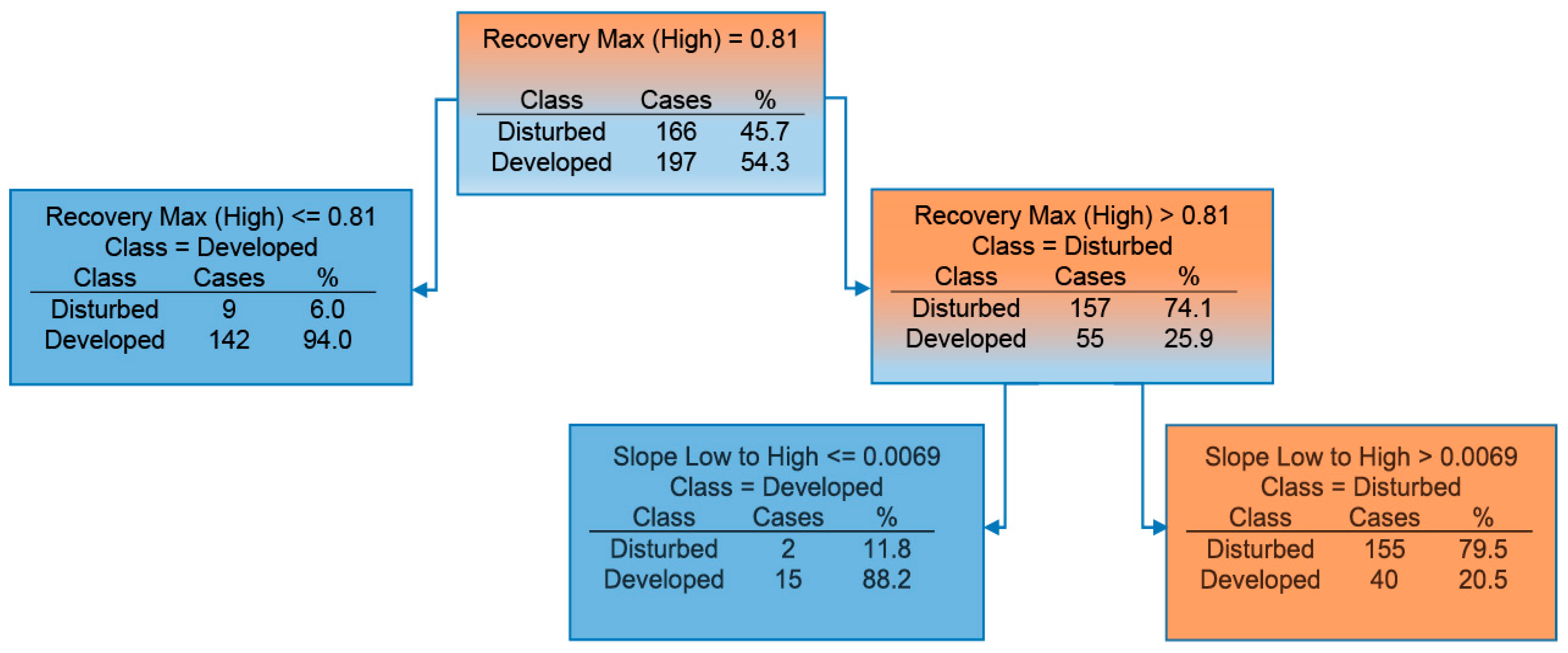
Figure 7.
Scatterplot (a) shows the first break in CART® using Recovery Maximum (high) as the splitter. All blue sample points/terminal nodes are Development Disturbed, all orange sample points/terminal nodes are Non-Development Disturbed. The points with Recovery Maximum (high) <0.81 are classified as Development Disturbed (terminal node); the nonterminal node points above that threshold are displayed in scatterplot (b). Using the splitter Recovery Slope (low to high) results in the final two terminal nodes. Boxplot (c) shows the first split while boxplot (d) shows the second split.

Figure 8.
An example of where NLCD detects change once the five-pixel threshold is met compared to the D3-based CART model, which is not constrained by that limitation.
Figure 8.
An example of where NLCD detects change once the five-pixel threshold is met compared to the D3-based CART model, which is not constrained by that limitation.

Table 1.
Classes used derived from NLCD Change Product (2001 to 2011) to derive an error matrix.
| FROM | Deciduous Forest | Evergreen Forest | Mixed Forest | Woody Wetlands |
|---|---|---|---|---|
| TO | Developed-Open Space | Developed-Open Space | Developed-Open Space | Developed-Open Space |
| Developed-Low Intensity | Developed-Low Intensity | Developed-Low Intensity | Developed-Low Intensity | |
| Developed-Medium Intensity | Developed-Medium Intensity | Developed-Medium Intensity | Developed-Medium Intensity | |
| Developed-High Intensity | Developed-High Intensity | Developed-High Intensity | Developed-High Intensity |
Table 2.
Error matrix from the D3-based CART model.
| Reference Data | |||||
|---|---|---|---|---|---|
| Combined Forest | Development Disturbed | Total | UA (%) | ||
| Classified Data | Combined Forest | 153 | 28 | 181 | 84.5 |
| Development Disturbed | 33 | 60 | 93 | 64.5 | |
| Total | 186 | 88 | |||
| PA (%) | 82.3 | 68.2 | |||
Table 3.
Error matrix from NLCD Change Product map.
| Reference Data | |||||
|---|---|---|---|---|---|
| Combined Forest | Development Disturbed | Total | UA (%) | ||
| Classified Data | Combined Forest | 186 | 88 | 274 | 67.9 |
| Development Disturbed | 0 | 0 | 0 | 0 | |
| Total | 186 | 88 | |||
| PA (%) | 100 | 0 | |||
© 2018 by the authors. Licensee MDPI, Basel, Switzerland. This article is an open access article distributed under the terms and conditions of the Creative Commons Attribution (CC BY) license (http://creativecommons.org/licenses/by/4.0/).
Share and Cite
MDPI and ACS Style
House, M.N.; Wynne, R.H. Identifying Forest Impacted by Development in the Commonwealth of Virginia through the Use of Landsat and Known Change Indicators. Remote Sens. 2018, 10, 135. https://doi.org/10.3390/rs10010135
AMA Style
House MN, Wynne RH. Identifying Forest Impacted by Development in the Commonwealth of Virginia through the Use of Landsat and Known Change Indicators. Remote Sensing. 2018; 10(1):135. https://doi.org/10.3390/rs10010135
Chicago/Turabian StyleHouse, Matthew N., and Randolph H. Wynne. 2018. "Identifying Forest Impacted by Development in the Commonwealth of Virginia through the Use of Landsat and Known Change Indicators" Remote Sensing 10, no. 1: 135. https://doi.org/10.3390/rs10010135
Note that from the first issue of 2016, this journal uses article numbers instead of page numbers. See further details here.