A Satellite-Based Model for Simulating Ecosystem Respiration in the Tibetan and Inner Mongolian Grasslands

Abstract

It is important to accurately evaluate ecosystem respiration (RE) in the alpine grasslands of the Tibetan Plateau and the temperate grasslands of the Inner Mongolian Plateau, as it serves as a sensitivity indicator of regional and global carbon cycles. Here, we combined flux measurements taken between 2003 and 2013 from 16 grassland sites across northern China and the corresponding MODIS land surface temperature (LST), enhanced vegetation index (EVI), and land surface water index (LSWI) to build a satellite-based model to estimate RE at a regional scale. First, the dependencies of both spatial and temporal variations of RE on these biotic and climatic factors were examined explicitly. We found that plant productivity and moisture, but not temperature, can best explain the spatial pattern of RE in northern China’s grasslands; while temperature plays a major role in regulating the temporal variability of RE in the alpine grasslands, and moisture is equally as important as temperature in the temperate grasslands. However, the moisture effect on RE and the explicit representation of spatial variation process are often lacking in most of the existing satellite-based RE models. On this basis, we developed a model by comprehensively considering moisture, temperature, and productivity effects on both temporal and spatial processes of RE, and then, we evaluated the model performance. Our results showed that the model well explained the observed RE in both the alpine (R² = 0.79, RMSE = 0.77 g C m⁻² day⁻¹) and temperate grasslands (R² = 0.75, RMSE = 0.60 g C m⁻² day⁻¹). The inclusion of the LSWI as the water-limiting factor substantially improved the model performance in arid and semi-arid ecosystems, and the spatialized basal respiration rate as an indicator for spatial variation largely determined the regional pattern of RE. Finally, the model accurately reproduced the seasonal and inter-annual variations and spatial variability of RE, and it avoided overestimating RE in water-limited regions compared to the popular process-based model. These findings provide a better understanding of the biotic and climatic controls over spatiotemporal patterns of RE for two typical grasslands and a new alternative up-scaling method for large-scale RE evaluation in grassland ecosystems.

1. Introduction

Grasslands are one of the most widespread vegetation types and store one-fifth of the total global carbon in its vegetation and soil [1,2]; thus, they play an important role in the global carbon cycle. The extensive grasslands in China make up ~10% of the total area of grasslands in the world and have been estimated to store 9–15% of the total carbon held in the grasslands worldwide [3]. Northern China’s grasslands located in the Tibetan Plateau and Inner Mongolian Plateau, in particular, constitute the majority (more than 70%) of the grasslands in China and represent two significant grassland types worldwide (i.e., alpine and temperate grasslands) [4]. Moreover, they are sensitive to climate changes due to their unique plateau topography, the extreme cold, arid and semi-arid ecological environment and the high soil carbon density [5,6,7]. Therefore, a better understanding of the carbon cycle in northern China’s grasslands is necessary for it to serve as a sensitivity indicator of regional and global carbon cycles.

Ecosystem respiration (RE) is an important outflow component of ecosystem carbon cycle and represents the second largest carbon exchanges between terrestrial ecosystems and the atmosphere [8]. However, as the result of the complex interactions among physical, chemical, and biological processes, RE varies greatly at different temporal and spatial scales [9]. Extensive studies at regional or global scales suggest that RE estimates still remains a large uncertainty [10]. Therefore, it is particularly essential but challenging to accurately evaluate the regional RE in northern China’s grasslands for a quantitative assessment of the terrestrial ecosystem carbon budget and its response to future climate changes.

Generally, modeling is the commonly adopted method for inferring RE at a large scale. Remote-sensing models, with relatively simple model structures and high spatiotemporal resolutions, provide promising tools for monitoring regional RE. Currently, with the development of fine-scale remote-sensing technology and long-term regional and global FLUXNET observations, extensive studies have revealed the robust statistical and physiologically meaningful relationships between RE and satellite products, e.g., the land surface temperature (LST) [11,12,13] and vegetation index (VI) [14,15,16]. Based on this information, many semi-empirical satellite-based models were developed and well validated at the plot scale [13,16,17,18,19]. However, RE at large scale involves complex spatial and temporal variation processes [20]. Few satellite-based models have an explicit representation of the spatial process of RE. Specifically, the basal respiration rate, an important parameter in RE models to describe the location-specific respiration rate, is usually set as a constant parameter, which introduces considerable error in the simulated spatial variability of RE [8,20,21]. Therefore, it is critical to identify the controlling mechanism involved in the spatial variations of RE with more comprehensive data, not just in the temporal variations, thus serving as a valuable basis to better understand patterns of RE at regional scale and to scale-up from specific sites to vegetation biomes. In addition, both climatic and biotic controls over RE should be considered comprehensively in RE simulation [22,23]. In satellite based models, RE has often been linked to temperature or plant productively solely. Some studies advanced RE estimates by accounting for the combined two effects of temperature and plant productivity [13,15]. The moisture limitation on RE is often lacking in most of the current satellite-based respiration models, leading to a potential underestimation of drought effects on respiration (e.g., [19,24]). However, grasslands are one of the most sensitive ecosystems to the alteration of water regimes [25]. Water stress was found to have a strong influence on northern China’s grasslands, especially in southwestern Inner Mongolia and northwestern Tibet [26]. Recently, some satellite-based models gradually began incorporating the moisture effect on RE, but it still depends which satellite product and form are selected to represent the moisture factor and the response process of RE to moisture. For instance, a linear equation of an indirect water indicator (diurnal LST difference, LST_diff) was utilized in the RECO model during the dry season for water-limited biomes, which were mostly concentrated in the Mediterranean climate region without a temperature limitation [27]; thus, its utility in northern China’s grasslands still needs to be validated. Root-zone soil moisture derived from the Advanced Microwave Scanning Radiometer-Eos was adopted in a soil respiration (Rs) model in the Midwest USA, and it yielded a lower explanation capacity for seasonal variation of Rs than the surface soil moisture under extreme moisture regimes [28]. Currently, increasing attention is being given to the moisture effect on RE [29,30], as most climate change scenario analyses have predicted that the frequency and severity of drought will increase in most biomes across the world [31]. It is practical to develop a satellite-based RE model that integrates temperature, plant productivity, and moisture effects together in both temporal and spatial processes, to yield reliable simulations of regional RE for northern China’s grasslands.

This study was based on 57 site-year flux-tower data and remote-sensing data from northern China’s grasslands. The major objectives of this study were threefold: (i) to quantify the relationships of climatic and biotic factors and the spatial and temporal variability of RE in the Tibetan alpine grasslands and the Inner Mongolian temperate grasslands; (ii) to develop a high-resolution satellite-based model for simulating RE at regional scale on the basis of comprehensive consideration of vegetation productivity, temperature, and moisture; and (iii) to assess the model performance in terms of the temporal dynamics as well as the spatial pattern simulation of RE in northern China’s grasslands.

2. Materials and Methods

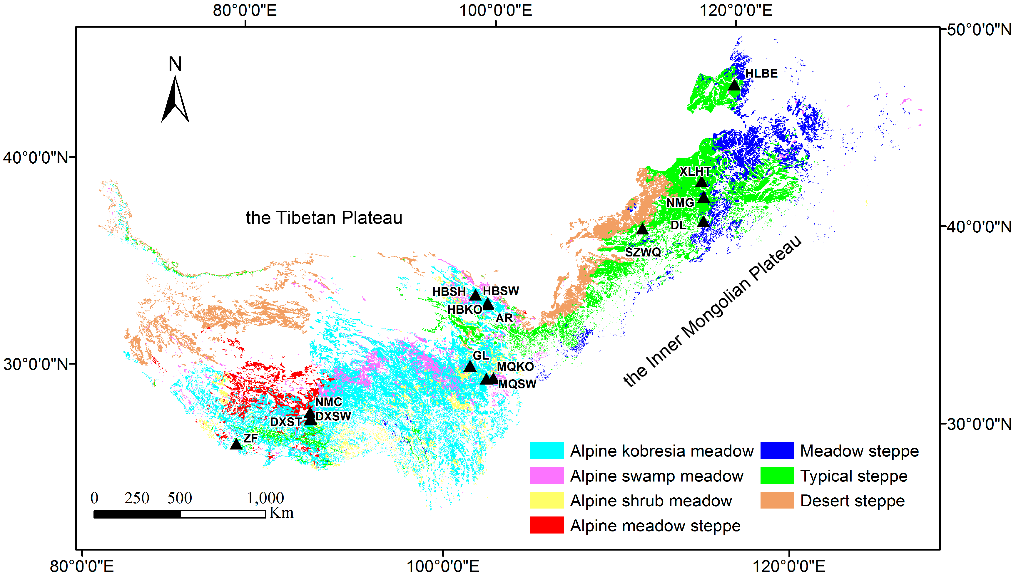
2.1. Study Area

This study was conducted in the alpine grasslands on the Tibetan Plateau and the temperate grasslands on the Inner Mongolian Plateau. The Tibetan region is in the alpine climate zone, where temperature appears as the controlling factor for the grassland ecosystems. With an average elevation of ca. 4000 m, the mean annual air temperature on the plateau ranges between −5.75 and 2.57 °C, and the mean annual precipitation varies from 200 to 600 mm. The alpine meadow covers more than half of the plateau, representing not only a typical ecosystem in central Asia alpine environment but also a unique ecosystem within the alpine regions of the world [32]. Located in the arid and semi-arid zone, the grassland ecosystems in the Inner Mongolian region are mainly limited by moisture. With an average elevation ca. 1000 m, the mean annual temperature in this area varies between 3 and 6 °C, and the mean annual precipitation ranges from 200 to 350 mm. The temperate grasslands are a typical vegetation type under the temperate continental climate and they represent an important component of the Eurasian grasslands [33]. According to the Atlas of China’s Grassland Resources (1:1,000,000), we fully considered the spatial representativeness of the flux-tower sites collected for this research and focused on three types: (i) alpine meadow; (ii) alpine meadow steppe (AS); and (iii) temperate steppe. The alpine meadow was further subdivided into three types: (1) alpine Kobresia meadow (KO); (2) alpine shrub meadow (SH); and (3) alpine swamp meadow (SW); the temperate steppe was also subdivided into three types: (1) meadow steppe (MS); (2) typical steppe (TS); (3) and desert steppe (DS). The distribution of these vegetation functional types (PFTs) as well as the typical grassland flux-tower sites is shown in Figure 1.

2.2. Data

2.2.1. Flux-Tower Data

A total of 57 site-year data from 16 grassland sites during 2003–2013 were retrieved from the ChinaFLUX and the Coordinated Observations and Integrated Research over Arid and Semi-Arid China (COIAS) databases, including 43 site-years from 11 sites on the Tibetan Plateau and 14 site-years from 5 sites on the Inner Mongolia Plateau (

Table 1. Main characteristics of the 16 flux-tower sites over China’s grasslands.

Grassland Type	Site Name	Location	Elevation (m)	Canopy Height (m)	Tower Height (m)	Operation Period
Alpine shrub meadow	HBSH	37.67°N 101.33°E	3293	0.6–0.7	2.2	2003–2008, 2010–2012
Alpine Kobresia meadow	HBKO	37.61°N 101.31°E	3148	0.2–0.3	2.2	2003–2005, 2009, 2012
	GL	34.35°N 100.56°E	3980	0.2–0.3	2.2	2007, 2010–2011, 2013
	AR	38.04°N 100.46°E	3033	0.2–0.3	3.15	2008–2010
	MQKO	33.88°N 102.15°E	3533	0.2–0.3	3.15	2009–2010
Alpine swamp meadow	HBSW	37.61°N 101.33°E	3160	0.2–0.5	2.2	2004–2008, 2010–2012
	DXSW	30.47°N 91.06°E	4286	0.2–0.5	2.1	2009–2010
	MQSW	33.76°N 101.68°E	3503	0.3–0.5	3.2	2010
Alpine meadow steppe	DXST	30.50°N 91.06°E	4333	<0.2	2.2	2004–2010
	ZF	28.36°N 86.95°E	4293	<0.2	3.1	2009
	NMC	30.77°N 90.96°E	4730	<0.2	3.1	2009
Typical steppe	NMG	43.53°N 116.67°E	1200	0.2–0.3	4	2004–2008, 2010, 2012
	DL	42.05°N 116.28°E	1324	0.3–0.5	5	2010–2011
	XLHT	44.13°N 116.32°E	1187	0.1–0.3	5	2010–2011
Desert steppe	SZWQ	41.8°N 111.9°E	1438	0.1–0.2	3	2011–2012
Meadow steppe	HLBE	49.06°N 119.4°E	628	0.3–0.5	3	2012

). The observed eddy-covariance data were processed through a three-dimensional coordinate rotation, WPL (Webb-Pearman-Leuning) correction, and invalid data exclusion [34]. Subsequently, the missing nighttime RE and daytime RE data were calculated using the Lloyd-Taylor equation based on net ecosystem exchange (NEE) observations during the nighttime [35]. The entire procedure was completed using the ChinaFLUX CO₂ data processing system [36]. The half-hourly flux data was summed to obtain daily values, and the site-years with more than 30% of the daily RE missing were eliminated. To comply with the temporal scale of the Moderate Resolution Imaging Spectroradiometer (MODIS) 8-day composite imagery, the processed daily RE were averaged within the same periods.

2.2.2. Remote-Sensing Data

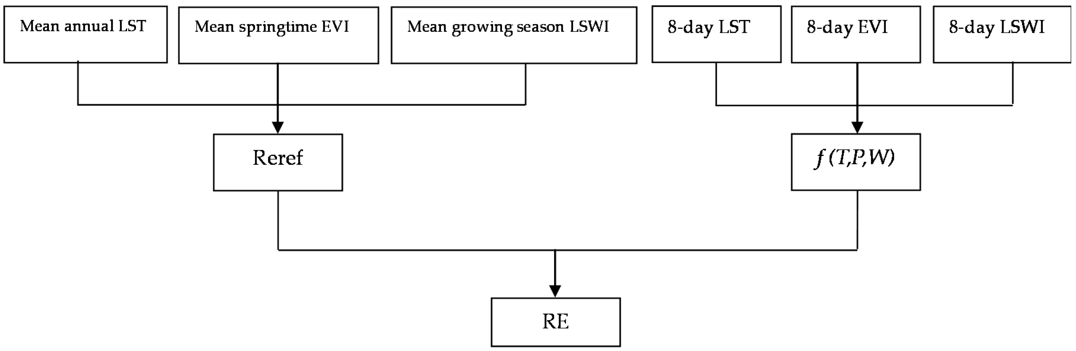
At the site scale, the MODIS products of the LST, enhanced vegetation index (EVI), and land surface water index (LSWI) at each site-year (2003–2013) were downloaded from the University of Oklahoma Data Center (http://www.eomf.ou.edu/visualization/manual/), based on the pixels where the flux towers located, to match up with the flux data for model parametrization.

At the spatial scale, the 8-day (best observation in 8 days) MODIS land surface reflectance datasets (MOD09A1, Level 3, Collection 5) during 2001–2010 were downloaded from NASA Land Processes Distributed Active Archive Center (https://lpdaac.usgs.gov/) to generate the spatial EVI and LSWI data using Equations (1) and (2), as model drivers in regional simulation.

$$EVI=G\times ({\rho }_{nir}-{\rho }_{red})/({\rho }_{nir}+(C_1\times {\rho }_{red}-C_2\times {\rho }_{blue})+L),$$

(1)

$$LSWI=({\rho }_{nir}-{\rho }_{swir}) / ({\rho }_{nir}+{\rho }_{swir}),$$

(2)

where ${\rho }_{nir}$, ${\rho }_{red}$, ${\rho }_{blue}$, and ${\rho }_{swir}$ represent the reflectance of near infrared bands (NIR, 841–875 nm), red bands (620–670 nm), blue bands (459–478 nm), and short wave infrared bands (SWIR, 1628–1652 nm), respectively. The coefficients G, C₁, C₂ and L used in the EVI algorithm are 2.5, 6, 7.5 and 1, respectively [37].

The MOD11A2 and MYD11A2 products (Level 3, Collection 5), which are 8-day average values of cloud free observations, were also downloaded from the LP DAAC data pool to obtain the spatial daytime LST and nighttime LST data, respectively. The spatial resolution of EVI and LSWI is 500 m, and that of LST is 1 km. For the regional application in China’s grasslands, the extracted EVI and LSWI were resampled to a 1-km resolution. The temporal resolution of these products is 8-day, which ensures a better data quality as selected on the basis of the absence of clouds or aerosol, etc., and is confirmed by extensive RE modeling research to be able to robustly capture the seasonal variation of RE [24,27,28]. Additionally, to further reduce the effect of cloud and to capture the seasonality of EVI, the original time series were smoothed using the double logistic curve fit in the TIMESAT software (Lund University, Lund, Sweden) [38].

2.3. Model

RE at the regional scale is a coupling result of complex spatial and temporal processes. The process of spatial variability refers to the basic trend of RE changing with the climate and substrate at a specific location, which is especially significant in regional simulations [39]; the process of temporal variability refers to the cyclical changes of RE induced by the seasonal dynamics of environmental factors and plant growth. A multiplication factor is usually used to express the interaction of the above two processes in an RE simulation [20,21,22,27]. Based on the remote-sensing model RECO [27] and the traditional climate-driven model T&P [20,22], we put forward a modified model of RE for grasslands by taking the effects of temperature, vegetation productivity, and moisture on both the spatial and temporal variability of RE into account and making full use of the high-resolution satellite data as the model drivers. To account for spatial and temporal variability separately, we partition RE into a site-specific reference respiration rate (Reref) and the remaining seasonal variation (f(T,P,W)), which is detrended for site characteristics (Equation (3)). The structure of the model is shown below (Figure 2).

$$RE=Reref\ast f (T, P, W),$$

(3)

2.3.1. Representation of Spatial Variability of RE

Reref is the site-specific respiration rate at the reference temperature (Tref). It is used to describe the difference in basal respiration between sites and years, thereby reflecting the spatial variability of RE [8]. Numerous studies have indicated that a spatially heterogeneous Reref results in a better estimation of RE at different sites [20,21,22,27]. The long-term spatial variation of RE or Reref is found to be mainly driven by the mean annual temperature [40,41,42], mean annual plant productivity [43,44], and mean annual moisture [45,46,47]. Thus, the functional description of Reref in this study is developed based on its dependencies on the temperature, productivity, and moisture factor (Figure 3). Since Reref becomes less suitable to capture site characteristics at higher Tref values [27], Tref was set as the mean springtime (DOY 96-144) temperature (i.e., 3 °C for the Tibetan alpine grasslands, and 7 °C for the Inner Mongolian temperate grasslands), and the Reref for each site-year was calculated as the mean respiration rate at the temperature approximate to Tref during the spring time. Finally, Reref is estimated in our model as follows:

$$Reref=p_1+p_2\ast {EVI}_{mean}+p_3\ast {LST}_{mean}+p_4\ast {LSWI}_{mean},$$

(4)

where EVI_mean is the mean annual springtime EVI, LST_mean is the mean annual daytime LST (LST_d), LSWI_mean is the mean annual growing season LSWI (DOY 136-272), and p₁ to p₄ are parameters to be inferred herein. Figure 3 displays the Reref dependencies on EVI_mean, LST_mean and LSWI_mean.

2.3.2. Representation of Temporal Variability of RE

The seasonal dynamics of RE are reflected by $f(T,P,W)$, which is mainly controlled by the temporal variability of temperature [48,49], vegetation productivity [43,50], and water [20,21,22,40]. Especially in the arid and semi-arid ecosystems, water is the main limiting factor of the seasonality of RE [51,52]. The values of f(T,P,W) are obtained by calculating the ratio of the observed RE from the flux tower and the site-specific Reref partitioned from the observed RE. Figure 4 displays the $f(T,P,W)$ dependencies on the temporal variation of EVI, LST and LSWI. The form of $f(LST,EVI)$ scalar was based on the LST-driven Lloyd-Taylor equation [48] and EVI-driven linear equation, while the form of fw scalar was derived from a Michaelis-Menten equation firstly proposed by Raich et al. [53]. During the growing season, we calculate the $f(T,P,W)$ as follows:

$$f(T,P,W)=f(LST,EVI)\ast f_W,$$

(5)

$$f(LST,EVI)=p_5\ast \exp (E_0\ast (\frac{1}{Tref-T_0}-\frac{1}{{LST}_n-T_0}))+p_6\ast {EVI}_{std}+p_7,$$

(6)

$$f_W=\frac{(0.5+LSWI)}{k+(0.5+LSWI)},$$

(7)

where LST_n is nighttime LST, EVI_std is the standardized EVI (8-day EVI divided by EVI_mean), p₅ to p₇ are the parameters to be sought, E₀ is the activation energy, T₀ is the minimum temperature for respiration, which is set to 227.13 k (−46.02 °C) as in the original Lloyd-Taylor model, k is the half-saturation constant of the hyperbolic relationship, and 0.5 is an empirically given value to maintain the numerator/denominator of fw > 0.

During the non-growing season, temperature, but not water, becomes the main limiting factor for RE in northern China’s grasslands [24]. In addition, the surface covered by ice and snow in the non-growing season has a strong absorption of the shortwave infrared band that causes LSWI to increase sharply; thus, it cannot reflect the actual water content in the winter [54]. Therefore, the fw scalar is only considered for the growing season (Equation (5)). During the non-growing season, we calculate the temporal variability of RE as follows:

$$f(T,P,W)=f(LST,EVI) ,$$

(8)

The different periods of MODIS indices (i.e., the mean springtime of EVI, the mean annual of LST_d in Reref, and LST_n in $f(T,P,W)$) used here have already been selected by Jägermeyr et al. [27] as the best index for fitting the relationship with RE. LSWI, selected by us as the model driver, is a more direct proxy for moisture than LST_diff, which was used in RECO but had no significant relation with the temporal dynamics of RE in our study (R² < 0.2, p > 0.05); in addition, land surface moisture was found to have greater influence on RE than deep soil water [20,28], which is especially instrumental in northern China’s grasslands with the large number of roots distributed in the soil surface [55]. Therefore, all these drivers appear to be chosen empirically but are based on the physiological dependencies of RE, thereby ensuring reliable estimates from our model.

2.4. Model Parameterization and Validation

The two components, i.e. Reref for each site and year and the remaining seasonal variation f(T,P,W) partitioned from the overserved RE, were used to optimize parameters for Equations (4) and (5) separately to better constrain each component of the model. The nonlinear least-squares curve fitting method was utilized to estimate the model parameters. In addition to joint-sites estimation for the two grasslands in two regions, the leave-one-out cross validation method was employed to test the validity of the joint estimation of parameters (i.e., one subtype was excluded at a time, and the data for all other subtypes were used to estimate the parameters for each grassland type). The coefficient of determination (R²) and root mean square error (RMSE) were chosen to assess the model performance. Regional-scale application is based on PFT-specific parameters retrieved from the entire site-data of alpine grasslands and temperate grasslands to assure most robust parameters.

To further verify the model improvement by incorporating the moisture effect on both spatial and temporal variability, the LSWI_mean in Reref and fw in f(T,P,W) were removed, respectively, to test the accuracy of the model. In addition, we also compare some other semi-empirical or process-based models to assess the ability of our model. Specifically, for the RE estimation at a site scale, we chose the two original models that our model was based on, namely T&P [22] and RECO [27]; for the RE estimation at a regional scale, an independent regional RE product simulated by a mainstream dynamic global vegetation model CLM4CN, derived from Piao et al. [56], was applied.

3. Results

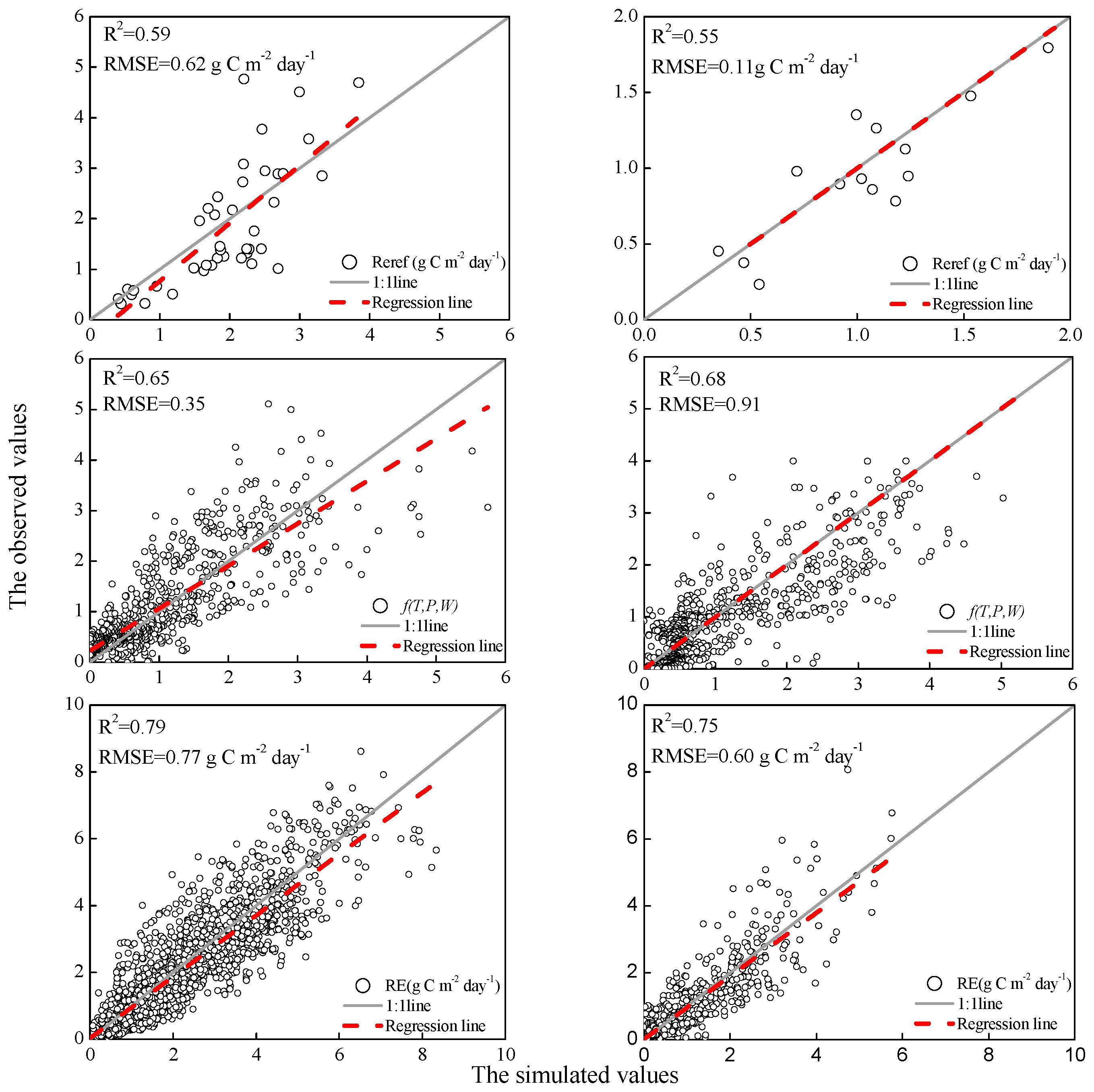
3.1. Quantitative Relationships between RE and Biotic and Climatic Factors

The observed RE values were partitioned into Reref and f(T,P,W) to account for the spatial and temporal variability of RE separately. The quantitative relationships between these two components and the climatic and biotic factors provided a clear physiological basis for the development of the model.

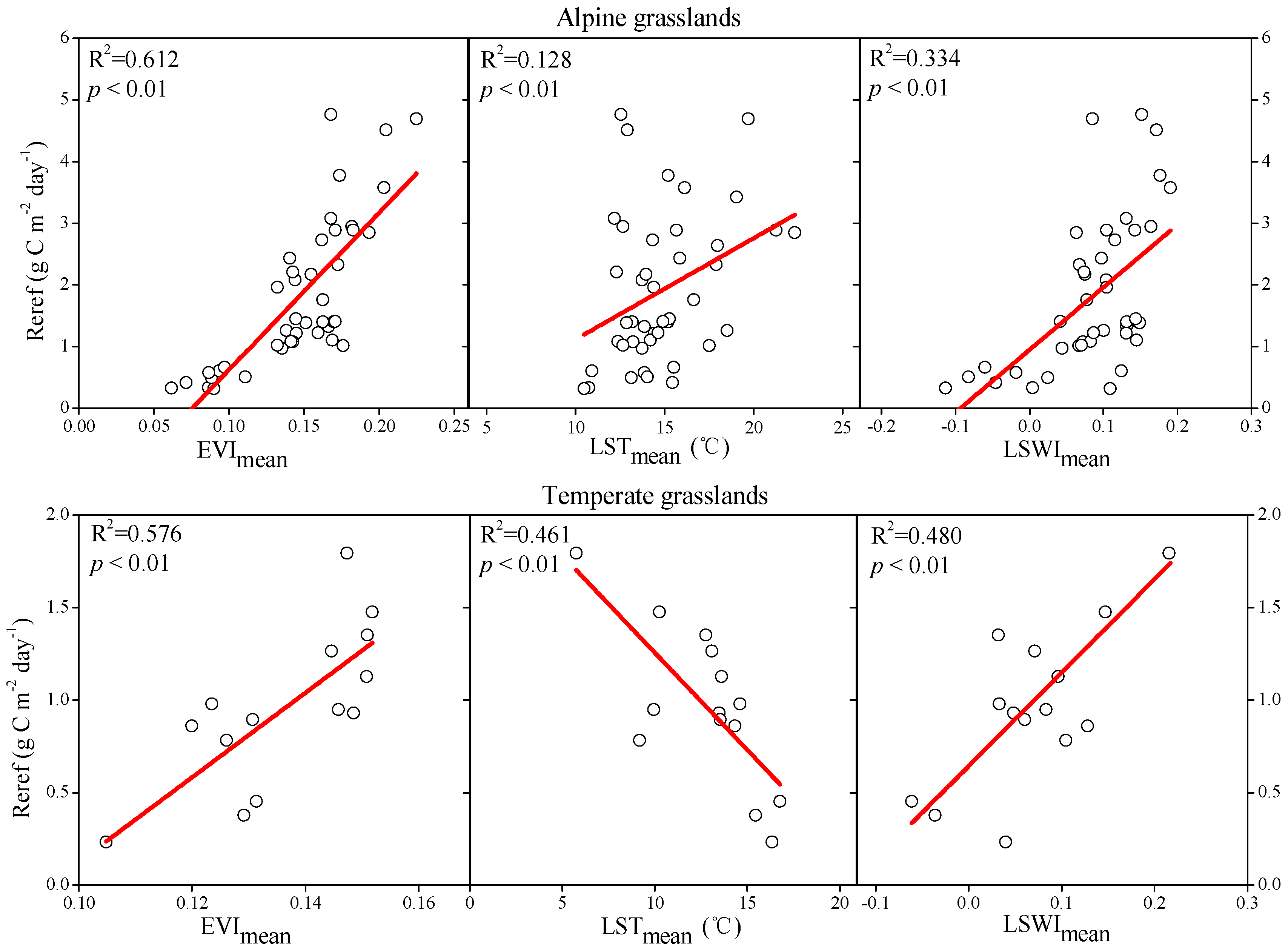
3.1.1. Quantitative Relationships between Reref and Biotic and Climatic Factors

Multiple regression analyses between Reref and the remote-sensing data show that Reref has a significant dependence on EVI_mean, LST_mean and LSWI_mean, which can be approximated linearly (Figure 3). The variation of Reref in the Tibetan alpine grasslands is primarily attributed to the change in vegetation productivity (EVI_mean, R² = 0.612) and to the water regime (LSWI_mean, R² = 0.334). Temperature plays a negligible role in the Reref (LST_mean, R² = 0.128). Similarly, productivity (R² = 0.576) and moisture (R² = 0.480) tend to be more important than temperature (R² = 0.461) for Reref in the temperate grasslands of Inner Mongolia. However, the temperature limitation among the temperate grassland sites is characterized by a negative slope.

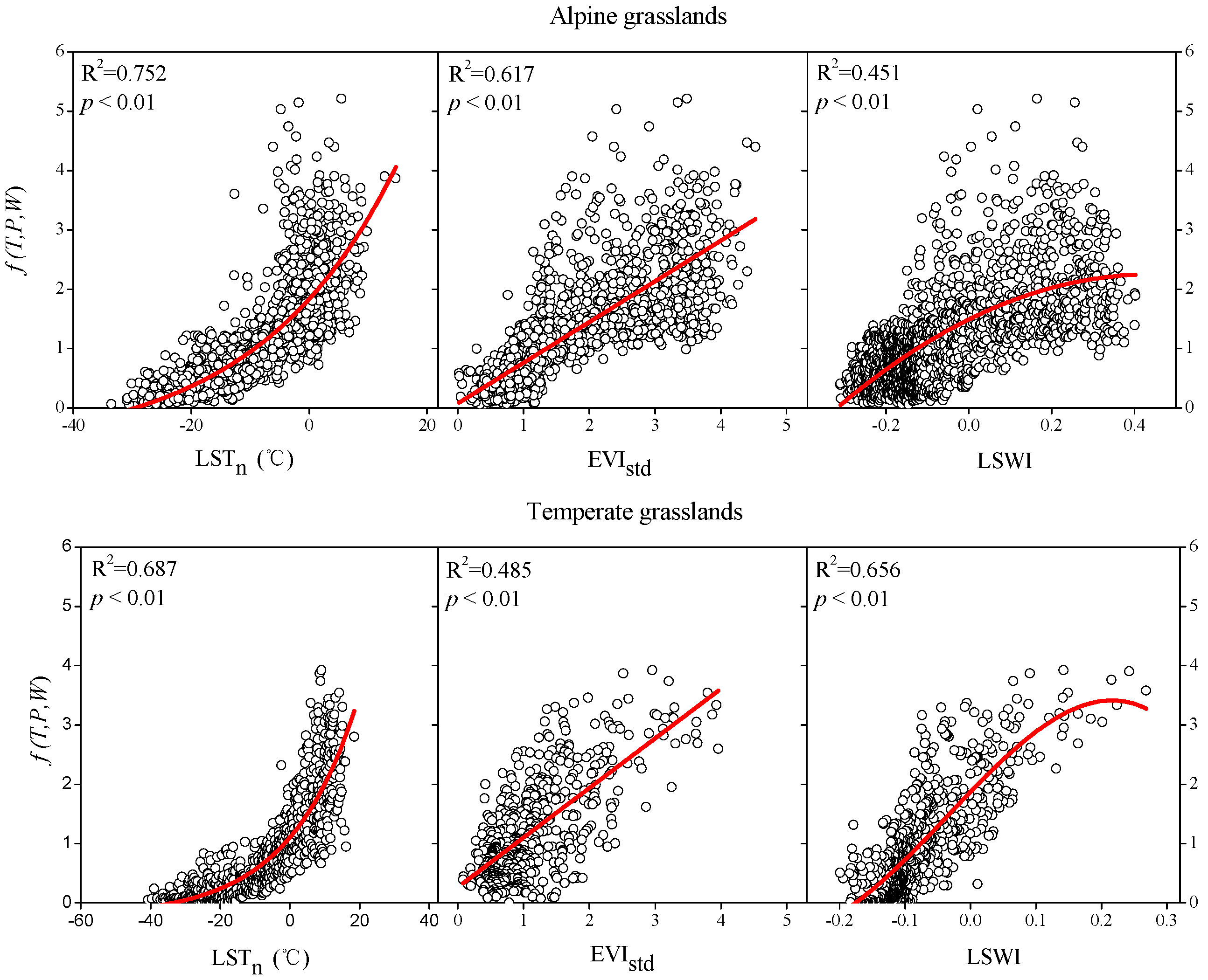
3.1.2. Quantitative Relationships between $f(T,P,W)$ and Biotic and Climatic Factors

The regression analyses between $f(T,P,W)$ and the remote-sensing indexes (Figure 4) indicate that the temporal variability of RE has a strong exponential dependency on temperature, which could be described using the LST_n-driven Lloyd-Taylor equation. RE still has a significant linear response to the seasonal dynamics of EVI, which is decided by the behind mechanism that growth respiration supplies energy at the cost of consuming some photosynthate, causing the RE to be approximate to a constant fraction of plant productivity [57,58]. In terms of the response to temporal variation of LSWI, RE is almost linearly related to LSWI firstly (when LSWI < 0.1) and then it reaches saturation during the final stage in the Inner Mongolian region with a relatively low soil water content, whereas in the Tibetan region with a relatively high soil water content, the response of RE to LSWI follows a gradual saturation. The responses of RE to moisture under the two different water regimes both agree well with the typical Michaelis-Menten curve.

The temporal variation of RE in the alpine grasslands of the Tibetan Plateau is mainly correlated to temperature (LST_n, R² = 0.752), followed by plant productivity (EVI_std, R² = 0.617), while water (LSWI, R² = 0.451) plays a minor role in regulating the temporal dynamics of RE in this temperature-limited region (Figure 4). In contrast, water exerts a strong influence (LSWI, R² = 0.656) on the temporal variability of RE in the temperate grasslands of Inner Mongolia, which is comparable with the determinant factor (LST_n, R² = 0.687), while plant productivity exerts a relatively weak impact (EVI_std, R² = 0.485).

3.2. Model Parameterization and Validation

Based on the quantitative dependencies of spatiotemporal variability in RE to these biotic and environmental factors, we developed a semi-empirical RE model described in 2.3. The long-term flux tower-observed RE was used for parameter estimation and validation. Detailed parameter values for Reref and $f(T,P,W)$ in the two grasslands are presented in

Table 2. Parameter estimation of Reref and f(T,P,W) for two grassland types in two regions.

	Grassland Type	Alpine Grasslands		Temperate Grasslands
Reref	p1	−2.646 ± 0.456		−0.019 ± 0.023
	p2	15.100 ± 2.062		8.347 ± 1.068
	p3	0.173 ± 0.024		−0.029 ± 0.009
	p4	18.828 ± 0.939		3.952 ± 0.322
f(T,P,W)	p5	1.787 ± 0.081	(1.421 ± 0.136) *	0.658 ± 0.119	(0.941 ± 0.147) *
	E0	279.764 ± 53.87	(164.507 ± 31.874) *	166.327 ± 12.402	(154.305 ± 18.729) *
	p6	0.250 ± 0.024	(0.193 ± 0.046) *	0.944 ± 0.039	(0.085 ± 0.061) *
	p7	0.094 ± 0.039	(0.108 ± 0.046) *	−0.363 ± 0.081	(0.190 ± 0.050) *
	k	0.021 ± 0.064		0.207 ± 0.0.082

* Among the parameters for f(T,P,W), the values inside the parentheses are for the non-growing season, while the others are for the growing season.

. These parameters are mostly empirical coefficients varying with the vegetation types and structures, site conditions, and histories. One of the parameters for Reref, for example, p₃, has the opposite sign for the temperate grasslands (negative) relative to the alpine grasslands (positive). This phenomenon implies a negative correlation between the spatial variation of RE and mean annual temperature in Inner Mongolia. Among the parameters for f(T,P,W), the activation energy E₀ and the half saturation constant k are two key parameters that have a special physiological implication. In the alpine grasslands, E₀ has a higher value than the temperate grasslands. This result accurately reflects the increasing temperature sensitivity with the decreasing temperature. Regarding the half saturation constant, k, the value is higher (0.207) in the temperate grasslands than the alpine grasslands (0.021). The drier ecosystem has a higher half saturation point, accurately characterizing the different responses of RE to moisture among the alpine and the arid and semi-arid regions.

The model parameter estimation reveals that approximately 77.8% and 74.9% of the variation in the observed RE across the alpine and temperate grasslands, respectively, could be explained by this model, albeit with a small bias (Figure 5;

Table 3. Joint-sites estimation and leave-one-out cross validation for each vegetation type.

Vegetation Type	Types of Parameter Estimation	Types of Cross-Validation	R2	RMSE	p Value
Alpine Grasslands	SH_SW_ST	KO	0.844	0.841	<0.01
	KO_SW_ST	SH	0.756	1.047	<0.01
	KO_SH_ST	SW	0.917	0.927	<0.01
	KO_SH_SW	ST	0.784	1.544	<0.01
	Joint-sites (AR_GL_HBKO_GL)	/	0.778	0.774	<0.01
Temperate Grasslands	TS_DS	MS	0.803	0.405	<0.01
	MS_DS	TS	0.575	0.919	<0.01
	TS_MS	DS	0.643	1.021	<0.01
	Joint-sites (TS_MS_DS)	/	0.749	0.605	<0.01

, joint-sites). Specifically, the model could explain more than 55% of the spatial variability of RE (Reref) in the two regions. The simulation error in the Tibetan alpine grasslands (RMSE = 0.62 g C m⁻² day⁻¹) is higher than that in the Inner Mongolian temperate grasslands (RMSE = 0.11 g C m⁻² day⁻¹). The temporal variability (f(T,P,W)) is generally explained to a greater degree (more than 65%) compared to the spatial variability, while the simulation error in the temperate grasslands (0.91 g C m⁻² day⁻¹) is higher than that in the alpine grasslands (0.35 g C m⁻² day⁻¹). The cross-validation among subtypes in the alpine and temperate grasslands shows that approximately 75.6–91.7% and 57.5–80.3%, respectively, of the variation in the observed RE could be predicted by the model, with the values of RMSE ranging from 0.841 to 1.544 g C m⁻² day⁻¹ and 0.405–1.021 g C m⁻² day⁻¹ for the alpine and temperate grasslands, respectively (Table 3). Except for the typical steppe, where the parameters derived from the limited sites in the meadow steppe and desert steppe do not represent for the typical steppe well, the other vegetation types differ slightly in performances from the cross-validation and parameter estimation, which verifies the robustness of the parameterization results.

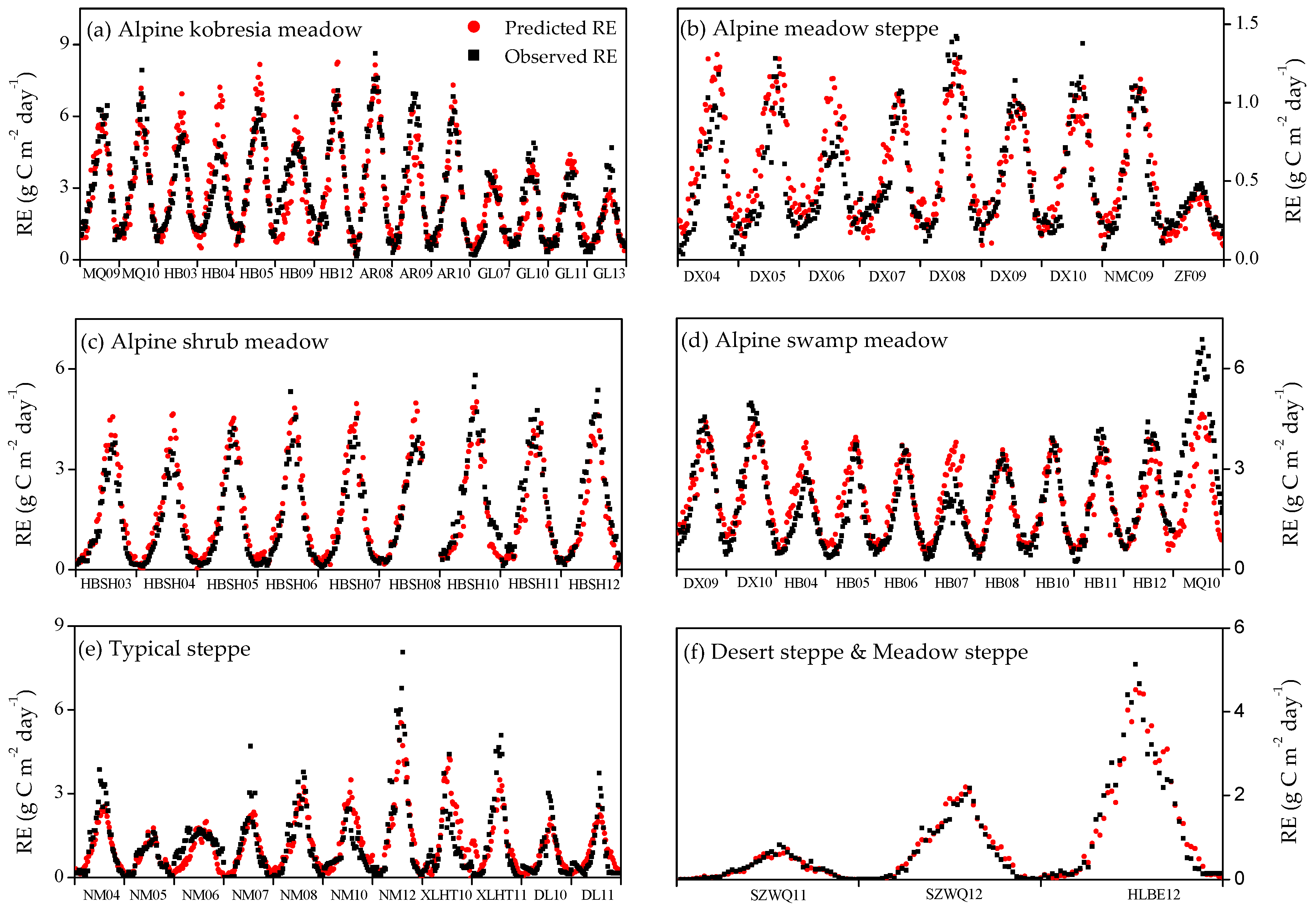
3.3. Model Simulation for Seasonal and Inter-Annual Dynamics of RE at the Site Scale

Using the model parameters in Table 2, we simulate time-series RE of all 57 site-years and then further compared them to the flux tower-observed RE for each vegetation subtype in the alpine and temperate grasslands. In most cases, the temporal variation of the RE is tracked robustly by our model (Figure 6). The agreement between the modeled and observed RE is the best for the desert steppe and meadow steppe (R² > 0.9), followed by the alpine shrub meadow (R² = 0.872), the alpine meadow steppe (R² = 0.805), the alpine Kobresia meadow (R² = 0.778), the typical steppe (R² = 0.743), and the alpine swamp meadow (R² = 0.715). Ground covered by water in the alpine swamp meadow would affect the spectral reflectance and further disturb the model drivers (EVI and LSWI), and this may be the main reason for the relatively low performance in this vegetation type.

The seasonal variation of RE in China’s grasslands could be described as a unimodal curve peaking in July or August. Across the seven vegetation types, the mean annual peak respiration rate ranges from 1.10 to 5.84 g C m⁻² day⁻¹. The highest value occurring in the alpine meadow or the meadow steppe is approximately four times higher than that of the alpine meadow steppe or the desert steppe. There are also significant inter-annual fluctuations in the RE at some sites; for instance, the observed RE decreased remarkably as precipitation decreased in 2011 in SZWQ (Figure 6f), 2005 and 2006 in NM (Figure 6e), and 2009 in HBKO (Figure 6a). In addition, our model could accurately reproduce the inter-annual dynamics of RE due to the variation in precipitation across years.

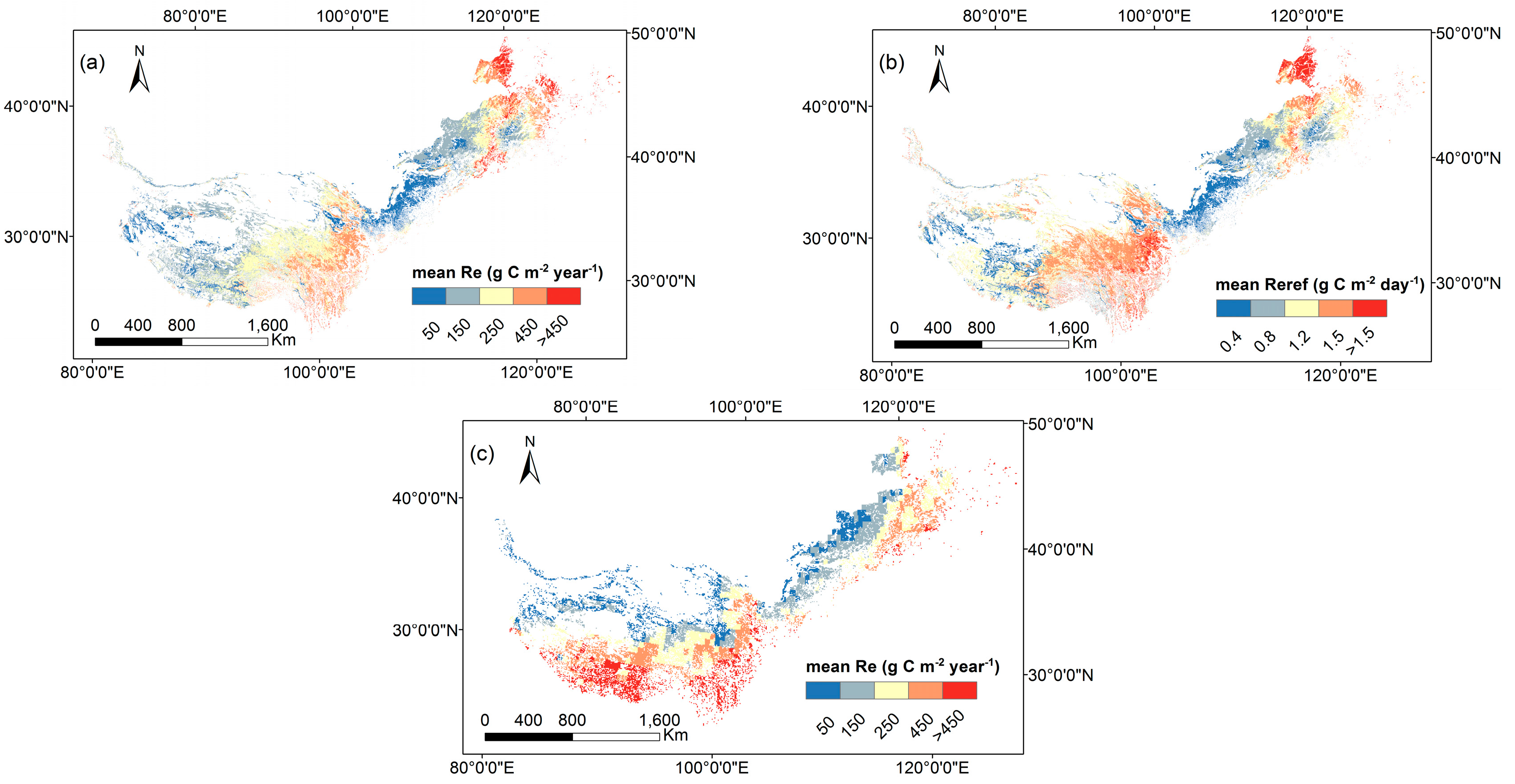
3.4. Model Simulation for Spatial Patterns of RE at the Regional Scale

Based on the parametrized RE model dependent on prescribed PFTs (alpine and temperate grasslands in Figure 1) and the spatial driver data of MODIS EVI, LST, and LSWI, the spatial distribution of the mean annual REs from 2001 to 2010 were obtained (Figure 7a). The predicted annual RE of China’s northern grasslands is 258.18 ± 12.07 g C m⁻² yr⁻¹ on average. For the alpine grasslands on the Tibetan Plateau, the alpine shrub meadow has the largest RE value (434.69 ± 8.83 g C m⁻² yr⁻¹), followed by the alpine swamp meadow (413.82 ± 8.21 g C m⁻² yr⁻¹), the alpine Kobresia meadow (368.64 ± 7.52 g C m⁻² yr⁻¹), and the alpine steppe meadow (146.57 ± 3.21 g C m⁻² yr⁻¹), exhibiting a clear decreasing gradient from the southeast to the northwest with increasing elevation across the Tibetan Plateau. For the Inner Mongolian Plateau, RE also shows a clear decreasing gradient from northeast to southwest. Specifically, the highest value of RE occurs in the meadow steppe (470.27 ± 39.24 g C m⁻² yr⁻¹) in the northeast, and the lowest value of RE occurs in the desert steppe in the southwest (144.91 ± 21.75 g C m⁻² yr⁻¹). The mean annual RE in the typical steppe is 193.6 ± 30.84 g C m⁻² yr⁻¹.

Reref appears to be a key component in this model in terms of quantifying the spatial variability of RE across sites. Nevertheless, the spatial patterns of Reref have rarely been investigated due to the lack of spatially explicit algorithms to allow the upscaling of Reref. Here, we took abiotic and biotic factors into consideration to parameterize Reref spatially and revealed that the mean annual Reref has a clear spatial heterogeneity among different vegetation types in northern China’s grasslands (Figure 7b), ranging from 0.22 g C m⁻² day⁻¹ in the desert steppe to 2.25 g C m⁻² day⁻¹ in the meadow steppe. In addition, the spatial distribution of Reref, to a large extent, determines the spatial pattern of the mean annul RE (Figure 7a,b).

4. Discussion

4.1. Biotic and Climatic Control over RE

Our analysis reveals that among biotic and climatic factors, plant productivity and moisture exert stronger influences than temperature on regulating the spatial pattern of RE. These two factors together can well explain the spatial patterns of RE, accounting for 54% and 58% of the variation in the temperate grasslands and alpine grasslands, respectively (

Table 4. Relationship between Reref and the combined effects of EVI_mean, LST_mean, and LSWI_mean.

Grassland Type	EVImean		EVImean & LSWImean		EVImean & LSWImean & LSTmean
	R2	RMSE (g C m−2 day−1)	R2	RMSE (g C m−2 day−1)	R2	RMSE (g C m−2 day−1)
Temperate grasslands	0.424	0.147	0.541	0.125	0.554	0.113
Alpine grasslands	0.539	0.714	0.577	0.653	0.588	0.617

). The important role of plant productivity and moisture in regulating the spatial pattern of RE is in good accordance with other studies across the world [20,46,59,60]. Most of the variation in RE could be attributed to the difference in plant productivity among sites, with a relatively smaller proportion being further explained by moisture, but the moisture effect differs significantly between the two grasslands and plays a more crucial role in the water-deficit temperate grasslands than the alpine grasslands (Figure 3, Table 4).

Although temperature has been noted to be positively correlated with RE across biomes at a global scale [40,41] and an important limitation on RE in alpine ecosystems, the inclusion of LST_mean does not significantly affect the explanation of Reref variation (Table 4). In the alpine grasslands, studies increasingly suggest that plant biomass is the direct determinant of RE distribution [61,62,63], while moisture changes, but not temperature, serve as another indirect determinant via regulating plant growth and distribution in the vast alpine grasslands (4400–4800 m) [64]. The above two explanations describe how temperature is less important to governing the spatial pattern of RE in the alpine grasslands. However, the dependence of Reref on LST_mean appears to be stronger and negative in the temperate grasslands (Figure 3, Table 2). In fact, the relation of RE with temperature can be confounded by moisture in arid and semi-arid ecosystems [63,65]. Specifically, the gradient of precipitation mainly defines the declining gradient of RE from the northeast to the southwest in the Inner Mongolian Plateau, which is exactly opposite to the gradient of temperature [66], thus leading to the apparently close and negative spatial correlation between temperature and RE.

In contrast, temperature becomes the major controlling factor in terms of the temporal pattern of RE (Figure 4). The significant exponential dependence of seasonal RE on temperature that was observed in these two regions is consistent with many other grassland ecosystems [67,68]. However, there are obvious differences in the temperature control over RE among different climate zones. For the alpine grasslands, temperature explained 75.2% of the seasonal variability of RE and was the strongest controlling factor. However, the magnitude of the temporal dynamics of RE due to temperature decreased to 68.7% for the temperate grasslands. This result is in accordance with the argument that the seasonal variation of RE may depend much less on temperature when moisture become a limiting factor [23,65,69]. As expected, moisture exerts a strong impact on the seasonal changes of RE in the arid and semi-arid temperate grasslands, almost to the same degree as temperature (Figure 4). While the dependence of RE on LSWI is relatively weak, productivity serves as a relatively stronger controlling factor (Figure 4). Although some studies support the close correlation between the seasonal dynamics of RE and plant growth [68,70], this correlation still contradicts the more universal argument that the abiotic factors (temperature and moisture), rather than biotic factors (plant growth), mainly regulate the seasonal patterns of RE [67]. The most significant cause of this strong dependency on production in alpine grasslands is the relatively high root biomass density in this grassland community [71]; thus, autotrophic respiration, which is closely related to plant biomass, contributes to a relatively large proportion of the total RE [62].

4.2. Model Evaluation

The model demonstrates that flux-tower observed RE can be estimated with an applicable degree of accuracy across grasslands using only remote sensing data. We first evaluate the precision of our model at a site scale by comparing it to other recent semi-empirical approaches, e.g., the two original developed-based models, T&P [22] and RECO [27] that achieved a mean site-level accuracy of R² = 0.679 with RMSE =1.227 g C m⁻² day⁻¹ and R² = 0.625 with RMSE = 0.969 g C m⁻² day⁻¹, respectively, for these 16 grassland sites, while our model performed better with a higher degree of explanation and a lower bias (Table 3), verifying the model improvements with better representation of Reref and further incorporation of the moisture effect. An independent regional RE product from a popular process-based model CLM4CN [56] was employed to further evaluate the model performance at a regional scale. The CLM4CN presented a mean annual RE value (309.18 ± 5.15) within an order of magnitude of this study, but it still resulted in an overestimation. The general spatial pattern of RE appeared similar but there were still distinct differences, especially in the water-deficit area. For example, in the southwest of the desert grasslands which is driest, the CLM4CN failed to produce the lowest values. Moreover, the CLM4CN unreasonably produced a higher RE in the alpine meadow steppe than the surrounding alpine meadow (Figure 7a,c). These distinct differences are likely associated with the different representation of Reref in the models, which has been proven to largely determine the spatial pattern of RE (Figure 7a,b). Reref was set as the same constant for all biomes in the CLM4CN [72], as in the most process-based models [73,74,75]. However, more and more studies demonstrate that a large error would be introduced if a constant Reref is used [76]. In fact, Reref varies remarkably in space [9,22,60]. Therefore, the better representation of Reref makes our model more sensible for capturing the regional characteristics of RE in grassland ecosystems and arid and semi-arid areas, in particular.

The consideration of moisture effects on both the spatial and temporal variabilities of RE is another major factor contributing to the better performance of our model. For the spatial variability of RE (Reref), even though it has been gradually confirmed to vary systematically with the spatial variation of productivity (GPP or LAI) and temperature [8,20,21,22,27,50], to our knowledge, this process has not yet been linked to moisture change in satellite-based RE studies at large scales and with a high resolution. Our findings reveal that Reref has a significant linear relation with LSWI_mean in both the Tibetan and Inner Mongolian grasslands (Figure 3, p < 0.01), which is also supported by another recent study in northern China [24]. Considerable improvement was found in the explanation of Reref (12%, Table 4) in the temperate grasslands by the inclusion of the moisture effect, while the improvement is relatively small (4%) in the alpine grasslands due to the colinearity of plant biomass and soil moisture [62].

Moisture also exerts significant influence on the seasonal dynamics of RE in northern China’s grasslands (Figure 4), which further explained a large proportion of RE in the arid and semi-arid vegetation types (

Table 5. Comparison of model performance between the model without fw and the model with fw for each vegetation type.

Vegetation Type	Model without fw		Model with fw
	R2	RMSE (g C m−2 day−1)	R2	RMSE (g C m−2 day−1)
Typical steppe	0.68	0.70	0.74	0.61
Desert steppe	0.78	0.22	0.97	0.13
Meadow steppe	0.94	0.35	0.95	0.34
Alpine Kobresia meadow	0.75	1.09	0.78	0.93
Alpine meadow steppe	0.71	0.21	0.81	0.16
Alpine swamp meadow	0.69	0.77	0.72	0.74
Alpine shrub meadow	0.86	0.74	0.88	0.72

). Obvious gaps would be found in the performance between the model without fw and the model with fw for the arid and semi-arid ecosystems. The simulated RE with fw has a higher correlation coefficient with observed values (R² increased by 12–24%) and a smaller bias from the observed values (RMSE reduced by 13–41%) in the desert steppe, typical steppe, and alpine meadow steppe. Although various equations (e.g., linear, quadratic, parabolic, logarithmic, exponential, and hyperbolic form) have been proposed to describe the response process of RE to moisture [69,77,78], our findings reveal that the Michaelis-Menten equation is the most applicable form for northern China’s grasslands, as the moisture content is hardly able to reach beyond field capacity and toward saturation in these water-limited grasslands [62,66]. Therefore, the process of the steep decline in RE at very high moisture levels could be ignored, while the remaining two phases, i.e., the strong increase at low moisture levels and the plateau of RE in response to a broad range of near optimum water contents, agree well with the typical Michaelis-Menten-shaped curve.

4.3. Model Applications and Limitations

Our model was developed with a robust biological basis with long-term and inter-sites observations, and it performed well in estimating RE for northern China’s grasslands solely driven by MODIS products. The main advances introduced by this model are the better representation of the Reref process and the comprehensive consideration of moisture effect combined with temperature and productivity effects on RE. The derived parameters reported in Table 2 may be considered as an optimized parameterization for the application of the model at a regional scale. Our model may facilitate the simulation of RE at larger spatial scales with a high temporal resolution and could also be combined with the satellite-based GPP models or MODIS-retrieved GPP products to conduct a regional-scale NEE simulation.

However, the further application of our model at a larger scale probably has several limitations: (1) The spatial variability (Reref) is explained to a relatively lower degree compared to the temporal variability (f(T,W,P)). Since RE is also influenced by a number of other biotic and abiotic factors, such as age of the ecosystem [57], nutrient availability [79], and acclimation and disturbance effects, we expect that more comprehensive information could be incorporated in the model to better represent the variations of Reref; (2) Although the satellite-derived VIs can to some extent reflect the impacts of GPP on respiration [80,81] and have also been widely used to explain the seasonal variation in Rs as VIs are related to soil carbon through litter input [16,82,83], they are still difficult to mirror in terms of the influence of the belowground organic matter on RE; (3) The performance of our model for other vegetation types or in other regions needs to be validated in further study. Without further testing, the model is strictly applicable to similar ecosystems (i.e., temperate and alpine grassland ecosystems). Along with the development of satellite algorithms for soil moisture, plant biomass, nutrient availability, human activity, and so on, we will optimize the model to improve its accuracy.

5. Conclusions and Implications

A statistical-mechanistic model driven by remote-sensing data was formulated for simulating the spatial and temporal variability of RE. The effect of plant productivity, temperature, and moisture were comprehensively considered using the publicly available MODIS products EVI, LST, and LSWI, thereby yielding a better performance for the RE simulation across seven vegetation types in the Tibetan alpine grasslands and Inner Mongolian temperate grasslands. The temporal variations as well as the spatial patterns of RE in northern China’s grasslands were well reproduced by the model. The inclusion of LSWI in the Reref and the seasonal dynamics of RE significantly improved the model performance in arid and semi-arid ecosystems. Our results suggest that a good representation of the spatial process and moisture effect on RE should be considered in the next-generation satellite-based RE models.

Biotic and climatic control over RE is different for temporal and spatial processes. Plant productivity and moisture mainly contribute to the spatial variation of RE in northern China’s grasslands. The influence of moisture on the spatial pattern of RE is stronger in the temperate grasslands than in the alpine grasslands. Temperature plays a minor role in regulating the spatial pattern of RE. In contrast, temperature tends to be more important in controlling the seasonal patterns of RE in northern China’s grasslands, whereas in the temperate grasslands of Inner Mongolia, moisture exerts strong impact on the seasonal variation of RE, almost equally important as temperature. These conclusions drawn from the Tibetan and Inner Mongolian grasslands, on behalf of the alpine grasslands and Eurasian temperate grasslands across the word, can provide valuable information for large–scale estimates of RE and better understanding the response of RE to climate change in grassland ecosystems.

References

1. Adams, J.M.; Faure, H.; Faure-Denard, L.; McGlade, J.; Woodward, F. Increases in terrestrial carbon storage from the last glacial maximum to the present. Nature 1990, 348, 711–714. [Google Scholar] [CrossRef]
2. World Resources Institute. Taking stock of ecosystems-grassland ecosystems. In World Resources 2000–2001: People and Ecosystems—The Fraying Web of Life; World Resources Institute: Washington, DC, USA, 2000; pp. 119–131. [Google Scholar]
3. Ni, J. Carbon storage in grasslands of china. J. Arid Environ. 2002, 50, 205–218. [Google Scholar] [CrossRef]
4. Kang, L.; Han, X.; Zhang, Z.; Sun, O.J. Grassland ecosystems in china: Review of current knowledge and research advancement. Philos. Trans. R. Soc. B 2007, 362, 997–1008. [Google Scholar] [CrossRef] [PubMed]
5. Ma, W.; Fang, J.; Yang, Y.; Mohammat, A. Biomass carbon stocks and their changes in Northern China’s grasslands during 1982–2006. Sci. China Life Sci. 2010, 53, 841–850. [Google Scholar] [CrossRef] [PubMed]
6. Guo, Q.; Hu, Z.; Li, S.; Li, X.; Sun, X.; Yu, G. Spatial variations in aboveground net primary productivity along a climate gradient in Eurasian temperate grassland: Effects of mean annual precipitation and its seasonal distribution. Glob. Chang. Biol. 2012, 18, 3624–3631. [Google Scholar] [CrossRef]
7. Chen, H.; Zhu, Q.; Peng, C.; Wu, N.; Wang, Y.; Fang, X.; Gao, Y.; Zhu, D.; Yang, G.; Tian, J. The impacts of climate change and human activities on biogeochemical cycles on the Qinghai-Tibetan Plateau. Glob. Chang. Biol. 2013, 19, 2940–2955. [Google Scholar] [CrossRef] [PubMed]
8. Yuan, W.; Luo, Y.; Li, X.; Liu, S.; Yu, G.; Zhou, T.; Bahn, M.; Black, A.; Desai, A.R.; Cescatti, A. Redefinition and global estimation of basal ecosystem respiration rate. Glob. Biogeochem. Cycle 2011, 25. [Google Scholar] [CrossRef]
9. Davidson, E.A.; Janssens, I.A.; Luo, Y. On the variability of respiration in terrestrial ecosystems: Moving beyond q10. Glob. Chang. Biol. 2006, 12, 154–164. [Google Scholar] [CrossRef]
10. Anav, A.; Friedlingstein, P.; Kidston, M.; Bopp, L.; Ciais, P.; Cox, P.; Jones, C.; Jung, M.; Myneni, R.; Zhu, Z. Evaluating the land and ocean components of the global carbon cycle in the cmip5 earth system models. J. Clim. 2013, 26, 6801–6843. [Google Scholar] [CrossRef]
11. Olofsson, P.; Lagergren, F.; Lindroth, A.; Lindström, J.; Klemedtsson, L.; Eklundh, L. Towards operational remote sensing of forest carbon balance across Northern Europe. Biogeoscience 2007, 4, 3143–3193. [Google Scholar] [CrossRef]
12. Yamaji, T.; Sakai, T.; Endo, T.; Baruah, P.J.; Akiyama, T.; Saigusa, N.; Nakai, Y.; Kitamura, K.; Ishizuka, M.; Yasuoka, Y. Scaling-up technique for net ecosystem productivity of deciduous broadleaved forests in japan using Modis data. Ecol. Res. 2008, 23, 765–775. [Google Scholar] [CrossRef]
13. Schubert, P.; Eklundh, L.; Lund, M.; Nilsson, M. Estimating northern peatland CO2 exchange from Modis time series data. Remote Sens. Environ. 2010, 114, 1178–1189. [Google Scholar] [CrossRef]
14. Gilmanov, T.G.; Tieszen, L.L.; Wylie, B.K.; Flanagan, L.B.; Frank, A.B.; Haferkamp, M.R.; Meyers, T.P.; Morgan, J.A. Integration of CO2 flux and remotely-sensed data for primary production and ecosystem respiration analyses in the northern great plains: Potential for quantitative spatial extrapolation. Glob. Ecol. Biogeogr. 2005, 14, 271–292. [Google Scholar] [CrossRef]
15. Loranty, M.M.; Goetz, S.J.; Rastetter, E.B.; Rocha, A.V.; Shaver, G.R.; Humphreys, E.R.; Lafleur, P.M. Scaling an instantaneous model of tundra nee to the arctic landscape. Ecosystems 2011, 14, 76–93. [Google Scholar] [CrossRef]
16. Huang, N.; He, J.-S.; Niu, Z. Estimating the spatial pattern of soil respiration in Tibetan alpine grasslands using landsat tm images and Modis data. Ecol. Indic. 2013, 26, 117–125. [Google Scholar] [CrossRef]
17. Rahman, A.; Sims, D.; Cordova, V.; El-Masri, B. Potential of Modis Evi and surface temperature for directly estimating per-pixel ecosystem C fluxes. Geophys. Res. Lett. 2005, 32. [Google Scholar] [CrossRef]
18. Sims, D.A.; Rahman, A.F.; Cordova, V.D.; El-Masri, B.Z.; Baldocchi, D.D.; Bolstad, P.V.; Flanagan, L.B.; Goldstein, A.H.; Hollinger, D.Y.; Misson, L. A new model of gross primary productivity for North American ecosystems based solely on the enhanced vegetation index and land surface temperature from Modis. Remote Sens. Environ. 2008, 112, 1633–1646. [Google Scholar] [CrossRef]
19. Wu, C.; Gaumont-Guay, D.; Black, T.A.; Jassal, R.S.; Xu, S.; Chen, J.M.; Gonsamo, A. Soil respiration mapped by exclusively use of Modis data for forest landscapes of Saskatchewan, Canada. ISPRS J. Photogramm. 2014, 94, 80–90. [Google Scholar] [CrossRef]
20. Reichstein, M.; Rey, A.; Freibauer, A.; Tenhunen, J.; Valentini, R.; Banza, J.; Casals, P.; Cheng, Y.; Grünzweig, J.M.; Irvine, J. Modeling temporal and large-scale spatial variability of soil respiration from soil water availability, temperature and vegetation productivity indices. Glob. Biogeochem. Cycle 2003, 17. [Google Scholar] [CrossRef]
21. Reichstein, M.; Ciais, P.; Papale, D.; Valentini, R.; Running, S.; Viovy, N.; Cramer, W.; Granier, A.; Ogee, J.; Allard, V. Reduction of ecosystem productivity and respiration during the European summer 2003 climate anomaly: A joint flux tower, remote sensing and modelling analysis. Glob. Chang. Biol. 2007, 13, 634–651. [Google Scholar] [CrossRef]
22. Migliavacca, M.; Reichstein, M.; Richardson, A.D.; Colombo, R.; Sutton, M.A.; Lasslop, G.; Tomelleri, E.; Wohlfahrt, G.; Carvalhais, N.; Cescatti, A. Semiempirical modeling of abiotic and biotic factors controlling ecosystem respiration across eddy covariance sites. Glob. Chang. Biol. 2011, 17, 390–409. [Google Scholar] [CrossRef] [Green Version]
23. Wohlfahrt, G.; Anderson-Dunn, M.; Bahn, M.; Balzarolo, M.; Berninger, F.; Campbell, C.; Carrara, A.; Cescatti, A.; Christensen, T.; Dore, S. Biotic, abiotic, and management controls on the net ecosystem CO2 exchange of European mountain grassland ecosystems. Ecosystems 2008, 11, 1338–1351. [Google Scholar] [CrossRef]
24. Gao, Y.; Yu, G.; Li, S.; Yan, H.; Zhu, X.; Wang, Q.; Shi, P.; Zhao, L.; Li, Y.; Zhang, F. A remote sensing model to estimate ecosystem respiration in northern china and the Tibetan plateau. Ecol. Model. 2015, 304, 34–43. [Google Scholar] [CrossRef]
25. Knapp, A.K.; Smith, M.D. Variation among biomes in temporal dynamics of aboveground primary production. Science 2001, 291, 481–484. [Google Scholar] [CrossRef] [PubMed]
26. Fu, Y.L. Environmental Controls on Carbon Budgets in Typical Grassland Ecosystems on Chinese Grassland Transect. Ph.D. Thesis, Institute of Geographic Sciences and Natural Resources Research, Chinese Academy of Sciences, Beijing, China, 2006. [Google Scholar]
27. Jägermeyr, J.; Gerten, D.; Lucht, W.; Hostert, P.; Migliavacca, M.; Nemani, R. A high-resolution approach to estimating ecosystem respiration at continental scales using operational satellite data. Glob. Chang. Biol. 2014, 20, 1191–1210. [Google Scholar] [CrossRef] [PubMed]
28. Huang, N.; Gu, L.; Niu, Z. Estimating soil respiration using spatial data products: A case study in a deciduous broadleaf forest in the Midwest USA. J. Geophys. Res. Atmos. 2014, 119, 6393–6408. [Google Scholar] [CrossRef]
29. Atkin, O.K.; Bloomfield, K.J.; Reich, P.B.; Tjoelker, M.G.; Asner, G.P.; Bonal, D.; Bönisch, G.; Bradford, M.G.; Cernusak, L.A.; Cosio, E.G. Global variability in leaf respiration in relation to climate, plant functional types and leaf traits. New Phytol. 2015, 206, 614–636. [Google Scholar] [CrossRef] [PubMed]
30. Doughty, C.E.; Metcalfe, D.; Girardin, C.; Amézquita, F.F.; Cabrera, D.G.; Huasco, W.H.; Silva-Espejo, J.; Araujo-Murakami, A.; Da Costa, M.; Rocha, W. Drought impact on forest carbon dynamics and fluxes in Amazonia. Nature 2015, 519, 78–82. [Google Scholar] [CrossRef] [PubMed] [Green Version]
31. Church, J.; Clark, P.; Cazenave, A.; Gregory, J.; Jevrejeva, S.; Levermann, A.; Merrifield, M.; Milne, G.; Nerem, R.; Nunn, P. Contribution of working group i to the fifth assessment report of the intergovernmental panel on climate change. Clim. Chang. 2013, 1138–1191. [Google Scholar]
32. Zhang, J.-W. Vegetation of Xizang (Tibet); Science Press: Beijing, China, 1988. [Google Scholar]
33. Bai, Y.; Wu, J.; Xing, Q.; Pan, Q.; Huang, J.; Yang, D.; Han, X. Primary production and rain use efficiency across a precipitation gradient on the Mongolia plateau. Ecology 2008, 89, 2140–2153. [Google Scholar] [CrossRef] [PubMed]
34. Yu, G.-R.; Wen, X.-F.; Sun, X.-M.; Tanner, B.D.; Lee, X.; Chen, J.-Y. Overview of Chinaflux and evaluation of its eddy covariance measurement. Agric. For. Meteorol. 2006, 137, 125–137. [Google Scholar] [CrossRef]
35. Reichstein, M.; Falge, E.; Baldocchi, D.; Papale, D.; Aubinet, M.; Berbigier, P.; Bernhofer, C.; Buchmann, N.; Gilmanov, T.; Granier, A. On the separation of net ecosystem exchange into assimilation and ecosystem respiration: Review and improved algorithm. Glob. Chang. Biol. 2005, 11, 1424–1439. [Google Scholar] [CrossRef]
36. Li, C.; He, H.; Liu, M.; Su, W.; Fu, Y.; Zhang, L.; Wen, X.; Yu, G. The design and application of CO2 flux data processing system at Chinaflux. Geo-Inf. Sci. 2008, 10, 557–565. [Google Scholar]
37. Huete, A.; Didan, K.; Miura, T.; Rodriguez, E.P.; Gao, X.; Ferreira, L.G. Overview of the radiometric and biophysical performance of the Modis vegetation indices. Remote Sens. Environ. 2002, 83, 195–213. [Google Scholar] [CrossRef]
38. Jönsson, P.; Eklundh, L. Timesat—A program for analyzing time-series of satellite sensor data. Comput. Geosci.-UK 2004, 30, 833–845. [Google Scholar] [CrossRef]
39. Reichstein, M.; Beer, C. Soil respiration across scales: The importance of a model–data integration framework for data interpretation. J. Plant Nutr. Soil Sci. 2008, 171, 344–354. [Google Scholar] [CrossRef]
40. Raich, J.W.; Schlesinger, W.H. The global carbon dioxide flux in soil respiration and its relationship to vegetation and climate. Tellus B 1992, 44, 81–99. [Google Scholar] [CrossRef]
41. Raich, J.W.; Potter, C.S. Global patterns of carbon dioxide emissions from soils. Glob. Biogeochem. Cycle 1995, 9, 23–36. [Google Scholar] [CrossRef]
42. Chen, Z.; Yu, G.; Ge, J.; Wang, Q.; Zhu, X.; Xu, Z. Roles of climate, vegetation and soil in regulating the spatial variations in ecosystem carbon dioxide fluxes in the northern hemisphere. PLoS ONE 2015, 10, e0125265. [Google Scholar] [CrossRef] [PubMed]
43. Janssens, I.; Lankreijer, H.; Matteucci, G.; Kowalski, A.; Buchmann, N.; Epron, D.; Pilegaard, K.; Kutsch, W.; Longdoz, B.; Grünwald, T. Productivity overshadows temperature in determining soil and ecosystem respiration across European forests. Glob. Chang. Biol. 2001, 7, 269–278. [Google Scholar] [CrossRef]
44. Sampson, D.; Janssens, I.; Curiel Yuste, J.; Ceulemans, R. Basal rates of soil respiration are correlated with photosynthesis in a mixed temperate forest. Glob. Chang. Biol. 2007, 13, 2008–2017. [Google Scholar] [CrossRef]
45. Epstein, H.E.; Burke, I.C.; Lauenroth, W.K. Regional patterns of decomposition and primary production rates in the US great plains. Ecology 2002, 83, 320–327. [Google Scholar]
46. McCulley, R.L.; Burke, I.C.; Nelson, J.A.; Lauenroth, W.K.; Knapp, A.K.; Kelly, E.F. Regional patterns in carbon cycling across the great plains of North America. Ecosystems 2005, 8, 106–121. [Google Scholar] [CrossRef]
47. Noormets, A.; Desai, A.; Cook, B.; Euskirchen, E.; Ricciuto, D.; Davis, K.; Bolstad, P.; Schmid, H.; Vogel, C.; Carey, E. Moisture sensitivity of ecosystem respiration: Comparison of 14 forest ecosystems in the upper great lakes region, USA. Agric. For. Meteorol. 2008, 148, 216–230. [Google Scholar] [CrossRef]
48. Lloyd, J.; Taylor, J. On the temperature dependence of soil respiration. Funct. Ecol. 1994, 8, 315–323. [Google Scholar] [CrossRef]
49. Raich, J.W.; Tufekciogul, A. Vegetation and soil respiration: Correlations and controls. Biogeochemistry 2000, 48, 71–90. [Google Scholar] [CrossRef]
50. Migliavacca, M.; Reichstein, M.; Richardson, A.D.; Mahecha, M.D.; Cremonese, E.; Delpierre, N.; Galvagno, M.; Law, B.E.; Wohlfahrt, G.; Andrew Black, T. Influence of physiological phenology on the seasonal pattern of ecosystem respiration in deciduous forests. Glob. Chang. Biol. 2015, 21, 363–376. [Google Scholar] [CrossRef] [PubMed]
51. Davidson, E.A.; Verchot, L.V.; Cattanio, J.H.; Ackerman, I.L.; Carvalho, J. Effects of soil water content on soil respiration in forests and cattle pastures of eastern Amazonia. Biogeochemistry 2000, 48, 53–69. [Google Scholar] [CrossRef]
52. Salimon, C.; Davidson, E.; Victoria, R.; Melo, A. CO2 flux from soil in pastures and forests in Southwestern Amazonia. Glob. Chang. Biol. 2004, 10, 833–843. [Google Scholar] [CrossRef]
53. Raich, J.W.; Potter, C.S.; Bhagawati, D. Interannual variability in global soil respiration, 1980–94. Glob. Chang. Biol. 2002, 8, 800–812. [Google Scholar] [CrossRef]
54. Wang, X.; Ma, M.; Li, X.; Song, Y.; Tan, J.; Huang, G.; Yu, W. Comparison of remote sensing based GPP models at an alpine meadow site. J. Remote Sens. 2012, 16. [Google Scholar]
55. Yang, Y.; Fang, J.; Ji, C.; Han, W. Above-and belowground biomass allocation in Tibetan grasslands. J. Veg. Sci. 2009, 20, 177–184. [Google Scholar] [CrossRef]
56. Piao, S.; Yin, G.; Tan, J.; Cheng, L.; Huang, M.; Li, Y.; Liu, R.; Mao, J.; Myneni, R.B.; Peng, S. Detection and attribution of vegetation greening trend in china over the last 30 years. Glob. Chang. Biol. 2015, 21, 1601–1609. [Google Scholar] [CrossRef] [PubMed]
57. Piao, S.; Luyssaert, S.; Ciais, P.; Janssens, I.A.; Chen, A.; Cao, C.; Fang, J.; Friedlingstein, P.; Luo, Y.; Wang, S. Forest annual carbon cost: A global-scale analysis of autotrophic respiration. Ecology 2010, 91, 652–661. [Google Scholar] [CrossRef] [PubMed]
58. Chapin, F.S., III; Matson, P.A.; Vitousek, P. Principles of Terrestrial Ecosystem Ecology; Springer Science & Business Media: Luxemburg, 2011. [Google Scholar]
59. Craine, J.; Tilman, D.; Wedin, D.; Reich, P.; Tjoelker, M.; Knops, J. Functional traits, productivity and effects on nitrogen cycling of 33 grassland species. Funct. Ecol. 2002, 16, 563–574. [Google Scholar] [CrossRef]
60. Mahecha, M.D.; Reichstein, M.; Carvalhais, N.; Lasslop, G.; Lange, H.; Seneviratne, S.I.; Vargas, R.; Ammann, C.; Arain, M.A.; Cescatti, A. Global convergence in the temperature sensitivity of respiration at ecosystem level. Science 2010, 329, 838–840. [Google Scholar] [CrossRef] [PubMed]
61. Hirota, M.; Zhang, P.; Gu, S.; Du, M.; Shimono, A.; Shen, H.; Li, Y.; Tang, Y. Altitudinal variation of ecosystem CO2 fluxes in an alpine grassland from 3600 to 4200 m. J. Plant Ecol. 2009, 2, 197–205. [Google Scholar] [CrossRef]
62. Geng, Y.; Wang, Y.; Yang, K.; Wang, S.; Zeng, H.; Baumann, F.; Kuehn, P.; Scholten, T.; He, J.-S. Soil respiration in Tibetan alpine grasslands: Belowground biomass and soil moisture, but not soil temperature, best explain the large-scale patterns. PLoS ONE 2012, 7, e34968. [Google Scholar] [CrossRef] [PubMed]
63. Jiang, J.; Shi, P.; Zong, N.; Fu, G.; Shen, Z.; Zhang, X.; Song, M. Climatic patterns modulate ecosystem and soil respiration responses to fertilization in an alpine meadow on the Tibetan Plateau, China. Ecol. Res. 2015, 30, 3–13. [Google Scholar] [CrossRef]
64. Zhao, J.; Luo, T.; Li, R.; Li, X.; Tian, L. Grazing effect on growing season ecosystem respiration and its temperature sensitivity in alpine grasslands along a large altitudinal gradient on the central Tibetan Plateau. Agric. For. Meteorol. 2016, 218, 114–121. [Google Scholar] [CrossRef]
65. Wagle, P.; Kakani, V.G. Confounding effects of soil moisture on the relationship between ecosystem respiration and soil temperature in switchgrass. Bioenergy Res. 2014, 7, 789–798. [Google Scholar] [CrossRef]
66. Chen, Q.; Wang, Q.; Han, X.; Wan, S.; Li, L. Temporal and spatial variability and controls of soil respiration in a temperate steppe in Northern China. Glob. Biogeochem. Cycle 2010, 24. [Google Scholar] [CrossRef]
67. Dornbush, M.E.; Raich, J.W. Soil temperature, not aboveground plant productivity, best predicts intra-annual variations of soil respiration in central Iowa grasslands. Ecosystems 2006, 9, 909–920. [Google Scholar] [CrossRef]
68. Wan, S.; Norby, R.J.; Ledford, J.; Weltzin, J.F. Responses of soil respiration to elevated CO2, air warming, and changing soil water availability in a model old-field grassland. Glob. Chang. Biol. 2007, 13, 2411–2424. [Google Scholar] [CrossRef]
69. Davidson, E.; Belk, E.; Boone, R.D. Soil water content and temperature as independent or confounded factors controlling soil respiration in a temperate mixed hardwood forest. Glob. Chang. Biol. 1998, 4, 217–227. [Google Scholar] [CrossRef]
70. HoÈgberg, P.; Nordgren, A.; Buchmann, N.; Taylor, A.F.; Ekblad, A.; HoÈgberg, M.N.; Nyberg, G.; Ottosson-LoÈfvenius, M.; Read, D.J. Large-scale forest girdling shows that current photosynthesis drives soil respiration. Nature 2001, 411, 789–792. [Google Scholar] [CrossRef] [PubMed]
71. Yang, Y.; Fang, J.; Ma, W.; Guo, D.; Mohammat, A. Large-scale pattern of biomass partitioning across China’s grasslands. Glob. Ecol. Biogeogr. 2010, 19, 268–277. [Google Scholar] [CrossRef]
72. Oleson, K.W.; Lawrence, D.M.; Gordon, B.; Flanner, M.G.; Kluzek, E.; Peter, J.; Levis, S.; Swenson, S.C.; Thornton, E.; Feddema, J. Technical Description of Version 4.0 of the Community land Model (CLM); National Center for Atmospheric Research: Boulder, CO, USA, 2010.
73. Schimel, D.S.; Participants, V.; Braswell, B. Continental scale variability in ecosystem processes: Models, data, and the role of disturbance. Ecol. Monogr. 1997, 67, 251–271. [Google Scholar] [CrossRef]
74. Parton, W.J.; Hartman, M.; Ojima, D.; Schimel, D. Daycent and its land surface Submodel: Description and testing. Glob. Planet. Chang. 1998, 19, 35–48. [Google Scholar] [CrossRef]
75. Cramer, W.; Bondeau, A.; Woodward, F.I.; Prentice, I.C.; Betts, R.A.; Brovkin, V.; Cox, P.M.; Fisher, V.; Foley, J.A.; Friend, A.D. Global response of terrestrial ecosystem structure and function to CO2 and climate change: Results from six dynamic global vegetation models. Glob. Chang. Biol. 2001, 7, 357–373. [Google Scholar] [CrossRef]
76. Wang, T.; Ciais, P.; Piao, S.; Ottle, C.; Brender, P.; Maignan, F.; Arain, A.; Gianelle, D.; Gu, L.; Lafleur, P. Controls on winter ecosystem respiration at mid-and high-latitudes. Biogeoscience 2010, 7. [Google Scholar] [CrossRef]
77. Mielnick, P.C.; Dugas, W.A. Soil CO2 flux in a tallgrass prairie. Soil Biol. Biochem. 2000, 32, 221–228. [Google Scholar] [CrossRef]
78. Liu, X.; Wan, S.; Su, B.; Hui, D.; Luo, Y. Response of soil CO2 efflux to water manipulation in a tallgrass prairie ecosystem. Plant Soil 2002, 240, 213–223. [Google Scholar] [CrossRef]
79. Fernández-Martínez, M.; Vicca, S.; Janssens, I.A.; Campioli, M. Nutrient availability as the key regulator of global forest carbon balance. Nat. Clim. Chang. 2014, 4, 471–476. [Google Scholar] [CrossRef]
80. Xiao, X.; Hollinger, D.; Aber, J.; Goltz, M.; Davidson, E.A.; Zhang, Q.; Moore, B. Satellite-based modeling of gross primary production in an evergreen Needleleaf forest. Remote Sens. Environ. 2004, 89, 519–534. [Google Scholar] [CrossRef]
81. Wu, C.; Niu, Z.; Gao, S. Gross primary production estimation from Modis data with vegetation index and photosynthetically active radiation in maize. J. Geophys. Res. Atmos. 2010, 115. [Google Scholar] [CrossRef]
82. Yuste, J.C.; Janssens, I.; Carrara, A.; Meiresonne, L.; Ceulemans, R. Interactive effects of temperature and precipitation on soil respiration in a temperate maritime pine forest. Tree Physiol. 2003, 23, 1263–1270. [Google Scholar] [CrossRef]
83. Amos, B.; Arkebauer, T.J.; Doran, J.W. Soil surface fluxes of greenhouse gases in an irrigated maize-based agroecosystem. Soil Sci. Soc. Am. J. 2005, 69, 387–395. [Google Scholar] [CrossRef]
Figure 1. Map showing the spatial distribution of the alpine and temperate grasslands in China. Triangles denote the 16 flux-tower sites. DXST = DangXiong alpine meadow steppe; DXSW = DangXiong alpine swamp meadow; HBSW = HaiBei alpine swamp meadow; HBSH = HaiBei alpine shrub meadow; HBKO = HaiBei alpine Kobresia meadow; MQSW = MaQu alpine swamp meadow; MQKO = MaQu alpine Kobresia meadow; ZF = ZhuFeng; NMC = NaMuCuo; GL = GuoLuo; AR = ARou; NMG = NeiMengGu; XLHT = XiLinHaoTe; SZWQ = SiZiWangQi; HLBE = HuLunBeEr; DL = DuoLun.
Remotesensing 10 00149 g001
Figure 2. Structure of the ecosystem respiration (RE) model for grasslands.
Remotesensing 10 00149 g002
Figure 3. Reference respiration (Reref) response to the mean annual springtime EVI (EVImean), mean annual LST (LSTmean) and mean annual growing season LSWI (LSWImean) for the Tibetan alpine grasslands and the Inner Mongolian temperate grasslands.
Remotesensing 10 00149 g003
Figure 4. f (T,P,W) response to nighttime LST (LSTn), standardized EVI (EVIstd), and LSWI for the Tibetan alpine grasslands and the Inner Mongolian temperate grasslands.
Remotesensing 10 00149 g004
Figure 5. Comparison between the observed and predicted ecosystem respiration (RE) in the Tibetan alpine grasslands (left) and the Inner Mongolian temperate grasslands (right).
Remotesensing 10 00149 g005
Figure 6. Time-series plots for observed (black square dot) and modeled (red round dot) ecosystem respiration (RE) at all sites. The text in the abscissa represents the abbreviation of the site name, and the following number represents the year.
Remotesensing 10 00149 g006
Figure 7. Predicted spatial distribution of the mean annual ecosystem respiration (RE). (a) and the reference respiration (Reref); (b) by our model and mean annual RE by CLM4CN; (c) in northern China’s grasslands.
Remotesensing 10 00149 g007