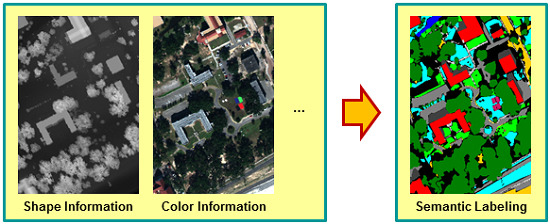
Geospatial Computer Vision Based on Multi-Modal Data—How Valuable Is Shape Information for the Extraction of Semantic Information?

1
Institute of Photogrammetry and Remote Sensing, Karlsruhe Institute of Technology (KIT), Englerstr. 7, D-76131 Karlsruhe, Germany
2
Institute of Computer Science II, University of Bonn, Friedrich-Ebert-Allee 144, D-53113 Bonn, Germany
*
Author to whom correspondence should be addressed.
Remote Sens. 2018, 10(1), 2; https://doi.org/10.3390/rs10010002
Submission received: 12 October 2017
/
Revised: 11 December 2017
/
Accepted: 17 December 2017
/
Published: 21 December 2017
(This article belongs to the Special Issue 3D Reconstruction & Semantic Information from Aerial and Satellite Images)
Abstract
:In this paper, we investigate the value of different modalities and their combination for the analysis of geospatial data of low spatial resolution. For this purpose, we present a framework that allows for the enrichment of geospatial data with additional semantics based on given color information, hyperspectral information, and shape information. While the different types of information are used to define a variety of features, classification based on these features is performed using a random forest classifier. To draw conclusions about the relevance of different modalities and their combination for scene analysis, we present and discuss results which have been achieved with our framework on the MUUFL Gulfport Hyperspectral and LiDAR Airborne Data Set.
1. Introduction
Geospatial computer vision deals with the acquisition, exploration, and analysis of our natural and/or man-made environments. This is of great importance for many applications such as land cover and land use classification, semantic reconstruction, or abstractions of scenes for city modeling. While different scenes may generally exhibit different levels of complexity, there are also various different sensor types that allow for the capture of significantly different scene characteristics. As a result, the captured data may be represented in various forms such as imagery or point clouds, and acquired spatial (i.e., geometric), spectral, and radiometric data might be given at different resolutions. The use of these individual types of geospatial data as well as different combinations is of particular interest for the acquisition and analysis of urban scenes which provide a rich diversity of both natural and man-made objects.
A ground-based acquisition of urban scenes nowadays typically relies on the use of mobile laser scanning (MLS) systems [1,2,3,4] or terrestrial laser scanning (TLS) systems [5,6]. While this delivers a dense sampling of object surfaces, achieving a full coverage of the considered scene is challenging, as the acquisition system has to be moved through the scene either continuously (in the case of an MLS system) or with relatively small displacements of a few meters (in the case of a TLS system) to handle otherwise occluded parts of the scene. Consequently, the considered area tends to be rather small, i.e., only street sections or districts are covered. Furthermore, the dense sampling often results in a massive amount of geospatial data that has to be processed. In contrast, the use of airborne platforms equipped with airborne laser scanning (ALS) systems allows for the acquisition of geospatial data corresponding to large areas of many km. However, the sampling of object surfaces is not that dense, with only a few tens of measured points per m. The lower point density in turn makes semantic scene interpretation more challenging as the local geometric structure may be quite similar for different classes. To address this lack with respect to the spatial resolution, additional devices such as cameras or spectrometers are often involved to capture standard color imagery or hyperspectral imagery in addition to 3D point cloud data. In this regard, however, there is still a lack regarding the relevance assessment of the different modalities and their combination for scene analysis.
1.1. Contribution
In this paper, we investigate the value of different modalities of geospatial data acquired from airborne platforms for scene analysis in terms of a semantic labeling with respect to user-defined classes. For this purpose, we use a benchmark dataset for which different types of information are available: color information, hyperspectral information, and shape information. Using these types of information separately and in different combinations, we define feature vectors and classify them with a random forest classifier. This allows us to reason about the relevance of each modality as well as the relevance of multi-modal data for the semantic labeling task. Thereby, we focus in particular on analyzing how valuable shape information is for the extraction of semantic information in challenging scenarios of low point density. Furthermore, we take into account that, in practical applications, e.g., focusing on land cover and land use classification, we additionally face the challenge of a classification task where only very few training data are available to train a classifier. This is due to the fact that expert knowledge might be required for an appropriate labeling (particularly when using hyperspectral data) and the annotation process may hence be costly and time-consuming. To address such issues, we focus on the use of sparse training data of only few training examples per class. In summary, the key contributions of our work are:
- the robust extraction of semantic information from geospatial data of low spatial resolution;
- the investigation of the relevance of color information, hyperspectral information, and shape information for the extraction of semantic information;
- the investigation of the relevance of multi-modal data comprising hyperspectral information and shape information for the extraction of semantic information; and
- the consideration of a semantic labeling task given only very sparse training data.
A parallelized, but not fully optimized Matlab implementation for the extraction of all presented geometric features is available at http://www.ipf.kit.edu/code.php.
After briefly summarizing related work in Section 1.2, we present our framework for scene analysis based on multi-modal data in Section 2. Subsequently, in Section 3, we demonstrate the performance of our framework by evaluation on a benchmark dataset with a specific focus on how valuable shape information is for the considered classification task. This is followed by a discussion of the derived results in Section 4. Finally, we provide concluding remarks in Section 5.
1.2. Related Work
In recent years, the acquisition and analysis of geospatial data has been addressed by numerous investigations. Among a range of addressed research topics, particular attention has been paid to the semantic interpretation of 3D data acquired via MLS, TLS, or ALS systems within urban areas [1,2,3,4,6,7,8,9,10,11] which is an important prerequisite for a variety of high-level tasks such as city modeling and planning. In such a scenario, the acquired 3D data corresponds to a dense sampling of object surfaces preserving many details of the geometric structure. Thus, the main challenges for scene analysis are typically represented by the irregular point sampling and the complexity of the observed scene. Numerous investigations on interpreting such data focused on a data-driven extraction of local neighborhoods as the basis for feature extraction (Section 1.2.1), on the extraction of suitable features (Section 1.2.2), and on the classification process itself (Section 1.2.3).
1.2.1. Neighborhood Selection
When using geometric features for scene analysis, it has to be taken into account that such features are used to describe the local 3D structure and hence are extracted from the local arrangement of 3D points within a local neighborhood. For the latter, either a spherical neighborhood [12,13] or a cylindrical neighborhood [14] is typically selected. Such neighborhoods, in turn, can be parameterized with a single parameter. Assuming that a cylindrical neighborhood is aligned along the vertical direction, it is normally defined by two parameters: radius and height. When analyzing ALS data, however, the height is typically set as infinitely large. The remaining parameter is commonly referred to as the “scale” and in most cases represented by either a radius [12,14] or the number of nearest neighbors that are considered [13]. As a suitable value for the scale parameter may be different for different classes [7], it seems appropriate to involve a data-driven approach to select locally-adaptive neighborhoods of optimal size. Respective approaches for instance rely on the local surface variation [15] or the joint consideration of curvature, point density, and noise of normal estimation [16,17]. Further approaches are represented by dimensionality-based scale selection [18], and eigenentropy-based scale selection [7]. Both of these approaches focus on the minimization of a functional, which is defined in analogy to the Shannon entropy across different values of the scale parameter, and select the neighborhood size that delivers the minimum Shannon entropy.
Instead of selecting a single neighborhood as the basis for extracting geometric features [1,7,19], multi-scale neighborhoods may be involved to describe the local 3D geometry at different scales and thus also how the local 3D geometry changes across scales. In this regard, one may use multiple spherical neighborhoods [20], multiple cylindrical neighborhoods [10,21], or a multi-scale voxel representation [5]. Furthermore, multiple neighborhoods could be defined on the basis of different entities, e.g., in the form of both spherical and cylindrical neighborhoods [11], in the form of voxels, blocks, and pillars [22], or in the form of spatial bins, planar segments, and local neighborhoods [23].
In our work, we focus on the use of co-registered shape, color, and hyperspectral information corresponding to a discrete raster. This allows for data representations in the form of a height map, color imagery, and hyperspectral imagery. Consequently, we involve local image neighborhoods as the basis for extracting 2.5D shape information. For comparison, we also assess the local 3D neighborhood of optimal size for each 3D point individually as the basis for extracting 3D shape information. The use of multiple neighborhoods is not considered in the scope of our preliminary work on geospatial computer vision based on multi-modal data, but it should definitively be the subject of future work.
1.2.2. Feature Extraction
Among a variety of handcrafted geometric features that have been presented in different investigations, the local 3D shape features, which are represented by linearity, planarity, sphericity, omnivariance, anisotropy, eigenentropy, sum of eigenvalues, and local surface variation [15,24], are most widely used, since each of them describes a rather intuitive quantity with a single value. However, using only these features is often not sufficient to obtain appropriate classification results (in particular for more complex scenes) and therefore further characteristics of the local 3D structure are encoded with complementary features such as angular statistics [1], height and plane characteristics [9,25], low-level 3D and 2D features [7], or moments and height features [5].
Depending on the system used for data acquisition, complementary types of data may be recorded in addition to the geometric data. Respective data representations suited for scene analysis are for instance given by echo-based features [9,26], full-waveform features [9,26], or radiometric features [10,21,27]. The latter can be extracted by evaluating the backscattered reflectance at the wavelength with which the involved LiDAR sensor emits laser light. However, particularly for a more detailed scene analysis as for instance given by a fine-grained land cover and land use classification, multi- or hyperspectral data offer great potential. In this regard, hyperspectral information in particular has been in the focus of recent research on environmental mapping [28,29,30]. Such information can, for example, allow for distinguishing very different types of vegetation and to a certain degree also different materials, which can be helpful if the corresponding shape is similar. The use of data acquired with complementary types of sensors has for instance been proposed for building detection in terms of fusing ALS data and multi-spectral imagery [31]. Despite the fusion of data acquired with complementary types of sensors, technological advancements meanwhile allow the use of multi- or hyperspectral LiDAR sensors [27]. Based on the concept of multi-wavelength airborne laser scanning [32], two different LiDAR sensors have been used to collect dual-wavelength LiDAR data for land cover classification [33]. Here, the involved sensors emit pulses of light in the near-infrared domain and in the middle-infrared domain. Further investigations on land cover and land use classification involved a multi-wavelength airborne LiDAR system delivering 3D data as well as three reflectance images corresponding to the green, near-infrared, and short-wave infrared bands, using either three independent sensors [34], or a single sensor such as the Optech Titan sensor which carries three lasers of different wavelengths [34,35]. While the classification may also be based on spectral patterns [36] or different spectral indices [37,38], further work focused on the extraction of geometric and intensity features on the basis of segments for land cover classification and change detection [39,40,41]. Further improvements regarding scene analysis may be achieved via the use of multi-modal data in the form of co-registered hyperspectral imagery and 3D point cloud data for scene analysis. Such a combination has already proven to be beneficial for tree species classification [42] as well as for civil engineering and urban planning applications [43]. Furthermore, the consideration of multiple modalities allows for simultaneously addressing different tasks. In this regard, it has for instance been proposed to exploit color imagery, multispectral imagery, and thermal imagery acquired from an airborne platform for the mapping of moss beds in Antarctica [44]. On the one hand, the high-resolution color imagery allows an appropriate 3D reconstruction of the considered scene in the form of a high-resolution digital terrain model and the creation of a photo-realistic 3D model. On the other hand, the multispectral imagery and thermal imagery allow for drawing conclusions about the location and extent of healthy moss as well as about areas of potentially high water concentration.
Instead of relying on a set of handcrafted features, recent approaches for point cloud classification focus on the use of deep learning techniques with which a semantic labeling is achieved via learned features. This may for instance be achieved via the transfer of the considered point cloud to a regular 3D voxel grid and the direct adaptation of convolutional neural networks (CNNs) to 3D data. In this regard, the most promising approaches rely on classifying each 3D point of a point cloud based on a transformation of all points within its local neighborhood to a voxel-occupancy grid serving as input for a 3D-CNN [6,45,46,47]. Alternatively, 2D image projections may be used as input for a 2D-CNN designed for semantic segmentation and a subsequent back-projection of predicted labels to 3D space delivers the semantically labeled 3D point cloud [48,49].
In our work, we focus on the separate and combined consideration of shape, color, and hyperspectral information. We extract a set of commonly used geometric features in 3D on the basis of a discrete image raster, and we extract spectral features in terms of Red-Green-Blue (RGB) color values, color invariants, raw hyperspectral signatures, and an encoding of hyperspectral information via the standard principal component analysis (PCA). Due to the limited amount of training data in the available benchmark data, only handcrafted features are considered, while the use of learned features will be subject of future work given larger benchmark datasets.
1.2.3. Classification
To classify the derived feature vectors, the straightforward approach consists in the use of standard supervised classification techniques such as support vector machines or random forest classifiers [5,7] which are meanwhile available in a variety of software tools and can easily be applied by non-expert users. Due to the individual consideration of feature vectors, however, the derived labeling reveals a “noisy” behavior when visualized as a colored point cloud, while a higher spatial regularity would be desirable since the labels of neighboring 3D points tend to be correlated.
To impose spatial regularity on the labeling, it has for instance been proposed to use associative and non-associative Markov networks [1,50,51], conditional random fields (CRFs) [10,52,53], multi-stage inference procedures relying on point cloud statistics and relational information across different scales [19], spatial inference machines modeling mid- and long-range dependencies inherent in the data [54], 3D entangled forests [55] or structured regularization representing a more versatile alternative to the standard graphical model approach [8]. Some of these approaches focus on directly classifying the 3D points, while others focus on a consideration of point cloud segments. In this regard, however, it has to be taken into account that the performance of segment-based approaches strongly depends on the quality of the achieved segmentation results and that a generic, data-driven 3D segmentation typically reveals a high computational burden. Furthermore, classification approaches enforcing spatial regularity generally require additional effort for inferring interactions among neighboring 3D points from the training data which, in most cases, corresponds to a larger amount of data that is needed to train a respective classifier.
Instead of a point-based classification and subsequent efforts for imposing spatial regularity on the labeling, some approaches also focus on the interplay between classification and segmentation. In this regard, many approaches start with an over-segmentation of the scene, e.g., by deriving supervoxels [56,57]. Based on the segments, features are extracted and then used as input for classification. In contrast, an initial point-wise classification may serve as input for a subsequent segmentation in order to detect specific objects in the scene [4,58,59] or to improve the labeling [60]. The latter has also been addressed with a two-layer CRF [52,61]. Here, the results of a CRF-based classification on point-level are used as input for a region-growing algorithm connecting points which are close to each other and meet additional conditions such as having the same label from the point-based classification. Subsequently, a further CRF-based classification is carried out on the basis of segments corresponding to connected points. While the two CRF-based classifications may be performed successively [61], it may be taken into account that the CRF-based classification on the segment level delivers a belief for each segment to belong to a certain class [52]. The beliefs in turn may be used to improve the CRF-based classification on the point level. Hence, performing the classification in both layers several times in an iterative scheme allows improving the segments and transferring regional context to the point-based level [52]. A different strategy has been followed by integrating a non-parametric segmentation model (which partitions the scene into geometrically-homogeneous segments) into a CRF in order to capture the high-level structure of the scene [62]. This allows aggregating the noisy predictions of a classifier on a per-segment basis in order to produce a data term of higher confidence.
In our work, we conduct experiments on a benchmark dataset allowing the separate and combined consideration of shape, color, and hyperspectral information. As only a limited amount of training data is given in the available data, we focus on point-based classification via a standard classifier, while the use of more sophisticated classification/regularization techniques will be subject of future work given larger benchmark datasets.
2. Materials and Methods
In this section, we present our framework for scene analysis based on multi-modal data in detail. The input for our framework is represented by co-registered multi-modal data containing color information, hyperspectral information, and shape information. The desired output is a semantic labeling with respect to user-defined classes. To achieve such a labeling, our framework involves feature extraction (Section 2.1) and supervised classification (Section 2.2).
2.1. Feature Extraction
Using the given color, hyperspectral and shape information, we extract the following features:
- Color information: We take into account that semantic image classification or segmentation often involves color information corresponding to the red (R), green (G), and blue (B) channels in the visible spectrum. Consequently, we define the feature set addressing the spectral reflectance I with respect to the corresponding spectral bands:Since RGB color representations are less robust with respect to changes in illumination, we additionally involve normalized colors also known as chromaticity values as a simple example of color invariants [63]:Furthermore, we use a color model which is invariant to viewing direction, object geometry, and shading under the assumptions of white illumination and dichromatic reflectance [63]:Among the more complex transformations of the RGB color space, we test the approaches represented by comprehensive color image normalization (CCIN) [64] resulting in and edge-based color constancy (EBCC) [65] resulting in .
- Hyperspectral information: We also consider spectral information at a multitude of spectral bands which typically cover an interval reaching from the visible spectrum to the infrared spectrum. Assuming hyperspectral image (HSI) data across n spectral bands with , we define the feature set addressing the spectral reflectance I of a pixel for all spectral bands:
- PCA-based encoding of hyperspectral information: Due to the fact that adjacent spectral bands typically reveal a high degree of redundancy, we transform the given hyperspectral data to a new space spanned by linearly uncorrelated meta-features using the standard principal component analysis (PCA). Thus, the most relevant information is preserved in those meta-features indicating the highest variability of the given data. For our work, we sort the meta-features with respect to the covered variability and then use the set of the m most relevant meta-features with which covers % of the variability of the given data:
- 3D shape information: From the coordinates acquired via airborne laser scanning and transformed to a regular grid, we extract a set of intuitive geometric features for each 3D point whose behavior can easily be interpreted by the user [7]. As such features describe the spatial arrangement of points in a local neighborhood, a suitable neighborhood has to be selected first for each 3D point. To achieve this, we apply eigenentropy-based scale selection [7] which has proven to be favorable compared to other options for the task of point cloud classification. For each 3D point , this algorithm derives the optimal number of nearest neighbors with respect to the Euclidean distance in 3D space. Thereby, for each case specified by the tested value of the scale parameter , the algorithm uses the spatial coordinates of and its neighboring points to compute the 3D structure tensor and its eigenvalues. The eigenvalues are then normalized by their sum, and the normalized eigenvalues with are used to calculate the eigenentropy (i.e., the disorder of 3D points within a local neighborhood). The optimal scale parameter is finally derived by selecting the scale parameter that corresponds to the minimum eigenentropy across all cases:Thereby, contains all integer values in with as lower boundary for allowing meaningful statistics and as upper boundary for limiting the computational effort [7].Based on the derived local neighborhood of each 3D point , we extract a set comprising 18 rather intuitive features which are represented by a single value per feature [7]. Some of these features rely on the normalized eigenvalues of the 3D structure tensor and are represented by linearity , planarity , sphericity , omnivariance , anisotropy , eigenentropy , sum of eigenvalues , and local surface variation [15,24]. Furthermore, the coordinate , indicating the height of , is used as well as the distance between and the farthest point in the local neighborhood. Additional features are represented by the local point density , the verticality , and the maximum difference and standard deviation of the height values of those points within the local neighborhood. To account for the fact that urban areas in particular are characterized by an aggregation of many man-made objects with many (almost) vertical surfaces, we encode specific properties by projecting the 3D point and its nearest neighbors onto a horizontal plane. From the 2D projections, we derive the 2D structure tensor and its eigenvalues. Then, we define the sum and the ratio of these eigenvalues as features. Finally, we use the 2D projections of and its nearest neighbors to derive the distance between the projection of and the farthest point in the local 2D neighborhood, and the local point density in 2D space. For more details on these features, we refer to [7]. Using all these features, we define the feature set :
- 2.5D shape information: Instead of the pure consideration of 3D point distributions and corresponding 2D projections, we also directly exploit the grid structure of the provided imagery to define local image neighborhoods. Based on the corresponding coordinates, we derive the features of linearity , planarity , sphericity , omnivariance , anisotropy , eigenentropy , sum of eigenvalues , and local surface variation in analogy to the 3D case. Similarly, we define the maximum difference and standard deviation of the height values of those points within the local image neighborhood as features:
- Multi-modal information: Instead of separately considering the different modalities, we also consider a meaningful combination, i.e., multi-modal data, with the expectation that the complementary types of information significantly alleviate the classification task. Regarding spectral information, the PCA-based encoding of hyperspectral information is favorable, because redundancy is removed and RGB information is already considered. Regarding shape information, both 3D and 2.5D shape information can be used. Consequently, we use the features derived via PCA-based encoding of hyperspectral information, the features providing 3D shape information, and the features providing 2.5D shape information as feature set :For comparison only, we use the feature set as a straightforward combination of color and 3D shape information, and the feature set as a straightforward combination of hyperspectral and 3D shape information:Furthermore, we involve the combination of color/hyperspectral information and 2.5D shape information as well as the combination of 3D and 2.5D shape information in our experiments:
In total, we test 15 different feature sets for scene analysis. For each feature set, the corresponding features are concatenated to derive a feature vector per data point.
2.2. Classification
To classify the derived feature vectors, we use a random forest (RF) classifier [66] as a representative of modern discriminative methods [67]. The RF classifier is trained by selecting random subsets of the training data and training a decision tree for each of the subsets. For a new feature vector, each decision tree casts a vote for one of the defined classes so that the majority vote across all decision trees represents a robust assignment.
For our experiments, we use an open-source implementation of the RF classifier [68]. To derive appropriate settings of the classifier (which address the number of involved decision trees, the maximum tree depth, the minimum number of samples to allow a node to be split, etc.), we use the training data and conduct an optimization via grid search on a suitable subspace.
3. Results
In the following, we present the involved dataset (Section 3.1), the used evaluation metrics (Section 3.2), and the derived results (Section 3.3).
3.1. Dataset
We evaluate the performance of our framework using the MUUFL Gulfport Hyperspectral and LiDAR Airborne Data Set [69] and a corresponding labeling of the scene [70] shown in Figure 1. The dataset comprises co-registered hyperspectral and LiDAR data which were acquired in November 2010 over the University of Southern Mississippi Gulf Park Campus in Long Beach, Mississippi, USA. According to the specifications, the hyperspectral data were acquired with an ITRES CASI-1500 and correspond to 72 spectral bands covering the wavelength interval between nm and nm with a varying spectral sampling ( nm to nm) [71]. Since the first four bands and the last four bands were characterized by noise, they were removed. The LiDAR data were acquired with an Optech Gemini ALTM relying on a laser with a wavelength of 1064 nm. The provided reference labeling addresses 11 semantic classes and a remaining class for unlabeled data. All data are provided on a discrete image grid of pixels, where a pixel corresponds to an area of 1 m × 1 m.
3.2. Evaluation Metrics
To evaluate the performance of different configurations of our framework, we compared the respectively derived labeling to the reference labeling on a per-point basis. Thereby, we consider the evaluation metrics represented by the overall accuracy , the kappa value , and the unweighted average of the -scores across all classes. To reason about the performance for single classes, we furthermore consider the classwise evaluation metrics represented by recall R and precision P.
3.3. Results
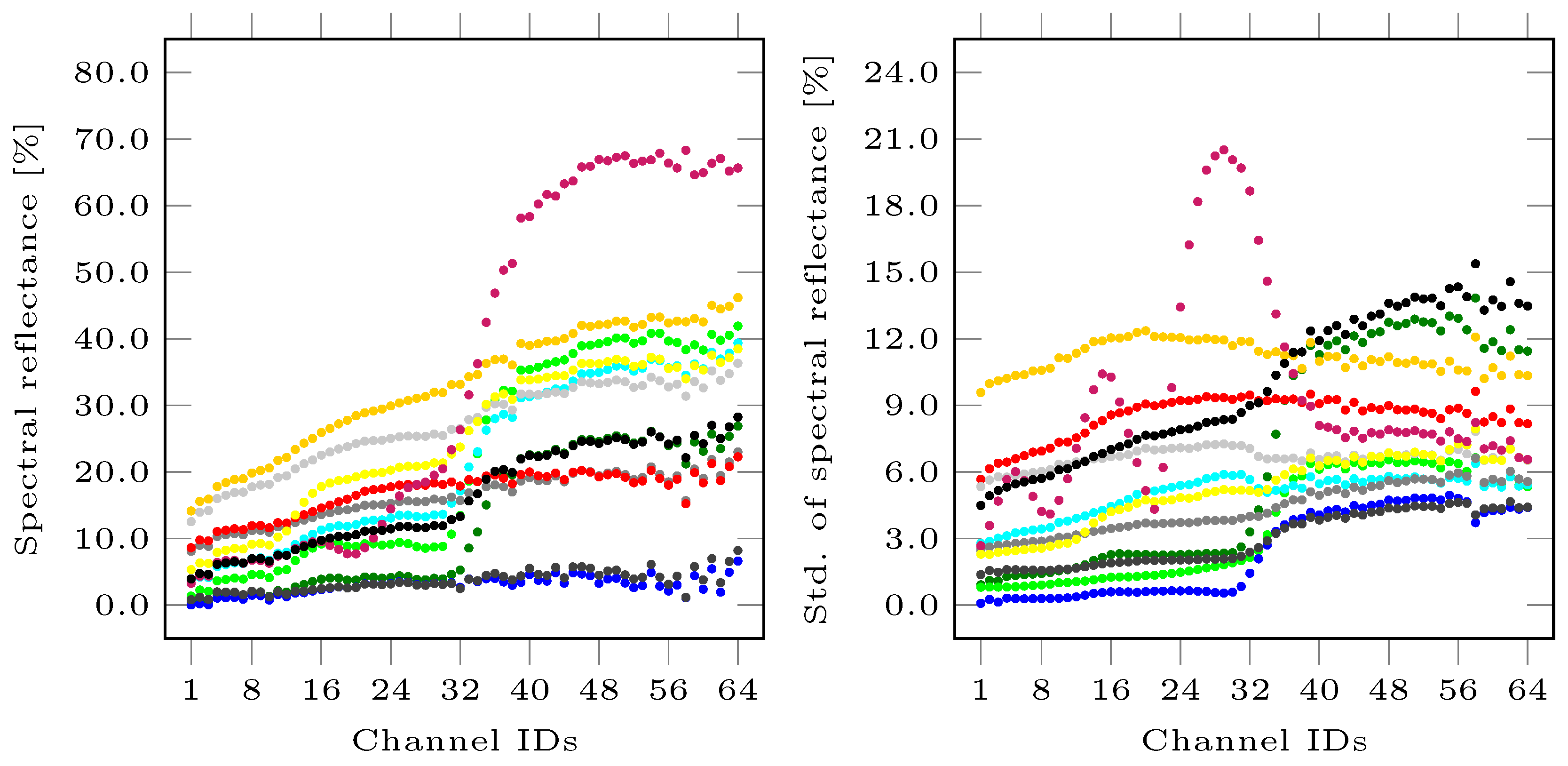
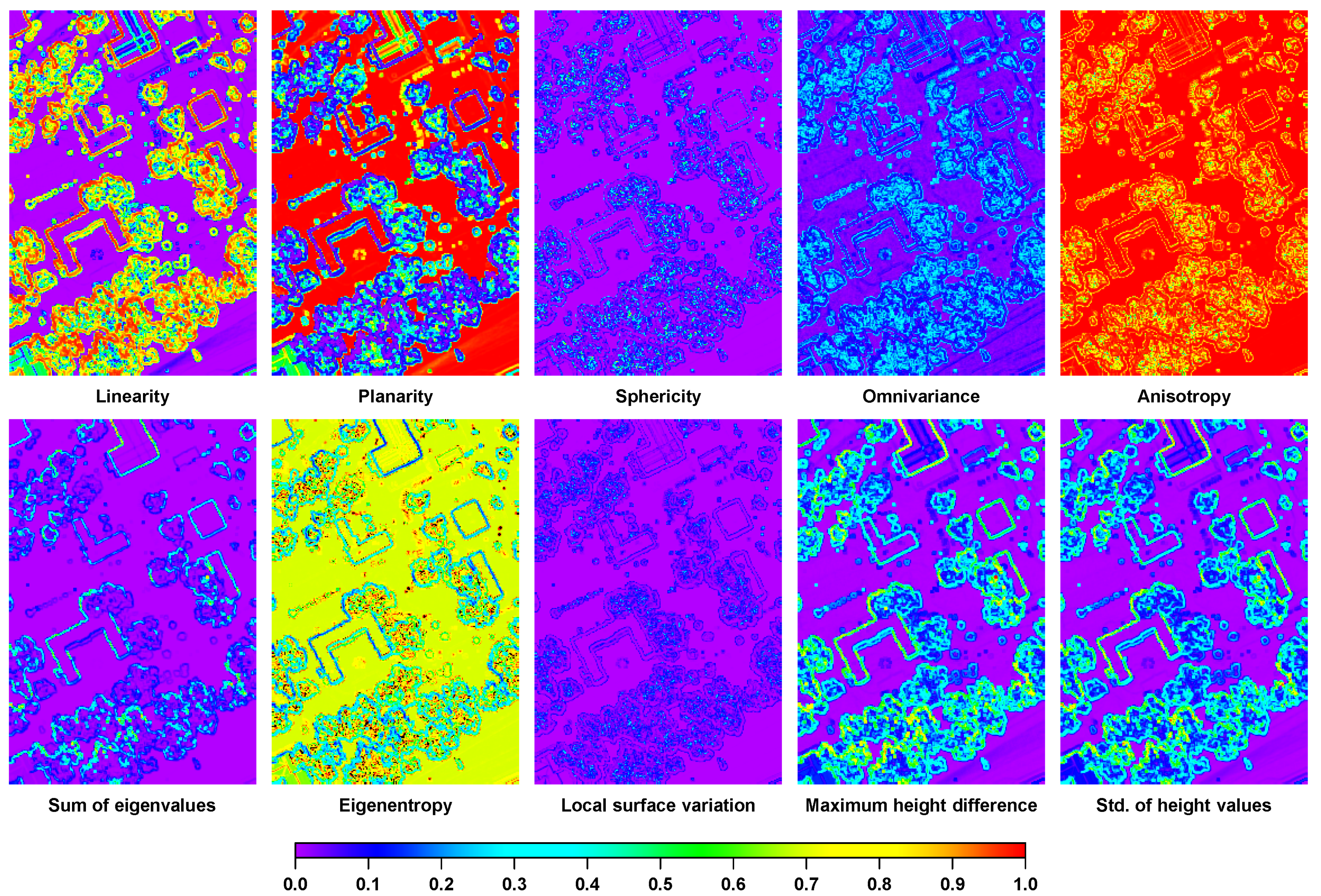
First, we focus on the behavior of derived features for different classes. Exploiting the hyperspectral signatures of all data points per class, we derive the mean spectra for the different classes as shown in the left part of Figure 2. The corresponding standard deviations per spectral band are shown in the right part of Figure 2 and reveal significant deviations for almost all classes. Regarding the shape information, a visualization of the derived 2.5D shape information is given in Figure 3, while a visualization of exemplary 3D features is given in Figure 4.
Regarding the color information, it can be noticed that each of the mentioned transformations of the RGB color space results in a new color model with three components. Accordingly, the result of each transformation can be visualized in the form of a color image as shown in Figure 5. Note that the applied transformations reveal quite different characteristics. The representation derived via edge-based color constancy (EBCC) [65] is visually quite similar to the original RGB color representation.
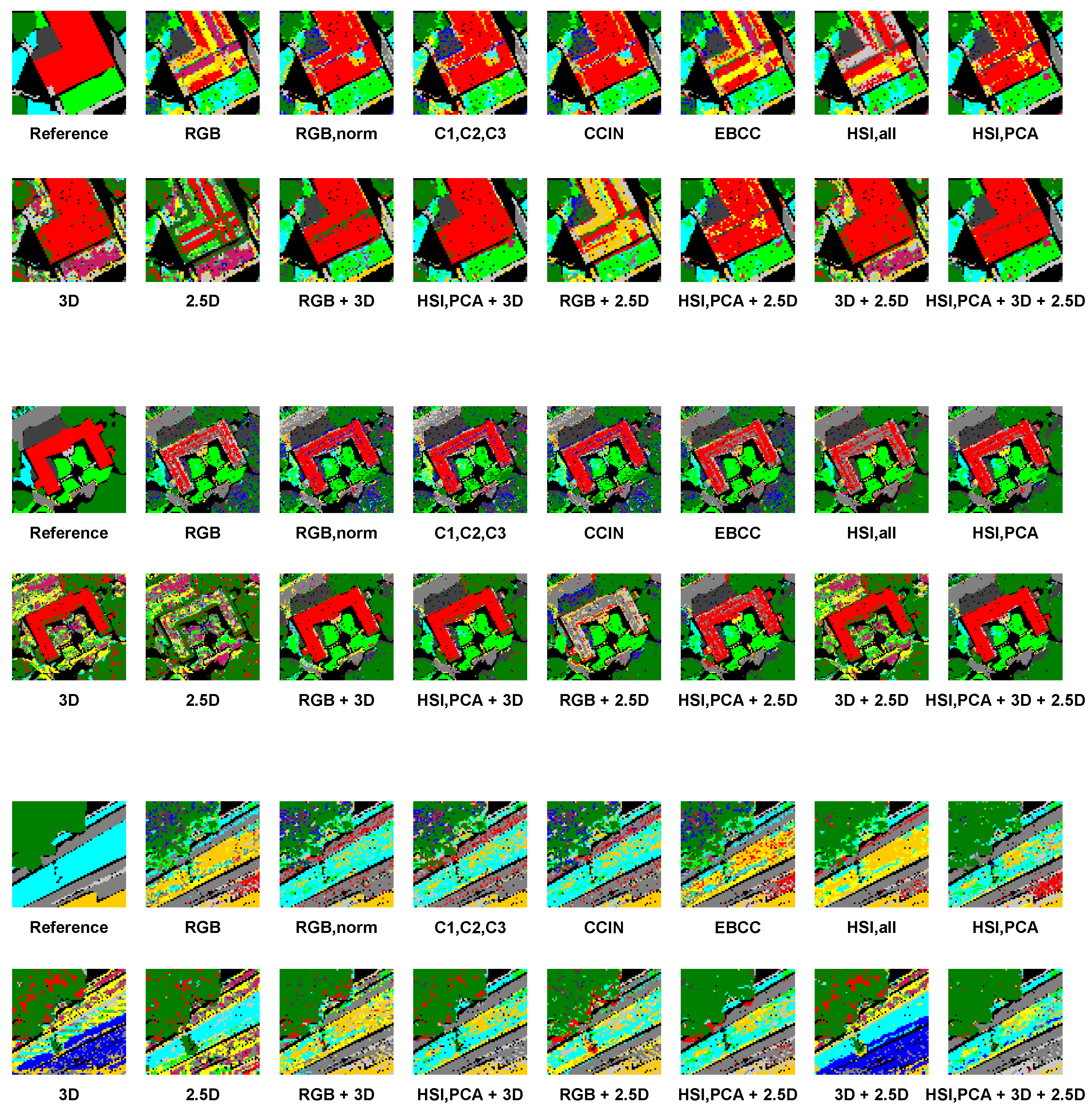
In the next step, we split the given dataset with data points into disjoint sets of training examples used for training the involved classifier and test examples used for performance evaluation. First of all, we discard data points that are labeled as C12 (“unlabeled”), because they might contain examples of different other classes (c.f. black curves in Figure 2) and hence not lead to an appropriate classification. Then, we randomly select 100 examples per remaining class to form balanced training data as suggested in [72] to avoid a negative impact of unbalanced data on the training process. The relatively small number of examples per class is realistic for practical applications focusing on scene analysis based on hyperspectral data [30]. All remaining examples are used as test data. To classify these test data, we define different configurations of our framework by selecting different feature sets as input for classification. For each configuration, the derived classification results are visualized in Figure 6. The corresponding values for the classwise evaluation metrics of recall R, precision P and -score are provided in Table 1, Table 2 and Table 3, respectively, and the values for the overall accuracy , the kappa value , and the unweighted average of the -scores across all classes are provided in Table 4.
4. Discussion
The derived results reveal that color and shape information alone are not sufficient to obtain appropriate classification results (c.f. Table 4). This is due to the fact that several classes are characterized by a similar color representation (c.f. Figure 1) or exhibit a similar geometric behavior when focusing on the local structure (c.f. Figure 3 and Figure 4). A closer look at the classwise evaluation metrics (c.f. Table 1, Table 2 and Table 3) reveals poor classification results for several classes, yet the transfer to different color representations (c.f. , , , and ) seems to be beneficial in comparison to the use of RGB color representations. In contrast, hyperspectral information allows for a better differentiation of the defined classes. However, it can be observed that a PCA should be applied to the hyperspectral data to remove redundancy which becomes visible in neighboring spectral bands that are highly correlated (c.f. Figure 2) and has a negative impact on classification (c.f. Table 4).
Furthermore, we can observe a clear benefit of the use of multi-modal data in comparison to the use of data of a single modality. The significant gain in , , and (c.f. Table 4) indicates both a better overall performance and a significantly better recognition of instances across all classes, which can indeed be verified by considering the classwise recall and precision values and -scores (c.f. Table 1, Table 2 and Table 3). The best performance is obtained when using the feature set representing a meaningful combination of hyperspectral information, 3D shape information, and 2.5D shape information.
In the following, we consider three exemplary parts of the scene in more detail. These parts are shown in Figure 7 and the corresponding classification results are visualized in Figure 8. The classification results derived for Area 1 are shown in the top part of Figure 8 and reveal that in particular the extracted 3D shape information can contribute to the detection of the given building, while the extracted 2.5D shape information is less suitable. For both cases, however, the different types of ground surfaces surrounding the building can hardly be correctly classified since other classes have a similar geometric behavior for the given grid resolution of 1 m. Using color and hyperspectral information, the surroundings of the building are better classified (particularly for the classes “mostly-grass ground surface” and “mixed ground surface”, but also for the classes “road” and “sidewalk”), while the correct classification of the building remains challenging with the RGB and EBCC representations. Even the use of all hyperspectral information is less suitable for this area, while the PCA-based encoding of hyperspectral information with lower dimensionality seems to be favorable. For Area 2, the derived classification results are shown in the center part of Figure 8. While the building can be correctly classified using 3D shape information, the use of 2.5D shape information hardly allows reasoning about the given building in this part of the scene. This might be due to the fact that the geometric properties in the respectively considered image neighborhoods are not sufficiently distinctive for the given grid resolution of 1 m. The data samples belonging to the flat roof of the building then appear similar to the data samples obtained for different types of flat ground surfaces. For the surrounding of the building, a similar behavior can be observed as for Area 1, since shape information remains less suitable to differentiate between different types of ground surfaces for the given grid resolution unless their roughness varies significantly. In contrast, color and hyperspectral information deliver a better classification of the observed area, but tend to partially interpret the flat roof as the “road”. This could be due to the fact that the material of the roof exhibits similar characteristics in the color and hyperspectral domains as the material of the road. For Area 3, the derived classification results are shown in the bottom part of Figure 8 and reveal that classes with a similar geometric behavior (e.g., the classes “mixed ground surface”, “dirt and sand”, “road” and “sidewalk”) can hardly be distinguished using only shape information. Some data samples are even classified as “water” which is also characterized by a flat surface, but is not present in this part of the scene. Using color information, the derived results seem to be better. With the RGB and EBCC representations, however, it still remains challenging to distinguish the classes “mixed ground surface” and “dirt and sand”, while the representation derived via simple normalization of the RGB components, the C1,C2,C3 representation, and the CCIN representation seem to perform much better in this regard. Involving hyperspectral information leads to a similar behavior as that visible for the use of color information for Area 3, but the classification results appear to be less “noisy”. For both color and hyperspectral information, some data samples are even classified as “roof”. This might be due to the fact that materials used for construction purposes exhibit similar characteristics in the color and hyperspectral domains as the materials of the given types of ground surfaces. Using data of different modalities for the classification of Areas 1–3, the derived classification results still reveal characteristics of the classification results derived with a separate consideration of the respective modalities. Yet, it becomes visible that the classification results have a less “noisy” behavior, and tend to be favorable in most cases. In summary, the extracted types of information reveal complementary characteristics. Shape information does not allow separating classes with a similar geometric behavior (e.g., the classes “mixed ground surface”, “dirt and sand”, “road” and “sidewalk”), yet particularly 3D shape information has turned out to provide a strong indication for buildings. In contrast, color information allows for the separation of classes with a different appearance, even if they exhibit a similar geometric behavior. This for instance allows separating natural ground surfaces (e.g., represented by the classes “mixed ground surface” and “dirt and sand”) from man-made ground surfaces (e.g., represented by the classes “road” and “sidewalk”). The used hyperspectral information covers the visible domain and the near-infrared domain for the given dataset. Accordingly, it should generally allow a better separation of different classes. This indeed becomes visible for the PCA-based encoding, but the use of all available hyperspectral information is not appropriate here due to the curse of dimensionality. Consequently, the combination of shape information and a PCA-based encoding of hyperspectral information is to be favored for the extraction of semantic information.
Regarding feature extraction, the RGB color information and the hyperspectral information across all spectral bands can directly be assessed from the given data. Processing times required to transform RGB color representations using the different color models are not significant. For the remaining options, we observed processing times of s for the PCA-based encoding of hyperspectral information, s for eigenentropy-based scale selection, s for extracting 3D shape information, and s for extracting 2.5D shape information on a standard laptop computer (Intel Core i7-6820HK, GHz, 4 cores, 16 GB RAM, Matlab implementation). In addition, s were required for training the RF classifier and s for classifying the test data.
We also want to point out that, in the scope of our experiments, we focused on rather intuitive geometric features that can easily be interpreted by the user. A straightforward extension would be the extraction of geometric features at multiple scales [5,10,20] and possibly different neighborhood types [11,22]. Furthermore, more complex geometric features could be considered [11] or deep learning techniques could be applied to learn appropriate features from 3D data [6]. Instead of addressing feature extraction, future efforts may also address the consideration of spatial regularization techniques [8,10,52,67] to address the fact that neighboring data points tend to be correlated and hence derive a smooth labeling. While all these issues are currently addressed in ongoing work, solutions for geospatial data with low spatial resolution and only few training examples still need to be addressed. Our work delivers important insights for further investigations in that regard.
5. Conclusions
In this paper, we have addressed scene analysis based on multi-modal data. Using color information, hyperspectral information, and shape information separately and in different combinations, we defined feature vectors and classified them with a random forest classifier. The derived results clearly reveal that shape information alone is of rather limited value for extracting semantic information if the spatial resolution is relatively low and if user-defined classes reveal a similar geometric behavior of the local structure. In such scenarios, the consideration of hyperspectral information in particular reveals a high potential for scene analysis, but still typically suffers from not considering the topography of the considered scene due to the use of a device operating in push-broom mode (e.g., like the visible and near-infrared (VNIR) push-broom sensor ITRES CASI-1500 involving a sensor array with 1500 pixels to scan a narrow across-track line on the ground). To address this issue, modern hyperspectral frame cameras could be used to directly acquire hyperspectral imagery and, if the geometric resolution is sufficiently high, 3D surfaces could even be reconstructed from the hyperspectral imagery, e.g., via stereophotogrammetric or structure-from-motion techniques [73]. Furthermore, the derived results indicate that, in contrast to the use of data of a single modality, the consideration of multi-modal data represented by hyperspectral information and shape information allows deriving appropriate classification results even for challenging scenarios with low spatial resolution.
Acknowledgments
We acknowledge support by Deutsche Forschungsgemeinschaft and Open Access Publishing Fund of Karlsruhe Institute of Technology.
Author Contributions
The authors jointly contributed to the concept of this paper, the implementation of the framework, the evaluation of the framework on a benchmark dataset, the discussion of derived results, and the writing of the paper.
Conflicts of Interest
The authors declare no conflict of interest.
References
- Munoz, D.; Bagnell, J.A.; Vandapel, N.; Hebert, M. Contextual classification with functional max-margin Markov networks. In Proceedings of the IEEE Conference on Computer Vision and Pattern Recognition, Miami, FL, USA, 20–25 June 2009; pp. 975–982. [Google Scholar]
- Serna, A.; Marcotegui, B.; Goulette, F.; Deschaud, J.E. Paris-rue-Madame database: A 3D mobile laser scanner dataset for benchmarking urban detection, segmentation and classification methods. In Proceedings of the International Conference on Pattern Recognition Applications and Methods, Angers, France, 6–8 March 2014; pp. 819–824. [Google Scholar]
- Brédif, M.; Vallet, B.; Serna, A.; Marcotegui, B.; Paparoditis, N. TerraMobilita/IQmulus urban point cloud classification benchmark. In Proceedings of the IQmulus Workshop on Processing Large Geospatial Data, Cardiff, UK, 8 July 2014; pp. 1–6. [Google Scholar]
- Gorte, B.; Oude Elberink, S.; Sirmacek, B.; Wang, J. IQPC 2015 Track: Tree separation and classification in mobile mapping LiDAR data. Int. Arch. Photogramm. Remote Sens. Spat. Inf. Sci. 2015, XL-3/W3, 607–612. [Google Scholar] [CrossRef]
- Hackel, T.; Wegner, J.D.; Schindler, K. Fast semantic segmentation of 3D point clouds with strongly varying density. ISPRS Ann. Photogramm. Remote Sens. Spat. Inf. Sci. 2016, III-3, 177–184. [Google Scholar] [CrossRef]
- Hackel, T.; Savinov, N.; Ladicky, L.; Wegner, J.D.; Schindler, K.; Pollefeys, M. Semantic3D.net: A new large-scale point cloud classification benchmark. ISPRS Ann. Photogramm. Remote Sens. Spat. Inf. Sci. 2017, IV-1/W1, 91–98. [Google Scholar] [CrossRef]
- Weinmann, M. Reconstruction and Analysis of 3D Scenes—From Irregularly Distributed 3D Points to Object Classes; Springer: Cham, Switzerland, 2016. [Google Scholar]
- Landrieu, L.; Raguet, H.; Vallet, B.; Mallet, C.; Weinmann, M. A structured regularization framework for spatially smoothing semantic labelings of 3D point clouds. ISPRS J. Photogramm. Remote Sens. 2017, 132, 102–118. [Google Scholar] [CrossRef]
- Mallet, C.; Bretar, F.; Roux, M.; Soergel, U.; Heipke, C. Relevance assessment of full-waveform LiDAR data for urban area classification. ISPRS J. Photogramm. Remote Sens. 2011, 66, S71–S84. [Google Scholar] [CrossRef]
- Niemeyer, J.; Rottensteiner, F.; Soergel, U. Contextual classification of LiDAR data and building object detection in urban areas. ISPRS J. Photogramm. Remote Sens. 2014, 87, 152–165. [Google Scholar] [CrossRef]
- Blomley, R.; Weinmann, M. Using multi-scale features for the 3D semantic labeling of airborne laser scanning data. ISPRS Ann. Photogramm. Remote Sens. Spat. Inf. Sci. 2017, IV-2/W4, 43–50. [Google Scholar] [CrossRef]
- Lee, I.; Schenk, T. Perceptual organization of 3D surface points. Int. Arch. Photogramm. Remote Sens. Spat. Inf. Sci. 2002, XXXIV-3A, 193–198. [Google Scholar]
- Linsen, L.; Prautzsch, H. Local versus global triangulations. In Proceedings of the Eurographics, Manchester, UK, 5–7 September 2001; pp. 257–263. [Google Scholar]
- Filin, S.; Pfeifer, N. Neighborhood systems for airborne laser data. Photogramm. Eng. Remote Sens. 2005, 71, 743–755. [Google Scholar] [CrossRef]
- Pauly, M.; Keiser, R.; Gross, M. Multi-scale feature extraction on point-sampled surfaces. Comput. Graph. Forum 2003, 22, 81–89. [Google Scholar] [CrossRef]
- Mitra, N.J.; Nguyen, A. Estimating surface normals in noisy point cloud data. In Proceedings of the Annual Symposium on Computational Geometry, San Diego, CA, USA, 8–10 June 2003; pp. 322–328. [Google Scholar]
- Lalonde, J.F.; Unnikrishnan, R.; Vandapel, N.; Hebert, M. Scale selection for classification of point-sampled 3D surfaces. In Proceedings of the International Conference on 3-D Digital Imaging and Modeling, Ottawa, ON, Canada, 13–16 June 2005; pp. 285–292. [Google Scholar]
- Demantké, J.; Mallet, C.; David, N.; Vallet, B. Dimensionality based scale selection in 3D LiDAR point clouds. Int. Arch. Photogramm. Remote Sens. Spat. Inf. Sci. 2011, XXXVIII-5/W12, 97–112. [Google Scholar]
- Xiong, X.; Munoz, D.; Bagnell, J.A.; Hebert, M. 3-D scene analysis via sequenced predictions over points and regions. In Proceedings of the IEEE International Conference on Robotics and Automation, Shanghai, China, 9–13 May 2011; pp. 2609–2616. [Google Scholar]
- Brodu, N.; Lague, D. 3D terrestrial LiDAR data classification of complex natural scenes using a multi-scale dimensionality criterion: Applications in geomorphology. ISPRS J. Photogramm. Remote Sens. 2012, 68, 121–134. [Google Scholar] [CrossRef] [Green Version]
- Schmidt, A.; Niemeyer, J.; Rottensteiner, F.; Soergel, U. Contextual classification of full waveform LiDAR data in the Wadden Sea. IEEE Geosci. Remote Sens. Lett. 2014, 11, 1614–1618. [Google Scholar] [CrossRef]
- Hu, H.; Munoz, D.; Bagnell, J.A.; Hebert, M. Efficient 3-D scene analysis from streaming data. In Proceedings of the IEEE International Conference on Robotics and Automation, Karlsruhe, Germany, 6–10 May 2013; pp. 2297–2304. [Google Scholar]
- Gevaert, C.M.; Persello, C.; Vosselman, G. Optimizing multiple kernel learning for the classification of UAV data. Remote Sens. 2016, 8, 1025. [Google Scholar] [CrossRef]
- West, K.F.; Webb, B.N.; Lersch, J.R.; Pothier, S.; Triscari, J.M.; Iverson, A.E. Context-driven automated target detection in 3-D data. Proc. SPIE 2004, 5426, 133–143. [Google Scholar]
- Guo, B.; Huang, X.; Zhang, F.; Sohn, G. Classification of airborne laser scanning data using JointBoost. ISPRS J. Photogramm. Remote Sens. 2015, 100, 71–83. [Google Scholar] [CrossRef]
- Chehata, N.; Guo, L.; Mallet, C. Airborne LiDAR feature selection for urban classification using random forests. Int. Arch. Photogramm. Remote Sens. Spat. Inf. Sci. 2009, XXXVIII-3/W8, 207–212. [Google Scholar]
- Yan, W.Y.; Shaker, A.; El-Ashmawy, N. Urban land cover classification using airborne LiDAR data: A review. Remote Sens. Environ. 2015, 158, 295–310. [Google Scholar] [CrossRef]
- Plaza, A.; Benediktsson, J.A.; Boardman, J.W.; Brazile, J.; Bruzzone, L.; Camps-Valls, G.; Chanussot, J.; Fauvel, M.; Gamba, P.; Gualtieri, A.; et al. Recent advances in techniques for hyperspectral image processing. Remote Sens. Environ. 2009, 113, S110–S122. [Google Scholar] [CrossRef]
- Camps-Valls, G.; Tuia, D.; Bruzzone, L.; Benediktsson, J. Advances in hyperspectral image classification: Earth monitoring with statistical learning methods. IEEE Signal Process. Mag. 2014, 31, 45–54. [Google Scholar] [CrossRef]
- Keller, S.; Braun, A.C.; Hinz, S.; Weinmann, M. Investigation of the impact of dimensionality reduction and feature selection on the classification of hyperspectral EnMAP data. In Proceedings of the 8th Workshop on Hyperspectral Image and Signal Processing: Evolution in Remote Sensing, Los Angeles, CA, USA, 21–24 August 2016; pp. 1–5. [Google Scholar]
- Rottensteiner, F.; Trinder, J.; Clode, S.; Kubik, K. Building detection by fusion of airborne laser scanner data and multi-spectral images: Performance evaluation and sensitivity analysis. ISPRS J. Photogramm. Remote Sens. 2007, 62, 135–149. [Google Scholar] [CrossRef]
- Pfennigbauer, M.; Ullrich, A. Multi-wavelength airborne laser scanning. In Proceedings of the International LiDAR Mapping Forum, New Orleans, LA, USA, 7–9 February 2011; pp. 1–10. [Google Scholar]
- Wang, C.K.; Tseng, Y.H.; Chu, H.J. Airborne dual-wavelength LiDAR data for classifying land cover. Remote Sens. 2014, 6, 700–715. [Google Scholar] [CrossRef]
- Hopkinson, C.; Chasmer, L.; Gynan, C.; Mahoney, C.; Sitar, M. Multisensor and multispectral LiDAR characterization and classification of a forest environment. Can. J. Remote Sens. 2016, 42, 501–520. [Google Scholar] [CrossRef]
- Bakuła, K.; Kupidura, P.; Jełowicki, Ł. Testing of land cover classification from multispectral airborne laser scanning data. Int. Arch. Photogramm. Remote Sens. Spat. Inf. Sci. 2016, XLI-B7, 161–169. [Google Scholar]
- Wichmann, V.; Bremer, M.; Lindenberger, J.; Rutzinger, M.; Georges, C.; Petrini-Monteferri, F. Evaluating the potential of multispectral airborne LiDAR for topographic mapping and land cover classification. ISPRS Ann. Photogramm. Remote Sens. Spat. Inf. Sci. 2015, II-3/W5, 113–119. [Google Scholar] [CrossRef]
- Morsy, S.; Shaker, A.; El-Rabbany, A.; LaRocque, P.E. Airborne multispectral LiDAR data for land-cover classification and land/water mapping using different spectral indexes. ISPRS Ann. Photogramm. Remote Sens. Spat. Inf. Sci. 2016, III-3, 217–224. [Google Scholar] [CrossRef]
- Zou, X.; Zhao, G.; Li, J.; Yang, Y.; Fang, Y. 3D land cover classification based on multispectral LiDAR point clouds. Int. Arch. Photogramm. Remote Sens. Spat. Inf. Sci. 2016, XLI-B1, 741–747. [Google Scholar] [CrossRef]
- Ahokas, E.; Hyyppä, J.; Yu, X.; Liang, X.; Matikainen, L.; Karila, K.; Litkey, P.; Kukko, A.; Jaakkola, A.; Kaartinen, H.; et al. Towards automatic single-sensor mapping by multispectral airborne laser scanning. Int. Arch. Photogramm. Remote Sens. Spat. Inf. Sci. 2016, XLI-B3, 155–162. [Google Scholar] [CrossRef]
- Matikainen, L.; Hyyppä, J.; Litkey, P. Multispectral airborne laser scanning for automated map updating. Int. Arch. Photogramm. Remote Sens. Spat. Inf. Sci. 2016, XLI-B3, 323–330. [Google Scholar] [CrossRef]
- Matikainen, L.; Karila, K.; Hyyppä, J.; Litkey, P.; Puttonen, E.; Ahokas, E. Object-based analysis of multispectral airborne laser scanner data for land cover classification and map updating. ISPRS J. Photogramm. Remote Sens. 2017, 128, 298–313. [Google Scholar] [CrossRef]
- Puttonen, E.; Suomalainen, J.; Hakala, T.; Räikkönen, E.; Kaartinen, H.; Kaasalainen, S.; Litkey, P. Tree species classification from fused active hyperspectral reflectance and LiDAR measurements. For. Ecol. Manag. 2010, 260, 1843–1852. [Google Scholar] [CrossRef]
- Brook, A.; Ben-Dor, E.; Richter, R. Fusion of hyperspectral images and LiDAR data for civil engineering structure monitoring. In Proceedings of the 2nd Workshop on Hyperspectral Image and Signal Processing: Evolution in Remote Sensing, Reykjavik, Iceland, 14–16 June 2010; pp. 1–5. [Google Scholar]
- Lucieer, A.; Robinson, S.; Turner, D.; Harwin, S.; Kelcey, J. Using a micro-UAV for ultra-high resolution multi-sensor observations of Antarctic moss beds. Int. Arch. Photogramm. Remote Sens. Spat. Inf. Sci. 2012, XXXIX-B1, 429–433. [Google Scholar] [CrossRef]
- Hackel, T.; Savinov, N.; Ladicky, L.; Wegner, J.D.; Schindler, K.; Pollefeys, M. Large-Scale Point Cloud Classification Benchmark, 2016. Available online: http://www.semantic3d.net (accessed on 17 November 2016).
- Savinov, N. Point Cloud Semantic Segmentation via Deep 3D Convolutional Neural Network, 2017. Available online: https://github.com/nsavinov/semantic3dnet (accessed on 31 July 2017).
- Huang, J.; You, S. Point cloud labeling using 3D convolutional neural network. In Proceedings of the International Conference on Pattern Recognition, Cancun, Mexico, 4–8 December 2016; pp. 2670–2675. [Google Scholar]
- Boulch, A.; Le Saux, B.; Audebert, N. Unstructured point cloud semantic labeling using deep segmentation networks. In Proceedings of the Eurographics Workshop on 3D Object Retrieval, Lyon, France, 23–34 April 2017; pp. 17–24. [Google Scholar]
- Lawin, F.J.; Danelljan, M.; Tosteberg, P.; Bhat, G.; Khan, F.S.; Felsberg, M. Deep projective 3D semantic segmentation. In Proceedings of the 17th International Conference on Computer Analysis of Images and Patterns, Ystad, Sweden, 22–24 August 2017; pp. 95–107. [Google Scholar]
- Shapovalov, R.; Velizhev, A.; Barinova, O. Non-associative markov networks for 3D point cloud classification. Int. Arch. Photogramm. Remote Sens. Spat. Inf. Sci. 2010, XXXVIII-3A, 103–108. [Google Scholar]
- Najafi, M.; Taghavi Namin, S.; Salzmann, M.; Petersson, L. Non-associative higher-order Markov networks for point cloud classification. In Proceedings of the European Conference on Computer Vision, Zurich, Switzerland, 6–12 September 2017; pp. 500–515. [Google Scholar]
- Niemeyer, J.; Rottensteiner, F.; Soergel, U.; Heipke, C. Hierarchical higher order CRF for the classification of airborne LiDAR point clouds in urban areas. Int. Arch. Photogramm. Remote Sens. Spat. Inf. Sci. 2016, XLI-B3, 655–662. [Google Scholar] [CrossRef]
- Landrieu, L.; Mallet, C.; Weinmann, M. Comparison of belief propagation and graph-cut approaches for contextual classification of 3D LiDAR point cloud data. In Proceedings of the IEEE International Geoscience and Remote Sensing Symposium, Fort Worth, TX, USA, 23–28 July 2017; pp. 1–4. [Google Scholar]
- Shapovalov, R.; Vetrov, D.; Kohli, P. Spatial inference machines. In Proceedings of the IEEE Conference on Computer Vision and Pattern Recognition, Portland, OR, USA, 23–28 June 2013; pp. 2985–2992. [Google Scholar]
- Wolf, D.; Prankl, J.; Vincze, M. Enhancing semantic segmentation for robotics: The power of 3-D entangled forests. IEEE Robot. Autom. Lett. 2016, 1, 49–56. [Google Scholar] [CrossRef]
- Kim, B.S.; Kohli, P.; Savarese, S. 3D scene understanding by voxel-CRF. In Proceedings of the IEEE International Conference on Computer Vision, Sydney, Australia, 1–8 December 2013; pp. 1425–1432. [Google Scholar]
- Wolf, D.; Prankl, J.; Vincze, M. Fast semantic segmentation of 3D point clouds using a dense CRF with learned parameters. In Proceedings of the IEEE International Conference on Robotics and Automation, Seattle, WA, USA, 26–30 May 2015; pp. 4867–4873. [Google Scholar]
- Monnier, F.; Vallet, B.; Soheilian, B. Trees detection from laser point clouds acquired in dense urban areas by a mobile mapping system. ISPRS Ann. Photogramm. Remote Sens. Spat. Inf. Sci. 2012, I-3, 245–250. [Google Scholar] [CrossRef]
- Weinmann, M.; Weinmann, M.; Mallet, C.; Brédif, M. A classification–segmentation framework for the detection of individual trees in dense MMS point cloud data acquired in urban areas. Remote Sens. 2017, 9, 277. [Google Scholar] [CrossRef]
- Weinmann, M.; Hinz, S.; Weinmann, M. A hybrid semantic point cloud classification–segmentation framework based on geometric features and semantic rules. PFG Photogramm. Remote Sens. Geoinf. 2017, 85, 183–194. [Google Scholar] [CrossRef]
- Niemeyer, J.; Rottensteiner, F.; Soergel, U.; Heipke, C. Contextual classification of point clouds using a two-stage CRF. Int. Arch. Photogramm. Remote Sens. Spat. Inf. Sci. 2015, XL-3/W2, 141–148. [Google Scholar] [CrossRef]
- Guignard, S.; Landrieu, L. Weakly supervised segmentation-aided classification of urban scenes from 3D LiDAR point clouds. Int. Arch. Photogramm. Remote Sens. Spat. Inf. Sci. 2017, XLII-1/W1, 151–157. [Google Scholar] [CrossRef]
- Gevers, T.; Smeulders, A.W.M. Color based object recognition. In Proceedings of the International Conference on Image Analysis and Processing, Florence, Italy, 17–19 September 1997; pp. 319–326. [Google Scholar]
- Finlayson, G.D.; Schiele, B.; Crowley, J.L. Comprehensive colour image normalization. In Proceedings of the European Conference on Computer Vision, Freiburg, Germany, 2–6 June 1998; pp. 475–490. [Google Scholar]
- Van de Weijer, J.; Gevers, T.; Gijsenij, A. Edge-based color constancy. IEEE Trans. Image Process. 2007, 16, 2207–2214. [Google Scholar] [CrossRef] [PubMed]
- Breiman, L. Random forests. Mach. Learn. 2001, 45, 5–32. [Google Scholar] [CrossRef]
- Schindler, K. An overview and comparison of smooth labeling methods for land-cover classification. IEEE Trans. Geosci. Remote Sens. 2012, 50, 4534–4545. [Google Scholar] [CrossRef]
- Dollár, P. Piotr’s Computer Vision Matlab Toolbox (PMT), Version 3.50. Available online: https://github.com/pdollar/toolbox (accessed on 17 November 2016).
- Gader, P.; Zare, A.; Close, R.; Aitken, J.; Tuell, G. MUUFL Gulfport Hyperspectral and LiDAR Airborne Data Set; Technical Report; REP-2013-570; University of Florida: Gainesville, FL, USA, 2013. [Google Scholar]
- Du, X.; Zare, A. Technical Report: Scene Label Ground Truth Map for MUUFL Gulfport Data Set; Technical Report; University of Florida: Gainesville, FL, USA, 2017. [Google Scholar]
- Zare, A.; Jiao, C.; Glenn, T. Multiple instance hyperspectral target characterization. arXiv, 2016; arXiv:1606.06354v2. [Google Scholar]
- Criminisi, A.; Shotton, J. Decision Forests for Computer Vision and Medical Image Analysis; Springer: London, UK, 2013. [Google Scholar]
- Bareth, G.; Aasen, H.; Bendig, J.; Gnyp, M.L.; Bolten, A.; Jung, A.; Michels, R.; Soukkamäki, J. Low-weight and UAV-based hyperspectral full-frame cameras for monitoring crops: Spectral comparison with portable spectroradiometer measurements. PFG Photogramm. Fernerkund. Geoinf. 2015, 2015, 69–79. [Google Scholar] [CrossRef]
Figure 1.
MUUFL Gulfport Hyperspectral and LiDAR Airborne Data Set: RGB image (left); height map (center) and provided reference labeling (right).
Figure 1.
MUUFL Gulfport Hyperspectral and LiDAR Airborne Data Set: RGB image (left); height map (center) and provided reference labeling (right).

Figure 2.
Mean spectra of the considered classes across all 64 spectral bands (left) and standard deviations of the spectral reflectance for the considered classes across all 64 spectral bands (right). The color encoding is in accordance with the color encoding defined in Figure 1.
Figure 2.
Mean spectra of the considered classes across all 64 spectral bands (left) and standard deviations of the spectral reflectance for the considered classes across all 64 spectral bands (right). The color encoding is in accordance with the color encoding defined in Figure 1.

Figure 3.
Visualization of the derived 2.5D shape information. The values for the maximum height difference and the standard deviation of height values are normalized to the interval .
Figure 3.
Visualization of the derived 2.5D shape information. The values for the maximum height difference and the standard deviation of height values are normalized to the interval .

Figure 4.
Visualization of the derived 3D shape information for the features of linearity , planarity , and sphericity .
Figure 4.
Visualization of the derived 3D shape information for the features of linearity , planarity , and sphericity .
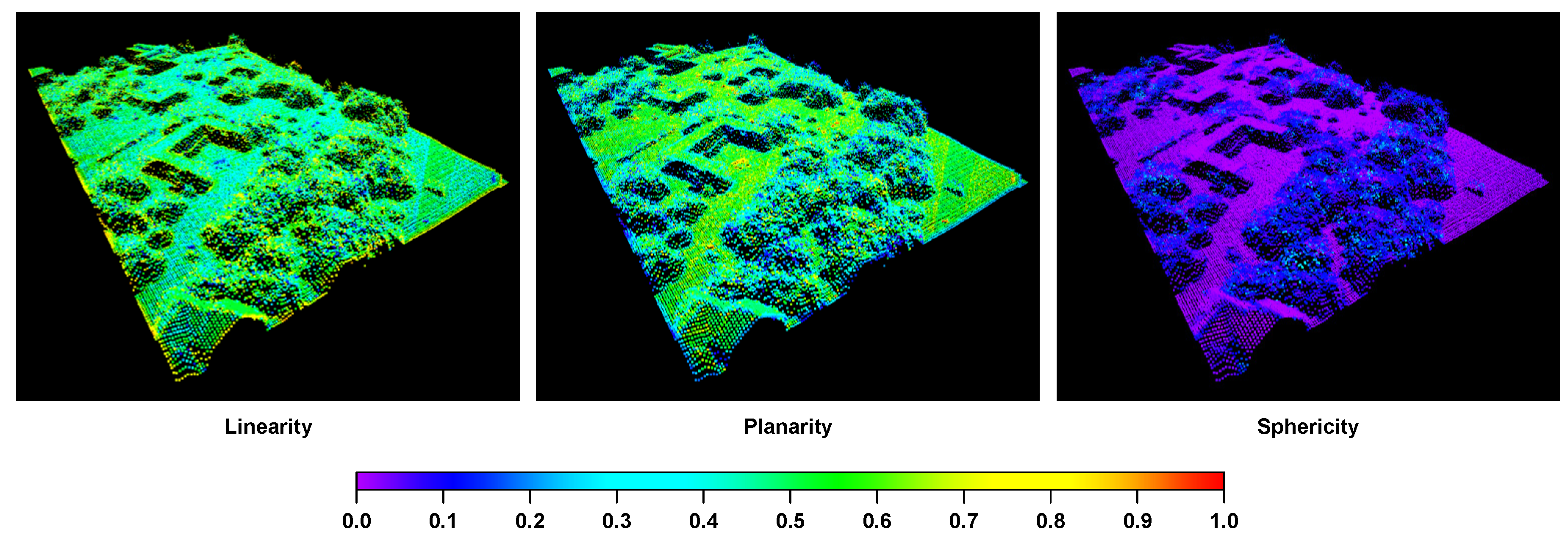
Figure 5.
Aerial image in different representations—the original image in the RGB color space and color-invariant representations derived via a simple normalization of the RGB components, the C1,C2,C3 color model proposed in [63], comprehensive color image normalization (CCIN) [64], and edge-based color constancy (EBCC) [65].

Figure 6.
Visualization of the reference labeling (top left) and the classification results derived for the MUUFL Gulfport Hyperspectral and LiDAR Airborne Data Set [69,70] by using the feature sets , , , , , , , , , , , , , , and (HSI: hyperspectral imagery; PCA: principal component analysis). The color encoding is in accordance with the color encoding defined in Figure 1.
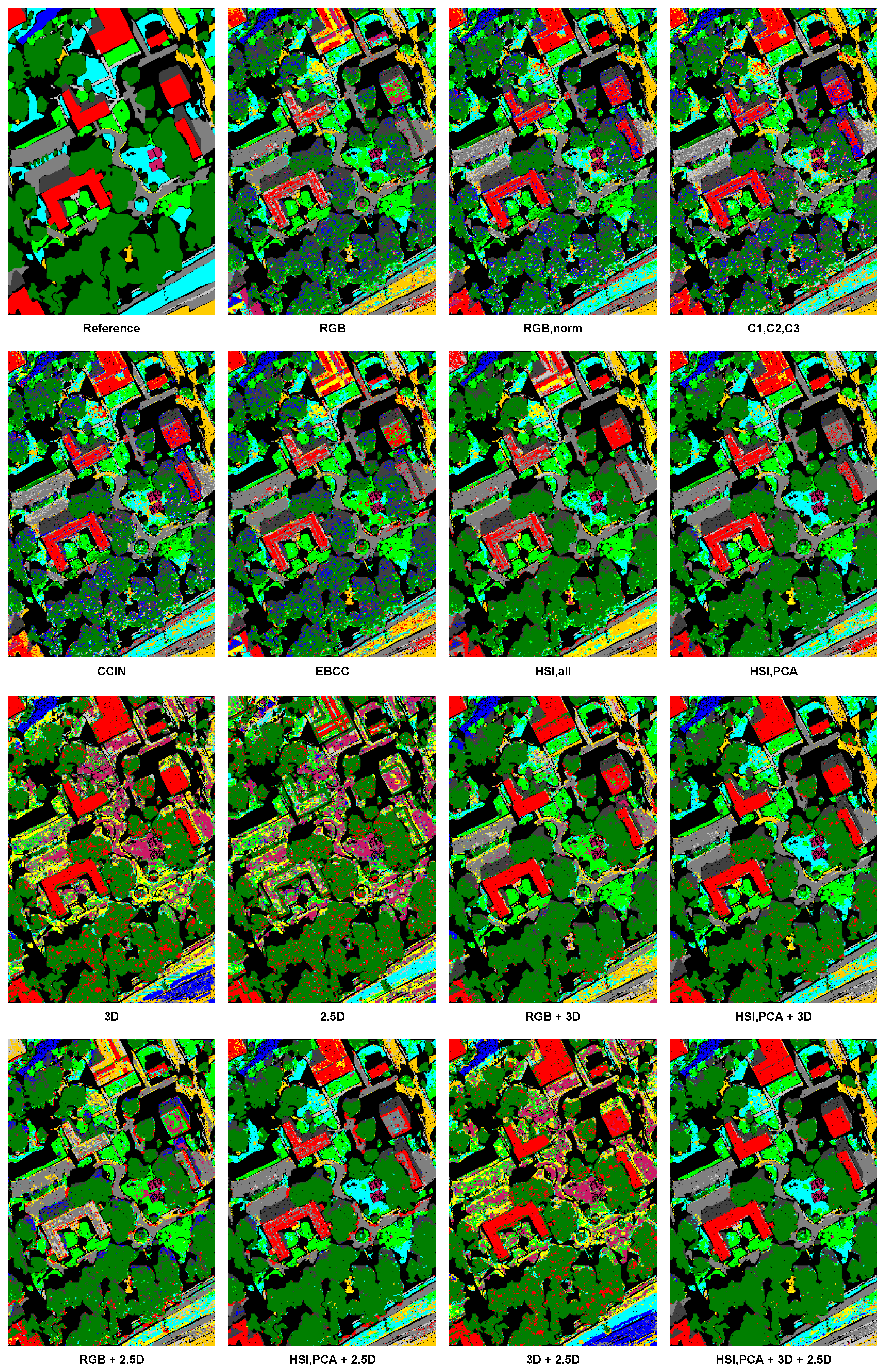
Figure 7.
Selection of three exemplary parts of the scene: Area 1 and Area 2 contain a building and its surrounding characterized by trees and different types of ground surfaces, while Area 3 contains a few trees and several types of ground surfaces.
Figure 7.
Selection of three exemplary parts of the scene: Area 1 and Area 2 contain a building and its surrounding characterized by trees and different types of ground surfaces, while Area 3 contains a few trees and several types of ground surfaces.
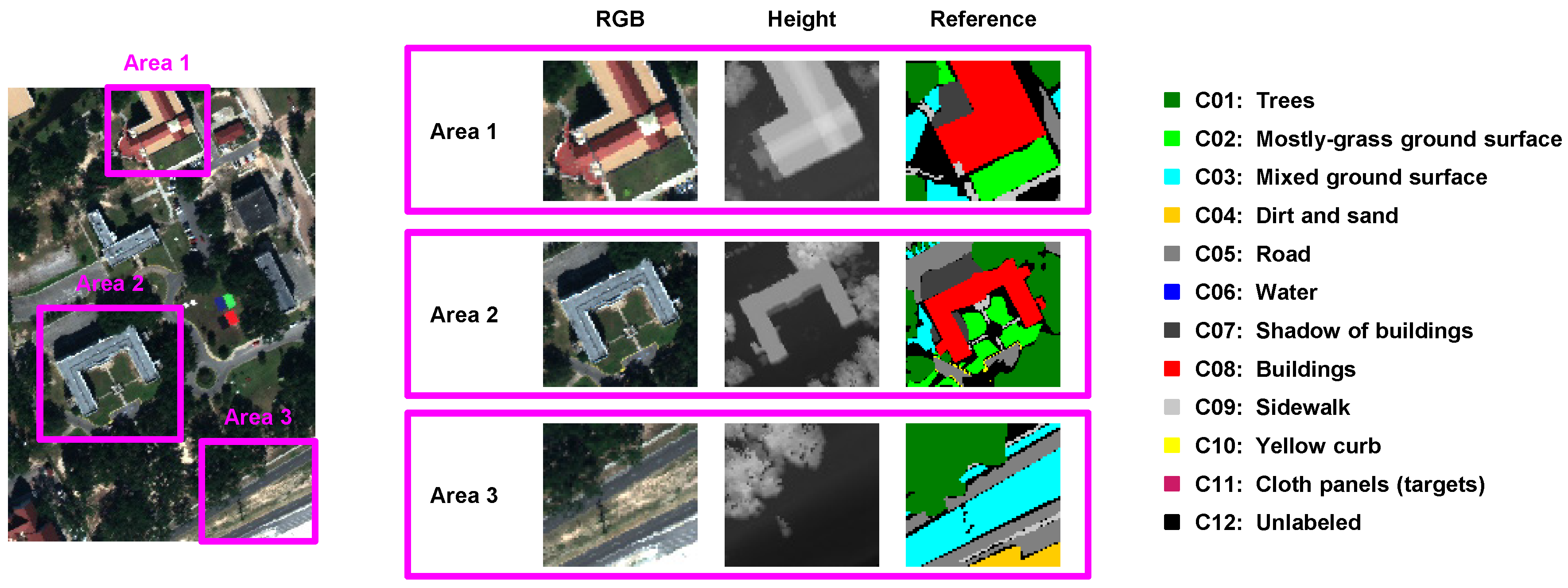
Figure 8.
Derived classification results for Area 1 (top); Area 2 (center) and Area 3 (bottom).


Table 1.
Recall values (in %) obtained for the semantic classes C01–C11 defined in Figure 1.
Table 1.
Recall values (in %) obtained for the semantic classes C01–C11 defined in Figure 1.
| Feature Set | C01 | C02 | C03 | C04 | C05 | C06 | C07 | C08 | C09 | C10 | C11 |
|---|---|---|---|---|---|---|---|---|---|---|---|
Table 2.
Precision values (in %) obtained for the semantic classes C01–C11 defined in Figure 1.
Table 2.
Precision values (in %) obtained for the semantic classes C01–C11 defined in Figure 1.
| Feature Set | C01 | C02 | C03 | C04 | C05 | C06 | C07 | C08 | C09 | C10 | C11 |
|---|---|---|---|---|---|---|---|---|---|---|---|
Table 3.
-scores (in %) obtained for the semantic classes C01–C11 defined in Figure 1.
Table 3.
-scores (in %) obtained for the semantic classes C01–C11 defined in Figure 1.
| Feature Set | C01 | C02 | C03 | C04 | C05 | C06 | C07 | C08 | C09 | C10 | C11 |
|---|---|---|---|---|---|---|---|---|---|---|---|
Table 4.
Classification results derived with different feature sets.
| Feature Set | OA [%] | [%] | [%] |
|---|---|---|---|
© 2017 by the authors. Licensee MDPI, Basel, Switzerland. This article is an open access article distributed under the terms and conditions of the Creative Commons Attribution (CC BY) license (http://creativecommons.org/licenses/by/4.0/).
Share and Cite
MDPI and ACS Style
Weinmann, M.; Weinmann, M. Geospatial Computer Vision Based on Multi-Modal Data—How Valuable Is Shape Information for the Extraction of Semantic Information? Remote Sens. 2018, 10, 2. https://doi.org/10.3390/rs10010002
AMA Style
Weinmann M, Weinmann M. Geospatial Computer Vision Based on Multi-Modal Data—How Valuable Is Shape Information for the Extraction of Semantic Information? Remote Sensing. 2018; 10(1):2. https://doi.org/10.3390/rs10010002
Chicago/Turabian StyleWeinmann, Martin, and Michael Weinmann. 2018. "Geospatial Computer Vision Based on Multi-Modal Data—How Valuable Is Shape Information for the Extraction of Semantic Information?" Remote Sensing 10, no. 1: 2. https://doi.org/10.3390/rs10010002
Note that from the first issue of 2016, this journal uses article numbers instead of page numbers. See further details here.