Assessing Different Feature Sets’ Effects on Land Cover Classification in Complex Surface-Mined Landscapes by ZiYuan-3 Satellite Imagery


1
Faculty of Computer Science and Geological Survey of CUG, China University of Geosciences, Wuhan 430074, China
2
Hubei Key Laboratory of Intelligent Geo-Information Processing, China University of Geosciences, Wuhan 430074, China
3
National Disaster Reduction Center of China, Beijing 100124, China
*
Authors to whom correspondence should be addressed.
Remote Sens. 2018, 10(1), 23; https://doi.org/10.3390/rs10010023
Submission received: 6 November 2017
/
Revised: 20 December 2017
/
Accepted: 22 December 2017
/
Published: 23 December 2017
(This article belongs to the Special Issue GIS and Remote Sensing advances in Land Change Science)
Abstract
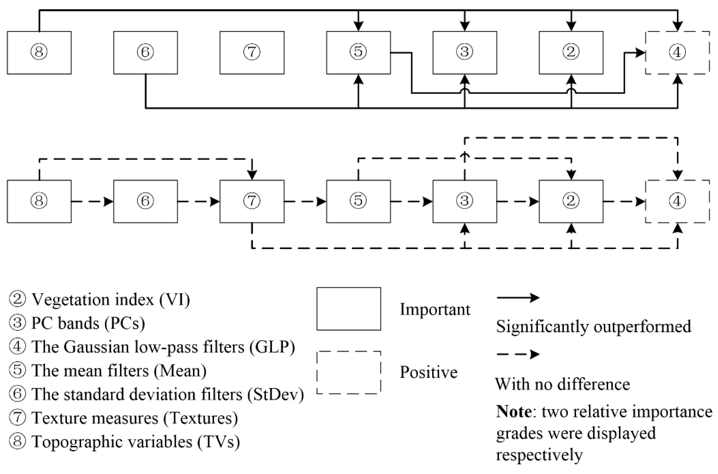
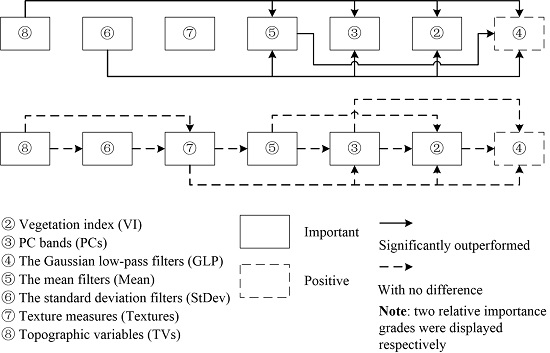
:Land cover classification (LCC) in complex surface-mined landscapes has become very important for understanding the influence of mining activities on the regional geo-environment. There are three characteristics of complex surface-mined areas limiting LCC: significant three-dimensional terrain, strong temporal-spatial variability of surface cover, and spectral-spatial homogeneity. Thus, determining effective feature sets are very important as input dataset to improve detailed extent of classification schemes and classification accuracy. In this study, data such as various feature sets derived from ZiYuan-3 stereo satellite imagery, a feature subset resulting from a feature selection (FS) procedure, training data polygons, and test sample sets were firstly obtained; then, feature sets’ effects on classification accuracy was assessed based on different feature set combination schemes, a FS procedure, and random forest algorithm. The following conclusions were drawn. (1) The importance of feature set could be divided into three grades: the vegetation index (VI), principal component bands (PCs), mean filters (Mean), standard deviation filters (StDev), texture measures (Textures), and topographic variables (TVs) were important; the Gaussian low-pass filters (GLP) was just positive; and none were useless. The descending order of their importance was TVs, StDev, Textures, Mean, PCs, VI, and GLP. (2) TVs and StDev both significantly outperformed VI, PCs, GLP, and Mean; Mean outperformed GLP; all other pairs of feature sets had no difference. In general, the study assessed different feature sets’ effects on LCC in complex surface-mined landscapes.

1. Introduction
Land cover datasets are basic components for global change studies and various applications [1,2]. Currently, researchers are mainly focusing on land cover classification (LCC) at fine scales [3,4,5] in complex landscapes such as agricultural [6,7,8,9], surface-mined land [10,11,12,13,14], and Mediterranean [15] by using high spatial resolution satellite imagery. In general, there are also other landscapes in surface-mined areas, such as agricultural, forest, and cities. Thus, they can be considered as complex surface-mined landscape together for LCC. LCC in surface-mined landscapes (LCCSML) can help with the planning and management of mines.
Classification technology based on machine learning algorithms and high spatial resolution imagery has achieved more accurate results for urban environments, precision agriculture, transportation, forestry surveys, and so on. However, LCCSML differs from other fields in three specific characteristics: significant three-dimensional terrain, strong temporal-spatial variability of surface cover, and spectral-spatial homogeneity. These characteristics increase difficulty of obtaining high accuracy results for the LCCSML [5,14]. As a result, besides powerful classification algorithm, one of the key solutions is to derive beneficial feature sets from helpful satellite sensors. The importance of single features has been examined in our former study [14]. However, the importance of different feature sets for LCCSML has not been investigated.
Some studies attempted to find out the most effective features for classification by assessing the importance of single features. For example, some studies utilized feature selection (FS) procedure as [14], e.g., landslide identification [16,17,18], LCC in arid regions [19], and object-based image analysis LCC [20]. Besides, some others have used different feature combinations by including or excluding specific features for classifications to assess the effects of a single feature, e.g., red-edge band for land-use classification [21]; classifying insect defoliation levels [22]; classification of paddy rice crops [23]; LCC in arid region [19]; and normalized difference vegetation index (NDVI) for classification of tea and hazelnut plantation areas [24].
However, determining effective feature sets is more beneficial than single features. As a result, some studies also used the feature combination method to evaluate the importance of feature sets. For example, Fassnacht et al. [25] aimed to find out which spectral regions were consistently effective for classifying tree species. Akar and Güngör [24] evaluated the contribution of the gray level co-occurrence matrix and Gabor filter texture sets for detecting tea and hazelnut plantation areas. Aguilar et al. [26] grouped different object feature sets such as spectral information, elevation data, band index data and ratios, textures, and shape geometry into 10 strategies for greenhouse extraction and assessed their importance. Wright and Gallant [27] investigated the addition of image texture and digital elevation model-derived terrain variables to Landsat Thematic Mapper variables for wetland discrimination.
Similarly, for agricultural and surface-mined landscapes, Hurni et al. [7] assessed the inclusion of texture measures for the delineation of shifting cultivation landscape. Okubo et al. [8] explored the effectiveness of gray level co-occurrence matrix texture measures for land-use/cover classification in a complex agricultural landscape. Maxwell and Warner [11] investigated the use of multi-temporal terrain data for differentiating mine-reclaimed grasslands from non-mining grasslands. Maxwell et al. [12] assessed RapidEye image- and light detection and ranging (LiDAR)-derived variable sets for geographic object-based image analysis classification of mining and mine reclamation. Maxwell et al. [13] examined the incorporation of LiDAR-derived data for mapping of mining and mine reclamation area by making comparison to data derived by using only RapidEye imagery bands. However, those studies just examined whether the feature sets were effective. There is little research that grades and ranks the importance of feature sets, which might be more beneficial than that of single features for LCCSML. Only few studies have analyzed the relative importance between different feature sets, e.g., the comparison of co-occurrence-, Gabor-, and Markov random fields-based textures for sea-ice classification [28]. Similarly, there is little research that grades the relative importance.
As shown in [14], the random forest (RF) algorithm is easy to implement and can significantly outperform support vector machine and artificial neural network algorithms for the LCCSML. Furthermore, the RF algorithm is known to be less sensitive to the proposed feature set compared to other algorithms, such as support vector machine [14,18]. Thus, using RF to rank and grade importance of feature sets is more reliable than other algorithms.
The objective of this study is to reveal how different feature sets the affect accuracy of LCCSML to rank the importance of feature sets. First, based on our former study [14], the feature sets derived from ZiYuan-3 stereo satellite imagery (ZY-3), the feature subset resulting from a FS procedure, the training data polygons, and the test sample sets were directly obtained. Then, three types of feature set combination schemes were evaluated by combining FS and the RF algorithm.
2. Materials and Methods
2.1. Test Site and Data Set
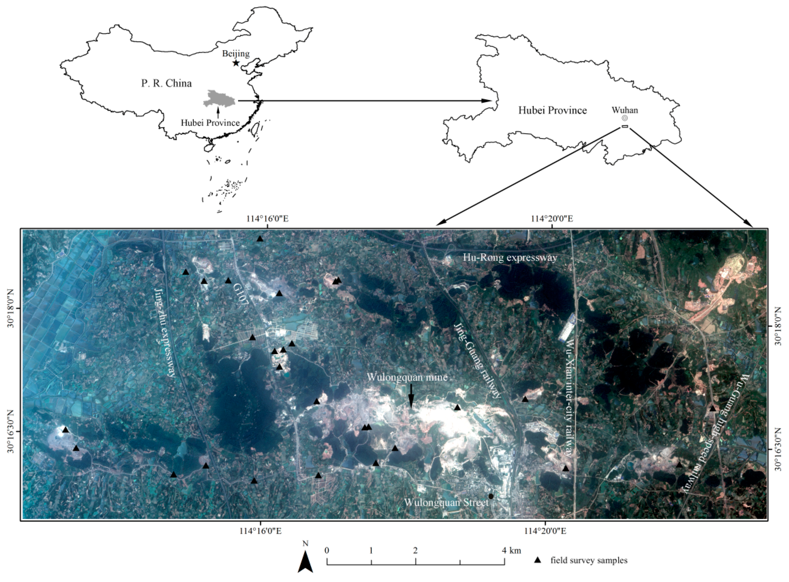
In this study, a test site with area of 109.4 km2 located in Wuhan City of China (114°12′33.59″E–114°23′6.89″E and 30°15′38.85″N–30°18′57.48″N) was selected for the analysis (Figure 1) [14]. Surface mining is prominent features of the test site. The mine disturbance here has a history of nearly 60 years, and most of the mines are active nowadays, especially the Wulongquan mine. The test site also covers a variety of agricultural activities such as crop cultivation (e.g., rice, cotton, corn, rapeseed, and wheat), greenhouse farming, forestry, and aquaculture [14]. The test site is located in the subtropical humid monsoon climate zone, and the annual average temperate is 15.9–17.9 °C. The rainfall is concentrated in the rainy season of early summer with an annual average rainfall amount of about 1347.7 mm. Several national road networks pass through the test site (Figure 1). The locations of the 28 field survey samples are shown in Figure 1, which is the same as our previous research [14].
A ZY-3 stereo satellite image acquired on 20 June 2012, was used in the analysis. ZY-3 is equipped with four cameras, namely, one 2.1 m nadir-looking panchromatic camera, two 3.6 m front- and backward-looking panchromatic cameras, and one 5.8 m nadir-looking multispectral camera. The 3.6 m resolution front and backward looking panchromatic data were used to extract relative digital terrain models (DTM) data with 10 m resolution using ENVI (The Environment for Visualizing Images) 5.0 software. Then, 2.1 m resolution panchromatic–multispectral fused data were generated [14].
2.2. Employed Feature Sets
Our former study [14] used a total of 106 pixel-based features for LCCSML and the importance of single features was assessed. Although there are hundreds of feature sets developed in some other studies, this study further examined the importance of the feature sets formed by those 106 features. The features could be divided into eight types (Table 1): (1) four spectral bands (SBs); (2) one vegetation index (VI): NDVI; (3) two principal component bands (PCs); (4) 12 Gaussian low-pass (GLP) filter features; (5) 12 mean (Mean) filter features; (6) 12 standard deviation (StDev) filter features; (7) 60 texture measures (Textures); and (8) three topographic variables (TVs). The detailed description can be found in our former study [14].
In the former study [14], a feature subset with 34 features for LCCSML was obtained based on the 106 features and a FS method Feature subset, which is used in this study (Table 1). In the feature subset, only the following seven types of features were included: SBs, VI, PCs, GLP, Mean, StDev, and TVs.
2.3. Referenced Data
In this study, the LCC schemes developed in [14] were used. The first-level scheme includes the following seven land cover classes: crop land, forest land, water, road, urban and rural residential land, bare land, and surface-mined land. As explained in [14], 20 second-level land cover classes were further acquired to improve the classification accuracy of the first-level land covers. The components of these land covers were as follows: (1) crop land: paddy field, vegetation and fruit greenhouse, dry land, and fallow land; (2) forest land: woodland, shrub forest, forest under stress, and nursery and orchard; (3) water: pond and stream and mine pit lake; (4) road: black road, white road, and gray road; (5) urban and rural residential land: white roof building, red roof building, and blue roof building; (6) bare land: exposed rock/soil; and (7) surface-mined land: opencast stope, mineral processing land, and dumping site.
The same as in [14], besides the accuracy assessment, the following procedures were based on the second-level land cover classes: training set construction, implementation of feature selection, and classifier training and prediction. The training set that was obtained in [14] by using referenced training data polygons, and a stratified random sampling method was used in this study. The training set involves 40,000 pixels (Figure 2), in which each of the second-level land covers contained 2000 samples. Moreover, the classification results were finally grouped into seven first-level land classes for the accuracy assessments. Accordingly, the test set with 700 pixels (100 in each of the first-level classes) that was acquired in [14] was used in this study (Figure 2). Specifically, the test set was selected by a stratified random sampling method from the classification result that erased the training data polygons. As a result, the test set was independent of the training data polygons.
2.4. Feature Set Combinations and Classification Procedure
Based on the employed feature sets and the training and test sets, three feature combinations were constructed by two feature set combination schemes with FS (named 1, 2, and 3, as listed in Figure 3) to examine the influence of feature sets for LCCSML. A flow chart of the procedure used is shown in Figure 3.
2.4.1. Feature Combinations
In this study, the following three types of feature combinations were constructed (Table 2): (1) Combination 1: SBs and SBs + different types of feature sets, i.e., SBs + VI, SBs + PCs, SBs + GLP, SBs + Mean, SBs + StDev, SBs + Textures, and SBs + TVs; (2) Combination 2: feature subset and feature subset − different types of feature sets, i.e., feature subset − VI, feature subset − PCs, feature subset − GLP, feature subset − Mean, feature subset − StDev, and feature subset − TVs (feature subset involves some features of the six feature sets (Table 1), and here we use the abbreviations of the six feature sets for the convenience of expression; the later analysis will consider this issue), with “−” representing exclusion of certain feature sets from the feature subset, and used similarly hereinafter; and (3) Combination 3: performing FS on SBs + some types of feature sets that have numerous features, i.e., SBs + GLP + FS, SBs + Mean + FS, SBs + StDev + FS, and SBs + Textures + FS. Combinations 1 and 2 were used to determine the importance of feature sets by analyzing the accuracy improvements and losses as a result of their addition or exclusion. Combination 3 was used to further analyze the effects of those four features on LCCSML when using FS.
2.4.2. Feature Selection Procedure
The same as in [14], the varSelRF package [29] in the R platform [30] was utilized with two parameters, namely, 2000 trees for the first forest to produce a feature rank and 500 trees for the subsequent forest to iteratively eliminate the least important features. Finally, the feature combination with the lowest out-of-bag error was considered as the optimal result of FS.
Considering that feature subset often shows data-dependency, this study also used 20 training sets that were obtained in [14] to further produce a final robust feature subset. The use of the random feature selection allows the RF to select the most important features with allowing the diversity among the trees. In particular, based on 20 preliminary feature subsets, this study first ranked the features by selected times, mean ranks, and standard deviation values of ranks as in [14], and, then, explored different thresholds of selected times to determine the final feature subset.
2.4.3. Classification Model Construction and Accuracy Assessment
The RF algorithm [31] is a non-parametric ensemble method based on decision trees. Readers could reference the formulas in [31] and Figure 1 in [32] for further understanding. RF have been reported to be with promising classification capacity in some remote sensing applications [32,33,34,35]. Considering the randomization principle of the RF algorithm, 10 random training sets were used. The training and parameter optimization of the RF algorithm were conducted in the R platform [30] by using the randomForest package [36] and e1071 package [37]. The default value of 500 trees was used for the parameter ntree, and the parameter mtry had to be optimized suggested by [32,38]. Specially, in the process of RF model construction the function “best.tune” of e1071 package called the function “randomForest” of randomForest package with a 10-fold cross-validation method. The parameter value that resulted in highest average overall accuracy in the process of cross-validation was the optimized mtry value, in which the range of mtry was from 1 to the number of features.
Accuracy assessment was conducted by using the test set collected in [14] (Section 2.3). The average F1-measure [39] and overall accuracy were also calculated for each classification. The F1-measure is the harmonic average of the precision and recall, where an F1 score reaches its best value at 1 (perfect precision and recall) and worst at 0. The percentage deviations [21] of F1-measure and overall accuracy were utilized to assess the differences of two different results derived from different feature combinations with FS. Additionally, the McNemar test [40] was used to determine whether the two results had difference that was statistically significant by using the results that have minimal OA differences with the average OA values.
3. Results
Experiment 1 using feature Combination 1 aimed to analyze the effects of the addition of different types of feature sets for LCCSML to assess the importance of feature sets (Section 3.2). The purpose of Experiment 2 using feature Combination 2 was to analyze the effects of the exclusion of different types of feature sets for LCCSML (Section 3.3). Since the feature sets had different size, for example VI, PCs, and TVs had only 1–3 features, the others had 12 features (GLP, Mean, StDev) or 60 features (Textures), it is possible that some feature sets resulted in higher accuracy improvements only due to the larger number of features within the set. As a result, Experiment 3 that based on feature Combination 3 further assessed the importance of feature sets by a FS method to obtain commensurate feature set size (Section 3.4). The results of the FS procedures are shown in Section 3.1.
3.1. Feature Selection Results for SBs Following the Addition of Some Types of Feature Sets
For LCCSML when using SBs and some types of feature sets, i.e., SBs + GLP, SBs + Mean, SBs + StDev, and SBs + Textures, FS was performed, and the preliminary results are shown in Table 3, Table 4, Table 5 and Table 6. Other features that have never been selected in the feature selection process are not listed in these tables. The former study [14] used a selected time threshold of 16 for 20 runs to pick out the final feature subsets, i.e., in which the features were selected by at least 80% of the runs. In view of the results in Table 3, Table 4, Table 5 and Table 6, the features with the selected time of 20 were picked out to form the final feature subsets (bold in tables). As a result, there were 6, 6, 8, and 6 features in the final feature subsets, respectively. It could be concluded that the sizes of SBs + GLP + FS, SBs + Mean + FS, SBs + StDev + FS, and SBs + Textures + FS were commensurate with those of SBs, SBs + VI, SBs + PCs, and SBs + TVs. In general, using the results of feature Combination 3 to assess the effects of those feature sets could achieve more reliable information (for details, see Section 3.4).
3.2. Analysis of the Addition of Different Types of Feature Sets to SBs for LCCSML
3.2.1. Overall Accuracy, F1-Measure, and Percentage Deviation
The average F1-measure and overall accuracy obtained by using SBs and different types of feature sets are shown in Table 7, in which the best results are displayed in bold. The average overall accuracies ranged from 54.8 ± 1.3% (SBs + PCs) to 64.8 ± 1.4% (SBs + TVs). The very low accuracies could be attributed to the difficulty of LCCSML and the insufficiency of effective information provided by only two types of features.
Compared to SBs, by adding different types of feature sets the percentage deviations (%) of average overall accuracies were −0.3%, −1.4%, 3.8%, 9.8%, 14.0%, 10.8%, and 16.5% (Table 7). Table 7 shows that the addition of VI and PCs decreased the overall accuracies. However, the addition of GLP, Mean, StDev, Textures, and TVs contributed to the classifications, and their descending order of importance was TVs, StDev, Textures, Mean, and GLP. Because VI and PCs were linearly computed from spectral bands, their addition imported relevant, even redundant information, which might have led to accuracy losses. Although many studies indicated that the addition of VI contributed to the classification [19,41], some others also supported the conclusion in this study. For example, Adelabu et al. [22] reported that, when using all the bands of RapidEye imagery, adding NDVI decreased the classification accuracy. Conversely, the other feature sets were nonlinear features derived from spectral bands, and these data may have provided some heterogeneous information that improved the classifications.
With regard to the F1-measure of each class, the models with only SBs were better than those with SBs + VI and SBs + PCs with the exception of water and urban and rural residential land. Moreover, the models with the additions of other feature sets did not show consistent trends in terms of the overall accuracies. For example, with respect to crop land, the descending order of F1-measures was the models with the additions of TVs, StDev, Mean, GLP, and Textures. Besides, there were some exceptions, i.e., the F1-measures for some classes decreased: the models with SBs and StDev for water; and the models with SBs and Textures for water. Overall, almost all of the models achieved over 80% F1-measures for water and surface-mined land. However, road and urban and rural residential land achieved only 20–50% F1-measures, and those of the other types were 40–70%.
Besides, each land cover class also showed different percentage deviations in response to the addition of different feature sets. Especially, some percentage deviations were very large: the models of SBs + TVs for crop land (17.2%), the models of SBs + StDev, SBs + Textures, and SBs + TVs for forest land (16.9%, 14.3%, and 19.5%, respectively), and the models of SBs + Mean, SBs + StDev, SBs + Textures, and SBs + TVs for road (23.4%, 72.6%, 63.8%, and 52.8%, respectively) and urban and rural residential land (52.0%, 86.8%, 96.5%, and 48.1%, respectively).
Moreover, it could be drawn that some feature sets were specific to some classes and the feature sets were complementary. For example, the use of Textures led to the best F1-measure values for urban and rural residential land, whereas the use of TVs resulted in the best F1-measure values for crop land, forest land, and water. It might be attributed to that Textures could better discriminate urban and rural residential land from road by better characterizing their shape textures, even if their spectral profiles are similar. The use of DTM allowed to better characterize the elevation for crop land, forest land, and water.
3.2.2. McNemar Test
McNemar test was executed on each pair of classifications derived from SBs with different types of feature sets added. The chi-square values are shown in Table 8, in which the shaded ones larger than 3.84 indicated statistically significant differences at the confidence level of 95% (p < 0.05). The results revealed that: (1) although the addition of VI and PC imported negative effects, they were not statistically significant, i.e., the chi-square values were 0.00 and 0.43, respectively, when compared with the models with only SBs; (2) four of the other five feature sets showed significant positive effects, i.e., the addition of the Mean (8.70), StDev (12.55), Textures (7.67), and TVs (20.90) compared to the models with only SBs; (3) although there were significant differences between the models that added the GLP, Mean, StDev, Textures, and TVs and those that added VI and PC, the results meant little as a result of the negative effects of VI and PC; (4) Mean, StDev, and TVs significantly outperformed GLP, with chi-square values of 4.10, 6.90, and 14.04, respectively; and (5) there were no significant differences among the models that added Mean, StDev, Textures, and TVs.
3.3. Analysis of the Exclusion of Different Types of Feature Sets from Feature Subset for LCCSML
3.3.1. Overall Accuracy, F1-Measure, and Percentage Deviation
The average F1-measure and overall accuracy obtained by excluding different types of feature sets from feature subset are shown in Table 9. The overall accuracies ranged from 77.6% (feature subset) to 66.2 ± 1.0% (feature subset − StDev).
Compared to feature subset, by excluding different types of feature sets, the percentage deviations (%) of overall accuracies were −4.6%, −4.8%, −3.0%, −7.5%, −14.6%, and −11.7% (Table 9). This means that excluding VI, PCs, GLP, Mean, StDev, and TVs decreased the classifications, and their descending order of importance was StDev, TVs, Mean, PCs, VI, and GLP.
In regard to the F1-measure of each class, the models that excluded different types of feature sets from feature subset were nearly almost worse than that with feature subset, with some exceptions: the model with feature subset − VI for bare land and surface-mined land; the model with feature subset − GLP for urban and rural residential land, bare land, and surface-mined land. Overall, all of the models achieved over 80% F1-measures for water and surface-mined land. However, road and urban and rural residential land only achieved approximately 40–70% F1-measures as they were spectrally similar, and those of the other types were approximately 60–80%.
Besides, each land cover class also showed different percentage deviations during the exclusion of different feature sets. In particular, some percentage deviations were very large: the models of feature subset − StDev and feature subset − TVs for crop land (−19.7% and −18.6%), forest land (−12.6% and −11.7%), and bare land (−14.4% and −14.2%); the models of feature subset − Mean, feature subset − StDev, and feature subset − TVs for urban and rural residential land (−12.4%, −28.2%, and −13.1%, respectively); and all models for road (−14.5%, −13.4%, −12.5%, −18.0%, −38.8%, and −22.9%, respectively).
3.3.2. McNemar Test
McNemar test was implemented on each pair of classifications derived from the models with feature subset and feature subset excluding different types of feature sets. The chi-square values are shown in Table 10, in which the shaded ones larger than 3.84 indicated statistically significant differences at the confidence level of 95% (p < 0.05). The results revealed that: (1) excluding the VI, PCs, Mean, StDev, and TVs resulted in significant accuracy decreases with chi-square values of 6.58, 11.64, 13.45, 36.50, and 23.84, respectively; (2) the models with feature subset − StDev and feature subset − TVs significantly outperformed that with feature subset − VI; (3) excluding the StDev and TVs also resulted in significant accuracy losses compared to excluding PCs, and the chi-square values were 13.23 and 4.88; and (4) significant differences were observed between feature subset − Mean and feature subset − GLP (6.70), feature subset − StDev and feature subset − GLP (23.73), feature subset − TVs and feature subset − GLP (12.20), and feature subset − StDev and feature subset − Mean (9.03).
3.4. Analysis of the Addition of Some Types of Feature Sets to SBs with FS for LCCSML
3.4.1. Overall Accuracy, F1-Measure, and Percentage Deviation
The average F1-measure and overall accuracy calculated by the results derived from the models that added some types of feature sets to SBs with FS are shown in Table 11, in which the best results are displayed in bold. The overall accuracies ranged from 58.1 ± 1.1% (SBs + GLP + FS) to 64.5 ± 0.9% (SBs + StDev + FS).
Compared to SBs + GLP, SBs + Mean, SBs + StDev, and SBs + Textures, by performing FS, the percentage deviations (%) of overall accuracies were 0.7%, −1.8%, 1.7%, and −0.5%, respectively (Table 11). After FS, two of the four models’ overall accuracies decreased, i.e., SBs + Mean + FS and SBs + Textures + FS, while the other models improved the classifications.
With regard to the F1-measure of each class, SBs + GLP, SBs + Mean, SBs + StDev, and SBs + Textures were compared with SBs + GLP + FS, SBs + Mean + FS, SBs + StDev + FS, and SBs + Textures + FS, respectively. The models with FS were better than those with SBs + GLP and SBs + StDev, though some exceptions existed: the models with SBs + GLP + FS for water, road, bare land, and surface-mined land; the models with SBs + StDev + FS for water. The models with FS were worse than that with SBs + Mean and SBs + Textures, though exceptions existed: the models with SBs + Mean + FS for forest land and bare land; the models with SBs + Textures + FS for crop land, forest land, water, and surface-mined land. Overall, the four models with FS almost achieved over 80% F1-measures for water and surface-mined land. Similarly, road and urban and rural residential land achieved only 20–50% F1-measures, and those of the other types were 50–70%.
Besides, each land cover class also showed different percentage deviations in response to the addition of FS. The percentage deviation approximately ranged from −4% to 4%, with only three exceptions: the model with SBs + Mean + FS for urban and rural residential land (−16.7%); the model with SBs + Textures + FS for urban and rural residential land (−13.3%) and bare land (−6.9%).
Comparing the average OA values of SBs, SBs + GLP + FS, SBs + Mean + FS, SBs + StDev + FS, SBs + Textures + FS, and SBs + TVs that having commensurate feature set size, it could be concluded that their descending order of importance was TVs, StDev, Textures, Mean, and GLP. This conclusion was more reliable and as same as that drawn in Section 3.2.
3.4.2. McNemar Test
McNemar test was executed on each pair of classifications derived from SBs with the addition of some types of feature sets with FS. The chi-square values after FS are shown in Table 12. The results showed that FS did not significantly improve or reduce the classification accuracies. Besides, the chi-square values for the above-mentioned models with commensurate feature set size are shown in Table 13, in which the shaded ones that larger than 3.84 also indicated statistically significant differences at the confidence level of 95% (p < 0.05). The results revealed that: (1) SBs + Mean + FS, SBs + StDev + FS, and SBs + Textures + FS significantly outperformed SBs; (2) SBs + StDev + FS outperformed SBs + GLP + FS and SBs + Mean + FS; and (3) SBs + TVs outperformed SBs + GLP + FS and SBs + Mean + FS.
4. Discussion
4.1. Assessment of Feature Sets
For assessing the importance of feature sets, the following three grades were defined (Table 14): (1) important, i.e., the feature sets could exert statistically significant effects on LCCSML; (2) positive, i.e., the feature sets could provide effective information for LCCSML but did not result in significant effects; and (3) useless, i.e., the feature sets had little effects on LCCSML. Specifically, when based on SBs, whether the addition of different types of feature sets achieved significant improvements or resulted in no effects should be examined. Similarly, when based on feature subset, whether the exclusion of different types of feature sets achieved significant decreases or resulted in no effects should be investigated. For the relative importance between different feature sets, the following two types were defined (Table 15): (1) significantly outperformed, i.e., one feature set statistically significantly outperformed another feature set; and (2) with no difference, i.e., one feature set resulted in higher accuracy improvement than another feature set but with no statistically significant difference. Specifically, whether SBs + one feature set significantly outperformed SBs + another feature set and whether feature subset − another feature set significantly outperformed feature set − one feature set should be examined.
4.1.1. Importance of Feature Sets
Importance of VI and PCs
As shown in the feature subset in which the importance of single features was indicated [14], VI and PCs could provide effective information for the LCCSML. Specifically, VI had very high importance that was only second to DTM. The first PC band had moderate importance inferior to some features from TVs, VI, Mean, and GLP, and the importance of the second PC band was very low. However, the results obtained in Section 3.2 showed that the addition of VI and PCs slightly decreased the classification accuracy compared to the use of only SBs because of the importing of relevant and even redundant information. Thus, the results in Section 3.2 did not reflect the effects of adding VI and PCs to SBs, and the drawn conclusion was not used to determine the importance grades of VI and PCs. In contrast, the results in Section 3.3 showed that the exclusion of VI and PCs resulted in significant accuracy loss. As a result, it could be concluded that VI and PCs were important (Figure 4).
Importance of GLP, Mean, and StDev
For GLP, Mean, and StDev, some of their features were selected as members of the feature subset, and the results revealed that those feature sets could provide effective information for the LCCSML. The results obtained in Section 3.2 showed that the addition of GLP, Mean, and StDev contributed to the classifications compared to the use of only SBs, and the latter two feature sets resulted in significant improvements. Similarly, the results in Section 3.3 revealed that the exclusion of GLP, Mean, and StDev from feature subset decreased the classification accuracies, and the latter two feature sets resulted in significant reductions. In addition, Section 3.4 indicated that SBs + Mean + FS and SBs + StDev + FS significantly outperformed SBs, and there was slight difference between SBs + Mean + FS and SBs. As a result, it could be concluded that the Mean and StDev were important and the GLP was positive (Figure 4) for the LCCSML.
Importance of Textures and TVs
For the Textures and TVs, only some features from TVs were selected in the feature subset (i.e., TVs could provide effective information for the LCCSML and the effectiveness of Textures was not clear [14]). However, the results presented in Section 3.2 indicated that the addition of Textures and TVs significantly contributed to the classifications compared to the use of only SBs. Similarly, the results in Section 3.3 showed that the exclusion of TVs from the feature subset resulted in significant accuracy loss. Especially, SBs + Textures + FS significantly outperformed SBs (Section 3.4). In other words, it could be concluded that Textures and TVs were important for the LCCSML (Figure 4).
4.1.2. Relative Importance between Different Feature Sets
Relative Importance of VI and PCs
For the relative importance of the VI and PCs, the former study [14] concluded based on the importance of single features that the features from VI outperformed those from PCs. In Section 3.2, the addition of VI and PCs to SBs decreased the classifications as a result of the import of relevant, even redundant information. Therefore, this section could not provide effective information for the judgment of the relative importance of VI and PCs. The results presented in Section 3.3 indicated that PCs was more effective than VI but with no significant difference, i.e., the chi-square value of feature subset − VI and feature subset − PCs was 0.83. In other words, it could be concluded that there was no difference between VI and PCs (Figure 4).
Relative Importance of GLP, Mean, and StDev
For the relative importance of GLP, Mean, and StDev, the former study [14] concluded based on the importance of single features that the features from Mean outperformed those from GLP, and the features from StDev achieved lower importance. However, the results presented in Section 3.2 revealed that StDev had the greatest importance, followed by Mean and GLP (i.e., the overall accuracy of SBs + StDev > that of SBs + Mean > that of SBs + GLP). Especially, Mean and StDev significantly outperformed GLP (with chi-square values of 4.10 and 6.90, respectively), and there was no difference between StDev and Mean (with a chi-square value of 1.31). Similarly, the results presented in Section 3.3 indicated that StDev showed the greatest importance, followed by Mean and GLP (i.e., the overall accuracy of feature subset − StDev < that of feature subset − Mean < that of feature subset − GLP). However, each pair of them was associated with significant differences. Section 3.4 indicated that StDev outperformed GLP and Mean, and there was no difference between Mean and GLP. It seems then that the conclusions drawn above were inconsistent. The importance ranks that derived from single feature importance (i.e., features from Mean > features from GLP > features from StDev) and the experiments with additions of feature sets to SBs (Section 3.2), exclusions of feature sets from feature subset (Section 3.3), and additions of some feature sets to SBs with FS (Section 3.4) (StDev > Mean > GLP) were inconsistent. This inconsistence could be attributed to the fact that the importance of single features did not represent the importance of feature sets. For the GLP, Mean, and StDev, only partial features from them were selected as members of the feature subset according to importance metrics, and the others were deemed to be unimportant according to importance metrics. Especially, the importance rank of the selected features from those three feature sets was disordered. For example, some selected features from Mean were less important than some of those from GLP and StDev. The conclusion drawn from single feature importance was just a general judgment. Therefore, it could be concluded that the descending order of importance was as follows: StDev, Mean, and GLP. As for the statistical significance between them, inconsistencies existed in whether there was a significant difference between StDev and Mean, and Mean and GLP according the results derived in Section 3.2, Section 3.3 and Section 3.4. Considering that SBs and feature subset were the basic feature sets used for comparisons in Section 3.2, Section 3.3 and Section 3.4, and the latter feature set was more effective than the former for the LCCSML, especially StDev in Section 3.3 just involved four features (Table 1), the conclusions from Section 3.3 were adopted when there were small conflicts. In other words, it could be concluded that StDev significantly outperformed Mean and GLP, and Mean also significantly outperformed GLP (Figure 4).
Relative Importance among Those Five Feature Sets
The results in Section 3.3 (see Figure 4) revealed that: (1) VI slightly outperformed GLP (i.e., the overall accuracy of feature subset − VI < that of feature subset − GLP with a chi-square value of 0.58) and PCs slightly outperformed VI (i.e., the overall accuracy of feature subset − PCs < that of feature subset − VI with a chi-square value of 0.38); also PCs slightly outperformed GLP (1.89); (2) Mean slightly outperformed PCs (i.e., the overall accuracy of feature subset − Mean < that of feature subset − PCs with a chi-square value of 0.80) and slightly outperformed VI (i.e., the overall accuracy of feature subset − Mean < that of feature subset − VI with a chi-square value of 2.03); and (3) StDev significantly outperformed VI (i.e., the overall accuracy of feature subset − StDev < that of feature subset − VI with a chi-square value of 17.15) and PCs (i.e., the overall accuracy of feature subset − StDev < that of feature subset − PCs with a chi-square value of 13.23).
Relative Importance of Textures and TVs
For the relative importance of Textures and TVs, the results presented in Section 3.2 showed that TVs slightly outperformed Textures (i.e., the overall accuracy of SBs + TVs > that of SBs + Textures with a chi-square value of 1.85), and similar conclusion was drawn in Section 3.4 (2.59). However, the results presented in Section 3.3 could not provide any additional information. In other words, TVs slightly outperformed Textures (Figure 4).
Others
Moreover, the results obtained in Section 3.2 showed that: (1) StDev slightly outperformed Textures (i.e., the overall accuracy of SBs + StDev > that of SBs + Textures with a chi-square value of 0.94) (Figure 4); (2) Textures slightly outperformed GLP (i.e., the overall accuracy of SBs + Textures > that of SBs + GLP with a chi-square value of 3.53) and Mean (i.e., the overall accuracy of SBs + Textures > that of SBs + Mean with a chi-square value of 0.12) (Figure 4); (3) the relative importance between Textures and VI, and Textures and PCs was not clear (Figure 4), which could be attributed to the fact that the addition of VI and PCs to SBs decreased the classification because of the import of relevant, even redundant information; (4) TVs slightly outperformed StDev (i.e., the overall accuracy of SBs + TVs > that of SBs + StDev with a chi-square value of 0.33); (5) TVs significantly outperformed GLP and slightly outperformed Mean (with the corresponding chi-square values of 14.04 and 3.60); and (6) similarly, the relative importance between TVs and VI, and TVs and PCs was not clear.
Besides, as indicated in Section 3.3: (1) StDev slightly outperformed TVs (i.e., the overall accuracy of feature subset − StDev < that of feature subset − TVs with a chi-square value of 1.04); and (2) TVs significantly outperformed VI, PCs, and GLP (with corresponding chi-square values of 8.31, 4.88, and 12.20), and slightly outperformed Mean (2.56).
Section 3.4 indicated that: (1) TVs significantly outperformed GLP and Mean (with corresponding chi-square values of 11.50 and 5.96), and slightly outperformed StDev and Textures (with corresponding chi-square values of 0.04 and 2.59); (2) StDev slightly outperformed Textures (with corresponding chi-square values of 2.77); and (3) Textures slightly outperformed GLP and Mean (with corresponding chi-square values of 2.52 and 0.49).
The relative importance of StDev and TVs according to the results derived in Section 3.2, Section 3.3 and Section 3.4 was inconsistent. Considering Section 3.2 and Section 3.4 supported that TVs slightly outperformed StDev, especially in Section 3.2 the size of TVs was smaller than that of StDev, the conclusion from Section 3.2 and Section 3.3 was adopted (Figure 4). AS for the relative importance between TVs and the GLP and Mean, Section 3.2 agreed with Section 3.3 that TVs significantly outperformed GLP and slightly outperformed Mean. However, Section 3.4 indicated that TVs significantly outperformed GLP and Mean. Considering the sizes of used features from Mean and TVs were commensurate in Section 3.4, the conclusion from here was adopted (Figure 4). As for the relative importance between TVs and VI, and TVs and PCs, the results in Section 3.2 could not provide any additional information, and significant differences were detected in Section 3.3. Accordingly, TVs significantly outperformed VI and PCs (Figure 4). Because Textures slightly outperformed Mean and GLP, it could be drawn that Textures slightly outperformed VI and PCs.
These conclusions can provide beneficial information for the LCC in various landscapes, for example in agricultural setting, the Mediterranean, the urban fringe, upland forest and so on. In the future, the conclusions would be systematically examined for the LCCSML at fine scale based on object-based image analysis method by integrating more features and feature sets, such as topography variables-derived hydrology and landscape position information [42,43], filter feature sets with larger kernels, and texture sets with different methods and so on.
5. Conclusions
LCCSML was challenging as a result of significant three-dimensional terrain, strong temporal-spatial variability of surface cover, and spectral-spatial homogeneity. One of the key solutions is to derive beneficial feature sets. The importance of single features has been examined in our former study [14]. However, how to determine effective feature sets as input dataset has not been investigated. The present study aimed to reveal that how different feature sets affect accuracy of the LCCSML and assess the importance of feature sets. The feature sets derived from ZY-3 stereo satellite imagery, a feature subset, training data polygons, and test sample sets were firstly obtained; then, three feature set combination schemes were evaluated by combining FS and RF algorithm. In general, the study assessed different feature sets’ effects on LCC in complex surface-mined landscapes. The following conclusions were drawn.
(1) The importance of feature sets was graded. VI, PCs, Mean, StDev, Textures, and TVs were important, i.e., their addition significantly contributed to the accuracies of LCCSML, while GLP was positive, i.e., adding it was effective but did not achieve statistically significant improvement.
(2) The importance of feature sets was ranked and their relative importance was graded. The descending order of the importance of feature sets was TVs, StDev, Textures, Mean, PCs, VI, and GLP. TVs and StDev both significantly outperformed VI, PCs, GLP, and Mean; Mean outperformed GLP; and all other pairs of feature sets had no difference.
Acknowledgments
This research was jointly supported by the Fundamental Research Funds for Central Universities, China University of Geosciences (Wuhan) (Nos. CUGL150417 and CUG170648), the China Geological Survey (No. 12120115063201), Natural Science Foundation of China (No. 41701516), and Hubei Provincial Natural Science Foundation of China (Nos. 2017CFB279 and 2017CFB356).
Author Contributions
All authors made significant contributions to the manuscript. Xianju Li and Weitao Chen conceived of, designed, and performed the experiments and wrote the manuscript. Haixia He and Lizhe Wang helped to analyze the results and revise the manuscript.
Conflicts of Interest
The authors declare no conflict of interest.
References
- Gong, P.; Wang, J.; Yu, L.; Zhao, Y.C.; Zhao, Y.Y.; Liang, L.; Niu, Z.; Huang, X.; Fu, H.; Liu, S.; et al. Finer resolution observation and monitoring of global land cover: First mapping results with Landsat TM and ETM+ data. Int. J. Remote Sens. 2013, 34, 2607–2654. [Google Scholar] [CrossRef]
- Sellers, P.J.; Meeson, B.W.; Hall, F.G.; Asrar, G.; Murphy, R.E.; Schiffer, R.A.; Bretheron, F.P.; Dickinson, R.E.; Ellingson, R.G.; Huemmrich, K.F.; et al. Remote sensing of the land surface for studies of global change: Models—Algorithms—Experiments. Remote Sens. Environ. 1995, 51, 3–26. [Google Scholar] [CrossRef]
- Myint, S.W.; Gober, P.; Brazel, A.; Grossman-Clarke, S.; Weng, Q. Per-pixel vs. object-based classification of urban land cover extraction using high spatial resolution imagery. Remote Sens. Environ. 2011, 115, 1145–1161. [Google Scholar] [CrossRef]
- Senf, C.; Leitão, P.J.; Pflugmacher, D.; van der Linden, S.; Hostert, P. Mapping land cover in complex Mediterranean landscapes using Landsat: Improved classification accuracies from integrating multi-seasonal and synthetic imagery. Remote Sens. Environ. 2015, 156, 527–536. [Google Scholar] [CrossRef]
- Yan, W.Y.; Shaker, A.; El-Ashmawy, N. Urban land cover classification using airborne LiDAR data: A review. Remote Sens. Environ. 2015, 158, 295–310. [Google Scholar] [CrossRef]
- Goodin, D.G.; Anibas, K.L.; Bezymennyi, M. Mapping land cover and land use from object-based classification: An example from a complex agricultural landscape. Int. J. Remote Sens. 2015, 36, 4702–4723. [Google Scholar] [CrossRef]
- Hurni, K.; Hett, C.; Epprecht, M.; Messerli, P.; Heinimann, A. A texture-based land cover classification for the delineation of a shifting cultivation landscape in the Lao PDR using landscape metrics. Remote Sens. 2013, 5, 3377–3396. [Google Scholar] [CrossRef] [Green Version]
- Okubo, S.; Parikesit; Muhamad, D.; Harashina, K.; Takeuchi, K.; Umezaki, M. Land use/cover classification of a complex agricultural landscape using single-dated very high spatial resolution satellite-sensed imagery. Can. J. Remote Sens. 2010, 36, 722–736. [Google Scholar] [CrossRef]
- Piiroinen, R.; Heiskanen, J.; Mõttus, M.; Pellikka, P. Classification of crops across heterogeneous agricultural landscape in Kenya using AisaEAGLE imaging spectroscopy data. Int. J. Appl. Earth Obs. Geoinf. 2015, 39, 1–8. [Google Scholar] [CrossRef]
- Maxwell, A.E.; Strager, M.P.; Warner, T.A.; Zegre, N.P.; Yuill, C.B. Comparison of NAIP orthophotography and RapidEye satellite imagery for mapping of mining and mine reclamation. Gisci. Remote Sens. 2014, 51, 301–320. [Google Scholar] [CrossRef]
- Maxwell, A.E.; Warner, T.A. Differentiating mine-reclaimed grasslands from spectrally similar land cover using terrain variables and object-based machine learning classification. Int. J. Remote Sens. 2015, 36, 4384–4410. [Google Scholar] [CrossRef]
- Maxwell, A.E.; Warner, T.A.; Strager, M.P.; Conley, J.F.; Sharp, A.L. Assessing machine-learning algorithms and image- and lidar-derived variables for GEOBIA classification of mining and mine reclamation. Int. J. Remote Sens. 2015, 36, 954–978. [Google Scholar] [CrossRef]
- Maxwell, A.E.; Warner, T.A.; Strager, M.P.; Pal, M. Combining RapidEye satellite imagery and Lidar for mapping of mining and mine reclamation. Photogram. Eng. Remote Sens. 2014, 80, 179–189. [Google Scholar] [CrossRef]
- Li, X.; Chen, W.; Cheng, X.; Wang, L. A comparison of machine learning algorithms for mapping of complex surface-mined and agricultural landscapes using ZiYuan-3 stereo satellite imagery. Remote Sens. 2016, 8, 514. [Google Scholar] [CrossRef]
- Rodriguez-Galiano, V.F.; Chica-Olmo, M.; Abarca-Hernandez, F.; Atkinson, P.M.; Jeganathan, C. Random forest classification of Mediterranean land cover using multi-seasonal imagery and multi-seasonal texture. Remote Sens. Environ. 2012, 121, 93–107. [Google Scholar] [CrossRef]
- Chen, G.; Li, X.; Chen, W.; Cheng, X.; Zhang, Y.; Liu, S. Extraction and application analysis of landslide influential factors based on LiDar DEM: A case study in the Three Gorges area, China. Nat. Hazards 2014, 74, 509–526. [Google Scholar] [CrossRef]
- Chen, W.; Li, X.; Wang, Y.; Chen, G.; Liu, S. Forested landslide detection using LiDar data and the random forest algorithm: A case study of the Three Gorges, China. Remote Sens. Environ. 2014, 152, 291–301. [Google Scholar] [CrossRef]
- Li, X.; Cheng, X.; Chen, W.; Chen, G.; Liu, S. Identification of forested landslides using LiDar data, object-based image analysis, and machine learning algorithms. Remote Sens. 2015, 7, 9705–9726. [Google Scholar] [CrossRef]
- Li, X.; Chen, W.; Cheng, X.; Liao, Y.; Chen, G. Comparison and integration of feature reduction methods for land cover classification with RapidEye imagery. Multimed. Tools Appl. 2017. [Google Scholar] [CrossRef]
- Duro, D.C.; Franklin, S.E.; Dube, M.G. Multi-scale object-based image analysis and feature selection of multi-sensor Earth Observation imagery using random forests. Int. J. Remote Sens. 2012, 33, 4502–4526. [Google Scholar] [CrossRef]
- Schuster, C.; Förster, M.; Kleinschmit, B. Testing the red edge channel for improving land-use classifications based on high-resolution multi-spectral satellite data. Int. J. Remote Sens. 2012, 33, 5583–5599. [Google Scholar] [CrossRef]
- Adelabu, S.; Mutanga, O.; Adam, E. Evaluating the impact of red-edge band from Rapideye image for classifying insect defoliation levels. ISPRS J. Photogramm. Remote Sens. 2014, 95, 34–41. [Google Scholar] [CrossRef]
- Kim, H.O.; Yeom, J.M. Effect of red-edge and texture features for object-based paddy rice crop classification using RapidEye multi-spectral satellite image data. Int. J. Remote Sens. 2014, 35, 7046–7068. [Google Scholar] [CrossRef]
- Akar, Ö.; Güngör, O. Integrating multiple texture methods and NDVI to the Random Forest classification algorithm to detect tea and hazelnut plantation areas in northeast Turkey. Int. J. Remote Sens. 2015, 36, 442–464. [Google Scholar] [CrossRef]
- Fassnacht, F.E.; Neumann, C.; Förster, M.; Buddenbaum, H.; Ghosh, A.; Clasen, A.; Joshi, P.K.; Koch, B. Comparison of feature reduction algorithms for classifying tree species with hyperspectral data on three central European test sites. IEEE J. Sel. Top. Appl. Earth Obs. Remote Sens. 2014, 7, 2547–2561. [Google Scholar] [CrossRef]
- Aguilar, M.A.; Bianconi, F.; Aguilar, F.J.; Fernández, I. Object-based greenhouse classification from GeoEye-1 and WorldView-2 stereo imagery. Remote Sens. 2014, 6, 3554–3582. [Google Scholar] [CrossRef]
- Wright, C.; Gallant, A. Improved wetland remote sensing in Yellowstone National Park using classification trees to combine TM imagery and ancillary environmental data. Remote Sens. Environ. 2007, 107, 582–605. [Google Scholar] [CrossRef]
- Clausi, D.A. Comparison and fusion of co-occurrence, Gabor and MRF texture features for classification of SAR sea-ice imagery. Atmosphere-Ocean 2001, 39, 183–194. [Google Scholar] [CrossRef]
- Diaz-Uriarte, R. Varselrf: Variable Selection Using Random Forests; R Package Version 0.7-3; TU Wien: Vienna, Austria, 2010. [Google Scholar]
- R Development Core Team. R: A Language and Environment for Statistical Computing; R Foundation for Statistical Computing: Vienna, Austria, 2013. [Google Scholar]
- Breiman, L. Random Forests. Mach. Learn. 2001, 45, 5–32. [Google Scholar] [CrossRef]
- Belgiu, M.; Draguµ, L. Random Forest in remote sensing: A review of applications and future directions. ISPRS J. Photogramm. Remote Sens. 2016, 114, 24–31. [Google Scholar] [CrossRef]
- Pal, M. Random Forest classifier for remote sensing classification. Int. J. Remote Sens. 2005, 26, 217–222. [Google Scholar] [CrossRef]
- Pelletier, C.; Valero, S.; Inglada, J.; Champion, N.; Dedieu, G. Assessing the robustness of Random Forests to map land cover with high resolution satellite image time series over large areas. Remote Sens. Environ. 2016, 187, 156–168. [Google Scholar] [CrossRef]
- Rodríguez-Galiano, V.F.; Ghimire, B.; Rogan, J.; Chica-Olmo, M.; Rigol-Sanchez, J.P. An assessment of the effectiveness of a Random Forest classifier for land-cover classification. ISPRS J. Photogramm. Remote Sens. 2012, 67, 93–104. [Google Scholar] [CrossRef]
- Liaw, A.; Wiener, M. Classification and regression by RandomForest. R News 2002, 2, 18–22. [Google Scholar]
- Meyer, D.; Dimitriadou, E.; Hornik, K.; Weingessel, A.; Leisch, F.; Chang, C.-C.; Lin, C.-C. E1071: Misc Functions of the Department of Statistics (e1071); R Package Version 1.6–4; TU Wien: Vienna, Austria, 2014. [Google Scholar]
- Breiman, L.; Cutler, A. Random Forests Leo Breiman and Adele Cutler—Classification/Clustering—Description. Available online: http://www.stat.berkeley.edu/~breiman/RandomForests/cc_home.htm (accessed on 4 September 2017).
- Daskalaki, S.; Kopanas, I.; Avouris, N. Evaluation of classifiers for an uneven class distribution problem. Appl. Artif. Intell. 2006, 20, 381–417. [Google Scholar] [CrossRef]
- Manandhar, R.; Odeh, I.O.A.; Ancev, T. Improving the accuracy of land use and land cover classification of Landsat data using post-classification enhancement. Remote Sens. 2009, 1, 330–344. [Google Scholar] [CrossRef]
- Li, X.; Chen, G.; Liu, J.; Chen, W.; Cheng, X.; Liao, Y. Effects of RapidEye imagery’s red-edge band and vegetation indices on land cover classification in an arid region. Chin. Geogr. Sci. 2017, 27, 827–835. [Google Scholar] [CrossRef]
- Corcoran, J.; Knight, J.; Gallant, A. Influence of multi-source and multi-temporal remotely sensed and ancillary data on the accuracy of random forest classification of wetlands in northern Minnesota. Remote Sens. 2013, 5, 3212–3238. [Google Scholar] [CrossRef]
- Dannenberg, M.P.; Hakkenberg, C.R.; Song, C. Consistent classification of Landsat time series with an improved automatic adaptive signature generalization algorithm. Remote Sens. 2016, 8, 691. [Google Scholar] [CrossRef]
Figure 1.
Location of the study area and field survey samples, and ZiYuan-3 fused true color image (R, Red; G, Green; B, Blue) [14]. Jing-Zhu expressway: connecting Beijing and Zhuhai; G107: national highway 107 of China; Hu-Rong expressway: connecting Shanghai and Chengdu; Jing-Guang railway: connecting Beijing and Guangzhou; Wu-Xian inter-city railway: connecting Wuhan city and Xianning of Hubei Province, China; Wu-Guang high-speed railway: connecting Wuhan and Guangzhou.

Figure 2.
Location of training and test samples and the red band of ZiYuan-3 fused image.
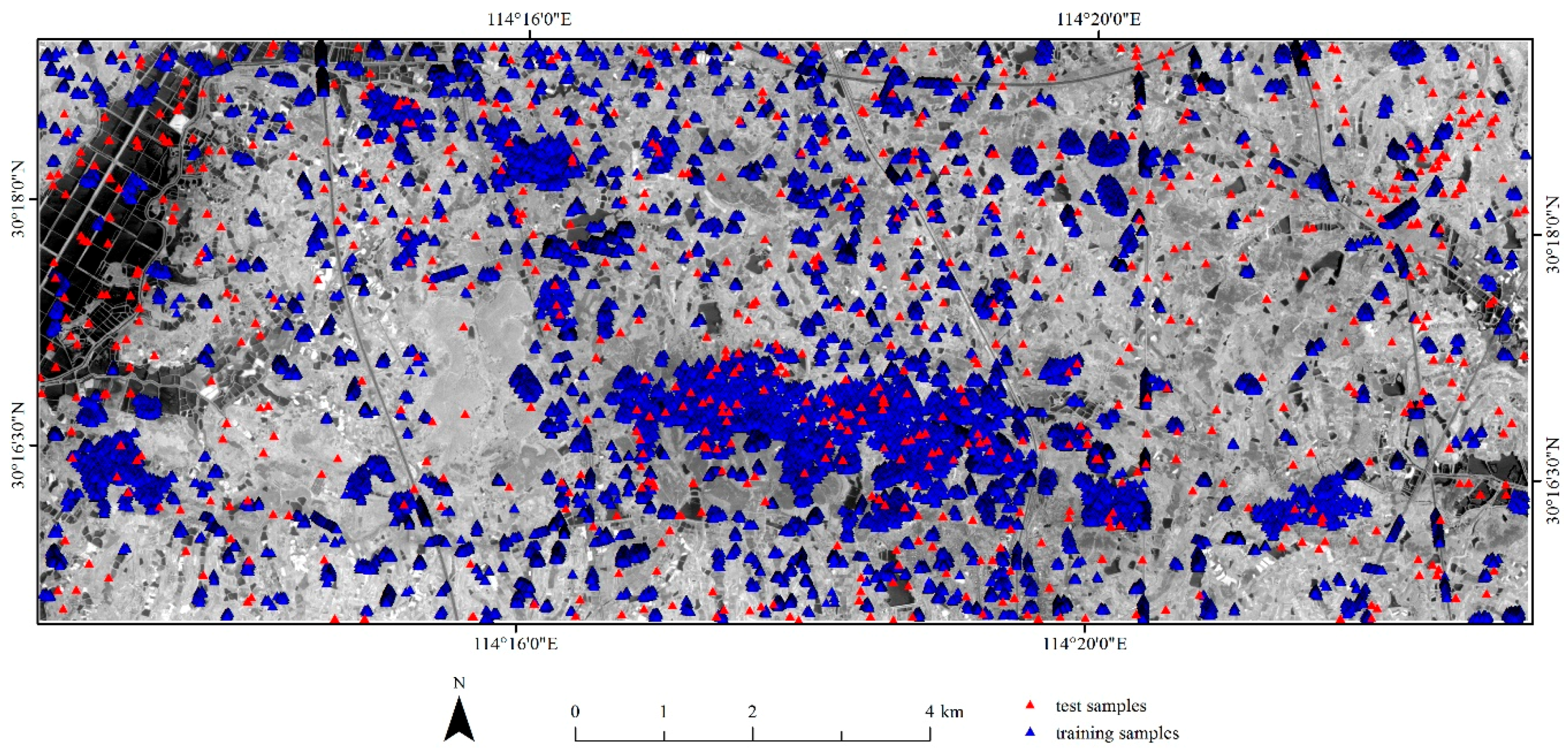
Figure 3.
Flow chart of the feature set combinations and classification procedure.
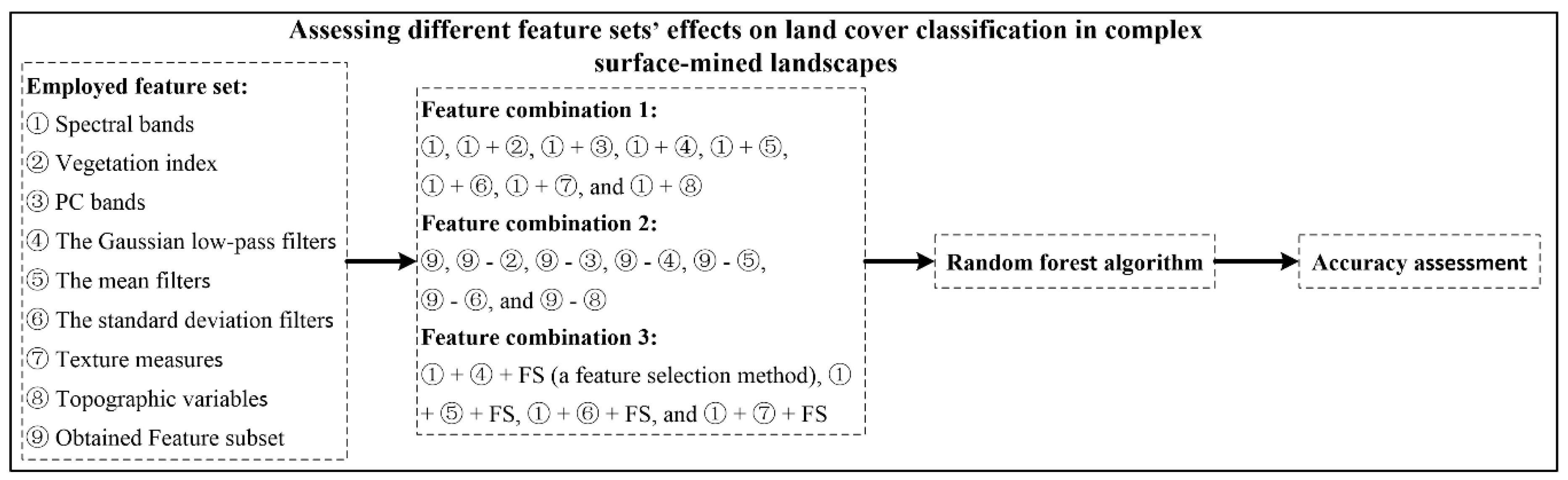
Figure 4.
The importance grade and relative importance of feature sets.

Table 1.
Image feature sets used in this study (revised from [14]). Band (b, g, r, n): the blue, green, red, and near-infrared bands; NDVI: the normalized difference vegetation index; PC: principal component; PC1: the first PC band; PC2: the second PC band; GLP: the Gaussian low-pass filter; Mean: the mean filter; StDev: the standard deviation filter; (3, 5, 7): the three kernel sizes, 3 × 3, 5 × 5, and 7 × 7 pixels; Con, Cor, Asm, Ent, Hom: contrast, correlation, angular second moment, entropy, homogeneity textures; DTM: digital terrain model.
| Image Features | Names | No. | |
|---|---|---|---|
| ① | Spectral bands | Band_(b, g, r, n) | 4 |
| ② | Vegetation index | NDVI | 1 |
| ③ | PC bands | PC1, PC2 | 2 |
| ④ | GLP filter features | GLP_(b, g, r, n)_(3, 5, 7) | 12 |
| ⑤ | Mean filter features | Mean_(b, g, r, n)_(3, 5, 7) | 12 |
| ⑥ | StDev filter features | StDev_(b, g, r, n)_(3, 5, 7) | 12 |
| ⑦ | Texture measures | (Con, Cor, Asm, Ent, Hom)_(b, g, r, n)_(3, 5, 7) | 60 |
| ⑧ | Topographic variables | DTM, slope, aspect | 3 |
| ⑨ | Feature subset | 2 spectral bands (Band_(r,n)), vegetation index (NDVI), PC bands (PC1, PC2), 11 GLP filter features (GLP_(b, g, r, n)_(5, 7), GLP_(b, r, n)_3), Mean filter features (Mean_(b, g, r, n)_(3, 5, 7)), 4 StDev filter features (StDev_(b, g, r)_7, StDev_b_5), and 2 topographic variables (DTM, slope) | 34 |
Table 2.
Feature combinations used in this study: ①: spectral bands; ②: vegetation index; ③: PC bands; ④: the Gaussian low-pass filters; ⑤: the mean filters; ⑥: the standard deviation filters; ⑦: texture measures; ⑧: topographic variables; and ⑨: feature subset. FS: feature selection procedure; -: the number was indefinite. The column titled “No.” in the caption represents the number of different variables. The sign “−” represents exclusion of certain feature sets from the feature subset.
| Combination 1 | No. | Combination 2 | No. | Combination 3 | No. |
|---|---|---|---|---|---|
| ① | 4 | ⑨ | 34 | ① + ④ + FS | - |
| ① + ② | 5 | ⑨ − ② | 33 | ① + ⑤ + FS | - |
| ① + ③ | 6 | ⑨ − ③ | 32 | ① + ⑥ + FS | - |
| ① + ④ | 16 | ⑨ − ④ | 23 | ① + ⑦ + FS | - |
| ① + ⑤ | 16 | ⑨ − ⑤ | 22 | ||
| ① + ⑥ | 16 | ⑨ − ⑥ | 30 | ||
| ① + ⑦ | 64 | ⑨ − ⑧ | 32 | ||
| ① + ⑧ | 7 |
Table 3.
Feature selection results for the spectral bands adding the Gaussian low-pass filters (GLP). _b/g/r/n_3/5/7: the filter features derived from the blue, green, red, and near-infrared bands using the kernel sizes 3 × 3, 5 × 5, and 7 × 7 pixels. Band: the spectral band. The bold features were selected as members of the final feature subset.
| Features | Selected Times | Mean Ranks | Standard Deviation Value of Ranks |
|---|---|---|---|
| GLP_r_7 | 20 | 1.00 | 0.00 |
| GLP_r_5 | 20 | 2.00 | 0.00 |
| GLP_b_7 | 20 | 3.15 | 0.37 |
| GLP_n_7 | 20 | 3.85 | 0.37 |
| GLP_r_3 | 20 | 5.40 | 0.68 |
| GLP_g_7 | 20 | 6.10 | 0.55 |
| GLP_n_5 | 13 | 6.23 | 0.93 |
| Band_r | 13 | 8.00 | 0.00 |
| GLP_n_3 | 13 | 9.00 | 0.00 |
| GLP_b_5 | 13 | 10.08 | 0.28 |
| Band_n | 13 | 11.08 | 0.49 |
| GLP_g_5 | 13 | 11.85 | 0.38 |
| GLP_g_3 | 13 | 13.31 | 0.48 |
| GLP_b_3 | 8 | 13.50 | 0.53 |
| Band_g | 8 | 15.25 | 0.46 |
| Band_b | 8 | 15.75 | 0.46 |
Table 4.
Feature selection results for spectral bands adding the mean filters (Mean). _b/g/r/n_3/5/7: the filter features derived from the blue, green, red, and near-infrared bands using the kernel sizes 3 × 3, 5 × 5, and 7 × 7 pixels. The bold features were selected as members of the final feature subset.
| Features | Selected Times | Mean Ranks | Standard Deviation Value of Ranks |
|---|---|---|---|
| Mean_r_7 | 20 | 1.00 | 0.00 |
| Mean_r_5 | 20 | 2.00 | 0.00 |
| Mean_b_7 | 20 | 3.00 | 0.00 |
| Mean_r_3 | 20 | 4.00 | 0.00 |
| Mean_g_7 | 20 | 5.00 | 0.00 |
| Mean_n_7 | 20 | 6.00 | 0.00 |
| Mean_n_5 | 14 | 7.14 | 0.53 |
| Mean_n_3 | 14 | 8.36 | 0.50 |
| Mean_b_5 | 14 | 8.50 | 0.65 |
| Mean_g_5 | 14 | 10.00 | 0.00 |
Table 5.
Feature selection results for spectral bands adding the standard deviation filter (StDev). Band: the spectral band. _b/g/r/n_5/7: the filter features derived from the blue, green, red, and near-infrared bands using the kernel sizes 5 × 5 and 7 × 7 pixels. The bold features were selected as members of the final feature subset.
| Features | Selected Times | Mean Ranks | Standard Deviation Value of Ranks |
|---|---|---|---|
| Band_n | 20 | 1.00 | 0.00 |
| Band_r | 20 | 2.00 | 0.00 |
| Band_g | 20 | 3.00 | 0.00 |
| Band_b | 20 | 4.00 | 0.00 |
| StDev_b_7 | 20 | 5.40 | 0.50 |
| StDev_r_7 | 20 | 5.60 | 0.50 |
| StDev_g_7 | 20 | 7.00 | 0.00 |
| StDev_n_7 | 20 | 8.75 | 0.44 |
| StDev_b_5 | 15 | 8.00 | 0.00 |
| StDev_r_5 | 12 | 10.00 | 0.00 |
| StDev_n_5 | 3 | 10.00 | 0.00 |
Table 6.
Feature selection result for spectral bands adding the texture measures. Band: the spectral band. _b/g/r/n_7: the texture features derived from the blue, green, red, and near-infrared bands using the kernel size 7 × 7 pixels. Con: contrast texture. Hom: homogeneity texture. The bold features were selected as members of the final feature subset.
| Features | Selected Times | Mean Ranks | Standard Deviation Value of Ranks |
|---|---|---|---|
| Band_n | 20 | 1 | 0 |
| Band_r | 20 | 2 | 0 |
| Band_g | 20 | 3 | 0 |
| Band_b | 20 | 4 | 0 |
| Con_r_7 | 20 | 5 | 0 |
| Con_b_7 | 20 | 6 | 0 |
| Con_g_7 | 1 | 7 | 0 |
| Con_n_7 | 1 | 8 | 0 |
| Hom_r_7 | 1 | 9 | 0 |
Table 7.
The F1-measure and overall accuracy (OA) (%) for land cover classification in complex surface-mined landscapes using spectral bands and different types of feature sets: ①: spectral bands; ②: vegetation index; ③: PC bands; ④: the Gaussian low-pass filters; ⑤: the mean filters; ⑥: the standard deviation filters; ⑦: texture measures; and ⑧: topographic variables. The bold values represent the best F1-measures and OA values. The accuracies with standard deviation were averaged on 10 runs.
| ① | ① + ② | ① + ③ | ① + ④ | ① + ⑤ | ① + ⑥ | ① + ⑦ | ① + ⑧ | |
|---|---|---|---|---|---|---|---|---|
| Crop land | 48.5 ± 2.0 | 48.0 ± 2.6 | 47.4 ± 1.6 | 50.9 ± 3.0 | 52.3 ± 2.3 | 52.5 ± 2.5 | 50.9 ± 1.8 | 56.8 ± 2.0 |
| Forest land | 58.1 ± 2.6 | 57.9 ± 1.9 | 57.9 ± 2.5 | 60.0 ± 2.0 | 62.9 ± 2.3 | 67.9 ± 1.7 | 66.4 ± 2.0 | 69.4 ± 1.9 |
| Water | 86.5 ± 0.6 | 86.9 ± 1.0 | 86.6 ± 1.4 | 86.8 ± 1.0 | 86.7 ± 1.3 | 85.7 ± 1.8 | 82.9 ± 1.3 | 90.4 ± 0.7 |
| Road | 28.0 ± 2.6 | 27.4 ± 2.5 | 26.5 ± 2.9 | 30.4 ± 2.2 | 34.6 ± 2.0 | 48.3 ± 1.9 | 45.9 ± 1.7 | 42.8 ± 3.6 |
| Urban and rural residential land | 27.2 ± 4.9 | 27.3 ± 3.8 | 26.1 ± 5.8 | 28.4 ± 2.8 | 41.3 ± 2.9 | 50.8 ± 2.5 | 53.4 ± 2.1 | 40.3 ± 4.3 |
| Bare land | 55.7 ± 2.1 | 54.4 ± 3.3 | 53.2 ± 2.0 | 57.9 ± 2.9 | 58.9 ± 2.7 | 60.8 ± 3.1 | 58.2 ± 2.2 | 60.4± 2.1 |
| Surface-mined land | 76.4 ± 2.9 | 76.0 ± 1.3 | 75.8 ± 2.7 | 78.6 ± 1.3 | 83.1 ± 2.5 | 80.0 ± 1.0 | 76.6 ± 1.6 | 81.4 ± 2.3 |
| OA | 55.6 ± 1.2 | 55.4 ± 1.0 | 54.8 ± 1.3 | 57.7 ± 1.0 | 61.0 ± 1.3 | 63.4 ± 1.0 | 61.6 ± 0.7 | 64.8 ± 1.4 |
Table 8.
The chi-square values of McNemar tests for land cover classification in complex surface-mined landscapes using spectral bands and different types of feature sets: ①: spectral bands; ②: vegetation index; ③: PC bands; ④: the Gaussian low-pass filters; ⑤: the mean filters; ⑥: the standard deviation filters; ⑦: texture measures; and ⑧: topographic variables. The shaded ones that larger than 3.84 indicated statistically significant differences at the confidence level of 95% (p < 0.05).
| ① + ② | ① + ③ | ① + ④ | ① + ⑤ | ① + ⑥ | ① + ⑦ | ① + ⑧ | |
|---|---|---|---|---|---|---|---|
| ① | 0.00 | 0.43 | 1.74 | 8.70 | 12.55 | 7.67 | 20.90 |
| ① + ② | 0.52 | 2.14 | 10.17 | 13.69 | 8.68 | 24.38 | |
| ① + ③ | 4.17 | 11.57 | 17.01 | 11.16 | 28.16 | ||
| ① + ④ | 4.10 | 6.90 | 3.53 | 14.04 | |||
| ① + ⑤ | 1.31 | 0.12 | 3.60 | ||||
| ① + ⑥ | 0.94 | 0.33 | |||||
| ① + ⑦ | 1.85 |
Table 9.
The F1-measure and overall accuracy (OA) (%) for land cover classification in surface-mined landscapes that involved the exclusion of different types of feature sets from feature subset (⑨): ①: spectral bands; ②: vegetation index; ③: PC bands; ④: the Gaussian low-pass filters; ⑤: the mean filters; ⑥: the standard deviation filters; and ⑧: topographic variables. The sign “−” represents exclusion of certain feature sets from the feature subset. The bold values represent the best F1-measures and OA values. The accuracies with standard deviation were averaged on 10 runs.
| ⑨ | ⑨ − ② | ⑨ − ③ | ⑨ − ④ | ⑨ − ⑤ | ⑨ − ⑥ | ⑨ − ⑧ | |
|---|---|---|---|---|---|---|---|
| Crop land | 74.0 | 69.2 ± 2.5 | 68.8 ± 5.9 | 70.7 ± 2.3 | 66.7 ± 2.5 | 59.4 ± 1.0 | 60.2 ± 1.9 |
| Forest land | 79.8 | 74.5 ± 3.2 | 75.9 ± 4.2 | 76.6 ± 3.2 | 73.4 ± 2.1 | 69.8 ± 1.9 | 70.4 ± 1.3 |
| Water | 91.2 | 88.9 ± 1.4 | 89.7 ± 1.3 | 89.2 ± 0.6 | 90.5 ± 1.3 | 87.8 ± 1.4 | 88.1 ± 1.2 |
| Road | 70.5 | 60.3 ± 1.9 | 61.1 ± 9.3 | 61.7 ± 1.8 | 57.9 ± 3.2 | 43.2 ± 3.1 | 54.4 ± 3.6 |
| Urban and rural residential land | 63.0 | 60.6 ± 1.9 | 59.6 ± 6.6 | 63.2 ± 2.1 | 55.2 ± 2.3 | 45.2 ± 3.4 | 56.6 ± 2.9 |
| Bare land | 76.2 | 76.6 ± 2.0 | 73.5 ± 5.5 | 77.7 ± 1.7 | 72.4 ± 2.9 | 65.3 ± 2.3 | 65.4 ± 2.3 |
| Surface-mined land | 86.9 | 88.0 ± 2.0 | 86.5 ± 1.8 | 87.7 ± 1.4 | 85.7 ± 1.4 | 83.5 ± 1.4 | 83.8 ± 1.9 |
| OA | 77.6 | 74.0 ± 0.9 | 73.8 ± 4.3 | 75.3 ± 1.1 | 71.8 ± 1.4 | 66.2 ± 1.0 | 68.5 ± 0.8 |
Table 10.
The chi-square values of McNemar tests for land cover classification in surface-mined landscapes that involved the exclusion of different types of feature sets from feature subset (⑨): ①: spectral bands; ②: vegetation index; ③: PC bands; ④: the Gaussian low-pass filters; ⑤: the mean filters; ⑥: the standard deviation filters; and ⑧: topographic variables. The sign “−” represents exclusion of certain feature sets from the feature subset. The shaded ones that larger than 3.84 indicated statistically significant differences at the confidence level of 95% (p < 0.05).
| ⑨ − ② | ⑨ − ③ | ⑨ − ④ | ⑨ − ⑤ | ⑨ − ⑥ | ⑨ − ⑧ | |
|---|---|---|---|---|---|---|
| ⑨ | 6.58 | 11.64 | 3.04 | 13.45 | 36.50 | 23.84 |
| ⑨ − ② | 0.38 | 0.58 | 2.03 | 17.15 | 8.31 | |
| ⑨ − ③ | 1.89 | 0.80 | 13.23 | 4.88 | ||
| ⑨ − ④ | 6.70 | 23.73 | 12.20 | |||
| ⑨ − ⑤ | 9.03 | 2.56 | ||||
| ⑨ − ⑥ | 1.04 |
Table 11.
The F1-measure and overall accuracy (OA) (%) for land cover classification in complex surface-mined landscapes using SBs and some types of feature sets with feature selection (FS): ①: spectral bands; ④: the Gaussian low-pass filters; ⑤: the mean filters; ⑥: the standard deviation filters; and ⑦: texture measures. The bold values represent the best F1-measures and OA values. The accuracies with standard deviation were averaged on 10 runs.
| ① + ④ + FS | ① + ⑤ + FS | ① + ⑥ + FS | ① + ⑦ + FS | |
|---|---|---|---|---|
| Crop land | 52.3 ± 1.5 | 51.8 ± 2.0 | 54.6 ± 2.3 | 52.1 ± 2.4 |
| Forest land | 61.3 ± 2.0 | 64.2 ± 1.4 | 67.4 ± 1.9 | 68.3 ± 1.2 |
| Water | 86.6 ± 0.8 | 84.8 ± 1.4 | 86.7 ± 1.4 | 84.2 ± 1.4 |
| Road | 29.9 ± 3.2 | 33.3 ± 1.7 | 50.6 ± 2.9 | 44.0 ± 1.9 |
| Urban and rural residential land | 29.0± 4.3 | 34.4 ± 1.6 | 52.3 ± 2.6 | 46.4 ± 3.4 |
| Bare land | 57.0 ± 3.5 | 61.1 ± 2.5 | 59.9 ± 2.3 | 54.2 ± 3.4 |
| Surface-mined land | 77.6 ± 1.2 | 81.3 ± 3.1 | 80.6 ± 1.2 | 79.5 ± 2.5 |
| OA | 58.1 ± 1.1 | 59.9 ± 0.8 | 64.5 ± 0.9 | 61.3 ± 0.8 |
Table 12.
The chi-square values of McNemar tests for land cover classification in complex surface-mined landscapes using spectral bands and some types of feature sets with feature selection: ①: spectral bands; ④: the Gaussian low-pass filters; ⑤: the mean filters; ⑥: the standard deviation filters; and ⑦: texture measures.
| ① + ④ + FS | ① + ⑤ + FS | ① + ⑥ + FS | ① + ⑦ + FS | |
|---|---|---|---|---|
| ① + ④ | 0.10 | |||
| ① + ⑤ | 0.62 | |||
| ① + ⑥ | 0.27 | |||
| ① + ⑦ | 0.06 |
Table 13.
The chi-square values of McNemar tests for land cover classification in complex surface-mined landscapes using the superior models that involved the addition of some types of feature sets to spectral bands combined with feature selection: ①: spectral bands; ④: the Gaussian low-pass filters; ⑤: the mean filters; ⑥: the standard deviation filters; and ⑦: texture measures. FS80: feature selection with a threshold of 16. FS60: feature selection with a threshold of 12. The shaded ones that larger than 3.84 indicated statistically significant differences at the confidence level of 95% (p < 0.05).
| ① + ④ + FS | ① + ⑤ + FS | ① + ⑥ + FS | ① + ⑦ + FS | ① + ⑧ | |
|---|---|---|---|---|---|
| ① | 2.31 | 5.56 | 16.69 | 8.00 | |
| ① + ④ + FS | 1.01 | 8.60 | 2.52 | 11.50 | |
| ① + ⑤ + FS | 4.64 | 0.49 | 5.96 | ||
| ① + ⑥ + FS | 2.77 | 0.04 | |||
| ① + ⑦ + FS | 2.59 |
Table 14.
Descriptions of the three defined importance grades of feature sets in this study.
| NO. | Grade | Description |
|---|---|---|
| 1 | Important | The feature sets could exert statistically significant effects on LCCSML |
| 2 | Positive | The feature sets could provide effective information for the LCCSML but did not result in significant effects |
| 3 | Useless | The feature sets had little effects on LCCSML |
Table 15.
Descriptions of the two defined relative importance grades between different feature sets in this study.
Table 15.
Descriptions of the two defined relative importance grades between different feature sets in this study.
| NO. | Type | Description |
|---|---|---|
| 1 | Significantly outperformed | One feature set statistically significantly outperformed another feature set. |
| 2 | With no difference | One feature set resulted in higher accuracy improvement than another feature set but with no statistically significant difference. |
© 2017 by the authors. Licensee MDPI, Basel, Switzerland. This article is an open access article distributed under the terms and conditions of the Creative Commons Attribution (CC BY) license (http://creativecommons.org/licenses/by/4.0/).
Share and Cite
MDPI and ACS Style
Chen, W.; Li, X.; He, H.; Wang, L. Assessing Different Feature Sets’ Effects on Land Cover Classification in Complex Surface-Mined Landscapes by ZiYuan-3 Satellite Imagery. Remote Sens. 2018, 10, 23. https://doi.org/10.3390/rs10010023
AMA Style
Chen W, Li X, He H, Wang L. Assessing Different Feature Sets’ Effects on Land Cover Classification in Complex Surface-Mined Landscapes by ZiYuan-3 Satellite Imagery. Remote Sensing. 2018; 10(1):23. https://doi.org/10.3390/rs10010023
Chicago/Turabian StyleChen, Weitao, Xianju Li, Haixia He, and Lizhe Wang. 2018. "Assessing Different Feature Sets’ Effects on Land Cover Classification in Complex Surface-Mined Landscapes by ZiYuan-3 Satellite Imagery" Remote Sensing 10, no. 1: 23. https://doi.org/10.3390/rs10010023
Note that from the first issue of 2016, this journal uses article numbers instead of page numbers. See further details here.