Soil Moisture Mapping from Satellites: An Intercomparison of SMAP, SMOS, FY3B, AMSR2, and ESA CCI over Two Dense Network Regions at Different Spatial Scales

 , ,
, ,  , , and
Abstract
:
1. Introduction
2. Data
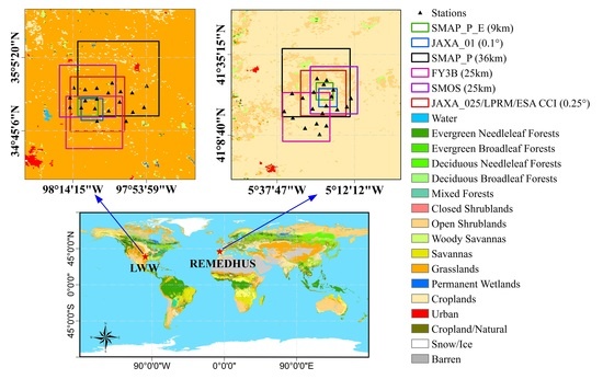
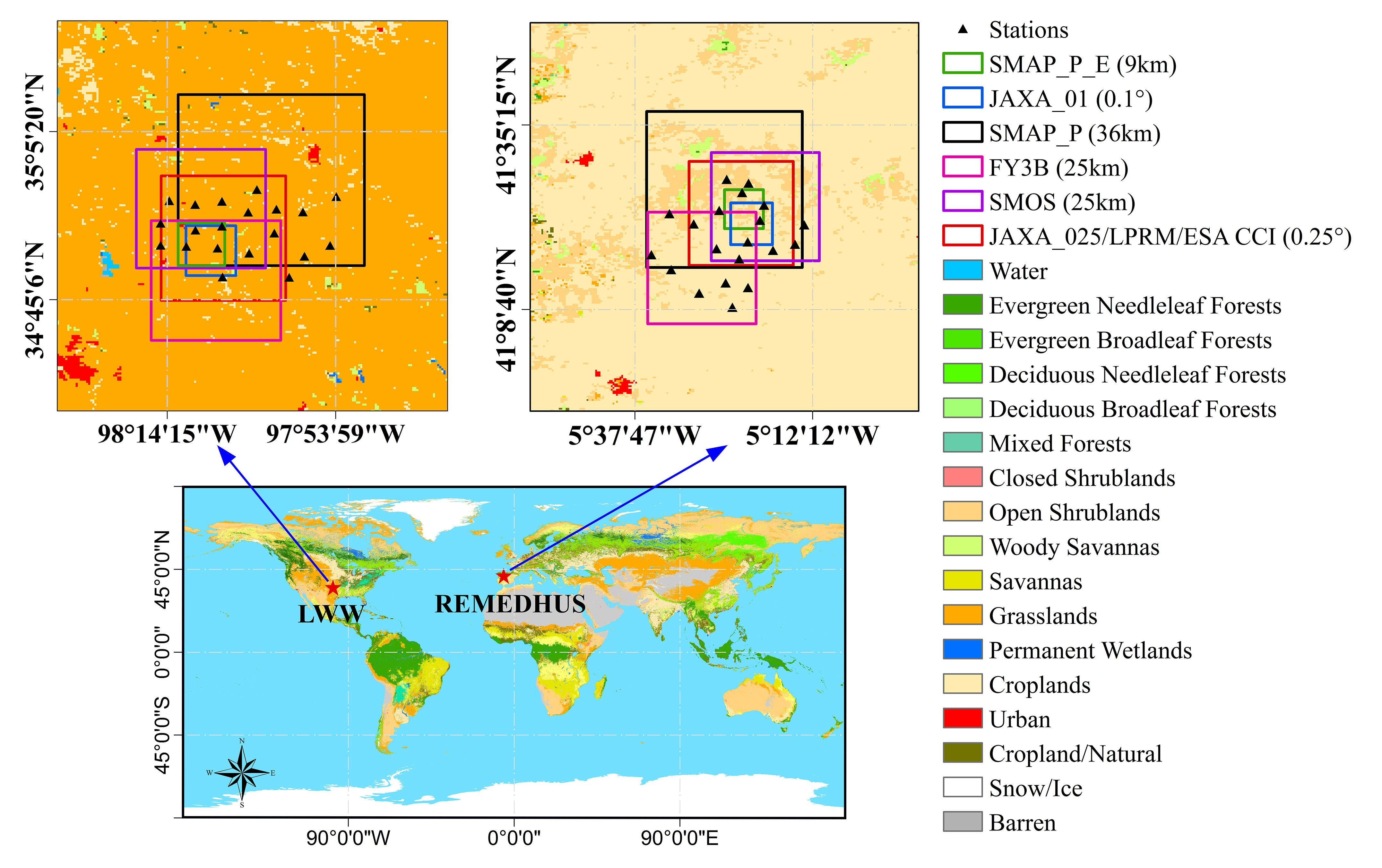
2.1. Study Area and In-Situ Soil Moisture Data
- (1)
- LWW Network: The LWW network was built between Chickasha and Lawton, and is situated within the Great Plains region of the United States, with an area of 611 km2. Currently, it consists of 20 stations, which measure soil moisture at 5, 25, and 45 cm below the surface and soil temperature at 5, 10, 15, 25, 30, and 45 cm in 5-min intervals. The climate of this region is sub-humid, with a stable annual precipitation of 760 mm. The LWW area is moderately rolling, with elevations ranging from 300 m to 500 m, and is mainly covered by grassland, with a wide range of soil textures from fine sand to silty loam. The LWW network has been widely used for monitoring hydrological and meteorological measurements since 1961. It has been extensively used for assessing satellite soil moisture products, due to the large dynamic range of soil moisture and flat terrain in this region [20,21,23,31].
- (2)
- REMEDHUS Network: The REMEDHUS network is a dense network in Spain, which is located in the central semiarid sector of the Duero Basin, with an area of 1300 km2. It is composed of 20 stations that measure soil moisture and surface temperature at 5 cm in 60-min intervals. These data are collected and updated continuously via the International Soil Moisture Network (ISMN) [32]. Croplands and shrublands dominate the land cover of this region. The land usage of the REMEDHUS network region is covered by cereals (78%), forest and pasture (13%), irrigated crops (5%), and vineyards (3%) [30]. The elevation of this region ranges from 700 to 900 m above sea level, with a continental semiarid Mediterranean climate, which brings dry and warm summers and cool and wet winters to this region [33,34]. The mean annual rainfall and average temperature of this region are 385 mm and 12 °C, respectively. The REMEDHUS network has a long history of hydrological-related applications, including the validation of satellite soil moisture products [30,35], the evaluation of soil moisture downscaling algorithm [36,37], and parameterization of water balance models [38].
2.2. Satellite Soil Moisture Products
2.2.1. SMAP Passive and Enhanced Passive Soil Moisture Products
2.2.2. FY3B Soil Moisture Product
2.2.3. SMOS Soil Moisture Product
2.2.4. AMSR2 Soil Moisture Products
2.2.5. ESA CCI Soil Moisture Product
3. Methods
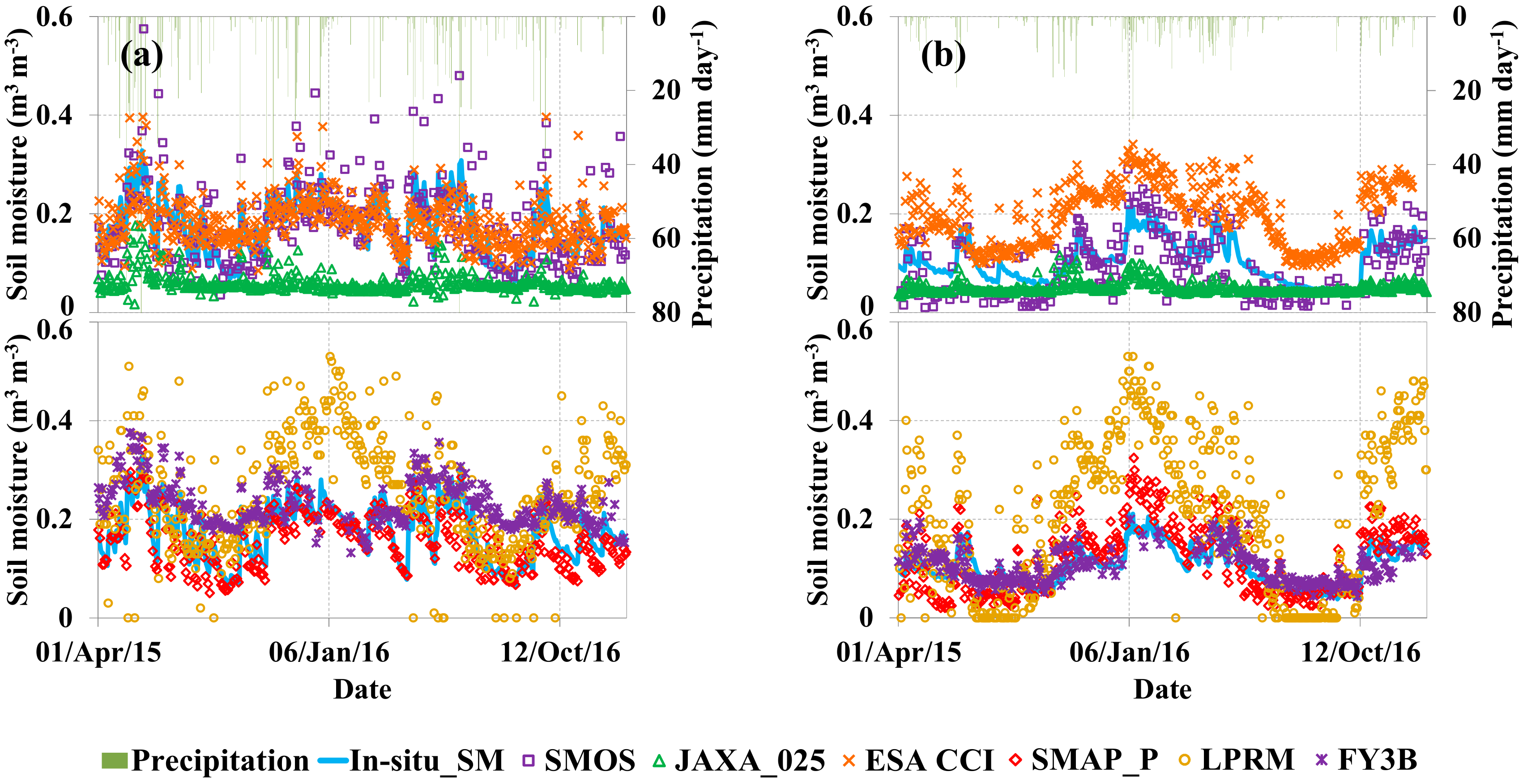
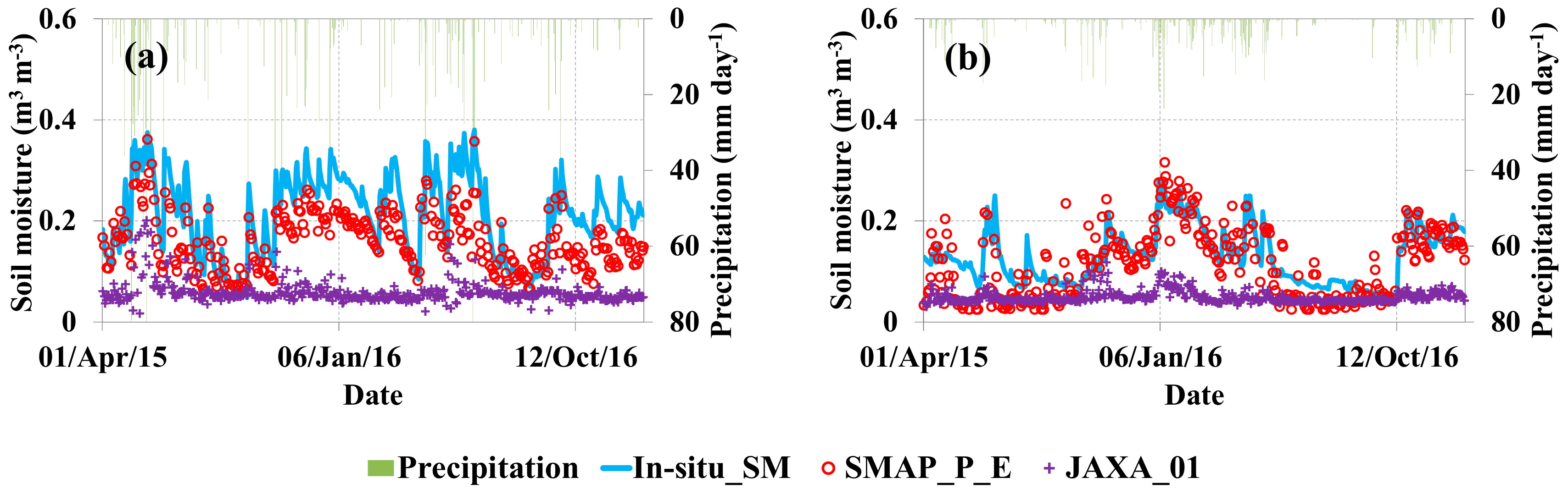
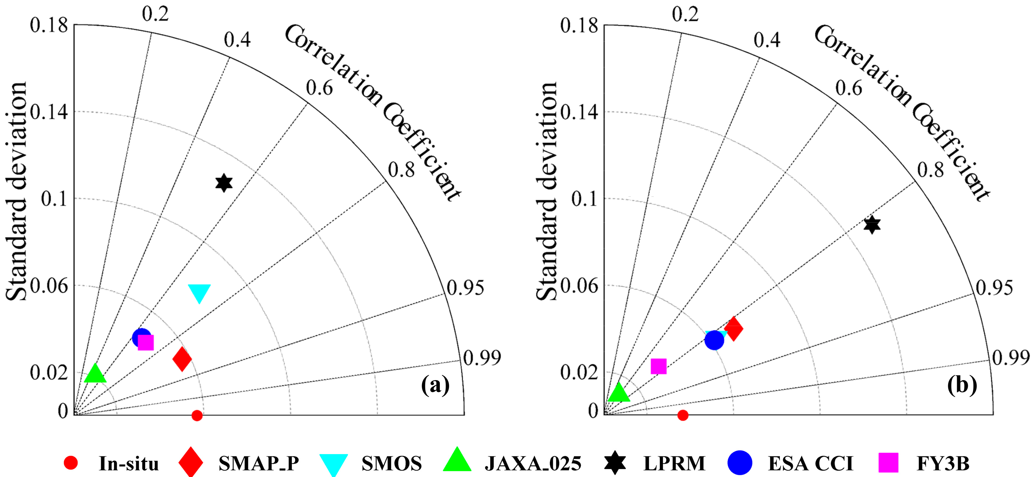
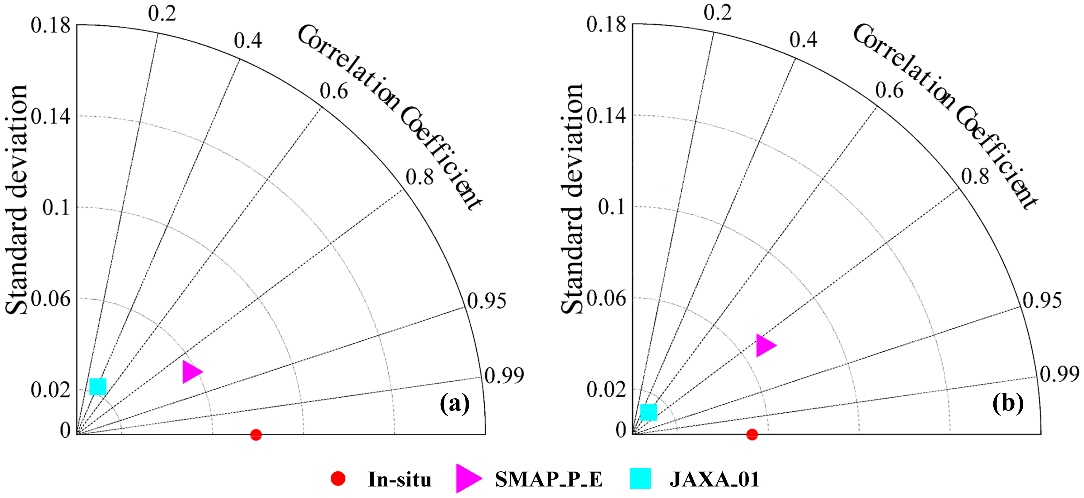
4. Results
5. Discussion
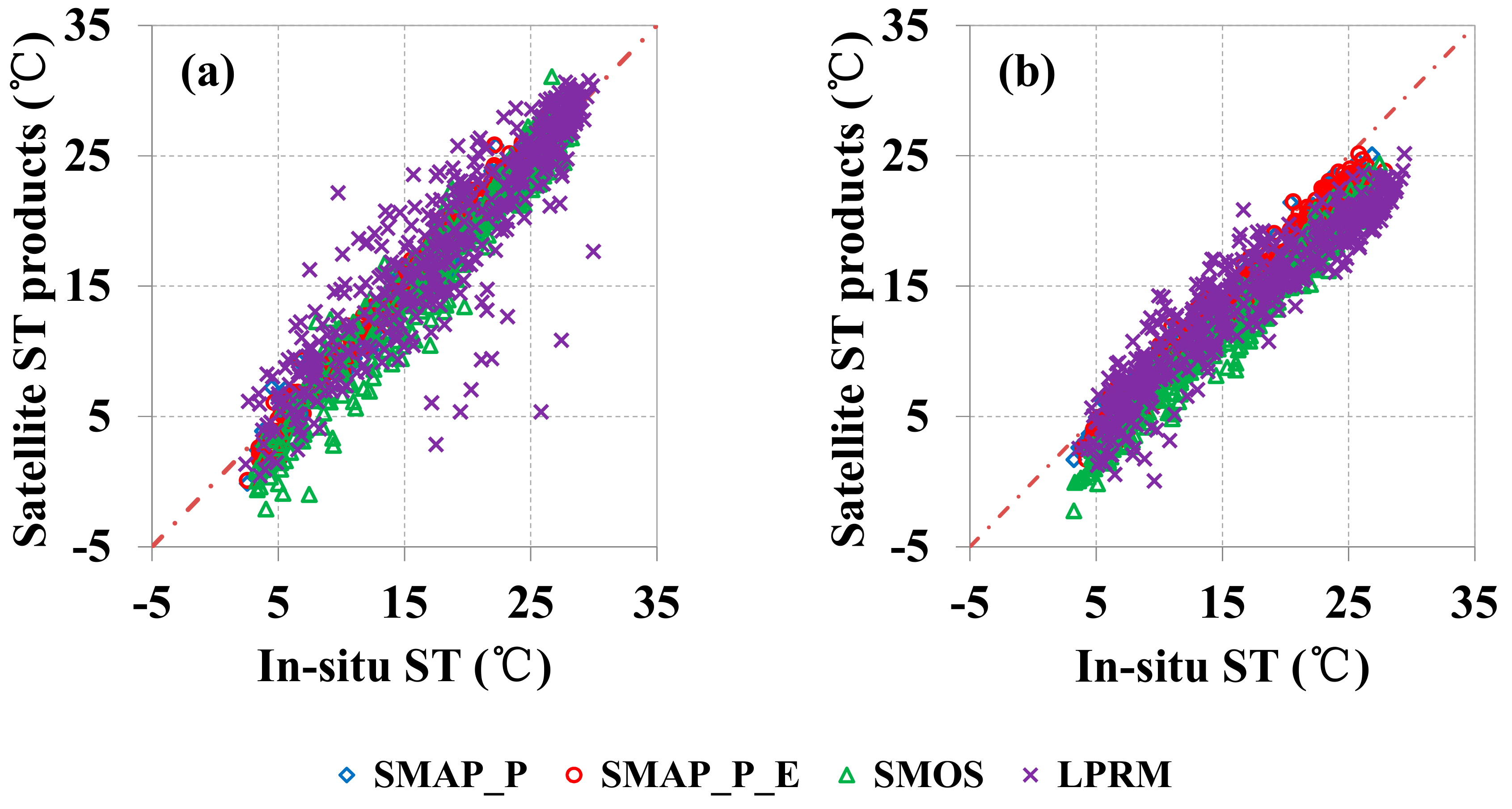
5.1. Assessment of Satellite Surface Temperature Data
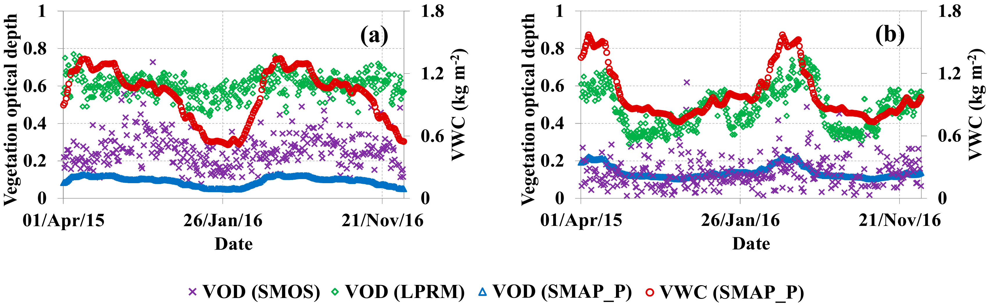
5.2. Temporal Behavior of Satellite Vegetation Optical Depth
6. Conclusions
Acknowledgments
Author Contributions
Conflicts of Interest
References
- Wagner, W.; Hahn, S.; Kidd, R.; Melzer, T.; Bartalis, Z.; Hasenauer, S.; Figa-Saldaña, J.; De Rosnay, P.; Jann, A.; Schneider, S.; et al. The ASCAT soil moisture product: A review of its specifications, validation results, and emerging applications. Meteorol. Z. 2013, 22, 5–33. [Google Scholar] [CrossRef]
- Njoku, E.G.; Jackson, T.J.; Lakshmi, V.; Chan, T.K.; Nghiem, S.V. Soil moisture retrieval from AMSR-E. IEEE Trans. Geosci. Remote Sens. 2003, 41, 215–229. [Google Scholar] [CrossRef]
- Imaoka, K.; Maeda, T.; Kachi, M.; Kasahara, M.; Ito, N.; Nakagawa, K. Status of AMSR2 instrument on GCOM-W1. Proc. SPIE 2012, 8528, 852815. [Google Scholar] [CrossRef]
- Kerr, Y.H.; Waldteufel, P.; Wigneron, J.P.; Delwart, S.; Cabot, F.; Boutin, J.; Escorihuela, M.J.; Font, J.; Reul, N.; Gruhier, C.; et al. The SMOS mission: New tool for monitoring key elements of the global water cycle. Proc. IEEE 2010, 98, 666–687. [Google Scholar] [CrossRef] [Green Version]
- Entekhabi, D.; Njoku, E.G.; O’Neill, P.E.; Kellogg, K.H.; Crow, W.T.; Edelstein, W.N.; Entin, J.K.; Goodman, S.D.; Jackson, T.J.; Johnson, J.; et al. The soil moisture active passive (SMAP) mission. Proc. IEEE 2010, 98, 704–716. [Google Scholar] [CrossRef]
- Wagner, W.; Lemoine, G.; Rott, H. A method for estimating soil moisture from ERS scatterometer and soil data. Remote Sens. Environ. 1999, 70, 191–207. [Google Scholar] [CrossRef]
- Wigneron, J.P.; Jackson, T.J.; O’neill, P.; De Lannoy, G.; De Rosnay, P.; Walker, J.P.; Ferrazzoli, P.; Mironov, V.; Bircher, S.; Grant, J.P.; et al. Modelling the passive microwave signature from land surfaces: A review of recent results and application to the L-band SMOS & SMAP soil moisture retrieval algorithms. Remote Sens. Environ. 2017, 192, 238–262. [Google Scholar]
- Naeimi, V.; Scipal, K.; Bartalis, Z.; Hasenauer, S.; Wagner, W. An improved soil moisture retrieval algorithm for ERS and METOP scatterometer observations. IEEE Trans. Geosci. Remote Sens. 2009, 47, 1999–2013. [Google Scholar] [CrossRef]
- Kerr, Y.H.; Waldteufel, P.; Richaume, P.; Wigneron, J.P.; Ferrazzoli, P.; Mahmoodi, A.; Bitar, A.A.; Cabot, F.; Gruhier, C.; Juglea, S.E.; et al. The SMOS soil moisture retrieval algorithm. IEEE Trans. Geosci. Remote Sens. 2012, 50, 1384–1403. [Google Scholar] [CrossRef]
- Zeng, J.; Li, Z.; Chen, Q.; Bi, H. Method for soil moisture and surface temperature estimation in the Tibetan Plateau using spaceborne radiometer observations. IEEE Geosci. Remote Sens. Lett. 2015, 12, 97–101. [Google Scholar] [CrossRef]
- Jackson, T.J., III. Measuring surface soil moisture using passive microwave remote sensing. Hydrol. Process. 1993, 7, 139–152. [Google Scholar] [CrossRef]
- Owe, M.; de Jeu, R.; Holmes, T. Multisensor historical climatology of satellite-derived global land surface moisture. J. Geophys. Res. Earth Surf. 2008, 113. [Google Scholar] [CrossRef] [Green Version]
- Yang, J.; Zhang, P.; Lu, N.; Yang, Z.; Shi, J.; Dong, C. Improvements on global meteorological observations from the current Fengyun 3 satellites and beyond. Int. J. Digit. Earth 2012, 5, 251–265. [Google Scholar] [CrossRef]
- Dorigo, W.; Wagner, W.; Albergel, C.; Albrecht, F.; Balsamo, G.; Brocca, L.; Chung, D.; Ertl, M.; Forkel, M.; Gruber, A.; et al. ESA CCI Soil Moisture for improved Earth system understanding: State-of-the art and future directions. Remote Sens. Environ. 2017, 203, 185–215. [Google Scholar] [CrossRef]
- Parinussa, R.M.; Wang, G.; Holmes, T.R.H.; Liu, Y.Y.; Dolman, A.J.; De Jeu, R.A.M.; Jiang, T.; Zhang, P.; Shi, J. Global surface soil moisture from the Microwave Radiation Imager onboard the Fengyun-3B satellite. Int. J. Remote Sens. 2014, 35, 7007–7029. [Google Scholar] [CrossRef]
- Zeng, J.; Li, Z.; Chen, Q.; Bi, H.; Qiu, J.; Zou, P. Evaluation of remotely sensed and reanalysis soil moisture products over the Tibetan Plateau using in-situ observations. Remote Sens. Environ. 2015, 163, 91–110. [Google Scholar] [CrossRef]
- Montzka, C.; Bogena, H.R.; Zreda, M.; Monerris, A.; Morrison, R.; Muddu, S.; Vereecken, H. Validation of spaceborne and modelled surface soil moisture products with cosmic-ray neutron probes. Remote Sens. 2017, 9, 103. [Google Scholar] [CrossRef]
- Albergel, C.; De Rosnay, P.; Gruhier, C.; Muñoz-Sabater, J.; Hasenauer, S.; Isaksen, L.; Kerr, Y.; Wagner, W. Evaluation of remotely sensed and modelled soil moisture products using global ground-based in-situ observations. Remote Sens. Environ. 2012, 118, 215–226. [Google Scholar] [CrossRef]
- Su, Z.; Wen, J.; Dente, L.; Velde, R.; Wang, L.; Ma, Y.; Yang, K.; Hu, Z. The Tibetan Plateau observatory of plateau scale soil moisture and soil temperature (Tibet-Obs) for quantifying uncertainties in coarse resolution satellite and model products. Hydrol. Earth Syst. Sci. 2011, 15, 2303–2316. [Google Scholar] [CrossRef]
- Jackson, T.J.; Cosh, M.H.; Bindlish, R.; Starks, P.J.; Bosch, D.D.; Seyfried, M.; Goodrich, D.C.; Moran, M.S.; Du, J. Validation of advanced microwave scanning radiometer soil moisture products. IEEE Trans. Geosci. Remote Sens. 2010, 48, 4256–4272. [Google Scholar] [CrossRef]
- Jackson, T.J.; Bindlish, R.; Cosh, M.H.; Zhao, T.; Starks, P.J.; Bosch, D.D.; Seyfried, M.; Moran, M.S.; Goodrich, D.C.; Kerr, Y.H.; et al. Validation of Soil Moisture and Ocean Salinity (SMOS) soil moisture over watershed networks in the US. IEEE Trans. Geosci. Remote Sens. 2012, 50, 1530–1543. [Google Scholar] [CrossRef] [Green Version]
- Al-Yaari, A.; Wigneron, J.P.; Ducharne, A.; Kerr, Y.; De Rosnay, P.; De Jeu, R.; Govind, A.; Al Bitar, A.; Albergel, C.; Muñoz-Sabater, J.; et al. Global-scale evaluation of two satellite-based passive microwave soil moisture datasets (SMOS and AMSR-E) with respect to Land Data Assimilation System estimates. Remote Sens. Environ. 2014, 149, 181–195. [Google Scholar] [CrossRef] [Green Version]
- Zeng, J.; Chen, K.S.; Bi, H.; Chen, Q. A preliminary evaluation of the SMAP radiometer soil moisture product over United States and Europe using ground-based measurements. IEEE Trans. Geosci. Remote Sens. 2016, 54, 4929–4940. [Google Scholar] [CrossRef]
- Chan, S.K.; Bindlish, R.; O’Neill, P.E.; Njoku, E.; Jackson, T.; Colliander, A.; Chen, F.; Burgin, M.; Dunbar, S.; Piepmeier, J.; et al. Assessment of the SMAP passive soil moisture product. IEEE Trans. Geosci. Remote Sens. 2016, 54, 4994–5007. [Google Scholar] [CrossRef]
- Colliander, A.; Jackson, T.J.; Bindlish, R.; Chan, S.; Das, N.; Kim, S.B.; Cosh, M.H.; Dunbar, R.S.; Dang, L.; Pashaian, L.; et al. Validation of SMAP surface soil moisture products with core validation sites. Remote Sens. Environ. 2017, 191, 215–231. [Google Scholar] [CrossRef]
- Anam, R.; Chishtie, F.; Ghuffar, S.; Qazi, W.; Shahis, I. Inter-comparison of SMOS and AMSR-E soil moisture products during flood years (2010–2011) over Pakistan. Eur. J. Remote Sens. 2017, 50, 442–451. [Google Scholar] [CrossRef]
- Zhuo, L.; Han, D. Hydrological evaluation of satellite soil moisture data in two basins of different climate and vegetation density conditions. Adv. Meteorol. 2017. [Google Scholar] [CrossRef]
- Ray, R.L.; Fares, A.; He, Y.; Temimi, M. Evaluation and Inter-comparison of satellite soil moisture products using in situ observations over Texas. Water 2017, 9, 372. [Google Scholar] [CrossRef]
- Jackson, T.J.; Le Vine, D.M.; Hsu, A.Y.; Oldak, A.; Starks, P.J.; Swift, C.T.; Isham, J.D.; Haken, M. Soil moisture mapping at regional scales using microwave radiometry: The Southern Great Plains Hydrology Experiment. IEEE Trans. Geosci. Remote Sens. 1999, 37, 2136–2151. [Google Scholar] [CrossRef]
- Sanchez, N.; Martínez-Fernández, J.; Scaini, A.; Perez-Gutierrez, C. Validation of the SMOS L2 soil moisture data in the REMEDHUS network (Spain). IEEE Trans. Geosci. Remote Sens. 2012, 50, 1602–1611. [Google Scholar] [CrossRef]
- Kornelsen, K.C.; Cosh, M.H.; Coulibaly, P. Potential of bias correction for downscaling passive microwave and soil moisture data. J. Geophys. Res. 2015, 120, 6460–6479. [Google Scholar] [CrossRef]
- Dorigo, W.A.; Wagner, W.; Hohensinn, R.; Hahn, S.; Paulik, C.; Xaver, A.; Gruber, A.; Drusch, M.; Mecklenburg, S.; Van Oevelen, P.; et al. The International Soil Moisture Network: A data hosting facility for global in-situ soil moisture measurements. Hydrol. Earth Syst. Sci. 2011, 15, 1675–1698. [Google Scholar] [CrossRef]
- Castro, J.; Zamora, R.; Hódar, J.A.; Gómez, J.M. Seedling establishment of a boreal tree species (Pinus sylvestris) at its southernmost distribution limit: Consequences of being in a marginal Mediterranean habitat. J. Ecol. 2004, 92, 266–277. [Google Scholar] [CrossRef]
- Ceballos, A.; Martı́nez-Fernández, J.; Luengo-Ugidos, M.Á. Analysis of rainfall trends and dry periods on a pluviometric gradient representative of Mediterranean climate in the Duero Basin, Spain. J. Arid Environ. 2004, 58, 215–233. [Google Scholar] [CrossRef]
- Wagner, W.; Pathe, C.; Doubkova, M.; Sabel, D.; Bartsch, A.; Hasenauer, S.; Blöschl, G.; Scipal, K.; Martínez-Fernández, J.; Löw, A. Temporal stability of soil moisture and radar backscatter observed by the Advanced Synthetic Aperture Radar (ASAR). Sensors 2008, 8, 1174–1197. [Google Scholar] [CrossRef] [PubMed] [Green Version]
- Piles, M.; Sánchez, N.; Vall-llossera, M.; Camps, A.; Martínez-Fernández, J.; Martínez, J.; González-Gambau, V. A downscaling approach for SMOS land observations: Evaluation of high-resolution soil moisture maps over the Iberian Peninsula. IEEE J. Sel. Top. Appl. Earth Obs. 2014, 7, 3845–3857. [Google Scholar] [CrossRef]
- Sánchez-Ruiz, S.; Piles, M.; Sánchez, N.; Martínez-Fernández, J.; Vall-llossera, M.; Camps, A. Combining SMOS with visible and near/shortwave/thermal infrared satellite data for high resolution soil moisture estimates. J. Hydrol. 2014, 516, 273–283. [Google Scholar] [CrossRef]
- Sánchez, N.; Martínez-Fernández, J.; Calera, A.; Torres, E.; Pérez-Gutiérrez, C. Combining remote sensing and in-situ soil moisture data for the application and validation of a distributed water balance model (HIDROMORE). Agric. Water Manag. 2010, 98, 69–78. [Google Scholar] [CrossRef]
- Choudhury, B.J.; Schmugge, T.J.; Chang, A.; Newton, R.W. Effect of surface roughness on the microwave emission from soils. J. Geophys. Res. Oceans 1979, 84, 5699–5706. [Google Scholar] [CrossRef]
- Mironov, V.L.; Kosolapova, L.G.; Fomin, S.V. Physically and mineralogically based spectroscopic dielectric model for moist soils. IEEE Trans. Geosci. Remote Sens. 2009, 47, 2059–2070. [Google Scholar] [CrossRef]
- O’Neill, P.E.; Chan, S.; Njoku, E.; Jackson, T.J.; Bindlish, R. Algorithm Theoretical Basis Document (ATBD): L2/3_SM_P, Nat. Aeronaut. Space Admin; Jet Propulsion Lab.: Pasadena, CA, USA, 2015. [Google Scholar]
- Chaubell, J.; Yueh, S.; Entekhabi, D.; Peng, J. Resolution enhancement of SMAP radiometer data using the Backus Gilbert optimum interpolation technique. In Proceedings of the 2016 IEEE International Geoscience and Remote Sensing Symposium, Beijing, China, 10–15 July 2016; pp. 284–287. [Google Scholar]
- Poe, G.A. Optimum interpolation of imaging microwave radiometer data. IEEE Trans. Geosci. Remote Sens. 1990, 28, 800–810. [Google Scholar] [CrossRef]
- Chan, S. Enhanced Level 3 Passive Soil Moisture Product Specification Document; Jet Propulsion Lab., California Inst. Technol.: Pasadena, CA, USA, 2016. [Google Scholar]
- De Jeu, R.A.M. Retrieval of Land Surface Parameters Using Passive Microwave Remote Sensing. Ph.D. Thesis, Vrije Universiteit Amsterdam, Amsterdam, The Netherlands, 2003. [Google Scholar]
- Jackson, T.J.; Schmugge, T.J. Vegetation effects on the microwave emission of soils. Remote Sens. Environ. 1991, 36, 203–212. [Google Scholar] [CrossRef]
- Shi, J.; Jiang, L.; Zhang, L.; Chen, K.S.; Wigneron, J.P.; Chanzy, A. A parameterized multifrequency-polarization surface emission model. IEEE Trans. Geosci. Remote Sens. 2005, 43, 2831–2841. [Google Scholar]
- Zeng, J.; Chen, K.S.; Bi, H.; Zhao, T.; Yang, X. A comprehensive analysis of rough soil surface scattering and emission predicted by AIEM with comparison to numerical simulations and experimental measurements. IEEE Trans. Geosci. Remote Sens. 2017, 55, 1696–1708. [Google Scholar] [CrossRef]
- Shi, J.; Jiang, L.; Zhang, L.; Chen, K.S.; Wigneron, J.P.; Chanzy, A.; Jackson, T.J. Physically based estimation of bare-surface soil moisture with the passive radiometers. IEEE Trans. Geosci. Remote Sens. 2006, 44, 3145–3153. [Google Scholar] [CrossRef]
- Wigneron, J.P.; Kerr, Y.; Waldteufel, P.; Saleh, K.; Escorihuela, M.J.; Richaume, P.; Ferrazzoli, P.; De Rosnay, P.; Gurney, R.; Calvet, J.C.; et al. L-band microwave emission of the biosphere (L-MEB) model: Description and calibration against experimental data sets over crop fields. Remote Sens. Environ. 2007, 107, 639–655. [Google Scholar] [CrossRef]
- Lievens, H.; Tomer, S.K.; Al Bitar, A.; De Lannoy, G.J.M.; Drusch, M.; Dumedah, G.; Hendricks Franssen, H.J.; Kerr, Y.H.; Martens, B.; Pan, M.; et al. SMOS soil moisture assimilation for improved hydrologic simulation in the Murray Darling Basin, Australia. Remote Sens. Environ. 2015, 168, 146–162. [Google Scholar] [CrossRef] [Green Version]
- Koike, T.; Nakamura, Y.; Kaihotsu, I.; Davaa, G.; Matsuura, N.; Tamagawa, K.; Fujii, H. Development of an advanced microwave scanning radiometer (AMSR-E) algorithm for soil moisture and vegetation water content. J. Hydraul. Eng. ASCE 2004, 48, 217–222. [Google Scholar] [CrossRef]
- Holmes, T.R.H.; De Jeu, R.A.M.; Owe, M.; Dolman, A.J. Land surface temperature from Ka band (37 GHz) passive microwave observations. J. Geophys. Res. Atmos. 2009, 114. [Google Scholar] [CrossRef] [Green Version]
- Li, L.; Njoku, E.G.; Im, E.; Chang, P.S.; Germain, K.S. A preliminary survey of radio-frequency interference over the US in Aqua AMSR-E data. IEEE Trans. Geosci. Remote Sens. 2004, 42, 380–390. [Google Scholar] [CrossRef]
- Njoku, E.G.; Ashcroft, P.; Chan, T.K.; Li, L. Global survey and statistics of radio-frequency interference in AMSR-E land observations. IEEE Trans. Geosci. Remote Sens. 2005, 43, 938–947. [Google Scholar] [CrossRef]
- Liu, Y.Y.; Dorigo, W.A.; Parinussa, R.M.; De Jeu, R.A.M.; Wagner, W.; McCabe, M.F.; Evans, J.P.; Van Dijk, A.I.J.M. Trend-preserving blending of passive and active microwave soil moisture retrievals. Remote Sens. Environ. 2012, 123, 280–297. [Google Scholar] [CrossRef]
- Kim, H.; Parinussa, R.; Konings, A.; Wagner, W.; Cosh, M.; Choi, M. Global-scale assessment and combination of SMAP with ASCAT (active) and AMSR2 (passive) soil moisture products. Remote Sens. Environ. 2017. [Google Scholar] [CrossRef]
- Rüdiger, C.; Calvet, J.C.; Gruhier, C.; Holmes, T.R.; De Jeu, R.A.M.; Wagner, W. An intercomparison of ERS-Scat and AMSR-E soil moisture observations with model simulations over France. J. Hydrometeorol. 2009, 10, 431–447. [Google Scholar] [CrossRef]
- Entekhabi, D.; Reichle, R.H.; Koster, R.D.; Crow, W.T. Performance metrics for soil moisture retrievals and application requirements. J. Hydrometeorol. 2010, 11, 832–840. [Google Scholar] [CrossRef]
- Taylor, K.E. Summarizing multiple aspects of model performance in a single diagram. J. Geophys. Res. Atmos. 2001, 106, 7183–7192. [Google Scholar] [CrossRef]
- Yee, M.S.; Walker, J.P.; Rüdiger, C.; Parinussa, R.M.; Koike, T.; Kerr, Y. H. A comparison of SMOS and AMSR2 soil moisture using representative sites of the OzNet monitoring network. Remote Sens. Environ. 2017, 195, 297–312. [Google Scholar] [CrossRef]


| Resolution | Products | ubRMSE (m3 m−3) | RMSE (m3 m−3) | Bias (m3 m−3) | R | N |
|---|---|---|---|---|---|---|
| 0.25° | SMAP passive | 0.027 | 0.032 | −0.018 | 0.89 | 311 |
| SMOS | 0.057 | 0.057 | −0.004 | 0.71 | 328 | |
| FY3B | 0.041 | 0.078 | 0.067 | 0.71 | 311 | |
| JAXA | 0.050 | 0.125 | −0.114 | 0.48 | 478 | |
| LPRM | 0.108 | 0.141 | 0.091 | 0.54 | 464 | |
| ESA CCI | 0.044 | 0.045 | 0.009 | 0.66 | 585 | |
| 0.1° | SMAP enhanced passive | 0.040 | 0.064 | −0.050 | 0.88 | 312 |
| JAXA | 0.073 | 0.168 | −0.151 | 0.41 | 468 |
| Resolution | Products | ubRMSE (m3 m−3) | RMSE (m3 m−3) | Bias (m3 m−3) | R | N |
|---|---|---|---|---|---|---|
| 0.25° | SMAP passive | 0.044 | 0.047 | 0.016 | 0.83 | 348 |
| SMOS | 0.038 | 0.040 | −0.012 | 0.83 | 236 | |
| FY3B | 0.025 | 0.027 | 0.009 | 0.75 | 325 | |
| JAXA | 0.035 | 0.065 | −0.055 | 0.60 | 538 | |
| LPRM | 0.121 | 0.161 | 0.106 | 0.82 | 518 | |
| ESA CCI | 0.036 | 0.104 | 0.097 | 0.83 | 464 | |
| 0.1° | SMAP enhanced passive | 0.039 | 0.042 | −0.015 | 0.83 | 332 |
| JAXA | 0.046 | 0.091 | −0.079 | 0.61 | 517 |
| Products | ubRMSE (K) | RMSE (K) | Bias (K) | R | N |
|---|---|---|---|---|---|
| SMAP passive | 1.062 | 1.153 | −0.449 | 0.99 | 315 |
| SMAP enhanced passive | 1.030 | 1.031 | −0.047 | 0.99 | 314 |
| SMOS * | 2.035 | 2.413 | −1.297 | 0.97 | 333 |
| LPRM | 3.337 | 3.338 | −0.088 | 0.91 | 464 |
| Products | ubRMSE (K) | RMSE (K) | Bias (K) | R | N |
|---|---|---|---|---|---|
| SMAP passive | 1.029 | 2.194 | −1.937 | 0.99 | 348 |
| SMAP enhanced passive | 1.110 | 2.315 | −2.032 | 0.99 | 339 |
| SMOS * | 1.440 | 3.903 | −3.628 | 0.98 | 347 |
| LPRM | 2.653 | 3.833 | −2.767 | 0.94 | 516 |
© 2017 by the authors. Licensee MDPI, Basel, Switzerland. This article is an open access article distributed under the terms and conditions of the Creative Commons Attribution (CC BY) license (http://creativecommons.org/licenses/by/4.0/).
Share and Cite
Cui, C.; Xu, J.; Zeng, J.; Chen, K.-S.; Bai, X.; Lu, H.; Chen, Q.; Zhao, T. Soil Moisture Mapping from Satellites: An Intercomparison of SMAP, SMOS, FY3B, AMSR2, and ESA CCI over Two Dense Network Regions at Different Spatial Scales. Remote Sens. 2018, 10, 33. https://doi.org/10.3390/rs10010033
Cui C, Xu J, Zeng J, Chen K-S, Bai X, Lu H, Chen Q, Zhao T. Soil Moisture Mapping from Satellites: An Intercomparison of SMAP, SMOS, FY3B, AMSR2, and ESA CCI over Two Dense Network Regions at Different Spatial Scales. Remote Sensing. 2018; 10(1):33. https://doi.org/10.3390/rs10010033
Chicago/Turabian StyleCui, Chenyang, Jia Xu, Jiangyuan Zeng, Kun-Shan Chen, Xiaojing Bai, Hui Lu, Quan Chen, and Tianjie Zhao. 2018. "Soil Moisture Mapping from Satellites: An Intercomparison of SMAP, SMOS, FY3B, AMSR2, and ESA CCI over Two Dense Network Regions at Different Spatial Scales" Remote Sensing 10, no. 1: 33. https://doi.org/10.3390/rs10010033