Linking Regional Winter Sea Ice Thickness and Surface Roughness to Spring Melt Pond Fraction on Landfast Arctic Sea Ice


1
Department of Geography, University of Victoria, 3800 Finnerty Road, Victoria, BC V8P 5C2, Canada
2
Department of Earth and Space Sciences and Engineering, York University, 4700 Keele Street, Toronto, ON M3J 1P3, Canada
3
Climate Research Division, Environment and Climate Change Canada, 4905 Dufferin Street, Toronto, ON M3H 5T4, Canada
*
Author to whom correspondence should be addressed.
Remote Sens. 2018, 10(1), 37; https://doi.org/10.3390/rs10010037
Submission received: 25 October 2017
/
Revised: 7 December 2017
/
Accepted: 23 December 2017
/
Published: 26 December 2017
(This article belongs to the Section Ocean Remote Sensing)
Abstract
:The Arctic sea ice cover has decreased strongly in extent, thickness, volume and age in recent decades. The melt season presents a significant challenge for sea ice forecasting due to uncertainty associated with the role of surface melt ponds in ice decay at regional scales. This study quantifies the relationships of spring melt pond fraction (fp) with both winter sea ice roughness and thickness, for landfast first-year sea ice (FYI) and multiyear sea ice (MYI). In 2015, airborne measurements of winter sea ice thickness and roughness, as well as high-resolution optical data of melt pond covered sea ice, were collected along two ~5.2 km long profiles over FYI- and MYI-dominated regions in the Canadian Arctic. Statistics of winter sea ice thickness and roughness were compared to spring fp using three data aggregation approaches, termed object and hybrid-object (based on image segments), and regularly spaced grid-cells. The hybrid-based aggregation approach showed strongest associations because it considers the morphology of the ice as well as footprints of the sensors used to measure winter sea ice thickness and roughness. Using the hybrid-based data aggregation approach it was found that winter sea ice thickness and roughness are related to spring fp. A stronger negative correlation was observed between FYI thickness and fp (Spearman rs = −0.85) compared to FYI roughness and fp (rs = −0.52). The association between MYI thickness and fp was also negative (rs = −0.56), whereas there was no association between MYI roughness and fp. 47% of spring fp variation for FYI and MYI can be explained by mean thickness. Thin sea ice is characterized by low surface roughness allowing for widespread ponding in the spring (high fp) whereas thick sea ice has undergone dynamic thickening and roughening with topographic features constraining melt water into deeper channels (low fp). This work provides an important contribution towards the parameterizations of fp in seasonal and long-term prediction models by quantifying linkages between winter sea ice thickness and roughness, and spring fp.
1. Introduction
Due to its sensitivity to fluctuations in climate, Arctic sea ice is often pointed to as a clear indicator of climate change. It has been well established that in recent decades the Arctic sea ice cover has been decreasing in extent, thickness and volume [1,2]. These changes are accompanied by a longer melt season and a transition from a mainly multiyear ice (MYI) regime to a first-year ice (FYI)-dominated system [3]. Currently, climate models are capturing the observed sea ice decline; however large model uncertainties associated with underrepresentation of internal variability and key physical processes remain [4]. Improved characterization of physical processes in forecast models will advance our understanding of how the sea ice cover is likely to evolve in the future. Key aspects of sea ice decay that are poorly represented in climate models are melt pond formation and evolution. Melt ponds are shallow, meter-scale features that form on sea ice during the spring/summer melting periods, decreasing the surface albedo and enhancing mass and energy exchanges between the atmosphere, sea ice cover and ocean [5]. The current understanding of melt evolution is based primarily on detailed in situ observations, and macro-scale satellite-based studies necessary to initialize the models are hindered by pervasive cloud cover during the spring and summer months.
It is important to understand and predict melt pond evolution at the macro-scale, because the shift in ice type at the pan-Arctic scale from MYI- to FYI-dominated has potentially profound consequences on the climate system, particularly from an energy balance perspective [6]. The much lower surface albedo of melt ponds (0.2–0.4) compared to the surrounding ice (0.5–0.7) increases energy transfer to the upper ocean layers [6,7]. Melt ponds on FYI transmit four times more incident light than snow free ice, which allows for and encourages large under-ice phytoplankton blooms [8]. Melt ponds have also been shown to enhance the delivery of legacy organochorine pesticides (OCPs) and current-use pesticides (CUPs) into the upper ocean layers [9]. This process is strongly favored for FYI, because it exhibits large expanses of melt ponds (larger surface area for “atmospheric scrubbing”) and higher brine concentrations, which allows for larger and more numerous drainage channels. Finally, spring fp has been linked with subsequent September minimum sea ice extent suggesting a possible positive feedback mechanism where lower melt pond surface albedo promotes increased melting, thus further increasing melt pond fraction and enhancing energy absorption into the sea ice cover [10].
Melt pond formation and evolution vary considerably between FYI and MYI, with fine-scale observations pointing to MYI areal melt pond fraction (fp) being dominated by surface roughness, whereas ponding is relatively unconstrained on FYI, and fp is higher [11]. FYI and MYI fp evolution can be broken down into 4 stages: (1) topographic control; (2) hydrostatic balance; (3) ice freeboard control; and (4) fall freeze-up or ice break-up [12]. Stage 1 begins with snow melt and melt pond formation and is characterized by positive hydraulic head and a rapid increase in fp that concludes with a seasonal peak in fp. The undulating topography of MYI restricts melt pond expansion and constrains melt water into deeper and narrower channels leading to peak fp of approximately 0.4 compared to FYI, which can reach an fp of greater than 0.7 [13]. During Stage 2, variations in fp for both FYI and MYI are dominated by diurnal cycles in hydrostatic balance between melt water production and drainage. Melt ponds form interconnected networks that enhance lateral melt water flow to macroscopic flaws such as ice floe edges, cracks and seal holes (the latter in FYI only) [13]. Through preferential melting, melt ponds continue to deepen, lateral flow decreases, vertical channels begin to dominate drainage and a hydraulic head of zero marks the end of Stage 2. During Stage 3, the ice continues to thin and freeboard decreases. Finally, Stage 4 marks the complete melt out or break-up of FYI and beginning of the open water season. The ice that remains through Stage 4 until subsequent fall freeze-up becomes MYI [8].
A lack of observations over large spatial and temporal scales, as well as the uncertainty in available observations, are major challenges for understanding key sea ice properties such as ice thickness, roughness, as well as fp and their macro-scale relationships. fp observations are mainly obtained using medium- to low-resolution satellite optical imagery such as Terra/Aqua Moderate Resolution Imaging Spectroradiometer (MODIS), the ENVISAT Medium Resolution Imaging Spectrometer (MERIS) and the Landsat-7 Enhanced Thematic Mapper Plus (ETM+). Classification of MODIS data using a spectral unmixing algorithm has shown promise for estimating fp for the entire Arctic [14]. Although these data allow for estimating fp over large spatial scales, they lack in spatial resolution and are limited by pervasive cloud cover at high latitudes. Significant research has been dedicated to retrieval of fp using passive microwave and SAR data, which operate independently of sunlight and cloud cover [15,16]. With the emergence of high-resolution remote sensing imagery, it has become possible to isolate objects of interest that are composed of multiple pixels. Object-based image analysis (OBIA) aims to isolate discrete features of interest from remotely sensed data using image segmentation techniques that date back to the 1970s [17]. Segmentation is the process of generating accurate, representative and spatially appropriate objects from an image. Once created, these objects can be integrated into statistical analyses and image classification. OBIA builds off more commonly used remote sensing techniques such as edge-detection, feature extraction and image classification to create vector representations of real-world geographic entities such as agricultural fields, river and ice floes [18]. These vectorized features are easily integrated into analyses by providing physically meaningful extents for data aggregation and further quantitative study. Unlike pixel-based image analysis, OBIA addresses the modifiable areal unit problem, which is a source of statistical bias associated with the shape and scale of data aggregation features. OBIA enables analysis at appropriate, and non-arbitrary spatial scales representative of physical boundaries such as extents of individual sea ice floes [19]. OBIA can also introduce a variety of contextual (e.g., land use type, ice type), texture (e.g., homogeneity, entropy, and dissimilarity) and shape (e.g., area) variables compared to pixel-based analysis, which only provides spectral information [18]. OBIA has been shown to improve iceberg detection using wide-swath SAR images in the Amundsen Sea [20].
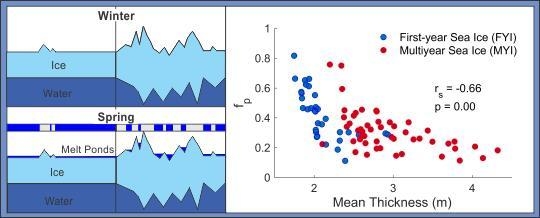
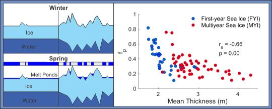
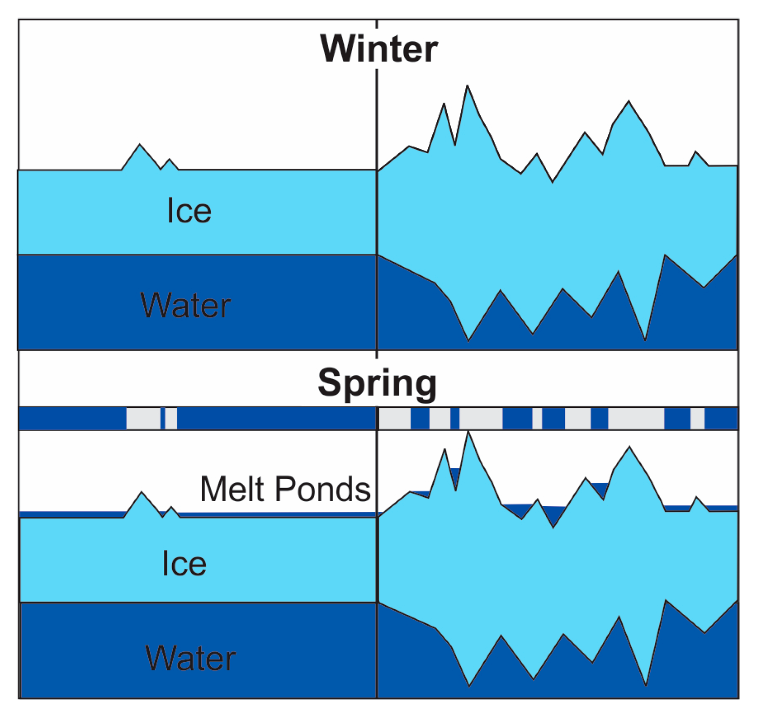
It has been shown that spring melt pond fraction can be used to accurately forecast September minimum sea ice extent. This result is explained by the following positive feedback mechanism: increase in melt pond fraction reduces the surface albedo; a lower albedo leads to more melting; increased melting leads to a further increase in melt pond fraction [10]. In addition, it is generally understood that sea ice that is thin and has low surface roughness in the winter will have a high spring fp and ice that has been dynamically thickened and roughened will have a low fp [11] (Figure 1). This study aims to establish a link between winter conditions and spring fp in order to evaluate to what extent the ice cover is pre-conditioned for spring melt. The goal of this paper is to quantify relationships between winter sea ice thickness, roughness, and spring fp for an area comprising a mixture of landfast FYI and MYI in the Canadian Arctic Archipelago (CAA). Explicitly we first investigate the macro-scale relationships between winter sea ice thickness and roughness, and spring fp; followed by an investigation of how these relationships differ between FYI and MYI.
2. Materials and Methods
2.1. Study Area
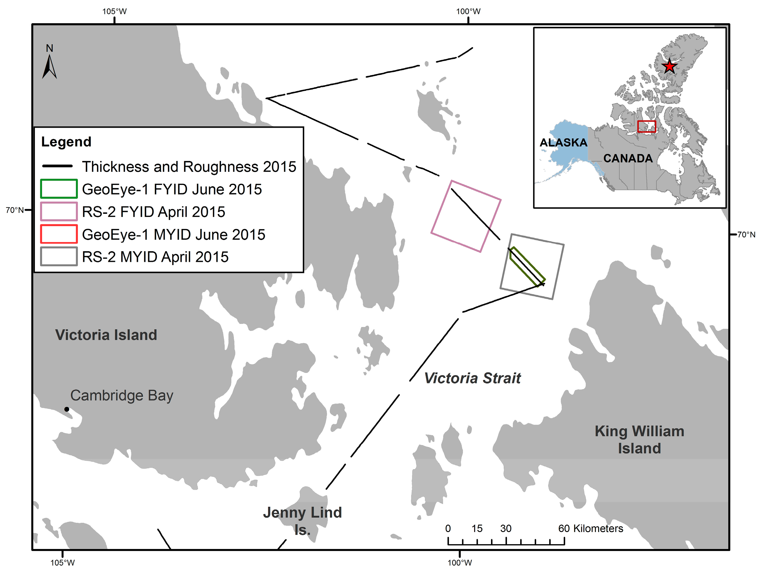
Airborne winter snow plus sea ice thickness and surface roughness transects and satellite GeoEye-1 optical and RADARSAT-2 (RS-2) SAR images were collected in Victoria Strait region of the CAA during April and June 2015 (Table 1; Figure 2). Victoria Strait is part of the Northwest Passage in the CAA, which typically contains a mixture of FYI and MYI. The sea ice in the CAA is not strongly affected by wind driven movement because the ice is landfast for six to eight months of the year [21]. Furthermore, wind driven movement of sea ice is restricted by the narrow channels that dominate the CAA [22]. During the melt season, MYI drifts into and subsequently through the CAA from the central Arctic during late summer and early fall and becomes locked in place by FYI that forms in the fall and early winter [23]. This makes for an ideal study area for understanding the evolution of sea ice from winter to summer conditions, without the need for tracking mobile ice.
The FYI-dominated (FYID) zone (Figure 3, left) is characterized by thinner and smoother ice compared to the MYI-dominated (MYID) ice zone (Figure 3, right). The majority of the ice within the FYID zone is under 2.5 m thick, compared to the MYID zone, which is dominated by ice thicker than 2.5 m. Similarly, the FYID zone is smoother than the MYID, with areas of thicker ice corresponding to rougher ice in both areas.
2.2. Data and Pre-Processing
Airborne winter snow plus sea ice thickness and surface roughness data were acquired during a late winter survey flown on 19 April 2015 [24] (Table 1; Figure 2). The survey was conducted in late April in order to capture the late winter conditions indicative of maximum sea ice thickness and reduce the amount of surface variability associated with atmospheric processes such as surface erosion and wind-driven snow redistribution [24]. The snow plus ice thickness was obtained using an airborne electromagnetic (EM) thickness sounding instrument [25]. The EM instrument induces an EM-field in the conductive sea water under the resistive sea ice from which the height of the instrument above the ice/water interface can be derived [25]. A single-beam laser altimeter included in the EM instrument measures the height of the system above the top of the snow cover. The difference between those two measurements is the total thickness, i.e., snow plus ice thickness. It is not possible to distinguish between snow and ice thicknesses because both snow and ice are very resistive. Therefore snow plus ice thickness is hereafter referred to as ice thickness [24,25]. This strongly oversamples the ice because EM measurements have a footprint of approximately 3 to 4 times the instrument height above the ice. With typical instrument heights below 30 m this corresponds to a footprint of up to 120 m. The sampling rate was 10 scans per minute therefore thickness observations were obtained approximately every 6 m.
A Riegel Laser Measurements Systems (Riegel LMS) Q120 near infrared laser scanner was used to collect 2D swaths of relative surface elevation measurements. Each scan line was then approximated with a flat surface hyperbolic equation and surface roughness was calculated from each scan line as the standard deviation of the difference between measured and fitted surfaces [26]. The obtained surface roughness therefore corresponds to root-mean-square (RMS roughness along the approximately 105 m wide swath perpendicular to the flight direction. The scanning rate was 50 lines per second, resulting in surface roughness measurements of approximately 1.2 m apart.
Two high-resolution panchromatic (0.5 m) and multispectral (2.0 m) optical image bundles of spring melt pond covered FYID (23 × 5.3 km) and MYID (26.5 × 5.2 km) zones were acquired between 23 and 25 June, 2015 from the GeoEye-1 sensor (Figure 3). In order to combine the high spatial resolution of the panchromatic imagery and high spectral resolution of the multispectral imagery, image pairs were fused together using a Gram-Schmidt (GS) pan-sharpening algorithm. The GS algorithm was chosen because it preserves the spectral and spatial integrity of the original imagery [27]. Pan-sharpened images were classified using a Maximum Likelihood (ML) supervised classification algorithm to yield a binary output: ice (0) and pond (1). Classification accuracies were calculated using confusion matrices built from a range of 50 to 96 samples representing homogeneous ice and melt pond areas. This approach yielded overall accuracies of >99% with kappa coefficients of >0.9. The classified images allowed for calculation of fp for regions of interest in the scene using the following equation:
where represent the sum of pond pixels and Total Count is the total number of pixels within the region of interest such as an image object or entire scenes. A flow chart depicting the pre-processing chain and subsequent analyses is given in Figure 4.
2.3. Object Based, Hybrid and Grid-Cell Image Analysis
Two winter RS-2 Fine Quad-polarization (FQ) format SAR images of the FYID and MYID zones were acquired between 23 and 25 April 2015 were used for segmentation into image objects (Figure 4, left). The multiresolution segmentation approach implemented in the OBIA-driven software eCognition (Trimble) was used for segmentation. This approach has been proven to be effective for image segmentation related to cut block and tree crown delineation, classification of agricultural landscapes, ship detection and sea ice studies [28,29,30,31,32]. Using a bottom up region merging approach, objects are generated based on user defined spatial and spectral heterogeneity criteria, as well as a scale criterion used to control object size. Spatial heterogeneity is related to shape of the object, whereas spectral heterogeneity is variance of data within the object [33]. Emphasis was placed on deriving a segmentation that yielded image objects displaying within-object homogeneity and between-object heterogeneity and representing unique ice floes. To account for some uncertainty in boundary delineation, multiple object sets were created by varying the scale parameter in the segmentation algorithm. For the MYID zone, object features at the fine, medium and coarse scales were delineated. For the FYID zone, object features at fine and medium scales were created. Due to a lack of heterogeneity in the FYID zone, objects were not created at a coarse spatial scale. This was necessary for calculating global FYI and MYI statistics regardless of whether objects originated in FYID or MYID zones.
Three different approaches for aggregating and deriving statistics of ice thickness, roughness, and fp data were used (Figure 5). The first approach, object, used original image objects that intersected the airborne track. The second approach, hybrid, used original image segmented objects intersecting the flight line but also accounted for the across-track footprint of the airborne laser scanner (~105 m). The hybrid objects were generated by reducing the extent of the original objects to an across-track width of 120 m. The two approaches yielded a total of 61, 50 and 41 objects representative of MYI floes from fine, medium, and coarse scale segmentation, respectively. Conversely, fine and medium scale segmentation of FYI yielded 53 and 33 objects, respectively. Finally, the third approach involved the overlay of grid-cells centered on the flight line. Two sets of grid-cell features were created for both FYID and MYID zones, one with across-track widths of 120 m and along-track lengths of 120 m, and one with across-track widths of 120 m and along-track lengths of 240 m. This yielded a total of 210 (120 × 120 m) and 103 (120 × 240 m) grid-cells features for the FYI zone, and 109 (120 × 120 m) and 56 (120 × 240 m) grid-cell features for the MYI zone. In order to avoid loss of data, grid-cells that were dominated by FYI and located in the MYID zone were analyzed as FYI, and vice versa.
The average areas (and ranges) of FYI object segments at fine and medium spatial scales were 0.50 km2 (0.03–1.42 km2) and 1.35 km2 (0.25–5.08 km2), respectively, whereas the average areas of MYI object segments at fine, medium and coarse scales were 0.29 km2 (0.03–0.92 km2), 0.44 km2 (0.04–1.19 km2) and 0.63 km2 (0.04–1.97 km2), respectively. Hybrid objects were generated by decreasing across-track extent of objects to 120 m. Thus, average areas of hybrid objects were smaller than the object segments, with mean FYI segment areas of 0.05 km2 (0.002–0.16 km2) and 0.08 km2 (0.01–0.31 km2) for fine and medium spatial scales, respectively. Average areas of MYI hybrid objects were 0.03 km2 (0.003–0.10 km2) at the fine scale, 0.04 km2 (0.01–0.14 km2) at the medium and 0.04 km2 (0.01–0.14 km2) at the coarse spatial scales. The areas of individual grid-cells remained consistent at 0.014 km2 and 0.017 km2 for 120 m and 240 m kernels, respectively.
The three data aggregation approaches at varying spatial scales enabled the examination of relationships between winter sea ice thickness, roughness and fp, as well as the role of scale and aggregation approaches on those relationships. First, a 2000 point moving average was applied on the roughness data in an attempt to minimize the effects of snow roughness on the surface roughness measurements. 4000 points outside of both the FYID and MYID zones were used for the calculation of the moving average. Probability distributions of winter sea ice thickness, surface roughness, smoothed roughness, and spring fp were plotted for FYI and MYI, with fp values obtained using hybrid aggregation at the medium scale. For quantifying relationships, aggregated roughness and thickness metrics (minimum, maximum, mean, median and standard deviation (SD)) were each compared to fp within each aggregation feature. Spearman correlation coefficients were collected to assess the strength of relationships between thickness and roughness, thickness and fp, and roughness and fp for FYI and MYI. Spearman correlation was chosen because it is a non-parametric measure of association between two variables. An ordinary least squares (OLS) regression analysis was performed with roughness and thickness as independent variables, and fp as the dependent variable. For the OLS, a non-linear rational function was fitted to the thickness and fp data because it is more representative of the expected variation in fp. It is expected that fp will behave asymptotically when approaching values of 0 and 1, which will not be captured by a linear function. A rational function is beneficial for modelling physical processes because it allows for better fit of data with a relatively complex distribution, while retaining computational and structural simplicity associated with linear regression. A linear function was fitted to the roughness and fp data because of its representative fit and computational simplicity.
3. Results
3.1. Victoria Strait Thickness, Roughness and fp Distributions in 2015
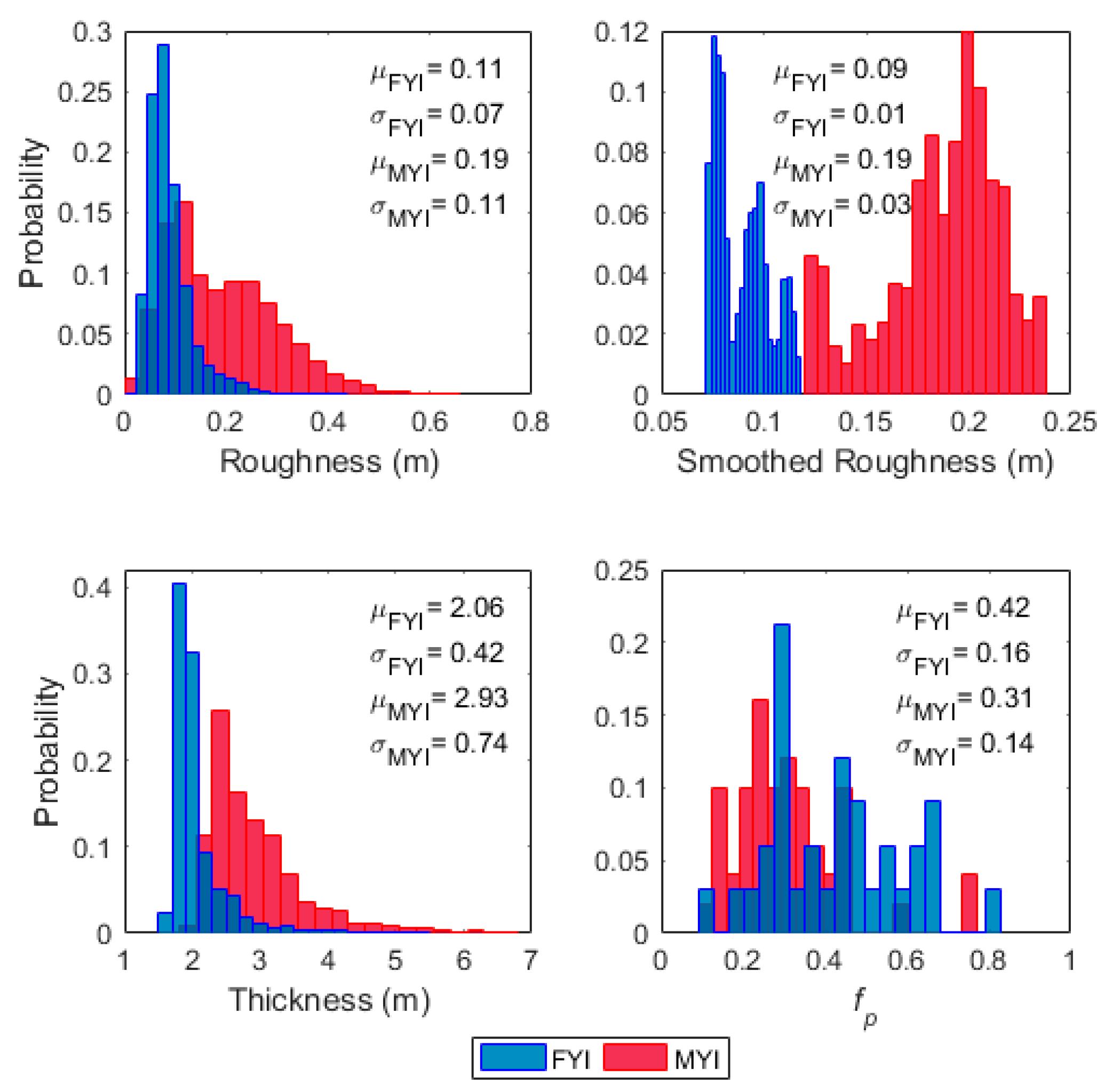
FYI was characterized by lower winter thickness and surface roughness, and higher spring fp compared to MYI (Figure 6). FYI winter sea ice thickness ranged between 1.6 and 5.5 m, with mean and median thicknesses of 2.1 and 1.9 m, respectively. Conversely, MYI thickness ranged between 1.8 and 6.7 m, with mean and median values of 2.9 and 2.7 m, respectively. The surface roughness on FYI ranged between 0.02 and 0.81 m, with mean and median roughness values of 0.11 and 0.09 m, respectively. Conversely, MYI surface roughness measurements ranged between 0.02 and 0.65 m, with mean and median values of 0.19 and 0.17 m, respectively. Smoothed surface roughness (2000 point moving average) shows increased separability between FYI and MYI. FYI smoothed surface roughness values ranged between 0.08 m and 0.12 m with mean and median values of 0.09 m, whereas MYI smoothed surface roughness values between 0.12 m and 0.24 m were observed with mean and median values of 0.19 m. Finally, spring fp values were between 0.19 and 0.71 for FYI, and 0.12 and 0.77 for MYI with mean values of 0.43 and 0.29 for FYI and MYI, respectively.
3.2. Relationship between Thickness and fp
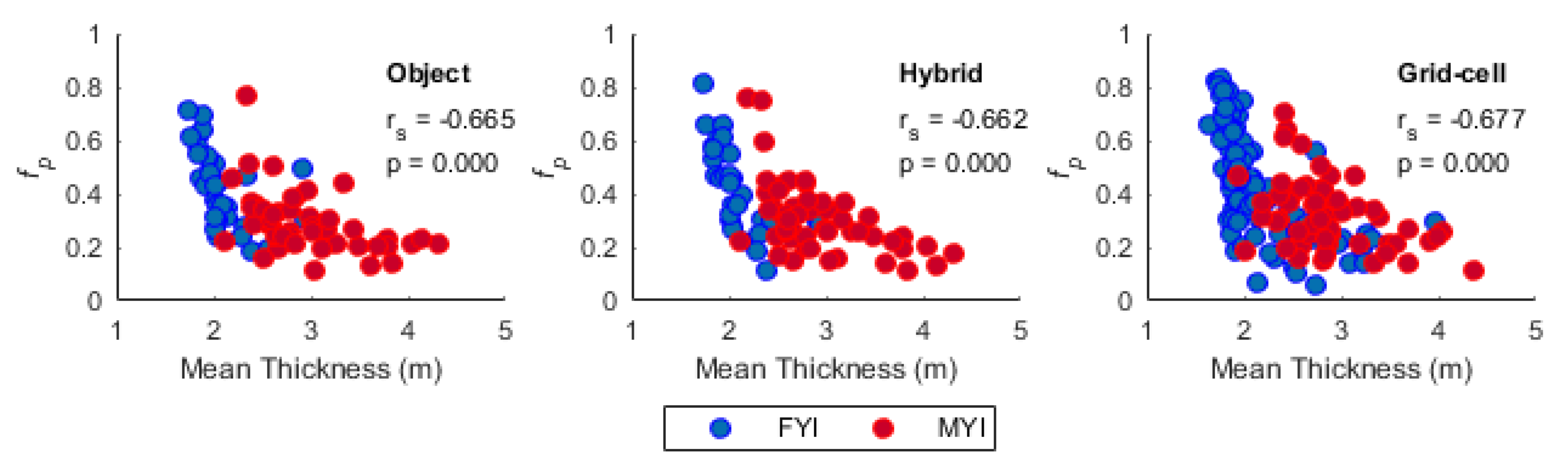
FYI thickness exhibited statistically significant negative correlations (p < 0.05) with fp for all analyzed scales and aggregation approaches (object, hybrid, grid-cell) (Table 2; Figure 7). Whereas all metrics of MYI thickness showed statistically significant negative correlations at fine scales (object and hybrid) and 120 m grid-cells. Overall, the hybrid-based aggregation approach yielded the strongest statistically significant negative correlations between winter sea ice thickness and fp for both FYI and MYI, particularly for mean thickness and fp. Furthermore, the distribution of mean thickness and corresponding fp values showed less variability using the hybrid-based approach, compared to the object and grid-cell-based approaches at the medium/240 m spatial scales (Figure 7). This affirms that mean sea ice thickness is strongly related to fp, particularly within the range of the EM-bird footprint, which is approximately 120 m, depending on the height of the instrument above the sea ice surface [25]. The dependence of fp on mean thickness can be explained by the presence or absence of deformation features. Thin FYI that has not undergone dynamic forcing is very level/smooth and will experience widespread flooding and higher fp. Conversely, FYI that has undergone ridging will constrain melt water into deeper surface depressions.
The rational function OLS model used to determine the ability of winter FYI and MYI thickness to explain the variability in spring fp is shown in Figure 8. Thickness and fp data aggregated at the medium scale using the hybrid aggregation approach were used as inputs for the OLS model because they showed the strongest associations for FYI and MYI in the correlation analysis and exhibited lower variance than the object and grid-cell approaches. The model indicates that 47% of the variation in fp can be explained using mean thickness according to Equation (2).
3.3. Relationship between Roughness and fp
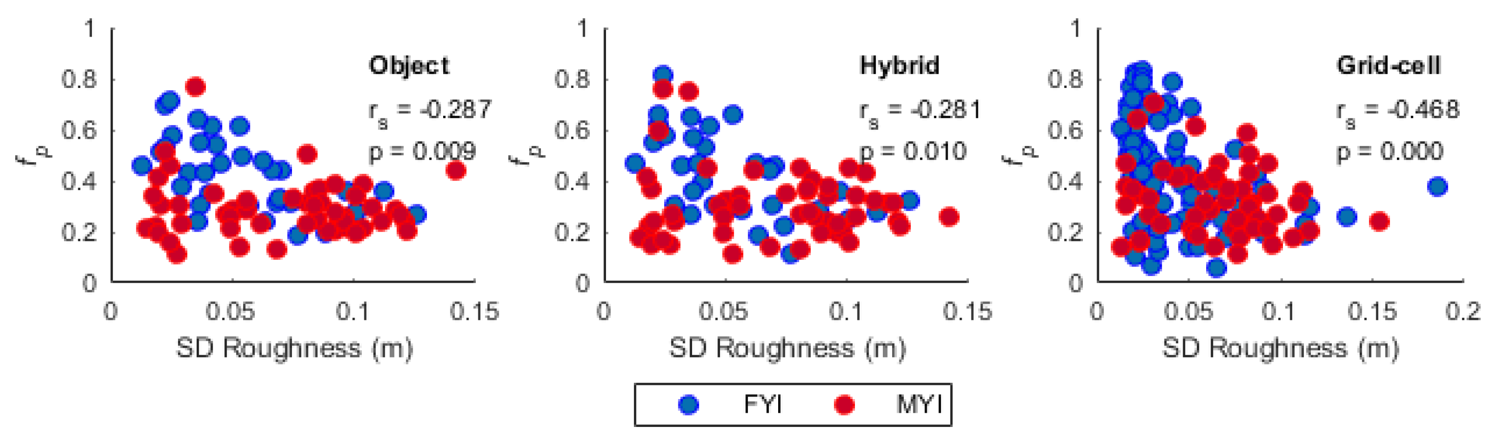
Surface roughness exhibited moderate negative correlations with fp for FYI using all three aggregation approaches and at all analyzed spatial scales. Object and hybrid aggregation approaches produced stronger associations compared to the grid-cell method (Table 3; Figure 9). For FYI, the standard deviation of roughness showed the strongest negative association with fp, particularly at the medium scale. This shows that variability in surface roughness is related to melt pond distribution at the analyzed scale, i.e., greater surface roughness variability leads to lower fp. A high variability in surface roughness on FYI can be due to the presence of compression ridges and snow sastrugi in areas of otherwise smooth ice. Conversely, low variability in surface roughness on FYI is attributed to smooth, thermodynamically grown ice, which lacks deformation features and easily floods when melt ponds form. Interestingly, metrics of surface roughness did not show any statistically significant correlations with fp for MYI, except for a weak positive relationship between minimum roughness and fp at the fine spatial scale using object-based aggregation. It is important to note that MYI exhibits greater spatial variability in surface roughness than FYI (Figure 3). Quantifying surface roughness on MYI, compared to relatively smooth FYI, and relating it to fp poses a unique challenge due to the lack of level ice in MYI-dominated areas. Level ice is necessary for the calculation of the local level-ice surface used in the calculation of surface roughness. The absence of level ice will lead to an overestimation of the local level-ice surface, which will lead to an overall overestimation of surface roughness from the 2D laser scanner [26]. Furthermore, areas of uniformly weathered MYI will have a low winter surface roughness, corresponding to a low spring fp, whereas an area composed of both rough MYI and smooth ice, such as a re-frozen melt pond from a previous melt season, will be characterized by a high standard deviation of relative surface height (i.e., high winter roughness), which will correspond to a high spring fp due to flooding on areas of smooth ice. Finally, the snow pack will likely be deeper on MYI than FYI because MYI begins accumulating snow earlier than FYI and surface depression in MYI act as catchments for wind-blown snow.
The linear OLS model used to assess the explanatory power of surface roughness for variations in spring fp is shown in Figure 10. It was found that the SD of winter surface roughness explained 11% of the variability in spring fp. However, surface roughness was a statistically significant dependent variable, which suggests that it contains explanatory power for variability in fp.
3.4. Relationship between Smoothed Surface Roughness and fp
Snow on sea ice will likely affect surface roughness estimates by masking the signal associated with sea ice surface roughness with snow redistribution features such as dunes and snow roughness features such as sastrugi, which are wavelike features that occur on the surface of hard snow that have been redistributed by wind action. A 2000 point (~2400 m) moving average was used to effectively average out footprint-scale variability likely associated with snow roughness and snow redistribution features. A significantly stronger correlation was found between metrics of FYI roughness and fp, with highest associations observed at the medium spatial scale (Figure 11; Table 4). Moderate statistically significant correlations can be observed between metrics of MYI roughness and fp, particularly using the object aggregation approach at the fine spatial scale. It is important to note that smoothing the surface roughness data allows for an increased separability between FYI and MYI (Figure 6, top right) compared to unsmoothed data (Figure 6, top left). This result suggests that small-scale uncertainties associated with surface roughness measurements are removed when investigating these relationships at regional scales appropriate for studies utilizing satellite observations. However, this approach warrants caution as it introduces increased spatial dependency or spatial autocorrelation between individual measurements.
3.5. Relationship between Thickness and Roughness
Areas of thick ice are coincident with areas of high surface roughness, particularly for FYID as illustrated in Figure 3. Quantitatively, maximum roughness and maximum thickness show a significant positive association for both FYI and MYI using the object aggregation approach (Table 5; Figure 12). FYI shows a stronger relationship (rs = 0.65) than MYI (rs = 0.54) at medium spatial scale. The grid-cell-based aggregation approach yields statistically significant correlations between all metrics of roughness and thickness for FYI, and no significant associations for MYI. The variance in FYI and MYI observations is lower using object-based aggregation, compared to 240 m grid-cells (Figure 12). Finally, it can be seen that variance begins to increase for ice with thickness of greater than approximately 3.75 m. It is expected that thicker ice has undergone more dynamic thickening when compared to thin ice, which would increase both the thickness and the surface roughness. The EM instrument measures the bottom roughness of the ice, which would also be roughened during ridging and rafting. This would lead to an increase in the strength of association between ice thickness and surface roughness.
4. Discussion
Previous studies have shown that FYI is characterized by a higher spring fp than MYI [7,11,13,34,35]. Our findings support these observations, with FYI exhibiting on average higher spring fp of 0.43 compared to 0.29 for MYI. However, we show that certain regions of MYI become flooded, with spring fp reaching up to 0.77. Winter sea ice thickness and surface roughness values and probability distributions are consistent with previous studies, showing FYI being thinner and smoother compared to MYI. Numerical models indicate that pre-melt surface roughness is strongly related to fp, with fp increasing more rapidly on a smoother ice than rougher ice [36]. Our results show that surface roughness is related to fp for FYI, but we do not find a similar association for MYI. Previous work has suggested that thin and smooth ice would be favorable for high fp during the melt season, and rough/thick ice would limit melt pond expansion and result in low fp; however these relationships have not been quantified to date [11,37]. For logistical reasons the majority of previous melt pond evolution studies have been conducted on landfast FYI and drifting MYI. Our fp observations show agreement with other landfast FYI studies and drifting FYI and MYI studies. Since our analyses are concerned with one snapshot of melt fraction, and not melt pond evolution through time, it is not necessary to account for ice mobility. However, when considering melt pond evolution, it is important to note that thermodynamic and dynamic processes of landfast ice differ from those of drifting ice. Landfast sea ice forms in areas of shallow bathymetry and is influenced by tides and nearshore currents [38]. Furthermore, it exhibits a fixed orientation with the respect to the sun and is influenced by dust and warm air from the nearby land [39].
Considering the role of different aggregation approaches for quantifying relationships, the benefit of OBIA is that it is rooted in real world features such as ice floes, thus providing physically meaningful extents for data aggregation and contextual information for the analyst. The hybrid approach aims to compromise between the extents of real world features and the footprint of the sensor, in cases where objects are being used to aggregate multi-sensor data. In this study, the extents of the objects were often much larger than the footprint of the thickness and roughness sensors, which means that the corresponding thickness and roughness measurements may not have been representative of certain regions of the object (Figure 5). The hybrid object approach yielded stronger associations between thickness and fp for FYI and similar to slightly stronger relationships for MYI (Table 2). The stronger relationships between FYI thickness and fp can be explained by spatial homogeneity of FYI ice floes in terms of thickness, roughness and the SAR backscatter used to delineate objects. Compared to MYI, FYI has a lower surface roughness, which allows it to have a low backscatter across large areas. By reducing the width of the object-based features into hybrid objects, analyses become more representative of the areas associated with the thickness and roughness measurements while retaining the across-track boundaries of individual ice floes.
We have been able to show that winter sea ice thickness and surface roughness are related to spring fp on landfast sea ice in the CAA; however, it is possible that sensor limitations impacted the results. Laser altimeters do not penetrate through the snow cover to the snow/ice interface, therefore the sea ice thickness measurements obtained using the EM-bird are in actuality snow plus ice measurements. It is suggested that the accuracy of EM measurements over level ice is approximately ±0.15 m, whereas thickness of thick MYI ridges can be underestimated by as much as 24%. Areas of thick ice, such as ridges in an otherwise smooth FYI zone can be underestimated if they are proximal to areas of thin ice and occur with the footprint of the EM sensor. Unfortunately, it was not possible to obtain co-located in situ snow depth observations in our study area and due to the uncertainties associated with snow depth estimates in complex ice environments Operation IceBridge (OiB) and CryoVex data were not included in the analyses [40]. We were able to obtain in situ snow depth measurements, which were collected using a MagnaProbe near Eureka in the CAA between 8 and 15 April 2016 (Figure 2). 1792 and 1810 snow measurements were collected on FYI and MYI, respectively, with transects covering areas of approximately 0.4 km2 each (~10 m spacing).
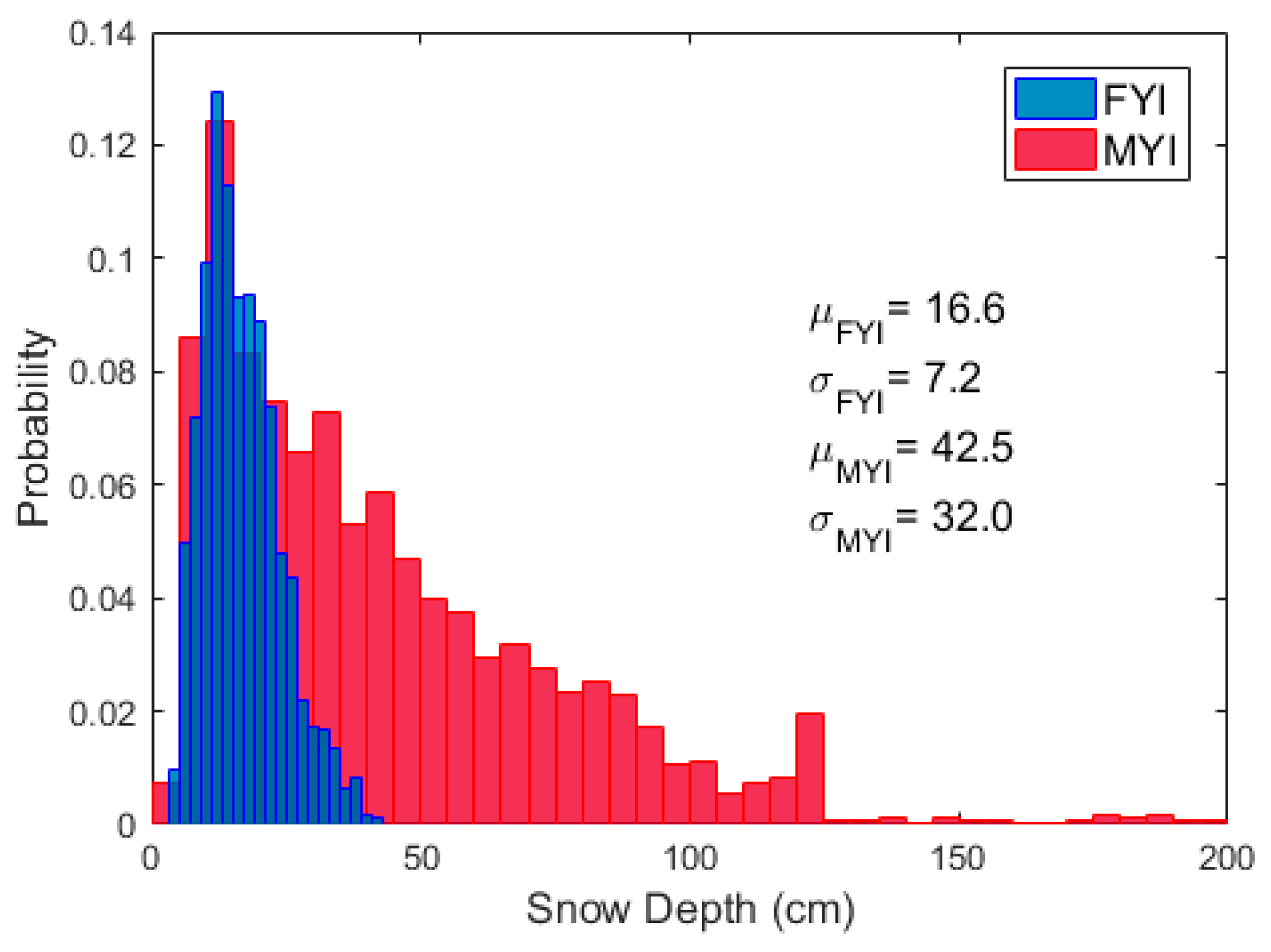
Figure 13 shows that the mean snow depth on FYI is 16.6 cm compared to 42.5 cm on MYI. The variability in snow depth is also greater for MYI, with depths of up to 200 cm. In 2016, total October to May snowfall at an Environment Canada station in Cambridge Bay was approximately 45 cm compared to 65 cm at an Environment Canada station in Eureka. October to May in situ mean snow depths on landfast FYI measured 8.4 ± 4.2 cm (Cambridge Bay) and 17.6 ± 5.8 cm (Eureka) between 1960 and 2014 [41]. The nearest snow depth and weather station data available indicate that Victoria Strait will have less sea ice snow accumulation than Eureka. Further work or co-located snow depth and EM sea ice thickness measurements would be required to more fully assess the effect of snow depth on relationships with fp.
The 2D laser scanner instrument operates in the near infrared part of the electromagnetic spectrum, which means that it does not penetrate through the snow cover and thus measures variations in snow topography. This could potentially lead to underestimation of surface roughness because the snow cover may have a dampening effect on the sea ice surface, particularly due to accumulation of snow in rough areas by wind redistribution. Snow sastrugi may also introduce erroneous surface roughness values that are not associated with the sea ice topography. Quantifying surface roughness in the natural environment remains a challenge, with the most widely used approach being the standard deviation of relative surface elevation; however other statistical parameters such as skewness and kurtosis have been proposed [42]. Furthermore, roughness measurements are highly scale-dependent and large-scale variations in topography may introduce uniform and along flight line errors. Finally, it is often assumed that distribution of sea ice features such as ridges and leads is random. However, this assumption is often not valid because dominant orientations of features result from prevailing ocean and atmospheric currents. Thus, it is possible to under or over represent the distribution of extreme features, depending on the choice of flight direction [25].
Thermodynamic and dynamic processes are responsible for changes in sea ice thickness with FYI increasing above modal thickness as a result of ridging. Thus, surface roughness and ice thickness are expected to be closely related, particularly for thicker, more deformed FYI. This is supported by comparing the spatial distribution of high thickness and roughness values for FYI in the study area (Figure 3). Areas of high surface roughness (0.33–0.44 m) overlap with areas of thicker ice (2.7–3.1 m), as well as with areas of higher backscatter. A similar relationship can be seen for MYI. Quantitatively, we have shown that maximum thickness and maximum roughness have a stronger association for FYI (rs = 0.65) than MYI (rs = 0.54). With MYI being ice that survived one or more melt season, its surface roughness will be affected by melt, particularly by the presence of refrozen melt ponds from previous melt seasons. An area that includes a melt pond from a previous melt season and heavily deformed patch of ice may be associated with high surface roughness measurement. However, this high roughness value may correspond to a high fp due to the presence of a relatively smooth patch of ice, which was previously occupied by a melt pond.
5. Conclusions
The primary goal of this study was to quantitatively link winter sea ice thickness and surface roughness to spring fp in order to better understand how the ice evolves from winter to spring thermodynamic states and inform parameterizations of fp in climate models. This was achieved by evaluating the utility of object-based image analysis, hybrid-object analysis, which takes into account the footprints of the thickness and roughness sensors, as well as the traditional grid-cell data aggregation approaches. It was found that winter sea ice thickness has a strong association with fp for FYI (rs = −0.85) and MYI (rs = −0.64) using hybrid aggregation approach, as well as the object approach for FYI (rs = −0.75) and MYI (rs = −0.60). Weaker relationships were observed for MYI using the grid-cell approach (rs = −0.47); however a similar relationship was detected for FYI (rs = −0.75). This shows that winter sea ice thickness is related to spring fp with thicker ice characterized by lower spring fp and thin ice exhibiting a higher fp during the melt season. These results provide a quantitative link between the two geophysical parameters and have important implications for understanding spring fp evolution on Arctic sea ice. The stronger relationships observed using hybrid aggregation indicate that accounting for ice morphology and sensor footprints allows for more representative comparison between multisource datasets. A non-linear rational function OLS model shows that 47% of variability in combined FYI and MYI spring fp can be explained by mean winter sea ice thickness using the hybrid-based aggregation approach indicating a potential for spring fp prediction using winter sea ice thickness.
FYI spring fp is related to winter surface roughness, with a stronger relationship observed using the hybrid-based aggregation approach at the medium scale (rs = −0.63). However, MYI fp is not significantly correlated with surface roughness. Surface roughness can be defined for scales ranging from meters to kilometers, with footprint-scale uncertainties such as snow roughness and errors associated with sensor position during airborne measurement acquisition (yaw and pitch angles, and slant range distortion) exhibiting a stronger effect on the measurements than at larger spatial scales [26,40]. In order to minimize the influence of measurement uncertainty on surface roughness measurements we performed a moving average on the surface roughness data (~2400 m) and found stronger correlations between surface roughness and fp for both FYI (rs = −0.84) and MYI (rs = −0.34). We propose that further work is conducted on assessing the effects of snow depth and snow redistribution features on sea ice surface roughness estimates.
Winter sea ice thickness and surface roughness are strongly correlated for FYI (rs = 0.65) and MYI (rs = 0.54) using the object aggregation approach. These relationships are lower in strength for FYI (rs = 0.53) and are not present for MYI using the grid-cell data aggregation approach. This further supports the use of object-based aggregation for spatial statistical analyses.
This study draws quantitative linkages between winter sea ice (snow plus ice) thickness and spring fp at the macro scale, which can contribute to a body of work improving parametrizations of spring fp in climate models. Further work includes contributing evaluations of the potential of winter sea ice thickness, in addition to sea ice roughness, as well as radar backscatter signatures to predict spring fp using satellite sensors such as CryoSat-2, Sentinel-1 and others. It is important to be able to expand the analyses to larger spatial and temporal scales, which are necessary for initializing and validating regional climate models.
Acknowledgments
The research was conducted as part of the interdisciplinary Ice Covered Ecosystem-CAMbridge Bay Process Studies (ICE-CAMPS) project. Funding was provided by Marine Environmental Observation Prediction and Response Network (MEOPAR) and the National Sciences and Engineering Research Council of Canada (NSERC)—Discovery Grants Program. Additional support was provided by the Northern Scientific Training Program (NSTP).
Author Contributions
Sasha Nasonova prepared the datasets, conducted the quantitative analysis and drafted the manuscript. Randy Scharien conceived the study, processed and segmented the RADARSAT-2 imagery, provided expert interpretation of the data and results, and contributed extensive feedback on the manuscript. Christian Haas provided thickness and roughness data for the analysis as well expert interpretation and support. Stephen Howell conceived the study and provided the RADARSAT-2 and GeoEye-1 datasets.
Conflicts of Interest
The authors declare no conflict of interest.
References
- Rigor, I.G.; Wallace, J.M. Variations in the age of Arctic sea-ice and summer sea-ice extent. Geophys. Res. Lett. 2004, 31, 2–5. [Google Scholar] [CrossRef]
- Kwok, R.; Cunningham, G.F.; Wensnahan, M.; Rigor, I.; Zwally, H.J.; Yi, D. Thinning and volume loss of the Arctic Ocean sea ice cover: 2003–2008. J. Geophys. Res. 2009, 114. [Google Scholar] [CrossRef]
- Meier, W. Actic sea ice in tranformation: A review of recent observed changes and impacts on biology. Rev. Geophys. 2015, 53, 1–33. [Google Scholar] [CrossRef]
- Swart, N.C.; Fyfe, J.C.; Hawkins, E.; Kay, J.E.; Jahn, A. Influence of internal variability on Arctic sea-ice trends. Nat. Clim. Chang. 2015, 5, 86–89. [Google Scholar] [CrossRef]
- Hanesiak, J.M.; Barber, D.G.; De Abreu, R.A.; Yackel, J.J. Local and regional albedo observations of arctic first-year sea ice during melt ponding. J. Geophys. Res. 2001, 106, 1005–1016. [Google Scholar] [CrossRef]
- Perovich, D.K.; Polashenski, C. Albedo evolution of seasonal Arctic sea ice. Geophys. Res. Lett. 2012, 39, 1–6. [Google Scholar] [CrossRef]
- Perovich, D.K.; Grenfell, T.C.; Light, B.; Hobbs, P.V. Seasonal evolution of the albedo of multiyear Arctic sea ice. J. Geophys. Res. 2002, 107. [Google Scholar] [CrossRef]
- Arrigo, K.R.; Perovich, D.K.; Pickart, R.S.; Brown, Z.W.; van Dijken, G.L.; Lowry, K.E.; Mills, M.M.; Palmer, M.A.; Balch, W.M.; Bahr, F.; et al. Massive Phytoplankton Blooms Under Arctic Sea Ice. Science 2012, 336, 1408. [Google Scholar] [CrossRef] [PubMed]
- Pućko, M.; Stern, G.A.; Macdonald, R.W.; Jantunen, L.M.; Bidleman, T.F.; Wong, F.; Barber, D.G.; Rysgaard, S. The delivery of organic contaminants to the Arctic food web: Why sea ice matters. Sci. Total Environ. 2015, 506–507, 444–452. [Google Scholar] [CrossRef] [PubMed]
- Schröder, D.; Feltham, D.L.; Flocco, D.; Tsamados, M. September Arctic sea-ice minimum predicted by spring melt-pond fraction. Nat. Clim. Chang. 2014, 4, 353–357. [Google Scholar] [CrossRef]
- Eicken, H.; Grenfell, T.C.; Perovich, D.K.; Richter-Menge, J.A.; Frey, K. Hydraulic controls of summer Arctic pack ice albedo. J. Geophys. Res. Oceans 2004, 109, 1–13. [Google Scholar] [CrossRef]
- Eicken, H. Tracer studies of pathways and rates of meltwater transport through Arctic summer sea ice. J. Geophys. Res. 2002, 107, 1–20. [Google Scholar] [CrossRef]
- Polashenski, C.; Perovich, D.; Courville, Z. The mechanisms of sea ice melt pond formation and evolution. J. Geophys. Res. 2012, 117, 1–23. [Google Scholar] [CrossRef]
- Rösel, A.; Kaleschke, L.; Birnbaum, G. Melt ponds on Arctic sea ice determined from MODIS satellite data using an artificial neural network. Cryosphere 2012, 6, 431–446. [Google Scholar] [CrossRef] [Green Version]
- Scharien, R.K.; Hochheim, K.; Landy, J.; Barber, D.G. First-year sea ice melt pond fraction estimation from dual-polarisation C-band SAR – Part 2: Scaling in situ to Radarsat-2. Cryosphere 2014, 8, 2163–2176. [Google Scholar] [CrossRef]
- Han, H.; Im, J.; Kim, M.; Sim, S.; Kim, J.; Kim, D.J.; Kang, S.H. Retrieval of melt ponds on arctic multiyear sea ice in summer from TerraSAR-X dual-polarization data using machine learning approaches: A case study in the Chukchi Sea with mid-incidence angle data. Remote Sens. 2016, 8, 57. [Google Scholar] [CrossRef]
- Kettig, R.L.; Landgrebe, D.A. Classification of Multispectral Image Data by Extraction and Classification of Homogeneous Objects Classification of Multispectral Image Data by Extraction and Classification of Homogeneous Objects. IEEE Trans. Geosci. Electron. 1976, 14, 19–26. [Google Scholar] [CrossRef]
- Blaschke, T. Object based image analysis for remote sensing. ISPRS J. Photogramm. Remote Sens. 2010, 65, 2–16. [Google Scholar] [CrossRef]
- Hay, G.; Marceau, D.; Dube, P.; Bouchard, A. A Multiscale Framework for Landscape Analysis: Object-specific analysis and upscaling. Landscape 2001, 16, 471–490. [Google Scholar]
- Mazur, A.K.; Wåhlin, A.K.; Krężel, A. An object-based SAR image iceberg detection algorithm applied to the Amundsen Sea. Remote Sens. Environ. 2017, 189, 67–83. [Google Scholar] [CrossRef]
- Canadian Ice Service. Sea Ice Climatic Atlas: Northern Canadian Water 1981-2010; Environment Canada: Ottawa, ON, Canada, 2007.
- Melling, H. Sea ice of the northern Canadian Arctic Archipelago. J. Geophys. Res. Ocean. 2002, 107. [Google Scholar] [CrossRef]
- Howell, S.E.L.; Wohlleben, T.; Dabboor, M.; Derksen, C.; Komarov, A.; Pizzolato, L. Recent changes in the exchange of sea ice between the Arctic Ocean and the Canadian Arctic Archipelago. J. Geophys. Res. Oceans 2013, 118, 3595–3607. [Google Scholar] [CrossRef]
- Haas, C.; Howell, S.E.L. Ice thickness in the Northwest Passage. Geophys. Res. Lett. 2015, 1–8. [Google Scholar] [CrossRef]
- Haas, C.; Lobach, J.; Hendricks, S.; Rabenstein, L.; Pfaf, A. Helicopter-borne measurements of sea ice thickness, using a small and lightweight, digital EM system. J. Appl. Geophys. 2009, 67, 234–241. [Google Scholar] [CrossRef] [Green Version]
- Beckers, J.F.; Renner, A.H.H.; Spreen, G.; Gerland, S.; Haas, C. Sea-ice surface roughness estimates from airborne laser scanner and laser altimeter observations in Fram Strait and north of Svalbard. Ann. Glaciol. 2015, 56, 235–244. [Google Scholar] [CrossRef]
- Sarp, G. Spectral and spatial quality analysis of pan-sharpening algorithms: A case study in Istanbul. Eur. J. Remote Sens. 2014, 47, 19–28. [Google Scholar] [CrossRef]
- Flanders, D.; Hall-Beyer, M.; Pereverzoff, J. Preliminary evaluation of eCognition object-based software for cut block delineation and feature extraction. Can. J. Remote Sens. 2003, 29, 441–452. [Google Scholar] [CrossRef]
- Bunting, P.; Lucas, R. The delineation of tree crowns in Australian mixed species forests using hyperspectral Compact Airborne Spectrographic Imager (CASI) data. Remote Sens. Environ. 2006, 101, 230–248. [Google Scholar] [CrossRef]
- Duro, D.C.; Franklin, S.E.; Dubé, M.G. A comparison of pixel-based and object-based image analysis with selected machine learning algorithms for the classification of agricultural landscapes using SPOT-5 HRG imagery. Remote Sens. Environ. 2012, 118, 259–272. [Google Scholar] [CrossRef]
- Robson, M.; Secker, J.; Vachon, P.W. Evaluation of eCognition for assisted target detection and recognition in SAR imagery. Int. Geosci. Remote Sens. Symp. 2006, 145–148. [Google Scholar] [CrossRef]
- Scharien, R.K.; Yackel, J.J.; Granskog, M.A.; Else, B.G.T. Coincident high resolution optical-SAR image analysis for surface albedo estimation of first-year sea ice during summer melt. Remote Sens. Environ. 2007, 111, 160–171. [Google Scholar] [CrossRef]
- Benz, U.C.; Hofmann, P.; Willhauck, G.; Lingenfelder, I.; Heynen, M. Multi-resolution, object-oriented fuzzy analysis of remote sensing data for GIS-ready information. ISPRS J. Photogramm. Remote Sens. 2004, 58, 239–258. [Google Scholar] [CrossRef]
- Fetterer, F.; Untersteiner, N. Observations of melt ponds on Arctic sea ice. J. Geophys. Res. 2000, 103. [Google Scholar] [CrossRef]
- Webster, M.A.; Rigor, I.G.; Perovich, D.K.; Richter-menge, J. A.; Polashenski, C.M.; Light, B. Seasonal evolution of melt ponds on Arctic sea ice. J. Geophys. Res. 2015, 120, 5968–5982. [Google Scholar] [CrossRef]
- Landy, J.C.; Ehn, J.K.; Barber, D.G. Albedo feedback enhanced by smoother Arctic sea ice. Geophys. Res. Lett. 2015, 42, 10714–10720. [Google Scholar] [CrossRef]
- Perovich, D.K. The Optical Properties of Sea Ice; PN: Arlington, VA, USA, 1996. [Google Scholar]
- Mahoney, A.; Eicken, H.; Gaylord, A.G.; Shapiro, L. Alaska landfast sea ice: Links with bathymetry and atmospheric circulation. J. Geophys. Res. 2007, 112. [Google Scholar] [CrossRef]
- Grenfell, T.C.; Perovich, D.K. Seasonal and spatial evolution of albedo in a snow-ice-land-ocean environment. J. Geophys. Res. 2004, 109. [Google Scholar] [CrossRef]
- King, J.; Howell, S.; Derksen, C.; Rutter, N.; Toose, P.; Beckers, J.F.; Haas, C.; Kurtz, N.; Richter-Menge, J. Evaluation of Operation IceBridge quick-look snow depth estimates on sea ice. Geophys. Res. Lett. 2015, 42, 9302–9310. [Google Scholar] [CrossRef]
- Howell, S.E.L.; Laliberté, F.; Kwok, R.; Derksen, C.; King, J. Landfast ice thickness in the Canadian Arctic Archipelago from Observations and Models. Cryosph. Discuss. 2016, 1–39. [Google Scholar] [CrossRef]
- Bogsjö, K.; Podgórski, K.; Rychlik, I. Models for road surface roughness. Veh. Syst. Dyn. 2012, 50, 725–747. [Google Scholar] [CrossRef]
Figure 1.
Schematic of our melt pond formation hypothesis derived primarily from in situ studies of sea ice evolution. Top panel shows a cross-section of pre-melt conditions of thin/smooth (left) and thick/rough (right) sea ice prior to melt. Bottom panel shows a cross-section during spring conditions. Left panel shows smooth/level ice dominated by extensive melt ponds. Right panel shows lower melt pond coverage due to high surface topography. Blue and grey bar in the center illustrates a bird’s-eye view of melt pond extent.

Figure 2.
Map of study area located in the CAA depicting the locations of RADARSAT-2 (RS-2) image acquisitions shown in purple and gray for FYI-dominated (FYID) and MYI-dominated (MYID) areas respectively. Corresponding GeoEye-1 optical image coverages for FYID are shown in green and MYID zone are shown in red. The track of airborne winter snow plus sea ice thickness and surface roughness point measurements is shown in black. The location of in situ snow depth measurements is shown by a red star in the outset map.

Figure 3.
FYID (left) and MYID (right) ice zones. The first image in each panel is a winter RS-2 SAR image of the overlain by winter snow plus sea ice thickness measurements. The second image depicts the co-located spring GeoEye-1 optical scene of melt pond covered sea ice overlain by surface roughness measurements. Bottom panels show zoomed in data within the extents of the red polygons directly above each panel.
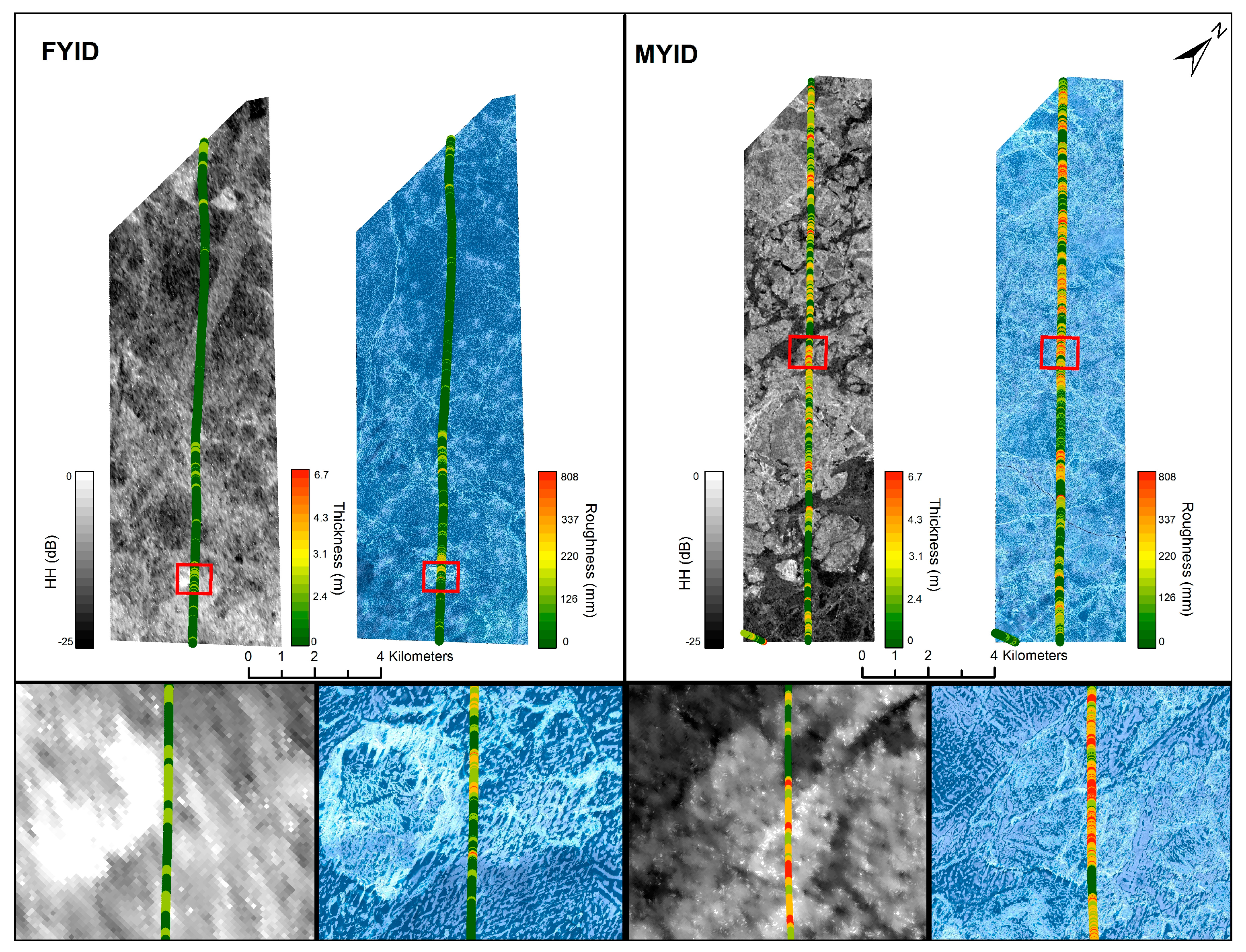
Figure 4.
Methods flow chart of RS-2 and GeoEye-1 image processing, segmentation, data aggregation, and correlation and regression analyses. The calibrated, speckle filtered and georeferenced RS-2 SAR image was segmented into image objects, with the objects used for further OBIA data aggregation. The objects were also reduced in across-track width to 120 m to create hybrid objects.
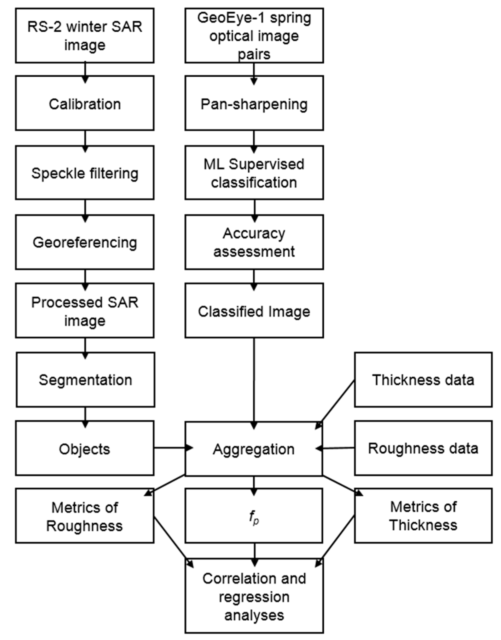
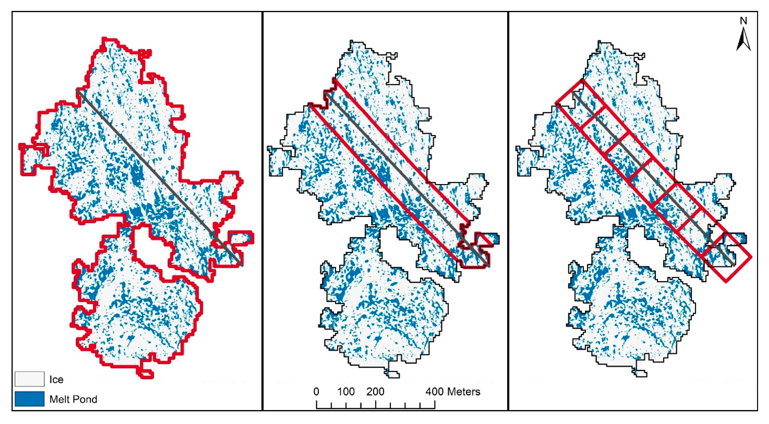
Figure 5.
Example comparison of object (left), hybrid (middle) and grid-cell (right) data aggregation approaches. The left panel shows an example of a MYI object (outlined in red), which represents a homogeneous ice zone overlaid on the fp product. The fp product shows melt pond pixels in blue, and ice pixels in white. The gray line represents the track of thickness and roughness data, which intersects the object. Similarly, the middle panel shows a hybrid object (outlined in red) and the right panel shows 120 × 120 m grid-cells centered on the thickness/roughness track. The hybrid objects were created to account for the footprints of the thickness and roughness sensors.

Figure 6.
Winter sea ice surface roughness (top left), smoothed surface roughness (top right), winter sea ice thickness (bottom left) and spring fp (bottom right) distributions. FYI is shown in blue and MYI in red. Mean (μ) and standard deviations (σ) are given by ice type. fp distributions were calculated using hybrid-object aggregation at the medium scale.

Figure 7.
Scatter plots of fp as a function of mean thickness at the medium scale using object (left), hybrid object (middle) and 240 m grid-cell (right) aggregation approaches. Spearman correlation coefficients (rs) and corresponding p-values are shown for pooled FYI and MYI data.
Figure 7.
Scatter plots of fp as a function of mean thickness at the medium scale using object (left), hybrid object (middle) and 240 m grid-cell (right) aggregation approaches. Spearman correlation coefficients (rs) and corresponding p-values are shown for pooled FYI and MYI data.

Figure 8.
A rational function OLS model of fp as a function of mean thickness. The data were aggregated using the hybrid-based approach at the medium scale. A rational function has been fitted to the data (solid blue line), with a 95% confidence interval (dashed blue line).
Figure 8.
A rational function OLS model of fp as a function of mean thickness. The data were aggregated using the hybrid-based approach at the medium scale. A rational function has been fitted to the data (solid blue line), with a 95% confidence interval (dashed blue line).
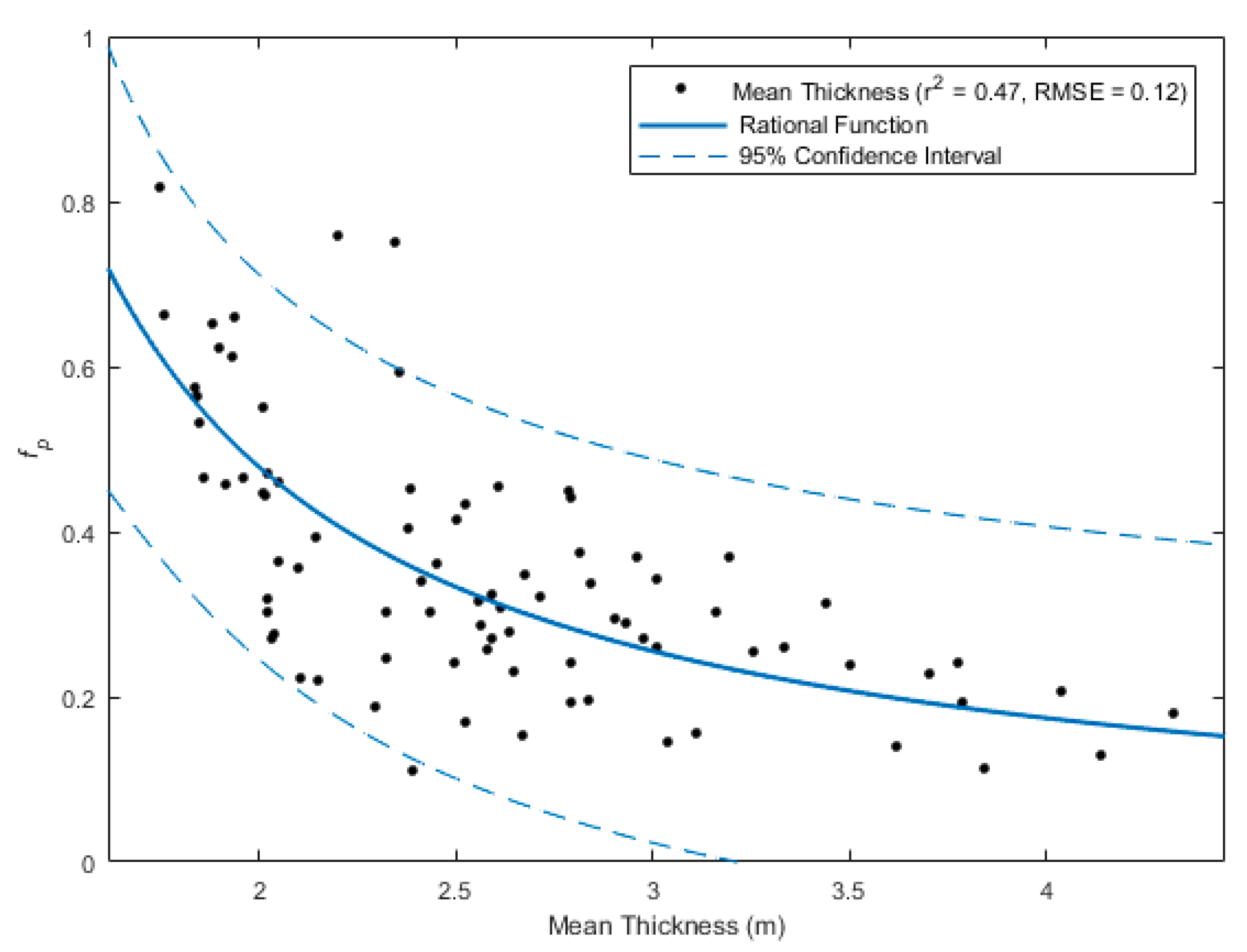
Figure 9.
Scatter plots of fp as a function of standard deviation of roughness at the medium scale using object (left), hybrid object (middle) and 240 m grid-cell (right) aggregation approaches. Spearman correlation coefficients (rs) and corresponding p-values are shown for pooled FYI and MYI data.
Figure 9.
Scatter plots of fp as a function of standard deviation of roughness at the medium scale using object (left), hybrid object (middle) and 240 m grid-cell (right) aggregation approaches. Spearman correlation coefficients (rs) and corresponding p-values are shown for pooled FYI and MYI data.

Figure 10.
Linear OLS model of fp as a function of standard deviation of roughness. The data was aggregated using the hybrid-based approach at the medium scale. A linear function has been fitted to the data (solid blue line), with a 95% confidence interval (dashed blue line).
Figure 10.
Linear OLS model of fp as a function of standard deviation of roughness. The data was aggregated using the hybrid-based approach at the medium scale. A linear function has been fitted to the data (solid blue line), with a 95% confidence interval (dashed blue line).
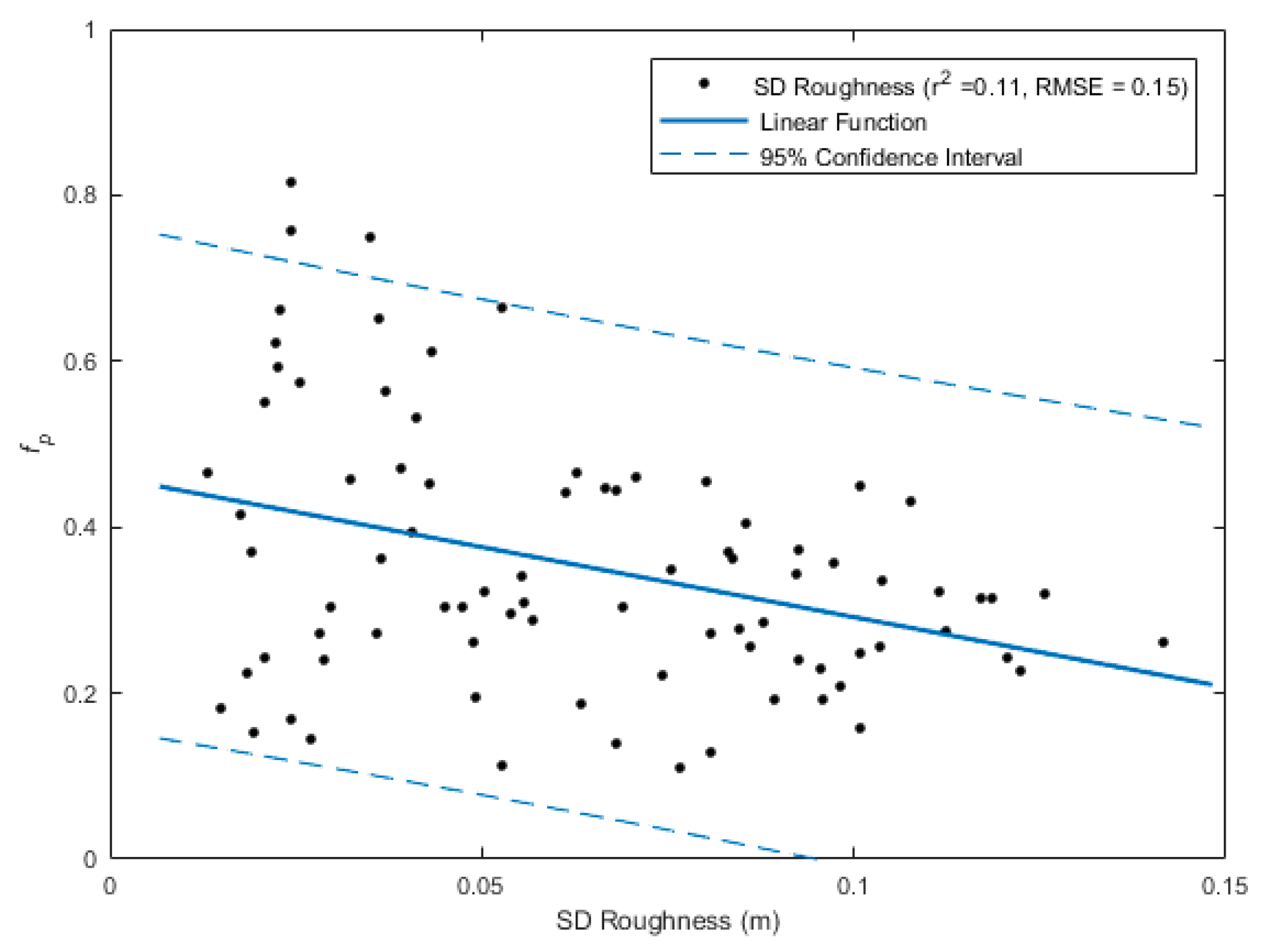
Figure 11.
Scatter plots of fp as a function of smoothed minimum surface roughness at the medium scale using object (left), hybrid object (middle) and 240 m grid-cell (right) aggregation approaches. Spearman correlation coefficients (rs) and corresponding p-values are shown for pooled FYI and MYI data.
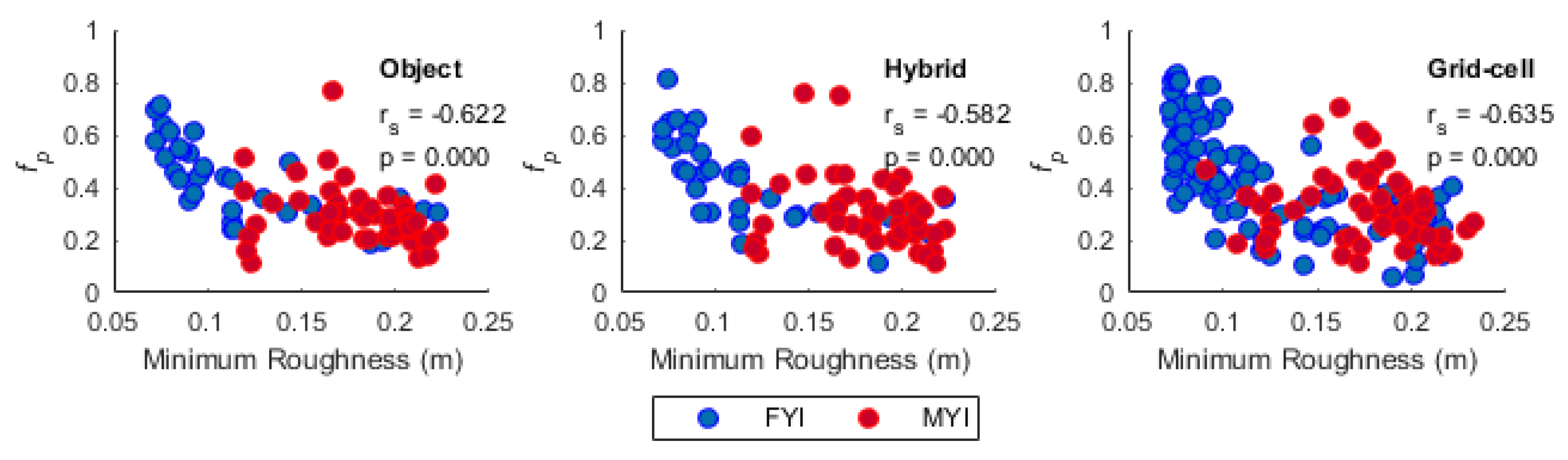
Figure 12.
Scatter plots of maximum roughness as a function of maximum thickness at the medium scale using object (left) and 240 m grid-cell (right) aggregation approaches. Spearman correlation coefficients (rs) and corresponding p-values are shown for pooled FYI and MYI data.
Figure 12.
Scatter plots of maximum roughness as a function of maximum thickness at the medium scale using object (left) and 240 m grid-cell (right) aggregation approaches. Spearman correlation coefficients (rs) and corresponding p-values are shown for pooled FYI and MYI data.
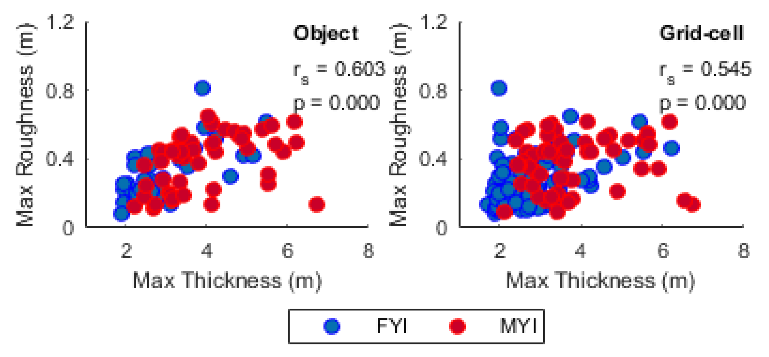
Figure 13.
2016 snow depth distributions on FYI (blue) and MYI (red) near Eureka in the CAA. Mean (μ) and standard deviations (σ) are given by ice type. 1792 measurements snow depth measurements were collected on FYI and 1810 measurements on MYI.
Figure 13.
2016 snow depth distributions on FYI (blue) and MYI (red) near Eureka in the CAA. Mean (μ) and standard deviations (σ) are given by ice type. 1792 measurements snow depth measurements were collected on FYI and 1810 measurements on MYI.

Table 1.
Description of the datasets.
| Parameter | Instrument | Measurement Approach | Platform | Acquisition Dates | Description |
|---|---|---|---|---|---|
| Snow plus Ice Thickness | EM-bird | Electromagnetic induction and laser altimeter | Airborne | 19 April 2015 | Spatial resolution: 6.0 m Swath width: ~120 m Accuracy: 0.15 m |
| Ice Surface Roughness | Riegel Laser Measurement System Q120 | 2D laser scanner | Airborne | 19 April 2015 | Spatial resolution: 1.2 m Swath width: 105 m Accuracy: 0.025 m |
| Melt Pond Fraction (fp) | GeoEye-1 | Multispectral (VIS/NIR) | Satellite | 22 June 2015 23 June 2015 25 June 2015 | Spatial resolution: Panchromatic (0.5 m), Multispectral (2.0 m) Spectral resolution: RGBNIR |
| Objects | RADARSAT-2 | C-band frequency SAR | Satellite | 23 April 2015 25 April 2015 | 23 April 2015 Pixel Spacing (azimuth × range): 5.1 × 4.7 m Incidence angle: 40.2°–41.6° Polarization: Fine Quad 25 April 2015 Pixel spacing (azimuth × range): 4.9 × 4.7 m Incidence angle: 22.3°–24.2° Polarization: Fine Quad |
Table 2.
Spearman correlation coefficients (rs) between metrics of winter sea ice thickness and spring fp for FYI and MYI at fine, medium (med) and coarse spatial scales (object and hybrid) as well as 120 and 240 m grid-cells. Bolded values are statistically significant (p < 0.05).
Table 2.
Spearman correlation coefficients (rs) between metrics of winter sea ice thickness and spring fp for FYI and MYI at fine, medium (med) and coarse spatial scales (object and hybrid) as well as 120 and 240 m grid-cells. Bolded values are statistically significant (p < 0.05).
| FYI | MYI | FYI | MYI | FYI | MYI | ||||||||||||
|---|---|---|---|---|---|---|---|---|---|---|---|---|---|---|---|---|---|
| Fine | Med | Fine | Med | Coarse | Fine | Med | Fine | Med | Coarse | 120 m | 240 m | 120 m | 240 m | ||||
| Min | Objects | −0.66 | −0.61 | −0.37 | −0.33 | −0.31 | Hybrid | −0.64 | −0.67 | −0.32 | −0.27 | −0.31 | Grid-cell | −0.61 | −0.65 | −0.30 | −0.11 |
| Max | −0.51 | −0.67 | −0.45 | −0.33 | −0.29 | −0.40 | −0.73 | −0.43 | −0.42 | −0.40 | −0.72 | −0.75 | −0.46 | −0.38 | |||
| Mean | −0.72 | −0.75 | −0.59 | −0.54 | −0.56 | −0.68 | −0.85 | −0.55 | −0.56 | −0.59 | −0.71 | −0.75 | −0.47 | −0.41 | |||
| Med | −0.75 | −0.71 | −0.60 | −0.56 | −0.58 | −0.74 | −0.81 | −0.59 | −0.60 | −0.64 | −0.69 | −0.75 | −0.45 | −0.44 | |||
| SD | −0.38 | −0.65 | −0.36 | −0.25 | −0.25 | −0.31 | −0.72 | −0.32 | −0.32 | −0.34 | −0.60 | −0.69 | −0.47 | −0.38 | |||
Table 3.
Spearman correlation coefficients (rs) between metrics of winter sea ice roughness and spring fp for FYI and MYI at fine, medium (med) and coarse spatial scales (object and hybrid) as well as 120 and 240 m grid-cells. Bolded values are statistically significant (p < 0.05).
Table 3.
Spearman correlation coefficients (rs) between metrics of winter sea ice roughness and spring fp for FYI and MYI at fine, medium (med) and coarse spatial scales (object and hybrid) as well as 120 and 240 m grid-cells. Bolded values are statistically significant (p < 0.05).
| FYI | MYI | FYI | MYI | FYI | MYI | ||||||||||||
|---|---|---|---|---|---|---|---|---|---|---|---|---|---|---|---|---|---|
| Fine | Med | Fine | Med | Coarse | Fine | Med | Fine | Med | Coarse | 120 m | 240 m | 120 m | 240 m | ||||
| Min | Objects | −0.34 | −0.32 | 0.30 | 0.21 | 0.16 | Hybrid | −0.35 | −0.31 | 0.25 | 0.27 | 0.19 | Grid-cell | −0.25 | −0.26 | −0.05 | −0.01 |
| Max | −0.29 | −0.57 | 0.01 | 0.05 | 0.07 | −0.20 | −0.53 | 0.02 | 0.04 | 0.01 | −0.40 | −0.55 | −0.10 | −0.12 | |||
| Mean | −0.32 | −0.53 | 0.02 | 0.03 | −0.02 | −0.25 | −0.52 | 0.04 | 0.09 | 0.00 | −0.35 | −0.42 | −0.09 | −0.11 | |||
| Med | −0.22 | −0.41 | −0.03 | 0.00 | −0.07 | −0.14 | −0.36 | 0.03 | 0.06 | −0.03 | −0.30 | −0.37 | −0.07 | −0.11 | |||
| SD | −0.35 | −0.59 | −0.07 | −0.03 | −0.02 | −0.29 | −0.63 | 0.00 | −0.01 | −0.06 | −0.39 | −0.54 | −0.10 | −0.17 | |||
Table 4.
Spearman correlation coefficients (rs) between metrics of smoothed winter sea ice roughness and fp for FYI and MYI at fine, medium (med) and coarse spatial scales. The data were aggregated using the hybrid object aggregation approach. Bolded values are statistically significant (p < 0.05).
Table 4.
Spearman correlation coefficients (rs) between metrics of smoothed winter sea ice roughness and fp for FYI and MYI at fine, medium (med) and coarse spatial scales. The data were aggregated using the hybrid object aggregation approach. Bolded values are statistically significant (p < 0.05).
| FYI | MYI | FYI | MYI | FYI | MYI | ||||||||||||
|---|---|---|---|---|---|---|---|---|---|---|---|---|---|---|---|---|---|
| Fine | Med | Fine | Med | Coarse | Fine | Med | Fine | Med | Coarse | 120 m | 240 m | 120 m | 240 m | ||||
| Min | Objects | −0.81 | −0.80 | −0.31 | −0.35 | −0.34 | Hybrid | −0.77 | −0.84 | −0.34 | −0.29 | −0.25 | Grid-cell | −0.72 | −0.77 | −0.20 | −0.23 |
| Max | −0.79 | −0.81 | −0.27 | −0.26 | −0.21 | −0.72 | −0.80 | −0.24 | −0.19 | −0.09 | −0.72 | −0.77 | −0.19 | −0.22 | |||
| Mean | −0.80 | −0.81 | −0.29 | −0.29 | −0.27 | −0.75 | −0.83 | −0.28 | −0.23 | −0.17 | −0.72 | −0.77 | −0.19 | −0.22 | |||
| Med | −0.80 | −0.81 | −0.29 | −0.29 | −0.26 | −0.75 | −0.82 | −0.26 | −0.22 | −0.16 | −0.72 | −0.77 | −0.19 | −0.22 | |||
| SD | −0.14 | −0.34 | 0.06 | 0.24 | 0.28 | −0.04 | −0.23 | 0.17 | 0.19 | 0.26 | −0.45 | −0.55 | 0.08 | 0.01 | |||
Table 5.
Spearman correlation coefficients (rs) between metrics of winter sea ice roughness and thickness for FYI and MYI at fine, medium (med) and coarse spatial scales (object) as well as 120 and 240 m grid-cells. Bolded values are statistically significant (p < 0.05).
Table 5.
Spearman correlation coefficients (rs) between metrics of winter sea ice roughness and thickness for FYI and MYI at fine, medium (med) and coarse spatial scales (object) as well as 120 and 240 m grid-cells. Bolded values are statistically significant (p < 0.05).
| FYI | MYI | FYI | MYI | ||||||||
|---|---|---|---|---|---|---|---|---|---|---|---|
| Fine | Med | Fine | Med | Coarse | 120 m | 240 m | 120 m | 240 m | |||
| Min | Objects | 0.39 | 0.36 | 0.07 | 0.21 | 0.27 | Grid-cell | 0.30 | 0.34 | 0.01 | 0.23 |
| Max | 0.56 | 0.65 | 0.41 | 0.54 | 0.57 | 0.44 | 0.53 | 0.11 | 0.13 | ||
| Mean | 0.36 | 0.49 | 0.20 | 0.20 | 0.23 | 0.41 | 0.44 | 0.07 | 0.07 | ||
| Med | 0.18 | 0.26 | 0.12 | 0.06 | 0.03 | 0.34 | 0.38 | 0.04 | 0.13 | ||
| SD | 0.52 | 0.68 | 0.40 | 0.47 | 0.47 | 0.35 | 0.45 | 0.05 | 0.07 | ||
© 2017 by the authors. Licensee MDPI, Basel, Switzerland. This article is an open access article distributed under the terms and conditions of the Creative Commons Attribution (CC BY) license (http://creativecommons.org/licenses/by/4.0/).
Share and Cite
MDPI and ACS Style
Nasonova, S.; Scharien, R.K.; Haas, C.; Howell, S.E.L. Linking Regional Winter Sea Ice Thickness and Surface Roughness to Spring Melt Pond Fraction on Landfast Arctic Sea Ice. Remote Sens. 2018, 10, 37. https://doi.org/10.3390/rs10010037
AMA Style
Nasonova S, Scharien RK, Haas C, Howell SEL. Linking Regional Winter Sea Ice Thickness and Surface Roughness to Spring Melt Pond Fraction on Landfast Arctic Sea Ice. Remote Sensing. 2018; 10(1):37. https://doi.org/10.3390/rs10010037
Chicago/Turabian StyleNasonova, Sasha, Randall K. Scharien, Christian Haas, and Stephen E. L. Howell. 2018. "Linking Regional Winter Sea Ice Thickness and Surface Roughness to Spring Melt Pond Fraction on Landfast Arctic Sea Ice" Remote Sensing 10, no. 1: 37. https://doi.org/10.3390/rs10010037
Note that from the first issue of 2016, this journal uses article numbers instead of page numbers. See further details here.