Quantification of Two-Dimensional Wave Breaking Dissipation in the Surf Zone from Remote Sensing Data


1
Departamento de Obras Civiles, Universidad Técnica Federico Santa María, Valparaíso, Chile
2
Centro Nacional de Investigación para la Gestión Integrada de Desastres Naturales, CONICYT/FONDAP/1511007, Santiago, Chile
3
CCTVal-Centro Científico Tecnológico de Valparaíso, Valparaíso, Chile
4
College of Earth, Oceanic and Atmospheric Sciences, Oregon State University, Corvallis, OR 97331, USA
*
Author to whom correspondence should be addressed.
†
These authors contributed equally to this work.
Remote Sens. 2018, 10(1), 38; https://doi.org/10.3390/rs10010038
Submission received: 30 October 2017
/
Revised: 20 December 2017
/
Accepted: 21 December 2017
/
Published: 26 December 2017
(This article belongs to the Special Issue Instruments and Methods for Ocean Observation and Monitoring)
Abstract
:A method for obtaining two dimensional fields of wave breaking energy dissipation in the surfzone is presented. The method relies on acquiring geometrical parameters of the wave roller from remote sensing data. These parameters are then coupled with a dissipation model to obtain time averaged two dimensional maps, but also the wave breaking energy dissipation on a wave-by-wave basis. Comparison of dissipation maps as obtained from the present technique and a results from a numerical model, show very good correlation in both structure and magnitude. The location of a rip current can also be observed from the field data. Though in the present work a combination of optical and microwave data is used, the underlying method is independent of the remote sensor platform. Therefore, it offers the possibility to acquire high quality and synoptic estimates that could contribute to the understanding of the surfzone hydrodynamics.
1. Introduction
The nearshore is the narrow portion of the oceans in contact with continental land. Despite its relatively limited extent, it is an extremely dynamic area where hydrodynamic and morphodynamic process interact over a wide range of temporal and spatial scales. At the same time, it is one of the areas most dear to humans, for reasons that span from recreational to economic activities. A predictive understanding of the nearshore is relevant for many aspects of human endeavors.
Essential to this understanding are nearshore hydrodynamic processes. Although several temporal and spatial scales can be considered, nearshore hydrodynamics are strongly influenced by processes at the time scale of surface gravity waves. Key among these is the dissipation of wave energy, which results not only in the attenuation of waves as they propagate, but also transfers momentum from the wave organized motion to wave-induced mean quantities. These include both forcing of mean flows, i.e., currents and circulation patterns (e.g., [1]), and changes in mean water levels (e.g., [2,3]). The importance of wave energy dissipation led Holman and Haller [4] to argue that a direct measurement of wave energy dissipation is equivalent to measuring the mean flow forcing in the nearshore. Therefore, a robust methodology to estimate wave energy dissipation can be instrumental in improving our understanding of this environment. In this context, remote sensing techniques can play a key role.
In what follows, the term dissipation is used to denote wave breaking energy dissipation, unless noted otherwise. Although dissipation is due to several processes, the most relevant in the nearshore is wave breaking, which transfers organized wave motion into motion at several scales and types [5]. In the nearshore, the most relevant component of dissipation is depth-limited breaking, which can occur in several regimes (plunging, collapsing, spilling, and surging). However, a typical approach in modeling breaking dissipation relies upon estimating total dissipation by a canonical broken wave [6], often by establishing analogies with similar known flows such as bores or hydraulic jumps (e.g., [6,7]). These form key parameterizations in nearshore ocean models that do not directly resolve short wave forcing (e.g., [8,9]), and can help to validate models which do resolve waves but not the wave dissipation process itself (e.g., [10,11,12]). In the inner surf zone, breaking waves become bore-like and the wave roller, the turbulent body of air and water that propagates with the breaking wave, is considered the feature of dynamical interest, controlling the energy flux, radiation stresses and dissipation [13,14].
Thus, quantifying the evolution of rollers can be relevant for estimating dissipation. The signal of the roller is prominent in many remote sensing modalities, such as passive acoustic (e.g., [15]), optical (e.g., [16]), microwave (e.g., [17]), and infrared (e.g., [18]). Moreover, a wide range of platforms can be used to deploy the sensors, from nearshore towers and antennas (e.g., [4], for a review) to satellites (e.g., [19]). One important advantage of remote sensing measurements is that they can be synoptic and have large spatial coverage, although roller identification does require ad hoc procedures and algorithms. It is of note also that success in identifying the occurrence of the wave roller does not provide a direct estimate of wave breaking energy dissipation, rather a model is needed. A relatively simple formulation to estimate the roller induced dissipation relies on a relationship between local geometrical parameters such as the wave height and the roller cross-sectional area A [20,21,22,23]. Some of these parameters can be inferred by a range of remote sensing modalities, which have allowed the estimation of the local dissipation due to wave breaking, under the assumption that roller induced dissipation is the dominant mechanism [24,25,26]). Flores et al. [27] followed on these ideas and estimated the one-dimensional forcing of the mean water level (i.e., wave setup) by coupling estimates of wave breaking dissipation (from remote sensing) and a phase averaged model based on the roller formulation. The results showed that including the remotely sensed roller estimates improved estimation of wave setup.
One notable aspect to all these recent roller-related efforts is that they assume a one-dimensional (across-wave) wave breaking geometry. The main reason is that wave energy dissipation takes place essentially in the direction of wave propagation, therefore analysis along the wave ray is straightforward. However, in the surfzone, waves can have different propagation directions due to multimodal sea states and/or non-uniform bathymetry. As a result, wave breaking can exhibit significant spatial variability. Thus, it is desirable to extend existing methods to quantify the two dimensional dissipation field. However, achieving this requires at a minimum a detailed wave-by-wave estimation of wave breaking occurrence. Hence, a necessary first step in quantifying wave breaking dissipation is the identification of the active breaking wave, and several remote sensing regimes can provide the requisite level of spatial and temporal coverage. In particular, it is expected that data collection should provide spatial coverage of several wavelengths and span the surfzone, along with enough alongshore coverage to capture the spatial variability of interest. At the same time, spatial resolution should be sufficient to capture the planform geometry of the wave roller (owing to the model dependency described above). Temporal resolution should be sufficient to track waves as they propagate throughout the surfzone, which typically requires sampling rates of at least 2 Hz. A suite of remote sensing modalities such as electro optical (video), infrared, or microwave, can provide data satisfying these requirements. It must be noted, however, that individual sensors can be subject to false alarms because the signal of interest can have a similar value to other spurious sources. For example, for optical sensors, active breaking can be difficult to separate from remnant foam, yet only the former is of dynamic interest [4,16]. Catalán et al. [28] successfully used sensor combination to overcome this difficulty.
One troubling aspect is how to validate proposed methods to quantify dissipation. In situ data do not measure dissipation directly, but typically rely on the estimation of the gradient of the wave energy flux via an across-shore array of wave height gages, with the assumption that an accurate prediction of the wave height profile yields a proper estimation of dissipation (e.g., [6,29]). More recently, Turbulent Kinetic Energy dissipation rates have been estimated locally or from drifters [30], and used to compare against roller-derived dissipation [26]. However, comparisons are only available locally, or along transects. A more complex approach was used by Clark et al. [31], who measured the mean rate of vorticity generation and related it to the dissipation force. This method is less direct, and requires a dense array of sensors. Finally, a wide range of numerical models can predict dissipation, either phase averaged (e.g., SWAN [32]) or phase resolving (e.g., Boussinesq [33,34] among many others). Any of these could be used to compare model dissipation output against observations for a preliminary assessment.
In this work, the algorithmic basis to estimate 2D wave breaking energy dissipation fields in the surfzone from remote sensing data is presented. While the methodology proposed by Catalán et al. [28] to identify active breaking is used herein, the fundamental approach used can be applied to any remote sensing technique capable to discriminate active breaking from other wave stages. A roller model [13,14] is used to estimate the local dissipation on a wave-by-wave basis. As a result, dissipation maps are obtained directly from remote sensing data without the need to other information such as input wave conditions nor bathymetry. Owing to inherent difficulties in validating the results, both qualitative and quantitative assessments are presented, in the form of comparing estimates of dissipation from data produced herein and those provided by numerical modeling.
2. Methods
2.1. Wave Breaking Identification and Tracking
Within the scope of the present work, it is understood that although the wave breaking discrimination procedure could be sensor dependent, the overall methodology to derive two dimensional wave breaking energy dissipation can be assumed to hold for a range of remote sensing techniques. In what follows, the method proposed by Catalán et al. [28] is used for reference, and it is described briefly for completeness.
Catalán et al. [28] take advantage of the signal characteristics of two remote sensing instruments, working in the electro optical and microwave range (at X-band), respectively. In Figure 1a,b, sample snapshots of marine radar and video data are presented. It can be seen that in both sensors, high backscatter and optical intensity (brighter areas) can be obtained within the surfzone. Optical (henceforth video) data include high intensity returns for both remnant foam and rollers. Microwave data (radar) at this frequency range can yield high backscatter intensities for both steepening and breaking waves [17]. However, foam and steepening waves rarely co-occur. Hence, the combination of radar and video signals allows for isolating active breaking occurrence in the nearshore. To do this, the probability density function (pdf) of intensity data from each sensor, and their joint probability density function (jpdf) are computed over a field of view (FOV) spanning either the entire image, or a subset of it. The use of smaller FOVs are recommended when wave breaking has large variability over the entire FOV. The individual pdfs show inflexion points that allow establishing thresholds (red lines in panel d,f in Figure 1) separating zones of low intensity to high intensity. These are passed on to the jpdf to identify four combinations associated with different wave stages: Active breaking (large video intensity and large radar return); remnant foam (large video intensity and low radar return); steepening waves (low video intensity and large radar return); and non breaking waves (other cases). These thresholds are then used in the time domain to categorize each instance of data, allowing separation between wave stages. Figure 1c shows a sample result, where red, cyan and green dots represent active breaking, remnant foam and steepening waves, respectively. More details on the procedure can be found in [28].
The selection of thresholds in this work has been updated from the subjective method used by Catalán et al. [28], by adapting the automatic threshold selector proposed by Carini et al. [26]. The slope and curvature of the pdf are calculated by
where pdf, pdf, pdf represent the probability density function, its first and second order discrete derivatives, respectively. S represents a signal intensity, in the present case either video optical intensity (I), or radar backscattering radar normalized cross-sections (, in dB). correspond to the intensity discretization steps used to construct the pdf.
The initial step is to identify a local minimum at intensities larger than that corresponding to the peak of the pdf
where is the threshold intensity selected, and is the intensity where the pdf has its maximum value. The presence of a local minimum suggests that a second peak, at higher intensities, is present in the pdf. However, if no local minimum are found (thus a monotonic decrease in the pdf), the maximum curvature is used
which is indicative of a change in the behavior of the pdf. This situation can occur for adverse weather conditions like the presence of fog or excessive foam production (e.g., [26,28]).
Finally, a hard-coded lower limit is imposed on the thresholds, based on the expected range of intensities associated with breaking waves for each sensor. If the above procedure yields video intensities thresholds outside of the range , the algorithm automatically assigns it as , where is the maximum pixel intensity of the time exposure. Catalán et al. [28] found this value to be consistent with their manually selected thresholds. Although this rule eventually could yield values that can be considered too low, Haller and Catalán [24] found that roller fronts are characterized by a sharp gradient in pixel intensity, making them distinguishable and less dependent on threshold value. In the case of the marine radar, if is outside of the range dB, the algorithm automatically assigns either limit. It must be noted that, in general, these values may vary among different locations and grazing angles. For the present case, they have been derived by Catalán et al. [17].
With this procedure, a time series of images are obtained containing multiple areas of active breaking. Since intensity information is not directly related to dissipation, a binary image is created for each frame identifying the locations of active wave breaking. This step allows the algorithm that follows to be applied in principle to any remote sensing platform capable of detecting active breaking.
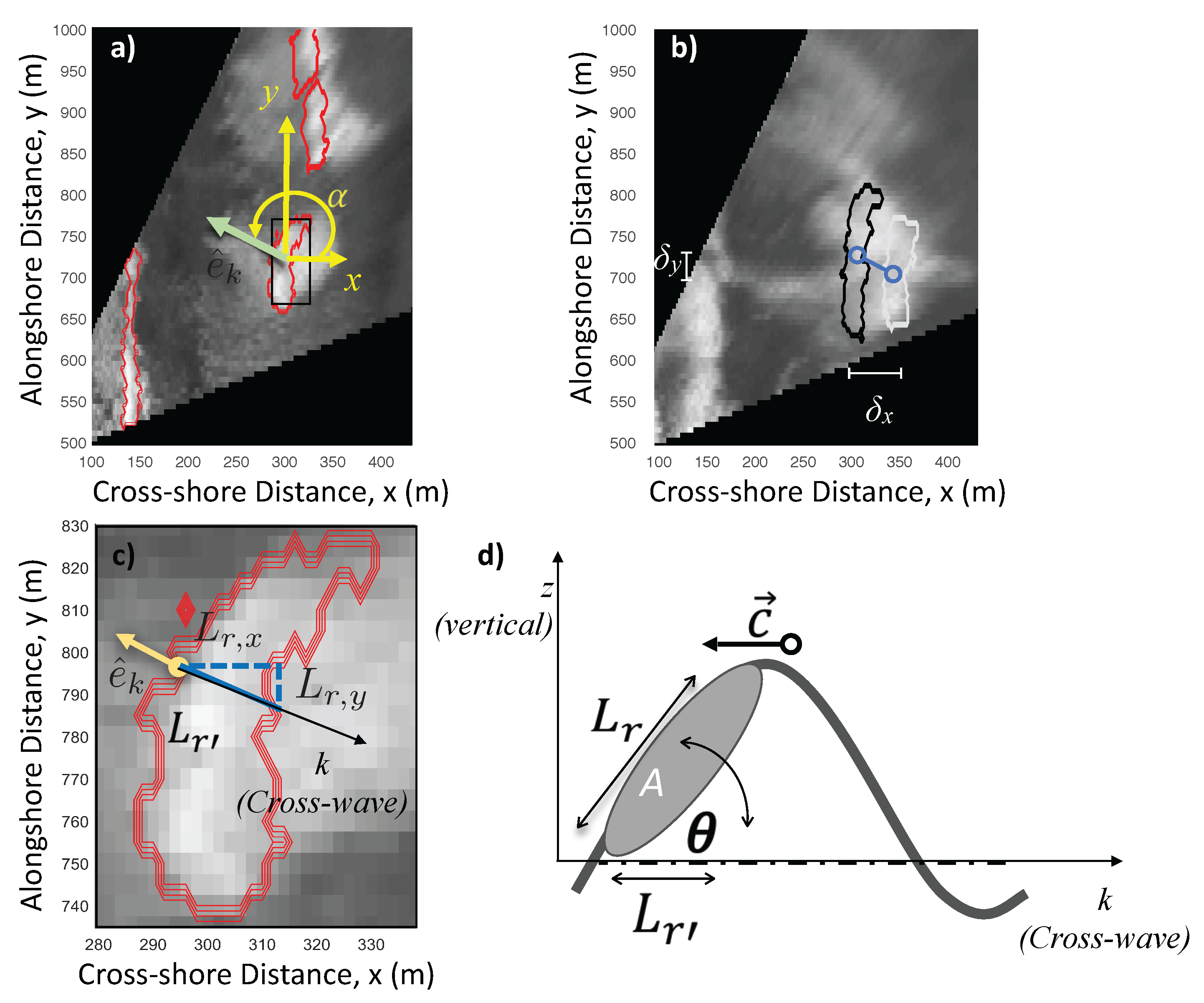
Several rollers may be present simultaneously on each frame, and it is required to track each one of them in space and time to obtain the Lagrangian history of each individual breaking event. This allows estimation of their propagation angle, event duration and the rate of events occurring on each frame. Owing to the possibility of waves and rollers traveling in different directions, all information is recorded in a global Cartesian coordinate system, in this case aligned with the cross-shore and alongshore directions, as shown in Figure 2a. To track a given roller in time, two breaking areas present at consecutive frames are considered to be the same roller if their centroids propagate at a velocity smaller than a threshold value m/s, where and are the components of the wave celerity vector for user-prescribed nominal values of water depth and wave period.
Once such a roller has been identified in consecutive frames, its propagation angle is estimated as
where are the cross-shore and alongshore components of the displacement vector of the centroid, as shown in Figure 2a,b. Note, corresponds to cross-shore propagating waves in the global reference system used here.
The tracking technique allows book-keeping relevant information of the roller evolution as it propagates throughout the surf zone. These include the propagation angle, roller area and across-wave length, which are relevant parameters in the dissipation model.
2.2. Dissipation Estimation
Once all of the roller instances have been recorded, local dissipation values can be computed for each. It is assumed that all of the wave breaking energy dissipation arises from the roller. Duncan [13] proposed a model for wave breaking dissipation due to rollers in equilibrium (henceforth ), in which dissipation is the result of the work done by shear stress acting on the interface between the roller and the underlying wave. This shear stress must balance the weight of the roller for the latter to remain in its position relative to the wave. Hence, the time-averaged rate of dissipation per unit planform area in the direction of wave motion reads [13,23,35]
where is the average density of the roller (here assumed constant and equal to 60% of the sea water density, following Carini et al. [26]); A is the cross-sectional area of the roller; T is the wave period; and is the inclination angle of the roller relative to the horizontal, defined in a local reference frame propagating with the wave (see Figure 2c,d for reference). This angle affects the amount of wave energy storage in the roller as well as its size. Thus, the energy dissipation is controlled by the wave roller geometry. observed that the roller geometry is self-similar through most of its life cycle
where is the along-slope length of the roller. Assuming is known and equivalent to the angle of the front face of the wave, it is possible to relate the horizontal projection of , as . Hence, a local (in space and time), estimate of the dissipation can be obtained by estimating its horizontal projection and slope angle . Laboratory and field data broadly support this model, even though the premise of rollers in equilibrium does not necessarily hold. As a result, the only free parameter has been used as a tuning parameter (e.g., [24,26,27]).
To estimate the dissipation fields, it is assumed that most of energy dissipation occurs in the front face of the wave and that, at each point of the wave front, the local dissipation can be estimated from its local roller length. Hence, rearranging Equations (6) and (7) yields
Although it is known that varies in time and space, as a first step it is approximated as time-independent and cross-shore constant. A space-differencing approach is used to find roller fronts and backs on each binary image, allowing estimation of , for each pixel along the wave front, for each wave, and at each time step. Collecting these results allows estimation of the two dimensional dissipation fields. As an additional step, it is possible to assign an orientation to the dissipation based on the direction of wave propagation, , where is the unit vector along the wavenumber direction (e.g., [1,36]). A similar approach is used in two dimensional Boussinesq models to account for wave breaking dissipation (e.g., [33,34]). A single value for the propagation angle is assumed to be representative of each roller.
3. Experimental Data
To test and validate the proposed methodology, data from two different field experiments at the U.S. Army Corp of Engineers Field Research Facility (FRF), Duck, NC have been used. The FRF coordinate system is used here, where the cross-shore coordinate is denoted as x and points offshore, the alongshore y axis points roughly 18 west from north, and z = 0 corresponds to the NADV29 vertical datum. For the data analyzed herein, the shoreline was located at approximately x = 90 (m). Two remote sensing techniques are used. The first was a single polarization (HH) marine radar (Si-Tex RADARpc-25.9) operating at 9.45 GHz. The radar antenna was mounted atop a 10-m tower near the north end of the FRF property (x = 17.4 (m), y = 971.4 (m) and z = 13.8 (m)). The marine radar is an active sensor with a 25-kW nominal power and 9-ft open array antenna that rotates at approximately 44 rpm (see [28] for details). The second remote sensing system comprised three optical cameras from the ARGUS III observing station (see [16] for details).
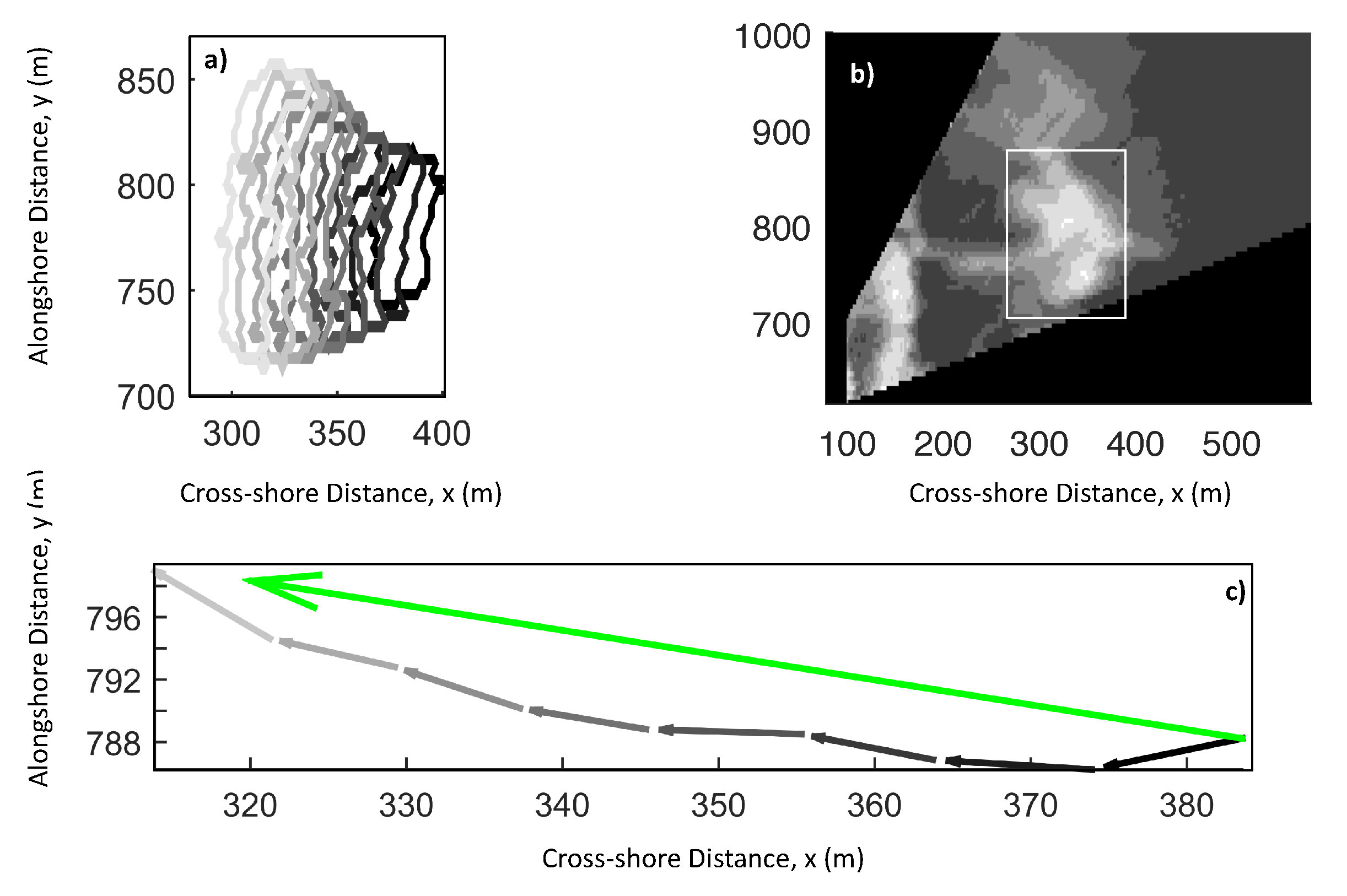
A regular pixel array is defined for data acquisition and post processing, spanning x = 60–600 (m) and y = 500–1000 (m), with a spatial resolution of m and m, using the FOV of cameras 0, 3 and 1, as shown in Figure 3 and Figure 4. To synchronize the two sensors, differences in sampling rates and spatial resolution were removed by interpolation to a common grid. Although we use three cameras of the ARGUS III system, boundaries between the cameras’ field of view have been avoided due the difference in gain leading to a sharp gradient not related with the ocean surface (see Figure 4, boundaries as dotted white lines).
The setup described above was used for two datasets from two experiments. The first dataset was taken from the Multi Remote SENsing Surfzone Observations (MR-SENSO) starting 14 May 2008 18:00 GMT with a duration of 27 min, hereinafter R1. The second dataset was taken from Surf Zone Optics Experiment (SZO) starting on 9 September 2010 17:59 GMT with a duration of 15 min, hereinafter R2. It is worth mentioning R2 was among those used by Haller et al. [37] to demonstrate that rip currents can be detected by microwave sensors. Wave conditions varied between the two datasets, from relatively energetic swell at mid tide, to a less energetic wind sea at low tide, as shown in Table 1. The environmental conditions of R2 were favorable for imaging the rip current, whereas no rip was present for R1. As can be seen in Figure 4, R1 had a wider surf zone with breaking over an offshore bar located at x = 250–350 m, consistent with more energetic conditions. R2 had a much narrower surf zone with concentrated breaking over a narrower bar located further onshore than that of R1. This bar included a narrow gap, near y = 800–850 m. Unfortunately, bathymetry was not surveyed regularly during MR-SENSO, whereas R2 had bathymetric surveys collected on 6 and 15 September 2010, using the specialized FRF vehicles LARC and CRAB.
4. Results
4.1. Breaking Detection
Without loss of generality, in what follows the focus is set on breaking within an area of interest defined by the offshore bars present in both cases. These areas are indicated by the green boxes in Figure 4. The thresholding algorithm yielded different values for each camera and case (see Table 2), whereas a constant value of dB was used for all cases. In addition, and were obtained from linear wave theory assuming a T = 10 s wave propagating in 10 m depth. This leads to expected displacements that are at most two pixels given the 2 Hz sampling rate.
As an example, the evolution of single event is shown in Figure 5. In Figure 5a, the cross-shore propagation of the event but also its lateral spreading and growth can be observed, which matches the average video intensity over the same time window (panel b). Figure 5c shows the frame-by-frame displacement of the centroid in red, whereas the green arrow shows the net change in position since wave breaking beginning. The centroid wobbles in the alongshore direction, due to the roller changing its size. However, these variations do not affect the overall propagation direction of the wave (i.e., ), which is the quantity of interest.
The total number of breaking events in R1 was 1740 (∼62 events per minute), and the average event duration was 6 s. On the other hand, R2 presented 1544 events (102 events per minute) with an average duration of 4 s. These results are consistent with the wave conditions observed, in the sense that the longer period waves of R1 break less frequently but have longer life spans than those in R2.
Analysis of the propagation angles obtained, performed over all individual events, shows a narrow normal distribution, with mean of 177 and 178, and standard deviations of 11 and 17, for R1 and R2, respectively (not shown). Both mean incidence angles are close to shore normal.
4.2. Roller Lengths and Dissipation Fields
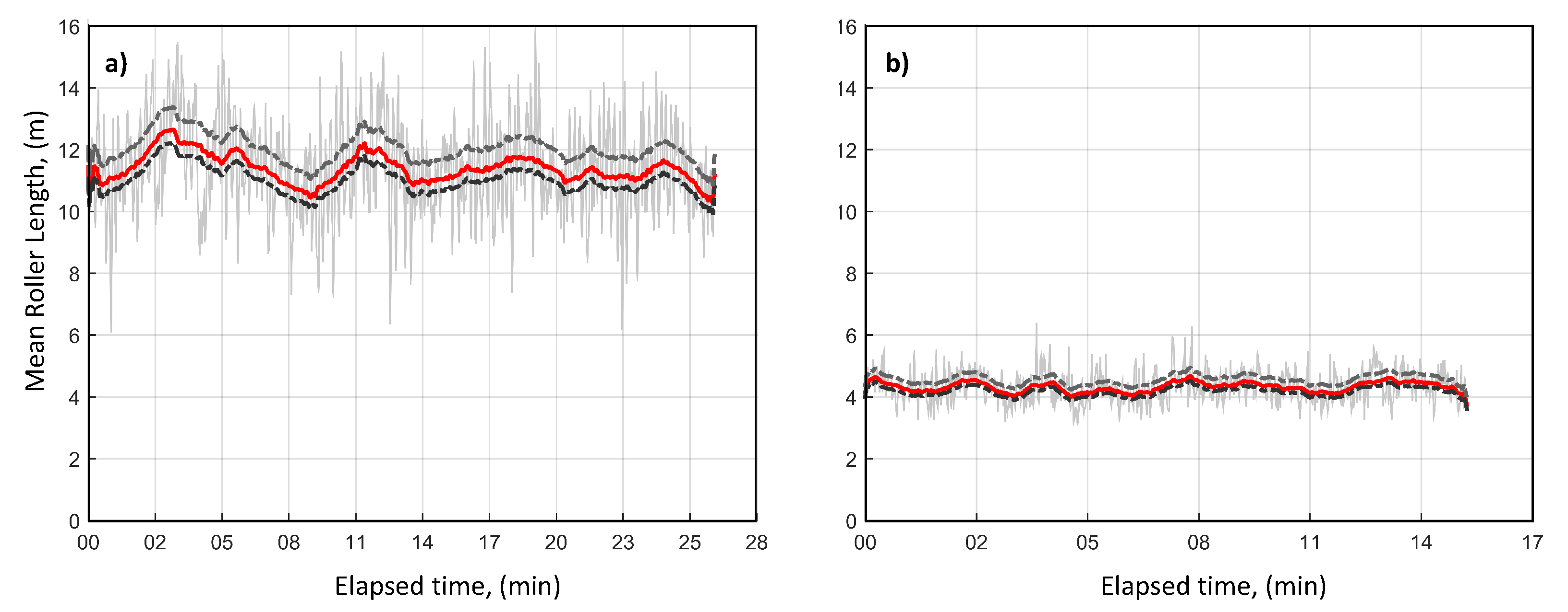
The average of the estimated roller lengths in R1 was 11 m, although the frame by frame mean value shows a large variability, as can be seen in Figure 6. On the other hand, R2 shows a shorter roller length with less variability but episodic peaks. Although there is no other method to estimate the roller length to compare against, a quick estimation shows that for waves in about 6 m water depth, these roller lengths represent less than one-eight of the total wavelength, which is generally consistent with the front face extent of periodic saw-tooth waves (e.g., [38]).
Although recently Zhang et al. [39] presented a parameterization for the front slope angle, here is assumed fixed with a value of 15 for both R1 and R2, consistent with the 2–24 range reported in the literature from both laboratory and field experiments [13,23,24,26,39,40,41]. In Figure 6, the mean roller length estimated using = 2 and 24 are also presented. It can be seen the nonlinear effect of dependency on the roller length, as the change in estimated lengths when changing from = 2 to 15 (13) is less than when changing from = 15 to 24 (9). As it will be discussed below, this is a relevant free parameter of the model which directly affects the dissipation estimates.
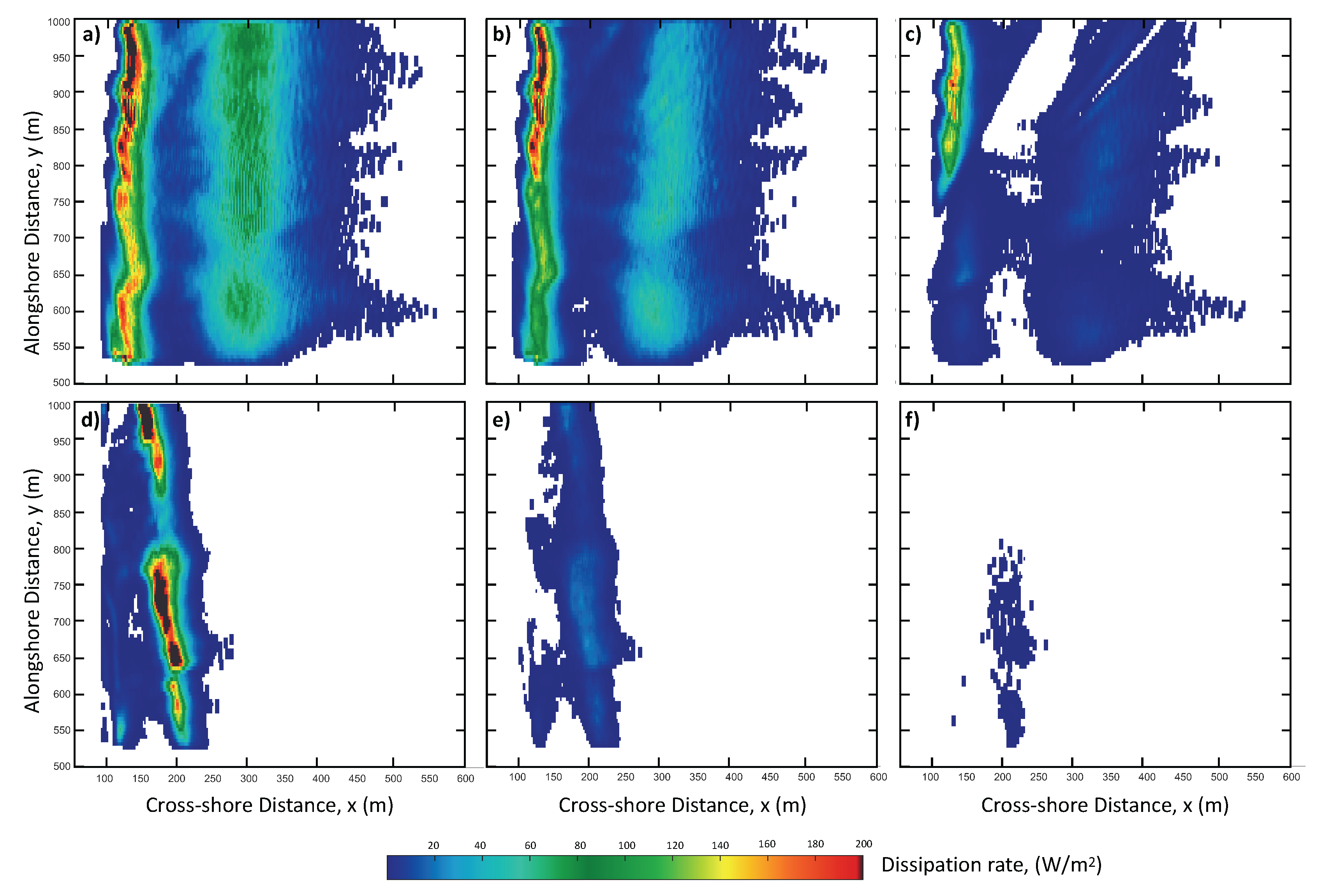
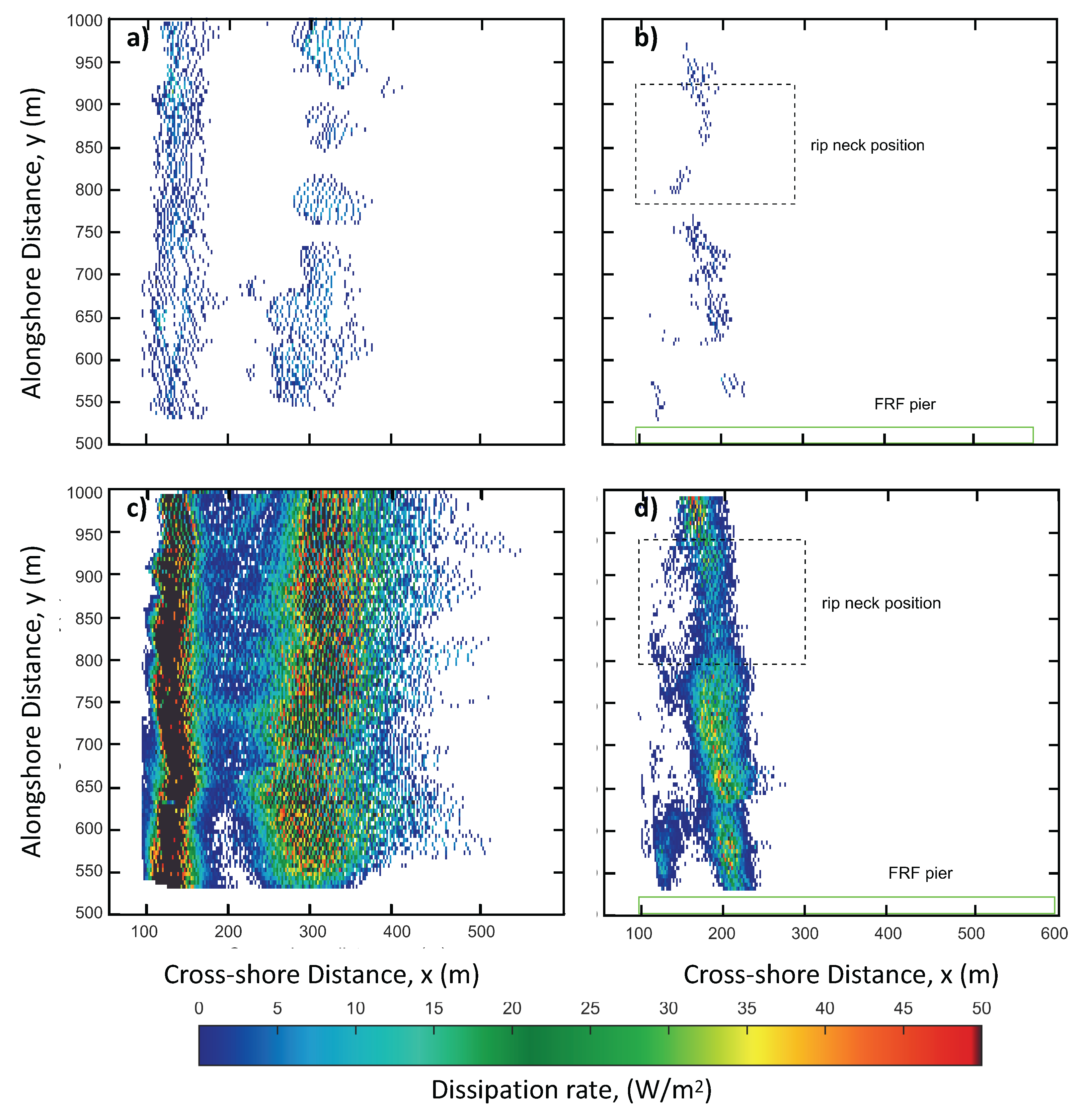
With the information collected, it is possible to construct spatio-temporal maps of wave breaking dissipation. A sample is seen in Figure 7 for R1 and R2 (left and right panels, respectively). While frame by frame wave breaking dissipation can be obtained, its a distribution has a patchy structure as the dissipation is concentrated at the wave fronts and these are sampled at 2 Hz. Therefore, dissipation maps are obtained by time-averaging the dissipation time series, to highlight the overall spatial structure. Figure 7a,b show averaging over , where individual events leave a clear dissipation track signature, and sharp gradients can be observed throughout the image owing to the noticeable tracking of individual events. Even so, it is possible to clearly distinguish breaking over the offshore bar from shoreline breaking, especially for R1 (Figure 7a). Moreover, offshore breaking leads to more energetic dissipation rates. Figure 7c,d show averaging over , where a more clearly defined structure becomes apparent. R1 shows an homogeneous dissipation structure over the sandbar, with no significant spatial gradients. Less dissipation was observed over the sandbar trough, and dissipation becomes significant near the shoreline due to more frequent breaking. In contrast, R2 shows a non-homogeneous behavior over the offshore sandbar, which creates large alongshore gradients specially in the range y = 800–950 (m). The reduced breaking at that location coincides with the rip neck position determined by Haller et al. [37], suggesting a possible correlation. The sharp gradient close to y = 600 m is an artifact of the camera boundary.
These results highlight that with the data collected, it is possible to estimate wave breaking dissipation (i.e., forcing ) not only over time scales of traditional time exposures used in nearshore applications ([4,16], typically 10 min), but also at the time scales of individual waves or wave groups. Thus, it offers the possibility to analyze the spatio-temporal evolution of nearshore forcing in more detail (e.g., [42]). It can also be noted that the spatial structures in both sets correlate well with the time-average image of video intensity (c.f. Figure 4). The latter has been previously considered as a potential proxy for dissipation [16]. The relevant difference is that unlike the time average of optical intensity, the present results have a physically meaningful dissipation estimate.
5. Discussion
5.1. Validation
The results presented above are encouraging, although its validation is challenging. This not only difficult because in situ data is required, but also because no other measuring technique is capable of producing spatial distributions of dissipation with the coverage and resolution as presented herein. Unfortunately, no other data were collected for R1, and in particular the bathymetry was not measured. On the other hand, bathymetry data were collected during SZO. In addition, modeling efforts have been carried out and verified for the period under analysis [43]. Therefore, a limited validation will be performed here by comparing the remote sensing measurements to model predictions for R2.
The model simulates depth- and time-averaged (over many wave periods) wave and roller energy propagation and the associated transfer of momentum from waves to mean currents. The model domain extends from the shoreline to m (∼8 m depth), and from to m, with grid spacing of 10 m cross-shore by 15 m alongshore. Periodic boundary conditions are used in the alongshore direction, and the northernmost 500 m of the model domain is used as an artificial buffer zone in which bathymetry is relaxed to be periodic. Bathymetry for the model is interpolated from measurements on 6 September 2010, only three days prior to the R2 data set.
The wave part of the model, SWAN, solves the stationary conservation of wave action equation [44], and is initialized at the offshore boundary with wave spectra derived from measurements by the FRF 8 m array [45] (assumed alongshore-uniform). Wave breaking dissipation is the only source/sink for wave energy, and is calculated following Battjes and Janssen [6], with SWAN-default parameters. The influence of low-frequency currents on waves is neglected. Finally, the SWAN outputs are passed to a wave roller evolution model [22], with roller face angle rad (6) chosen based on longshore current model calibration experiments (using the same roller formulation) for this site by Ruessink et al. [41].
The wave roller model generates radiation stress gradient forcing for low-frequency currents, which are passed to a depth-averaged circulation model using ROMS. Specifically, stationary wave model runs were computed every 30-min, then interpolated in time to ROMS time steps (0.25 s), and the ROMS outputs were subsequently processed as 30-min averages. Boundary conditions for the ROMS model are Flather-Chapman at the offshore boundary and no-slip at the shoreline (10 cm depth), including wetting and drying. Tides are included as a constant elevation forcing at the offshore boundary, from measurements at the FRF pier. Standard parameterizations are used for bottom stress ([46], with following [47]), and surface stress based on measured winds [48].
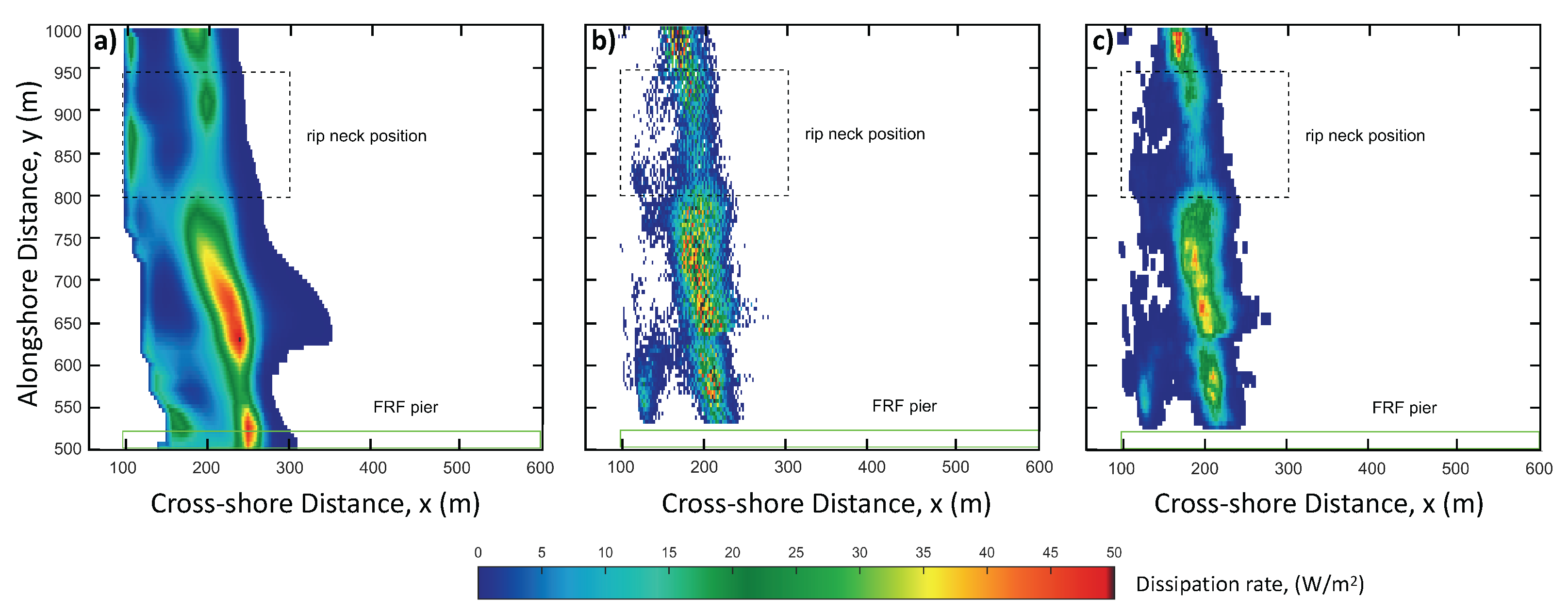
Figure 8a shows a 30 min time exposure of the dissipation rate field, as obtained from the simulation. Most of the dissipation is concentrated over a narrow area, centered about y = 650 m and m and showing a small obliquity. The dissipation rate drops significantly in the alongshore direction, where it can be seen that a dramatic reduction is present near the expected location of a rip observed by Haller et al. [37] (denoted by the dashed box and discussed below). The dissipation rate increases slightly northward of it, but at much smaller magnitudes. Figure 8b shows the corresponding dissipation rate field as obtained from the present method spanning 15 min at the model prediction time. Despite the difference in averaging time between model and data, it is noted that wave conditions did not change significantly during the period, hence the averaged values are directly comparable. The observed dissipation rate field shows some speckle, owing to the discrete sampling of individual events. To minimize this, a spatial averaging is applied, whose result is presented in Figure 8c. While the model shows a larger area of strong dissipation, peak values and overall structure are remarkably similar, despite the possible effect of bathymetry. The observed dissipation rate shows a similar cross-shore extent of breaking, and the alongshore structure is well recovered. Moreover, the location of the maximum dissipation matches well (within 30 m in the cross-shore), and the early onset of dissipation along the m transect is also visible in the observed data. Peak values are within 10%. Considering that no data other than remote sensing and the algorithm presented is used here, the agreement is considered favorable.
The previous result shows the capability of obtaining dissipation rate wave fields. Further, by estimating the dissipation vector, more significant information can be obtained. For example, the rate of change of vorticity can be shown to be proportional to the curl of the dissipation force, in which the dissipation rate is normalized by the local value of , where h is the local depth (e.g., [1,31,49]). In turn, the structure of the vorticity field can be correlated with the location of rip currents (e.g., [1,42]).
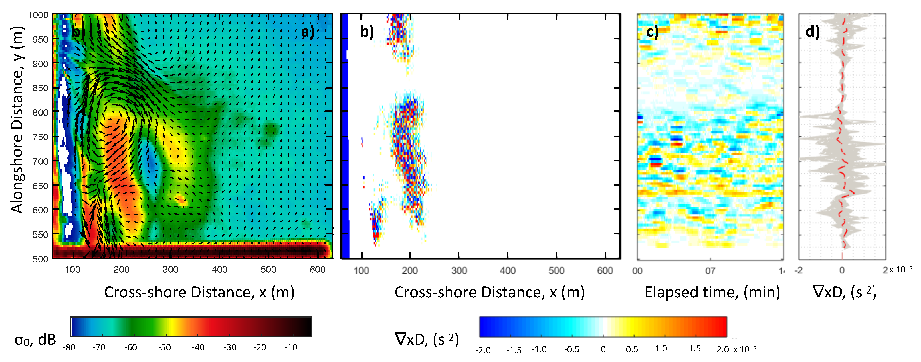
The data collected during R2 allows a qualitative comparison. Haller et al. [37] showed that rip currents were clearly imaged in the marine radar data, and later Wilson et al. [43] were able to use the same model configuration used here to model currents and circulation fields. A sample comparison is shown in Figure 9a where a good correspondence is found. From the dissipation field obtained here, it is possible to estimate the vorticity production . It was assumed that based on the analysis of angles described above.
A 10T average of vorticity production is shown in Figure 9b where, despite significant noise, the presence of a gap is found to be well correlated with the location of the rip neck. Moreover, to the either end of the gap the average vorticity production has opposing signs (thus clockwise and anti-clockwise forcing), which forces the seaward directed currents. Additionally, the time series of data allows analyzing the time series of vorticity production. In Figure 9c,d, the time evolution of an alongshore transect (x = 200 m) is shown. It can be seen that due to the passage of waves, vorticity production can occasionally change direction. However, in the area surrounding the rip neck, vorticity production is relatively stable in time which allows the development of the rip current. This analysis, although qualitative, further highlights the potential of the method.
5.2. Sensitivity Analysis
The methodology presented relies on two potentially-subjective elements. One corresponds to a sensor-dependent threshold, while the other is the value of the free parameter , which controls the dissipation rate. In what follows, we perform a sensitivity analysis for both.
Regarding the threshold selection, it must be noted that this is an element that is closely related to the detection algorithm. In particular this threshold controls the areal extent of the roller as seen by joint video/marine radar procedure. Therefore, it controls the observed length of the roller. Owing to the dependency of the dissipation, this can significantly influence the results. As an example, a comparison changing the video thresholds in R1 and the marine radar in R2 is shown in Figure 10. Only the video thresholds are modified in R1 due to the overcast conditions and large foam production present at that time, which pose a challenge for optical methods [28]. On the other hand, the shorter wave conditions of R2 induce steeper waves that are more difficult to discern from radar data. In Table 3, the test thresholds are listed, where it can be seen that the range of values tested exceeds the expected range of variability for each sensor [28]. In Figure 10 the results of the spatially averaged dissipation fields are shown. Reducing the threshold leads to larger roller lengths and more false detections, hence increased dissipation rates. It also allows for changing the spatial extent of the dissipation, while not significantly changing the underlying spatial structure. This also affects estimation of gradients, which were used to estimating the vorticity production. This highlights the need for a robust detection algorithm—for the present case, it meant visual inspection of the results.
The other key parameter is the roller angle, . In this case, it can be seen that there is a nonlinear dependence () for the dissipation rate. This means that a change between 2 and 20 corresponds to a factor 10 change in the dissipation rate estimate. For the present case, the value 15 was chosen owing to its good agreement with model data. While it can be noticed that this value differs from the used in the model setup, the latter was chosen as a default model parameter and was not subject to experiment-specific calibration. Also, the model assumes the density of water for the roller density (cf. Equation (6)), and this nearly cancels the effect of differing roller angle. Moreover, the value of used in the present methodology is in close agreement with the range of 0.2–0.4 rad (11–22) presented by Zhang et al. [39] for waves in the surfzone after the onset of breaking. In the future, it would be possible to include such parameterizations to further constrain the estimation.
6. Conclusions
A methodology to obtain two dimensional wave breaking dissipation fields in the surfzone has been presented and evaluated. Although in the work presented herein two remote sensors working at different electromagnetic wavelengths are used, in principle the method can be applied to any sensor capable of providing the required geometric parameters of the roller size at sufficient temporal resolution and spatial coverage. This allows tracking roller evolution across the surfzone, which are then coupled with a model for dissipation.
The method allows characterization of the spatial structure of the dissipation field. Although it resembles the structure that is retrieved from time averaging optical images, the method allows determination of the magnitude of the dissipation rate. As a result, other quantities such as the gradient of the dissipation rate, or the dissipation force, can be obtained. These could be used to estimate the forcing of wave related quantities such as currents or mean water levels.
Owing to the lack of direct validation data, results are compared against predicted values from independent modeling using ROMS. The dissipation outputs of model and observations show significant similarities, both in spatial structure and magnitudes, with differences between peak values less than 10%. Moreover, the curl of the dissipation force shows a good correspondence with the presence of rip currents. These results show that the method is capable of providing physically meaningful values of dissipation rates.
Although largely exploratory at this stage, deriving time series of dissipation fields from remote sensing data offers the opportunity to shed more light in the understanding of nearshore hydrodynamics. For instance, wave-by-wave estimates can be averaged at different time scales to further understand the temporal evolution of currents, mean levels and circulation. Other applications consider real-time monitoring, and/or data assimilation in the surf zone. However, more work is required to provide a thorough validation of these results by carrying out a data intensive field campaign.
Acknowledgments
P.A.C. and H.D. would like to thank CONICYT through FONDECYT 1170415, which supported this research and publishing this work. P.A.C. also is funded by CONICYT FONDAP 11550017 and PIA/Basal FB0821.
Author Contributions
Patricio A. Catalan conceived and designed the experiments, collected data, and contributed to the analysis and preparation of the manuscript. Harold Diaz carried out the implementation of the algorithms and data analyses, and contributed to manuscript preparation. Greg W. Wilson carried out the modeling, participated in the analysis and manuscript preparation.
Conflicts of Interest
The authors declare no conflict of interest.
References
- Bonneton, P.; Bruneau, N.; Castelle, B.; Marche, F. Large-scale vorticity generation due to dissipating waves in the surf zone. Discret. Contin. Dyn. Syst. Ser. B 2010, 13, 729–738. [Google Scholar] [CrossRef]
- Longuet-Higgins, M.S.; Stewart, R. Radiation stresses in water waves; a physical discussion with applications. Deep Sea Res. 1964, 11, 529–562. [Google Scholar] [CrossRef]
- Longuet-Higgins, M.S. Longshore currents generated by obliquely incident sea waves: 1. J. Geophys. Res. 1970, 75, 6778–6789. [Google Scholar] [CrossRef]
- Holman, R.; Haller, M.C. Remote Sensing of the Nearshore. Ann. Rev. Mar. Sci. 2013, 5, 95–113. [Google Scholar] [CrossRef] [PubMed]
- Battjes, J.A. Surf-zone dynamics. Ann. Rev. Fluid Mech. 1988, 20, 257–293. [Google Scholar] [CrossRef]
- Battjes, J.A.; Janssen, J.P.F.M. Energy loss and set-up due to breaking random waves. In Proceedings of the 16th Conference on Coastal Engineering, Hamburg, Germany, 27 August–3 September 1978; pp. 68–81. [Google Scholar]
- Le Mehaute, B. On Non-Saturated Breakers and the Wave Run-Up. Available online: https://icce-ojs-tamu.tdl.org/icce/index.php/icce/article/view/2255 (accessed on 26 December 2017).
- Warner, J.C.; Armstrong, B.; He, R.; Zambon, J.B. Development of a Coupled Ocean-Atmosphere-Wave-Sediment Transport (COAWST) Modeling System. Ocean Model. 2010, 35, 230–244. [Google Scholar] [CrossRef]
- Roelvink, D.; Reniers, A.; van Dongeren, A.; van Thiel de Vries, J.; McCall, R.; Lescinski, J. Modelling storm impacts on beaches, dunes and barrier islands. Coast. Eng. 2009, 56, 1133–1152. [Google Scholar] [CrossRef]
- Zijlema, M.; Stelling, G.; Smit, P. SWASH: An operational public domain code for simulating wave fields and rapidly varied flows in coastal waters. Coast. Eng. 2011, 58, 992–1012. [Google Scholar] [CrossRef]
- Shi, F.; Kirby, J.T.; Harris, J.C.; Geiman, J.D.; Grilli, S.T. A high-order adaptive time-stepping TVD solver for Boussinesq modeling of breaking waves and coastal inundation. Ocean Model. 2012, 43–44, 36–51. [Google Scholar] [CrossRef]
- Ma, G.; Shi, F.; Kirby, J.T. Shock-capturing non-hydrostatic model for fully dispersive surface wave processes. Ocean Model. 2012, 43–44, 22–35. [Google Scholar] [CrossRef]
- Duncan, J. An experimental investigation of breaking waves produced by a towed hydrofoil. Proc. R. Soc. Lond. A 1981, 377, 331–348. [Google Scholar] [CrossRef]
- Svendsen, I.A. Mass flux and undertow in the surf zone. Coast. Eng. 1984, 8, 347–365. [Google Scholar] [CrossRef]
- Melville, W.K.; Loewen, M.R.; Felizardo, F.C.; Jessup, A.T.; Buckingham, M.J. Acoustic and microwave signatures of breaking waves. Nature 1988, 336, 54–56. [Google Scholar] [CrossRef]
- Holman, R.; Stanley, J. The history and technical capabilities of Argus. Coast. Eng. 2007, 54, 477–491. [Google Scholar] [CrossRef]
- Catalán, P.A.; Haller, M.C.; Plant, W.J. Microwave Backscattering from Surf Zone Waves. J. Geophys. Res. 2014, 119, 3098–3120. [Google Scholar] [CrossRef]
- Jessup, A.T.; Zappa, C.J.; Loewen, M.R.; Hesany, V. Infrared remote sensing of breaking waves. Nature 1997, 385, 52–55. [Google Scholar] [CrossRef]
- Lehner, S.; Pleskachevsky, A.; Velotto, D.; Jacobsen, S. Meteo-Marine Parameters and Their Variability: Observed by High-Resolution Satellite Radar Images. Oceanography 2013, 26, 80–91. [Google Scholar] [CrossRef] [Green Version]
- Svendsen, I.A. Wave heights and set-up in a surf zone. Coast. Eng. 1984, 8, 303–329. [Google Scholar] [CrossRef]
- Nairn, R.B.; Roelvink, J.; Southgate, H.N. Transition zone with and implications for modelling surfzone hydrodynamics. In Proceedings of the 22nd International Conference on Coastal Engineering, Delft, The Netherlands, 2–6 July 1990; pp. 68–81. [Google Scholar]
- Stive, M.J.; De Vriend, H.J. Shear stresses and mean flow in shoaling and breaking waves. In Proceedings of the 24th International Conference on Coastal Engineering, Kobe, Japan, 23–28 October 1994; pp. 594–608. [Google Scholar]
- Dally, W.R.; Brown, C.A. A modeling investigation of the breaking wave roller with application to cross-shore currents. J. Geophys. Res. 1995, 100, 24873–24883. [Google Scholar] [CrossRef]
- Haller, M.C.; Catalán, P.A. Remote sensing of wave roller lengths in the laboratory. J. Geophys. Res. 2009, 114. [Google Scholar] [CrossRef]
- Díaz Méndez, G.M.; Haller, M.C.; Raubenheimer, B.; Elgar, S.; Honegger, D.A. Radar Remote Sensing Estimates of Waves and Wave Forcing at a Tidal Inlet. J. Atmos. Ocean. Technol. 2015, 32, 842–854. [Google Scholar] [CrossRef]
- Carini, R.J.; Chickadel, C.C.; Jessup, A.T.; Thomson, J. Estimating wave energy dissipation in the surf zone using thermal infrared imagery. J. Geophys. Res. Oceans 2015, 120, 3937–3957. [Google Scholar] [CrossRef]
- Flores, R.P.; Catalán, P.; Haller, M.C. Estimating surfzone wave transformation and wave setup from remote sensing data. Coast. Eng. 2016, 114, 244–252. [Google Scholar] [CrossRef]
- Catalán, P.A.; Haller, M.C.; Holman, R.A.; Plant, W.J. Optical and Microwave Detection of Surf Zone Breaking Waves. IEEE Trans. Geosci. Remote Sens. 2011, 49, 1879–1893. [Google Scholar] [CrossRef]
- Thornton, E.B.; Guza, R.T. Transformation of wave height distribution. J. Geophys. Res. 1983, 88, 5925–5938. [Google Scholar] [CrossRef]
- Thomson, J. Wave Breaking Dissipation Observed with “SWIFT” Drifters. Am. Meteorol. Soc. 2012, 29, 1866–1882. [Google Scholar] [CrossRef]
- Clark, D.B.; Elgar, S.; Raubenheimer, B. Vorticity generation by short-crested wave breaking. Geophys. Res. Lett. 2012, 39. [Google Scholar] [CrossRef]
- Booij, N.; Ris, R.C.; Holthuijsen, L.H. A third-generation wave model for coastal regions 1. Model description and validation. J. Geophys. Res. 1999, 104, 7649–7666. [Google Scholar] [CrossRef]
- Chen, Q.; Kirby, J.T.; Dalrymple, R.A.; Kennedy, A.B.; Chawla, A. Boussinesq modeling of wave transformation, breaking and runup, II:2D. J. Waterw. Port Coast. Ocean Eng. 2000, 126, 48–56. [Google Scholar] [CrossRef]
- Cienfuegos, R.; Barthélemy, E.; Bonneton, P. Wave-Breaking Model for Boussinesq-Type Equations Including Roller Effects in the Mass Conservation Equation. J. Waterw. Port Coast. Ocean Eng. 2010, 136, 10–26. [Google Scholar] [CrossRef]
- Deigaard, R. A note on the three-dimensional shear stress distribution in a surf zone. Coast. Eng. 1993, 20, 157–171. [Google Scholar] [CrossRef]
- Smith, J.A. Wave-current interactions in finite depth. J. Phys. Oceanogr. 2006, 36, 1403–1419. [Google Scholar] [CrossRef]
- Haller, M.C.; Honegger, D.; Catalán, P.A. Rip Current Observations via Marine Radar. J. Waterw. Port Coast. Ocean Eng. 2014, 140, 115–124. [Google Scholar] [CrossRef]
- Buhr Hansen, J. Periodic waves in the surf zone: Analysis of experimental data. Coast. Eng. 1990, 14, 19–41. [Google Scholar] [CrossRef]
- Zhang, C.; Zhang, Q.; Zheng, J.; Demirbilek, Z. Parameterization of nearshore wave front slope. Coast. Eng. 2017, 127, 80–87. [Google Scholar] [CrossRef]
- Reniers, A.; Battjes, J. A laboratory study of longshore currents over barred and non-barred beaches. Coast. Eng. 1997, 30, 1–22. [Google Scholar] [CrossRef]
- Ruessink, B.G.; Miles, J.R.; Feddersen, F.; Guza, R.T.; Elgar, S. Modeling the alongshore current on barred beaches. J. Geophys. Res. 2001, 106, 22451–22463. [Google Scholar] [CrossRef]
- MacMahan, J.H.; Thornton, E.B.; Reniers, A.J. Rip current review. Coast. Eng. 2006, 53, 191–208. [Google Scholar] [CrossRef] [Green Version]
- Wilson, G.W.; Özkan-Haller, H.T.; Holman, R.A.; Haller, M.C.; Honegger, D.A.; Chickadel, C.C. Surf zone bathymetry and circulation predictions via data assimilation of remote sensing observations. J. Geophys. Res. Oceans 2014, 119, 1993–2016. [Google Scholar] [CrossRef]
- Mei, C.C. The Applied Dynamics of Ocean Surface Waves; Wiley: New York, NY, USA, 1983. [Google Scholar]
- Long, C.E. Index and Bulk Parameters for Frequency-Directional Spectra Measured at CERC Field Research Facility, July 1994 to August 1995; Miscellaneous Paper CERC-96-6; U.S. Army Corps of Engineers, Waterways Experiment Station: Vicksburg, MS, USA, 1996. [Google Scholar]
- Svendsen, I.A.; Putrevu, U. Nearshore circulation with 3-D profiles. In Proceedings of the 22nd International Coastal Engineering Conference, Delft, The Netherlands, 2–6 July 1990; pp. 241–254. [Google Scholar]
- Feddersen, F.; Guza, R.T. Observations of nearshore circulation: Alongshore uniformity. J. Geophys. Res. Oceans 2003, 108, 6-1–6-10. [Google Scholar] [CrossRef]
- Smith, S.D. Coefficients for sea surface wind stress, heat flux, and wind profiles as a function of wind speed and temperature. J. Geophys. Res. 1988, 93, 15467–15472. [Google Scholar] [CrossRef]
- Peregrine, D. Surf Zone Currents. Theor. Comput. Fluid Dyn. 1998, 10, 295–309. [Google Scholar] [CrossRef]
Figure 1.
Example of the joint discrimination algorithm. (a) Snapshot of video image; (b) snapshot of marine radar image; (c) snapshot of video image overlain with red, green and cyan dots corresponding to detected active breaking, foam and steepening waves, respectively. (d) pdf of the marine radar data; (e) jpdf; and (f) pdf of video data. Red lines show the thresholds used in this set. In (a–c) waves propagate from the right to the left.
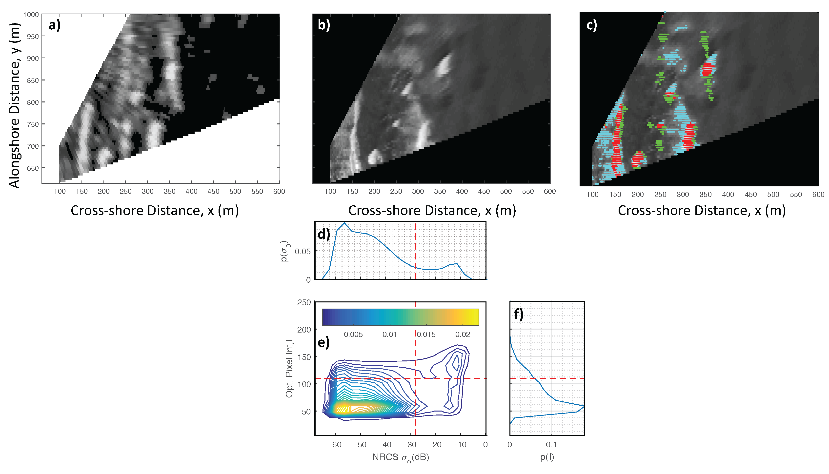
Figure 2.
Definition of relevant geometric variables. (a) Global reference system orientation and propagation angle definition; (b) Example of the centroid tracking among two instances of the same roller. In blue, the displacement of the centroid is presented schematically, along with its components in the global reference system; (c) Local reference system and planform roller parameters. (d) Schematic of the roller geometry and parameters, defined in the local reference system.

Figure 3.
FRF facilities location and coordinate system. FOV denotes the field of view of the cameras, and the solid line is the swath of the marine radar. White dashed lines denote camera boundaries. Black and white image shows the pixel array used.
Figure 3.
FRF facilities location and coordinate system. FOV denotes the field of view of the cameras, and the solid line is the swath of the marine radar. White dashed lines denote camera boundaries. Black and white image shows the pixel array used.
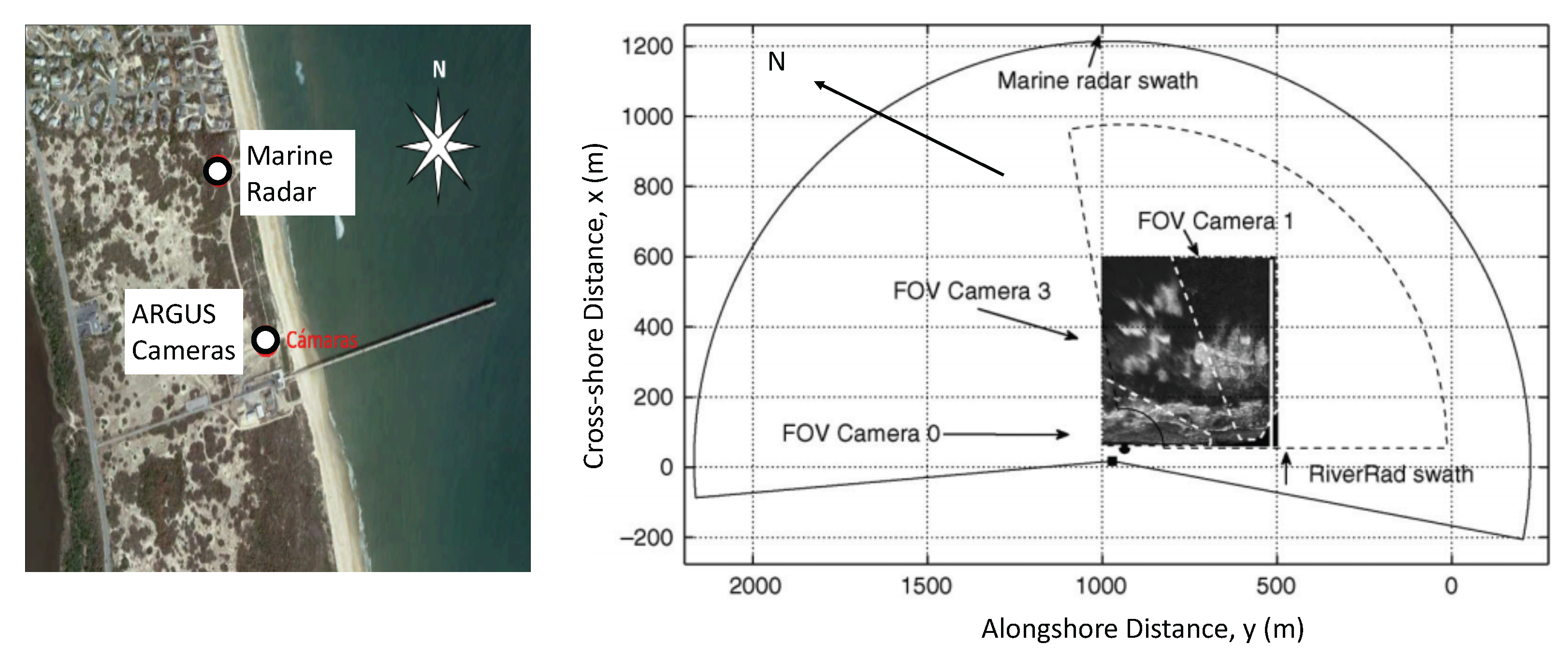
Figure 4.
FOV of each camera for datasets in R1 and R2, (right) and (left) panel respectively. White lines denote camera boundaries, and green boxes denote the sandbar.
Figure 4.
FOV of each camera for datasets in R1 and R2, (right) and (left) panel respectively. White lines denote camera boundaries, and green boxes denote the sandbar.
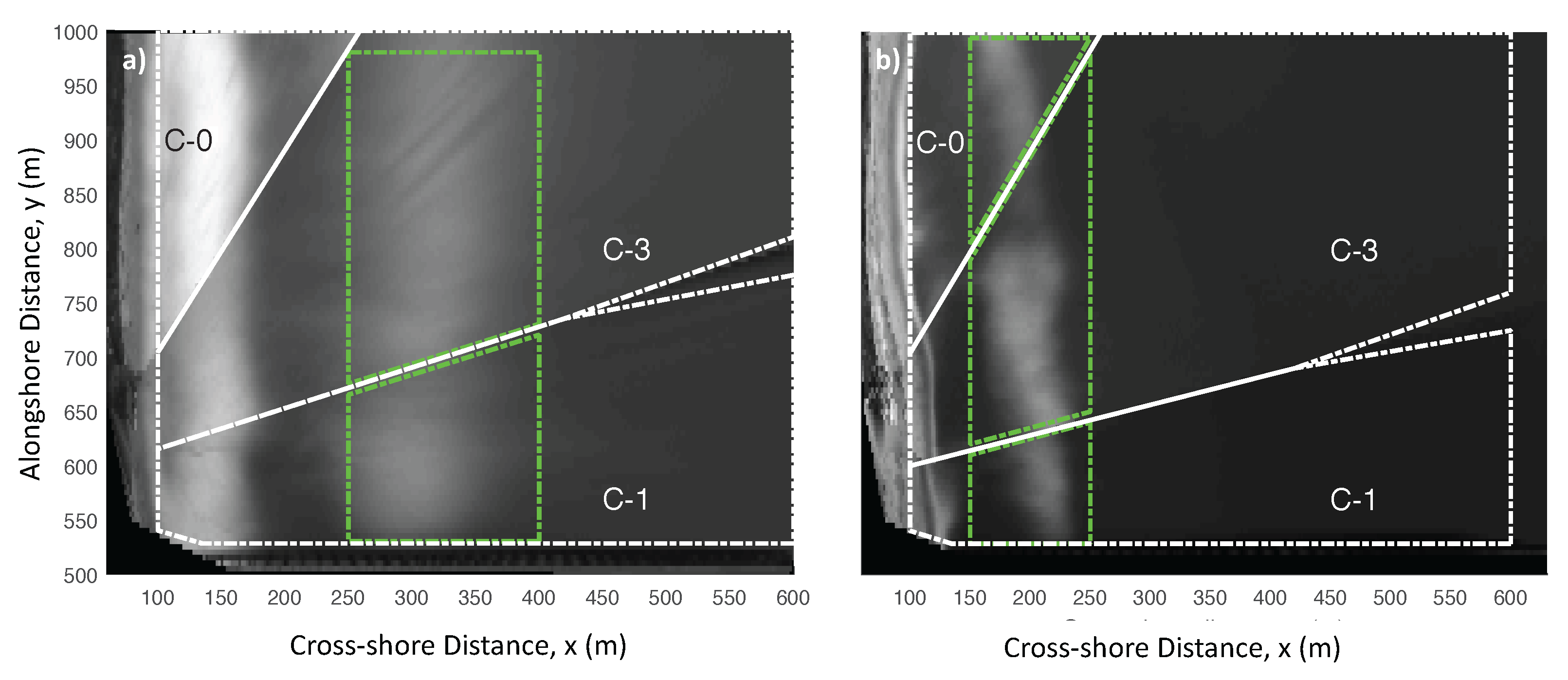
Figure 5.
Example of tracking of a wave roller. (a) Multiple instances of the same roller as it propagates over the surf zone; (b) Time averaged video intensity, where the bright intensity patch corresponds to the roller history shown in a) and whose domain is indicated in the white box; (c) Frame by frame (shades of gray) and net change (green) in position of the roller centroid. Shaded grays denote the same roller identified in consecutive frames.

Figure 6.
Time series of the mean roller length estimated at each frame (thin gray lines). Thick lines correspond to a 10T moving averages, derived from series using (red), (dashed black) and (dashed gray). (a) R1; (b) R2.
Figure 6.
Time series of the mean roller length estimated at each frame (thin gray lines). Thick lines correspond to a 10T moving averages, derived from series using (red), (dashed black) and (dashed gray). (a) R1; (b) R2.

Figure 7.
Wave breaking energy dissipation rate maps averaged over (top) and (bottom). R1 (left) and R2 (right).
Figure 7.
Wave breaking energy dissipation rate maps averaged over (top) and (bottom). R1 (left) and R2 (right).

Figure 8.
(a) ROMS model output of the average dissipation rate, over a 30 min period; (b) Observed average dissipation rate over the entire R2 (15 min); (c) Spatial average of data in panel (b).
Figure 8.
(a) ROMS model output of the average dissipation rate, over a 30 min period; (b) Observed average dissipation rate over the entire R2 (15 min); (c) Spatial average of data in panel (b).

Figure 9.
(a) Time averaged marine radar image from R2 showing the presence of a rip current, overlain velocity vectors obtained by Wilson et al. [43]; (b) Time average (10T) of the curl of the dissipation force; (c) time-space map of the curl of the dissipation force at transect x=200; (d) individual profiles (gray lines) and average (red) of data from panel (c).

Figure 10.
Dissipation rate maps obtained with different thresholds. (Top) row corresponds to results varying (c.f. Table 3) and (bottom) row varying . Threshold values increase from (left) to (right). Note colorscale differs from other figures.
Figure 10.
Dissipation rate maps obtained with different thresholds. (Top) row corresponds to results varying (c.f. Table 3) and (bottom) row varying . Threshold values increase from (left) to (right). Note colorscale differs from other figures.

Table 1.
Summary of wave conditions.
| Dataset | (s) | (m) | MWD (FRF) | Tide (m) |
|---|---|---|---|---|
| R1 | 12.7 | 1.9 | 5 | 0.7 (Mid tide) |
| R2 | 5.8 | 0.7 | −22 | −0.1 (Low tide) |
Table 2.
Video pixel intensity threshold, , non-dimensional.
| Dataset | Cam0 | Cam1 | Cam3 |
|---|---|---|---|
| R1 | - | 85 | 89 |
| R2 | 103 | 80 | 103 |
Table 3.
Summary of thresholds used in sensitivity analysis.
| Dataset | Variable Instrument | Min Value | Mid Value | Max Value | Fixed Instrument | Value |
|---|---|---|---|---|---|---|
| R1 | Camera | 50 | 100 | 150 | Radar | −28 dB |
| R2 | Radar | −50 dB | −28 dB | −15 dB | Camera | 103 |
© 2017 by the authors. Licensee MDPI, Basel, Switzerland. This article is an open access article distributed under the terms and conditions of the Creative Commons Attribution (CC BY) license (http://creativecommons.org/licenses/by/4.0/).
Share and Cite
MDPI and ACS Style
Díaz, H.; Catalán, P.A.; Wilson, G.W. Quantification of Two-Dimensional Wave Breaking Dissipation in the Surf Zone from Remote Sensing Data. Remote Sens. 2018, 10, 38. https://doi.org/10.3390/rs10010038
AMA Style
Díaz H, Catalán PA, Wilson GW. Quantification of Two-Dimensional Wave Breaking Dissipation in the Surf Zone from Remote Sensing Data. Remote Sensing. 2018; 10(1):38. https://doi.org/10.3390/rs10010038
Chicago/Turabian StyleDíaz, Harold, Patricio A. Catalán, and Greg W. Wilson. 2018. "Quantification of Two-Dimensional Wave Breaking Dissipation in the Surf Zone from Remote Sensing Data" Remote Sensing 10, no. 1: 38. https://doi.org/10.3390/rs10010038
Note that from the first issue of 2016, this journal uses article numbers instead of page numbers. See further details here.