Article

Assessing the Performance of a Low-Cost Method for Video-Monitoring the Water Surface and Bed Level in the Swash Zone of Natural Beaches

by
Raimundo Ibaceta
1,*,
Rafael Almar
2,
Patricio A. Catalán
1,3,4,
Chris E. Blenkinsopp
5,
Luis P. Almeida
6 and
Rodrigo Cienfuegos
3,7
1
Departamento de Obras Civiles, Universidad Técnica Federico Santa María, Valparaíso 2390123, Chile
2
IRD-LEGOS, Laboratoire d’Études en Géophysique et Océanographie Spatiales, UMR 5566, CNRS/IRD/UPS, Observatoire Midi-Pyrénées (OMP), Toulouse 31400, France
3
Centro Nacional de Investigación para la Gestión Integrada de Desastres Naturales, CONICYT/FONDAP/1511007, Santiago 7820436, Chile
4
CCTVal-Centro Científico Tecnológico de Valparaíso, Valparaíso 2390123, Chile
5
Research Unit for Water, Environment and Infrastructure Resilience (WEIR), University of Bath, Bath BA2 7AY, UK
6
CNES-LEGOS, Laboratoire d’Études en Géophysique et Océanographie Spatiales, UMR 5566, CNRS/IRD/UPS, Observatoire Midi-Pyrénées (OMP), Toulouse 31400, France
7
Departamento de Ingeniería Hidráulica y Ambiental, Pontificia Universidad Católica de Chile, Santiago 7820436, Chile
*
Author to whom correspondence should be addressed.
Remote Sens. 2018, 10(1), 49; https://doi.org/10.3390/rs10010049
Submission received: 26 October 2017 / Revised: 8 December 2017 / Accepted: 23 December 2017 / Published: 2 January 2018
(This article belongs to the Special Issue Instruments and Methods for Ocean Observation and Monitoring)

Abstract

:
A method to continuously measure bed and water levels along a cross-shore transect of vertical poles is evaluated. This remote sensing based method uses video imagery of swash flows propagating past an array of vertical poles buried on the beach face. Using datasets collected at two beaches in Chile, the method is compared against measurements obtained with conventional co-localized instruments: LiDAR and ultrasonic distance meters. The present video swash pole technique shows good skill in retrieving swash zone bed level and water levels, while providing the possibility to measure morphological variations at time scales varying from wave groups (tens of seconds) to hours. Discrepancies between video and ultrasonic distance meters are found when short time scales are used, for both depositional and erosion events, but longer duration trends are captured well. Water surface elevations at the wave-by-wave scale proved to be accurate for the backwash phase (root-mean-sqaure-error, RMSE down to 0.028 m, R 2 up to 0.89), when compared against LiDAR. However, discrepancies have been found during the uprush phase (RMSE up to 0.062 m, R 2 down to 0.71), when the influence of the pole on the swash flow generates an overestimation of the water surface. Overall, owing to its simplicity of deployment, low cost and reasonable accuracy, the technique is considered suitable for swash studies.

Graphical Abstract

1. Introduction

The swash zone is the nearshore region that defines the transition between land and sea. Incoming bores from the inner surf zone collapse and transform into a thin water lens, leading to a zone of alternately dry and submerged states. The swash zone is highly dynamic, with processes acting at multiple time scales, from the order of seconds (waves) to hours (tides) and days (storms). The majority of research efforts focusing on the swash zone have been devoted to linking time-averaged bulk characteristics of inner surf and swash hydrodynamics with morphological evolution at time scales ranging from hours to days (e.g., [1,2,3]), with less focus on shorter time scales. For instance, individual swash events at the wave-by-wave scale. However, there is consensus in that understanding swash zone processes at these short scales is crucial for understanding the overall morphodynamic response of the swash zone [4].
At short time scales, Hughes et al. [5] and Blenkinsopp et al. [6] showed that morphological changes caused by a single or short series of swash events can be greater than the total morphological change integrated over an entire tidal cycle. Consequently, Puleo et al. [7] suggested that ongoing effort should be made at understanding individual erosion and accretion events. To achieve this, it is essential to properly quantify the shoreface evolution at different scales, starting at the time scale of individual swash event cycles. In this context, swash instrumentation is of critical importance for coastal scientists [8].
Both in situ and remote-sensing approaches are commonly used to measure water surface and bed elevations within the swash zone, using a wide variety of techniques. Holman, R. et al. [9,10] used stacked resistance wires to measure the run up elevation on natural beaches, which allowed a continuous measurement along the beach face. Other researchers have installed pressure sensors at or in the bed to provide local (point) but indirect measurements of water depth [11,12] by typically assuming hydrostatic pressure and linear wave theory [13]. However, the turbulent and dynamic behavior of swash flows may render these underlying assumptions invalid. Nevertheless, dense arrays of buried pressure transducers have been employed to measure the water surface and bed level at the wave-by-wave time scale (e.g., [3]). This technique has been shown to work well at sandy beaches but may return uncertain measurements at gravel beaches. Among other disadvantages of buried pressure transducers is that they can be scoured out by erosive waves, or become clogged by sediments. More recently, improved conductivity-based sensors have been used to obtain the bed level fluctuations even during periods of submerged bed with an accuracy of 1 mm [7,14].
As an alternative to in situ sensors, remote sensing techniques can be used to directly estimate the position of the bed and water level. Ultrasonic Distance Meters (henceforth UDM) use the time-of-flight of sound waves to retrieve the location of either bed or water levels with millimetric accuracy (e.g., [15,16]). They are non-intrusive with either the beach face [16] or fluid flow, but can be affected by the presence of non-desired targets, such as residual foam [17]. Similarly to pressure sensors, they provide only point measurements requiring multiple instruments and complex deployment logistics to increase spatial coverage. In contrast, 2D Laser Scanners (LiDAR) use time-of-flight of laser light to estimate water and bed levels. By using a scanning laser, this instruments enable measurements throughout the swash zone with centimeter accuracy and spatial resolution of O (10 cm), at high sample rates O (20 Hz) [8,18,19,20,21,22]. However, LiDAR requires the presence of a turbulent and aerated water surface to scatter the incident beam. Thus erroneous measurements can be obtained for non-saturated waves with a non-aerated water surface, for instance, during the backwash phase. LiDAR can also be more sensitive to problems with the stability of the supporting platform, where standard deviations on bed levels of up to 4.2 (mm) have been reported by Vousdoukas et al. [18].
Remote sensing methods based on images within the optical range of electromagnetic wavelengths have been widely used to study nearshore processes. They offer the potential to extract diverse information at a wide range of frequencies over large spatial domains. Optical methods can be used to measure the variations of the bed or the water levels by contrasting their signal against a known reference, thereby allowing the interface to be tracked. For example, such methods have been used in the swash zone to track the run-up motion, the edge of which is determined by algorithms based on color contrast between water and sand (e.g., [9,23,24]) and recently [25], or inserted poles (see below for details). Other methods rely on stereo-metric intersection—for instance, to map the shoreface elevation, thus allowing morphology mapping with a vertical accuracy of 1 cm (e.g., [26,27]). Similar techniques used under laboratory conditions yield more accurate and dense morphological measurements in-between individual swash events (e.g., [28,29]), although Chardón-Maldonado et al. [30] comment that it is not clear if this technique can be used in the field owing to the highly accurate instrument set up required.
A limited number of previous studies have attempted to use video images of in situ poles to obtain wave measurements in the field. Mizuguchi [31] measured water surface elevations in the swash zone by photographing poles inserted into the beach face at 0.2 Hz, but did not study bed level variations in detail. The DUCK85 [32] and SUPERDUCK [33] experiments used vertical poles, visually aligned by an observer on-shore, to measure the water level in the surf zone at 5 Hz, assuming that each pole remained aligned in the vertical direction.
Partially buried poles have also been employed to measure morphological changes across the beach face. Weir et al. [34] measured the bed elevation against a set of poles every 15 min with a spatial spacing of 2 m, during almost a tidal cycle, claiming an accuracy of 1 cm. Larson et al. [35] used an array of iron poles on a modified beach to measure the beach profile change with a spatial spacing of 0.5 m. They used video cameras to register the bed level every minute with a vertical resolution of 1 mm, but they did not account for the local influence of the poles on the bed, nor the effect of incident waves on the deployment or stability of the poles. Similar set-ups have been used (e.g., [36,37,38,39]) with a 1 cm estimated accuracy and sampling rates varying from 10 s up to 15 min and more. While these methods have been used by a range of authors, a quantitative assessment of their performance has not been carried out to date.
Considering the importance of the swash zone in controlling beach face morphology, and the cost and difficult logistics involved in deploying conventional instruments, a simple and inexpensive pole technique that derives the water surface and bed levels through a semi-automated analysis of optical imagery is valuable. The accuracy of the method is compared against established methods (LiDAR and UDMs), with the objective of assessing the performance and capabilities of this approach. Advantages and drawbacks are discussed considering different time scales (wave-by-wave to hourly evolution). Finally, concluding remarks and guidelines for the use of this technique are provided.

2. Materials and Methods

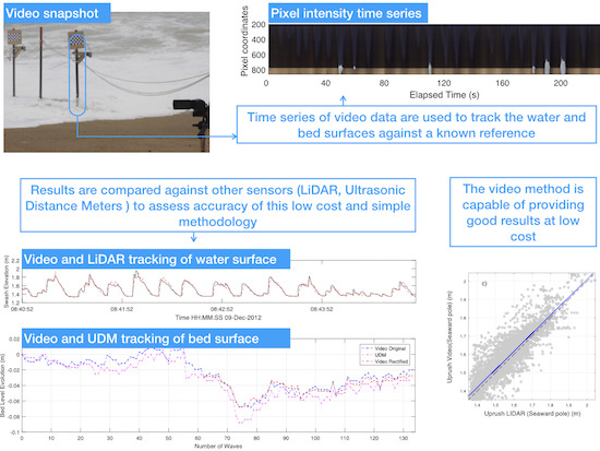
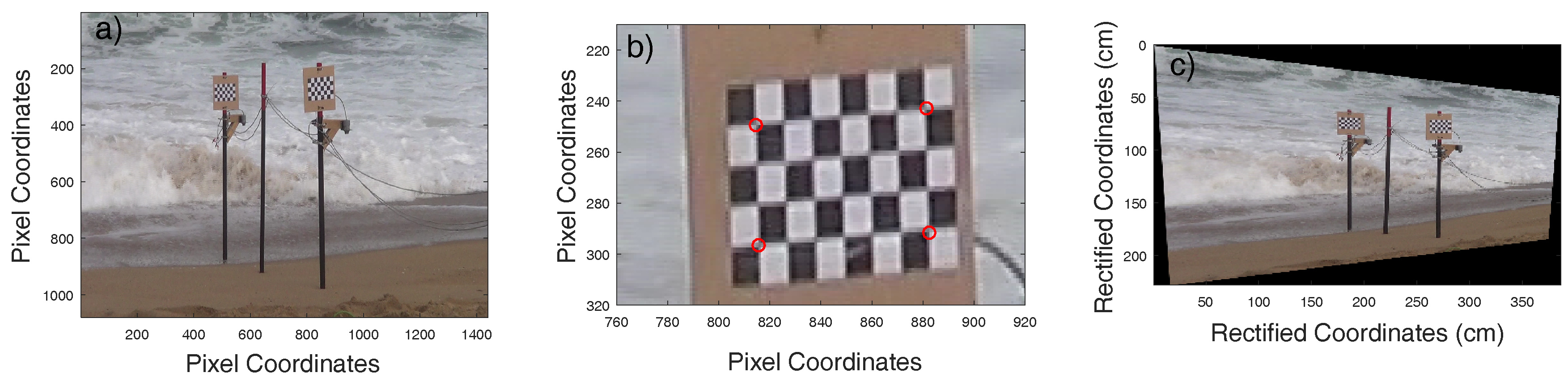
2.1. Experimental Set Up

The experimental setup consists simply of establishing an array of partially buried metallic poles in the swash zone. Data collection is undertaken using video of the entire cross-shore transect using an off-the-shelf, high definition camera mounted on a tripod. For the experiments reported here, a SONY HDR-CX190 FULL HD (∼US$250) video camera (1-7-1 Konan, Minato-ku, Tokyo, Japan) with an acquisition rate of 30 Hz was used. This allows for an inexpensive setup with minimal requirements.
While the spatial arrangement tested here uses poles deployed a cross-shore transect, other arrangements can be used provided they do not obstruct each other within the camera field of view. A small diameter (∼3 cm) is required to reduce the influence of the pole on the hydrodynamics and minimise scouring while providing an identifiable surface to contrast against. The poles are buried vertically approximately 1 m below the initial bed level to ensure stability during acquisition. The poles protrude about 1.5 m above the bed.

2.2. Field Data

The technique was tested during two field experiments conducted in Chile, at Mataquito and Reñaca beaches, and the performance was compared against two other established techniques (LiDAR and UDM). The method was deployed for the first time in Mataquito ( 34 52 S, 72 09 W), nearly 300 km southwest of Santiago de Chile. The beach is dissipative to intermediate, with an alongshore average slope of 0.05 in the intertidal zone, as obtained from beach surveys by Cienfuegos et al. [40]. Data from 9 December 2012 are used here, when incident wave conditions (significant wave height H s = 1.4 m, peak period T p = 9.4 s) were measured using a Teledyne ADCP (1049 Camino Dos Rios, Thousand Oaks, CA, USA) moored at 8 m water depth. An industrial LiDAR (SICK LMS511-10100, Waldkirch, Germany) was deployed at the top of a scaffold, 7.3 m above the beach (Figure 1a) to provide measurements of the bed/water surface elevation along a single transect through the swash and inner surf zone at 35 Hz. A single cross-shore transect of six yellow painted poles with a spacing of 5 m was deployed at an offset of 3 m in the alongshore direction from the LiDAR cross-shore transect (Figure 1b). During the experiment, it was found that some of the poles were insufficiently buried. This led to vibration and tilting of the exposed part of these poles with respect to their original vertical position. Therefore, only a 30 min time series from two cross-shore locations were deemed usable (Figure 1e, Landward Pole and Seaward Pole). The vertical elevation and position of each pole was measured with GPS at the beginning of the deployment, in order to reference the video series relative to LiDAR measurements using a common datum.
A second experiment was conducted in September 2015 at Reñaca Beach, Viña del Mar, Chile ( 32 58 S, 71 32 W), nearly 120 km west from Santiago. Unlike Mataquito, Reñaca is a steep, reflective beach, providing contrasting conditions for testing the photo pole method. Incident wave conditions during this field study were obtained from hindcast data due to malfunctioning of a moored ADCP. Wave conditions of H s = 1.31 m, T p = 11.17 s were retrieved from a node of the Chilean database located offshore of Reñaca [41]. An alongshore uniform swash slope of 0.1 was obtained from beach surveys undertaken during the experiment. To avoid the pole instability problems observed at Mataquito, the poles at Renãca were buried to a greater depth. Three poles were deployed on a cross-shore transect at 2 m spacing (Figure 1c,f). Two ultrasonic distance meters (MASSA M300-95, 280 Lincoln Street, Hingham, MA, USA, Figure 1d) were co-located with the landward and seaward poles at vertical distances of 0.8 m and 1.1 m from the initial bed level, respectively. Ultrasonic and sampling frequencies were configured to be 95 kHz and 4 Hz, respectively, with sub-millimeter vertical resolution. The alongshore distance between poles and the center of the ultrasonic beam was 0.19 m. At least 60 min of synchronized measurements are available for validation at both positions. Unfortunately, foggy conditions characterized the daylight hours of the Reñaca during the field experiment. The presence of fog reduces the image contrast required for accurate determination of the foamy water surface. Therefore, the analysis of this dataset focuses on the bed elevation validation only.

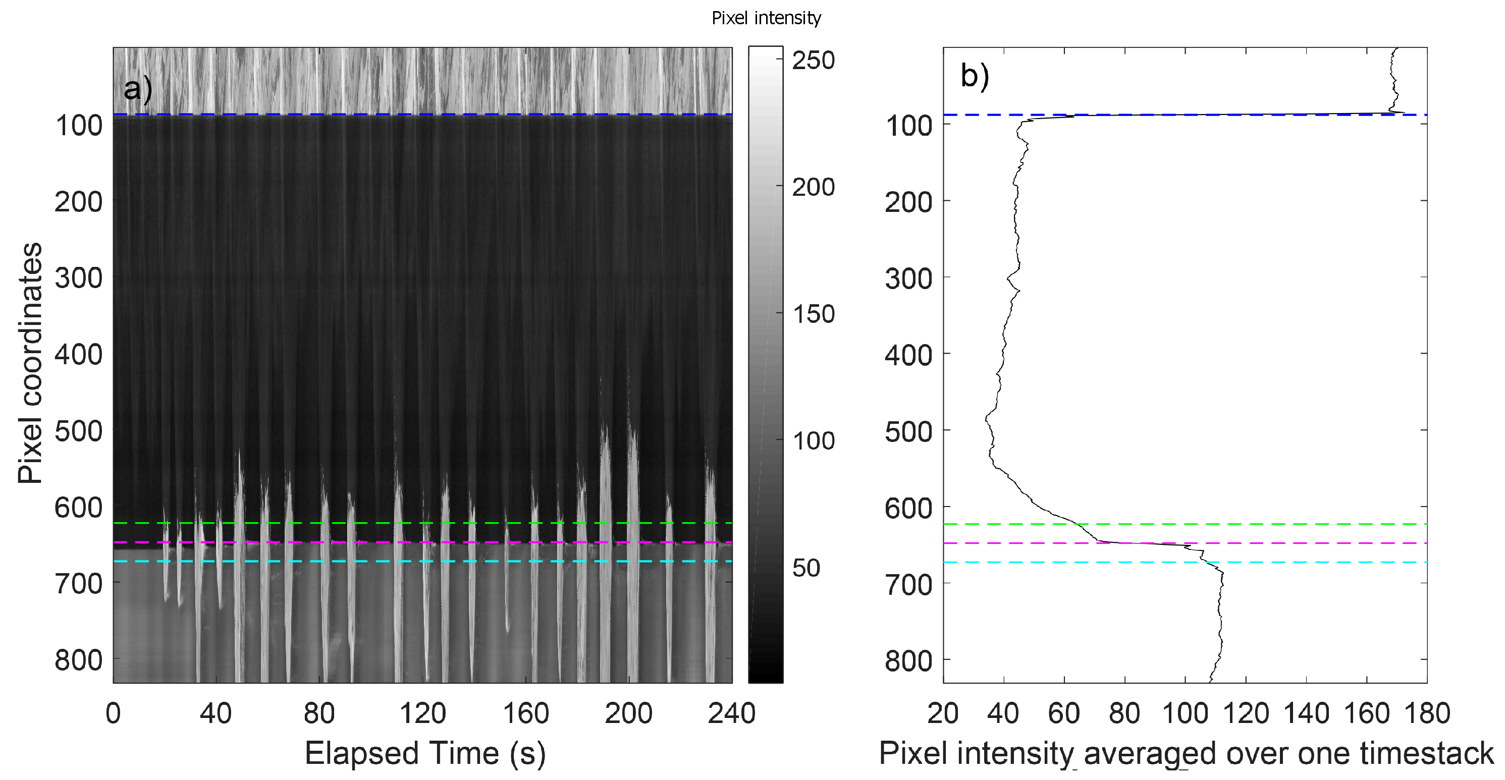
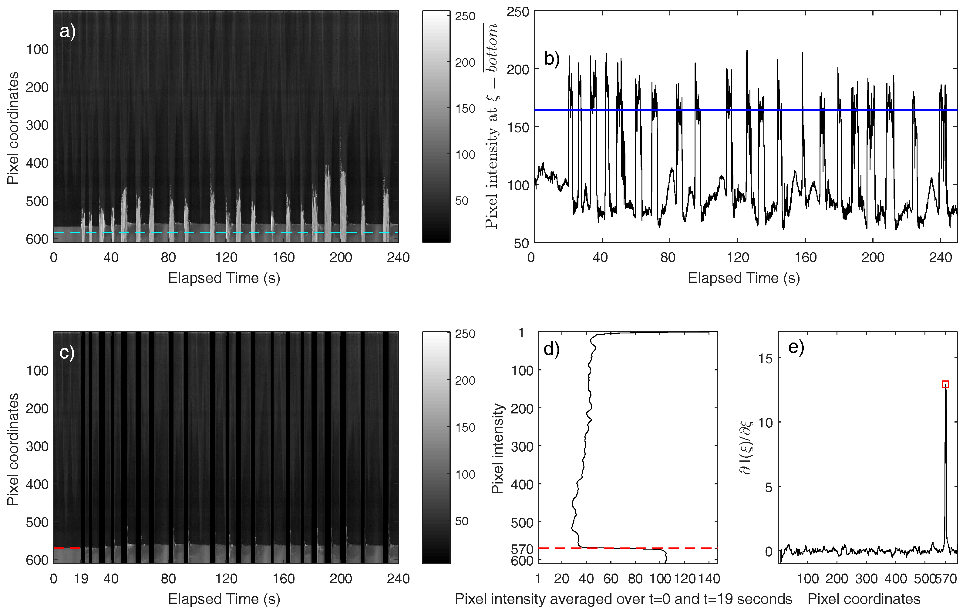
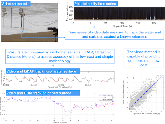
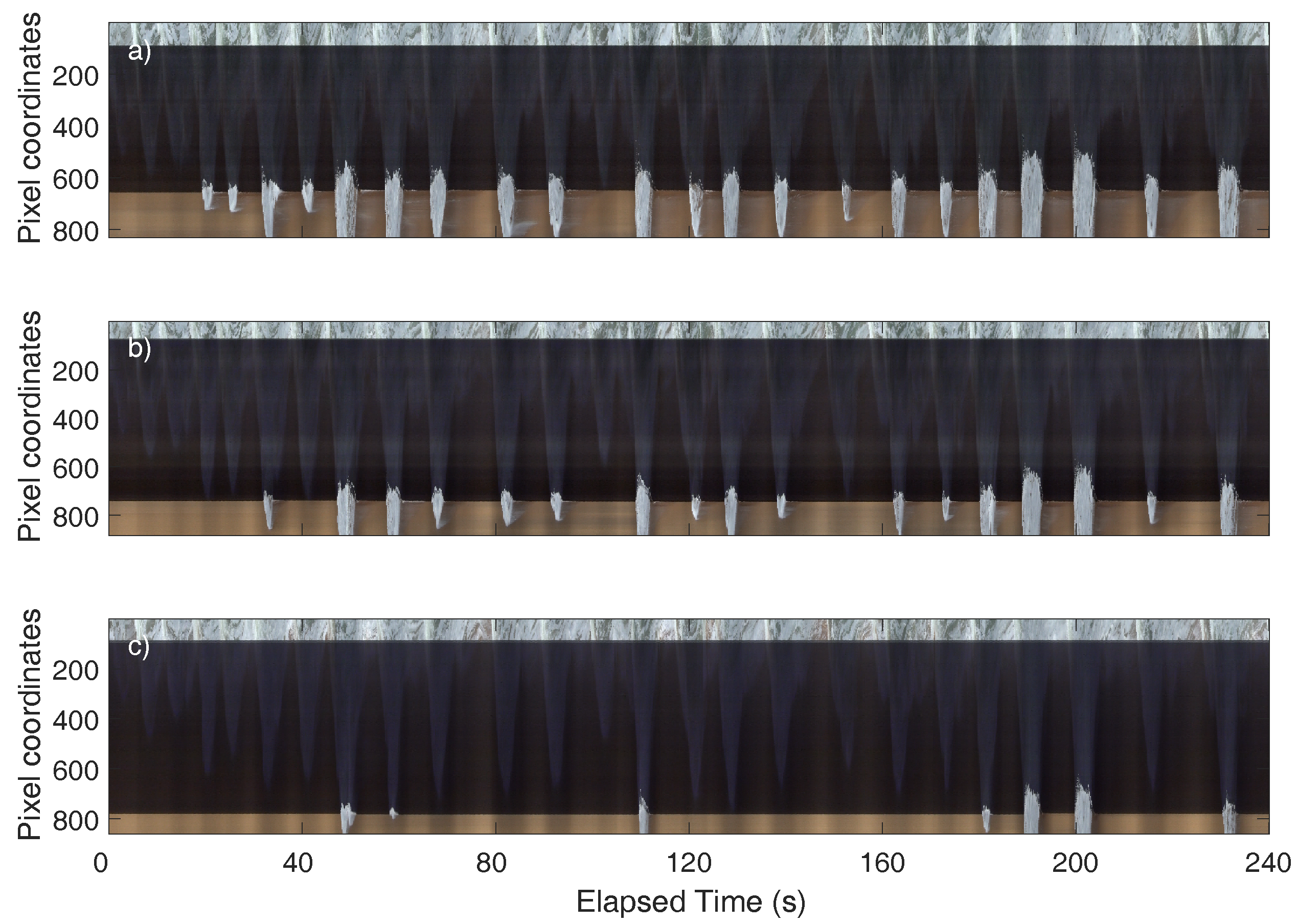
2.3. Image Processing

The rationale of the method is to extract the instantaneous location of a surface use by continuously tracking the interface between the surface and the pole. By having several poles within the field of view, synchronization is ensured, but the trade-off is that pixel resolution decreases as distance from the camera increases.
Each pole is analyzed independently of the others. To reduce data to a single pole, Hovmoller diagrams (henceforth termed time-space images) of optical intensities are stored by color channel (RGB, Red, Green, Blue). The time-space images are generated by extracting an array of pixels from each video frame along the pole axis and concatenating them in time. The duration of these images can be freely adjusted and it is assumed that the pole does not move enough to alter the mapping of a given pixel to the corresponding point in the pole. Here, durations of 2 to 4 min are used to focus on individual event swash dynamics. To illustrate, Figure 2 shows 4-min time-space images at three cross-shore positions. Incident bores from the lower swash zone (top panel, white and light color features) progress toward the upper part of the beach, while decaying in size and lifespan. Only a few bores reach this position (bottom panel). The pole–sand interface is easily identifiable.

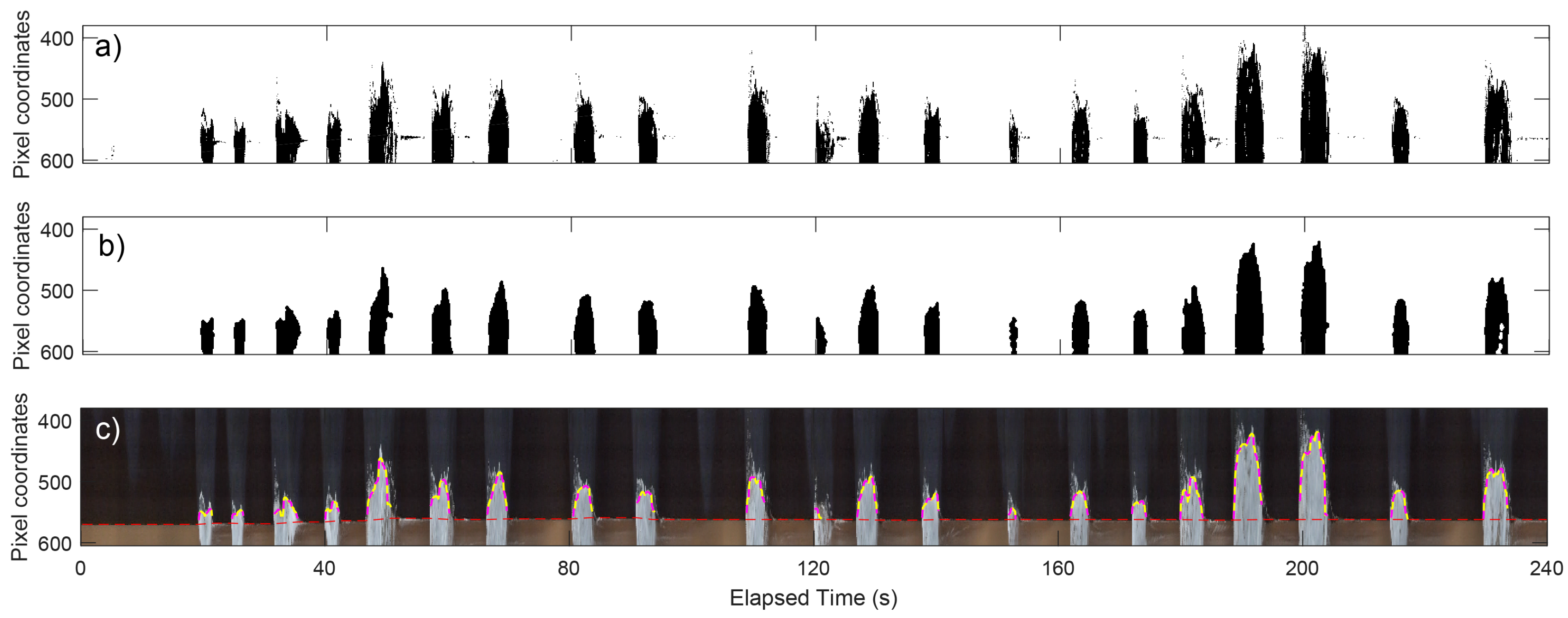
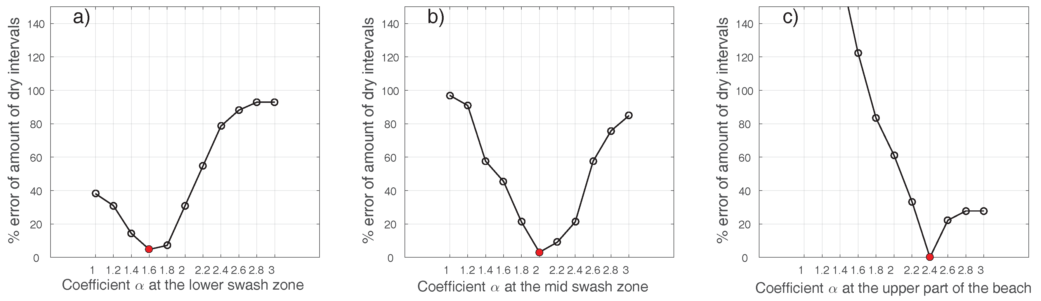
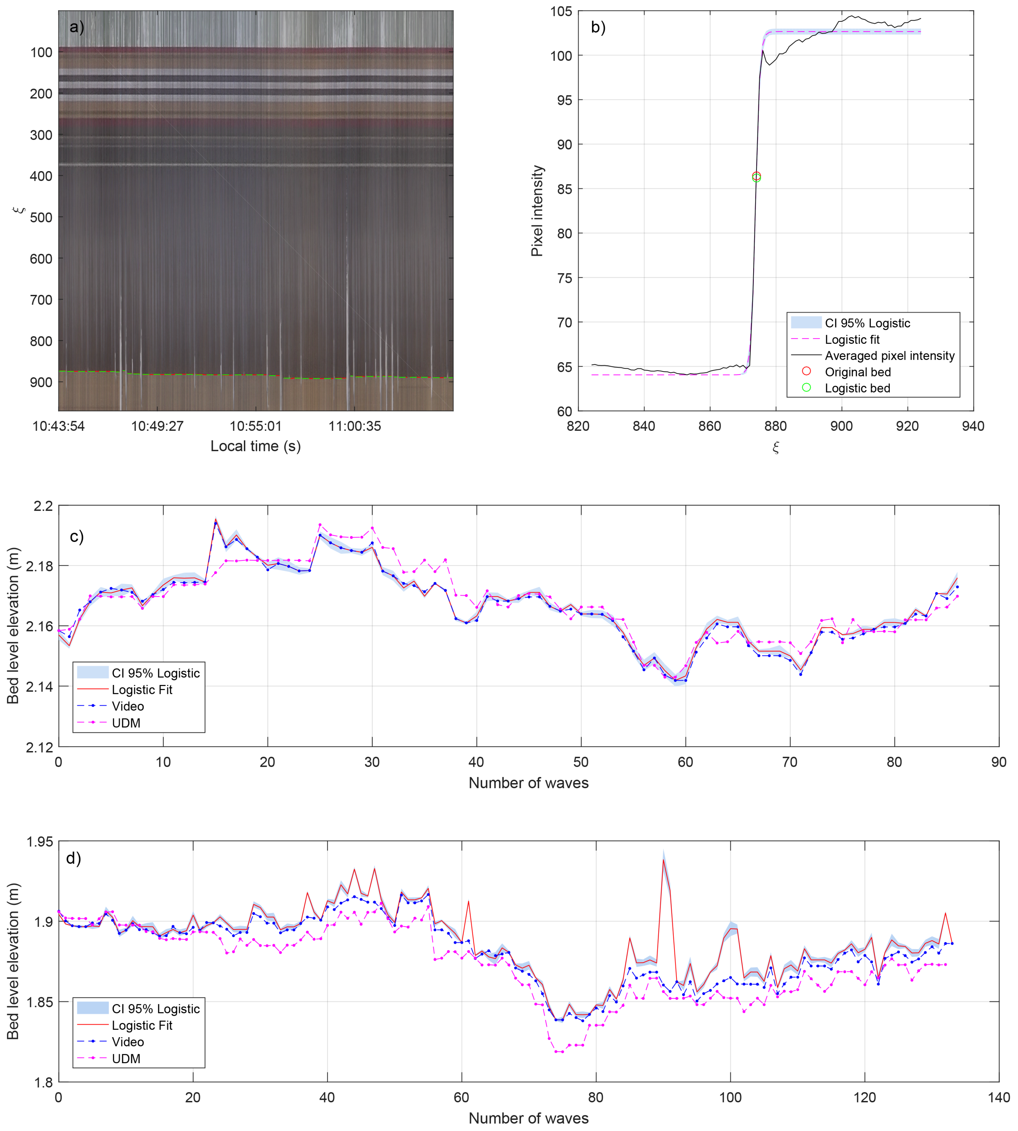
2.4. Bed Level and Water Surface Detection

Bed and water surface levels are computed separately, but following the same approach. The basic assumption is that the bed level can be observed when water is absent, and that the water level can be observed when the pole is partially submerged during each swash event. In what follows, a swash event is defined as the interval between consecutive dry bed occurrences, following Blenkinsopp et al. [6]. Therefore, it is necessary to separate dry and wet periods to identify the bed or water surface, respectively. While the procedure is conceptually the same, it involves the analysis of different sections of the image. Distinguishable color contrast between the pole and the water surface (or bed level) allows for the identification of the instantaneous location of the interface. By noting the strong contrast between the black color of the pole with the light or white colors of the, typically foamy, water surface; and the color of the sand, a simple thresholding procedure can be used used. Once the interface is identified in pixel space, it is transformed to real world coordinates.
RGB time-space images are first converted to intensity gray scale images, defined as I ( ξ , t ) , where ξ is the vertical coordinate (in pixels) along each pole; and t is the time index coordinate (in frames). Next, the time-space image is averaged in time to yield a time-averaged pixel intensity profile, which is used to identify areas of interest for the subsequent analysis. An example is shown in Figure 3, where a clear change in pixel intensity is observed between the pole and the area of interest. The middle section of the time-space image corresponds to the pole and is characterized by relatively constant low pixel intensity value, which fluctuates little due to changes in lightning conditions. The average pixel intensity I ¯ ( ξ ) increases gradually when the pole is partially immersed by swash flow ( ξ = 500 650 ), followed by a sharp increase in pixel intensity at the sand level (magenta line). Note that the pixel coordinate increases towards the bottom of the pole.
The use of the time-averaged pixel intensity profile allows the identification of reference features in the image. The mean bed level, herein termed b e d ¯ ( shown in magenta in Figure 3b), is defined as the ξ coordinate that is detected by the abrupt change in optical intensity described above. Considering that bed changes should be confined around this mean level, an area of interest for bed tracking is bounded at the bottom of the time-space image by arbitrarily defining a location n y pixels below ξ = b e d ¯ , where n y is a fixed value defined by the user. Here, n y is set to 50 pixels, which in this case corresponds to 5–20 cm depending on distance of the pole to the camera. To identify the bed level, a new vertical location in the image is selected and termed b o t t o m ¯ (c.f. Figure 3, cyan dashed line), by selecting a time series 0.5 n y pixels below the mean bed level. The pixel intensity time series at this location shows alternating periods of large and low pixel intensity, with sudden and sharp gradients in between. The periods of large intensity are expected to be due to water covering the pole and bed. Thus, a simple thresholding procedure can be used to discriminate these events. The threshold intensity I t h r B is defined as:
I t h r B = I ¯ ( b o t t o m ¯ ) + α σ ( I ( b o t t o m ¯ , t ) ) ,
where α is a coefficient that varies depending on site and the cross-shore position, and σ is the pixel intensity standard deviation of the time series. Figure 4 shows the application of I t h r B to a series collected at the lower swash zone at Renãca (Figure 2a), where swash events are relatively long in duration. Optical pixel intensity along ξ = b o t t o m ¯ (Figure 4b) has values between I 70–120, defining moments without water. These intervals are interrupted by high intensity values ( I > 150 ) associated with foamy swash events. The solid blue line indicates a threshold intensity of I t h r B = 164.4 , estimated using Equation (1), with α = 1.6 . Continuous pixel intensities above the threshold, I > I t h r B , are considered to be part of a single swash event.
Using this approach, I ( ξ , t ) is transformed into a matrix with identified intervals of bed level and swash events (Figure 4c). To minimize false detection due to splashing, a duration criterion is imposed assuming that swash events must last more than one 1 s.
Once swash events have been filtered out, the bed level is determined at each time interval by computing the gradient in pixel intensity along the pole axis, I ¯ ( ξ ) ξ . Due to color changes, the maximum gradient corresponds to the transition between the pole and the sand, thereby denoting the location of the bed level. Figure 4c,d,e show sample results over a 19 s window. The procedure detailed above is applied to each interval between swash events to determine the changing bed elevation on a swash-by-swash basis.
A similar procedure is applied to identify water surface but with a modified threshold:
I t h r W = I ¯ ( o v e r b e d ¯ ) + β σ ( I ( o v e r b e d ¯ , t ) ) ,
where β defines the number of standard deviations above the mean of I ¯ ( o v e r b e d ¯ , t ) and o v e r b e d ¯ is a level, which is offset 0.5 n y above the mean bed level (Figure 3a, green dashed line). Due to potential splashing on the pole, an erosion–dilation morphological image filter is applied to reduce the effect of droplets or small scale features on the record.
Following the thresholding technique described above, I ( ξ , t ) is transformed into a binary map of ones (water pixels) and zeros (pole or bed pixels), as shown in Figure 5a. Figure 5b shows the binary matrix after application of the erosion–dilation filter, which successfully removes noise present in the signal due to splashing and foam, and allows for simple determination of the interface without affecting the main structure of the swash event.
A transformation from pixel to real world coordinates is conducted by assuming a weak lens distortion, and that the pole belongs to a vertical plane parallel to the image plane. The validity of these assumptions is reviewed below. Hence, any known dimension of the pole can be used to estimate the pixel resolution and transform to world coordinates. Here, a 30 cm painted section in the upper section of the pole is used to estimate the pixel resolution. Typical resolutions (pixel footprint) of O ( 10 3 m/pixel) are obtained, decreasing with the distance to the camera. Table 1 shows the pixel resolutions obtained in the present study. Vertical levels are then geo-referenced to a common datum by referring to the position of the top of the pole, which was measured using RTK GPS.

3. Results

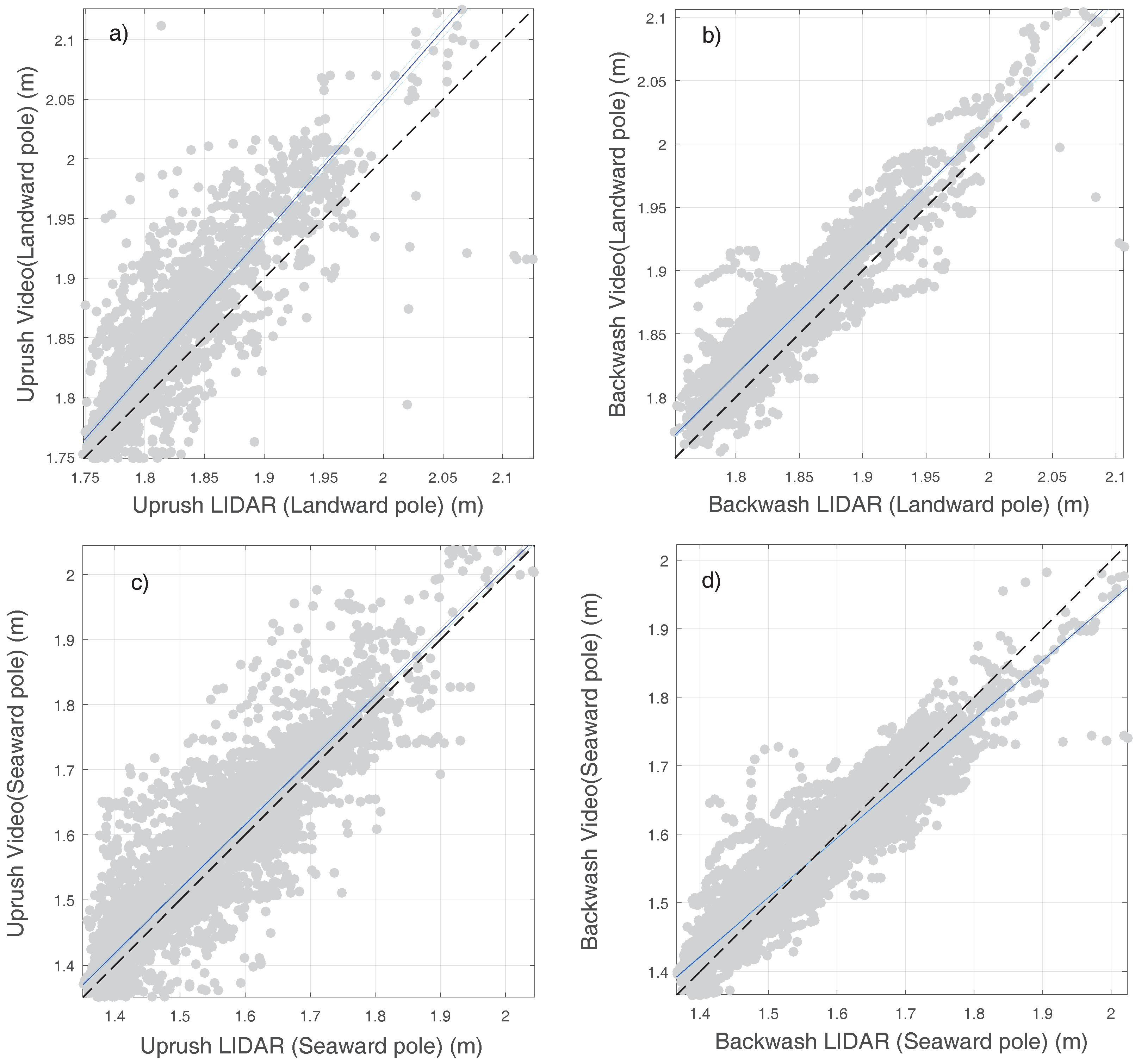
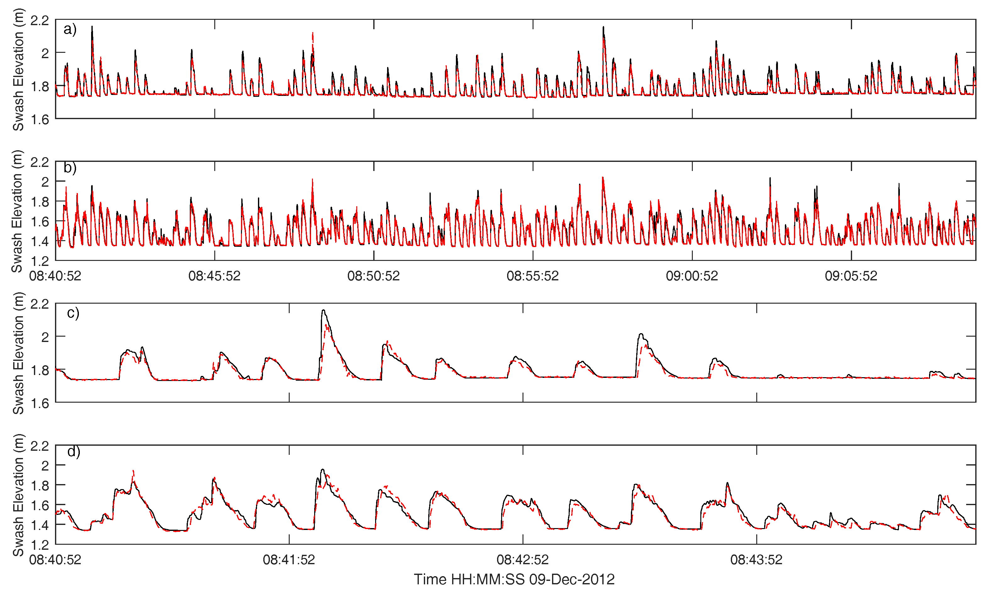
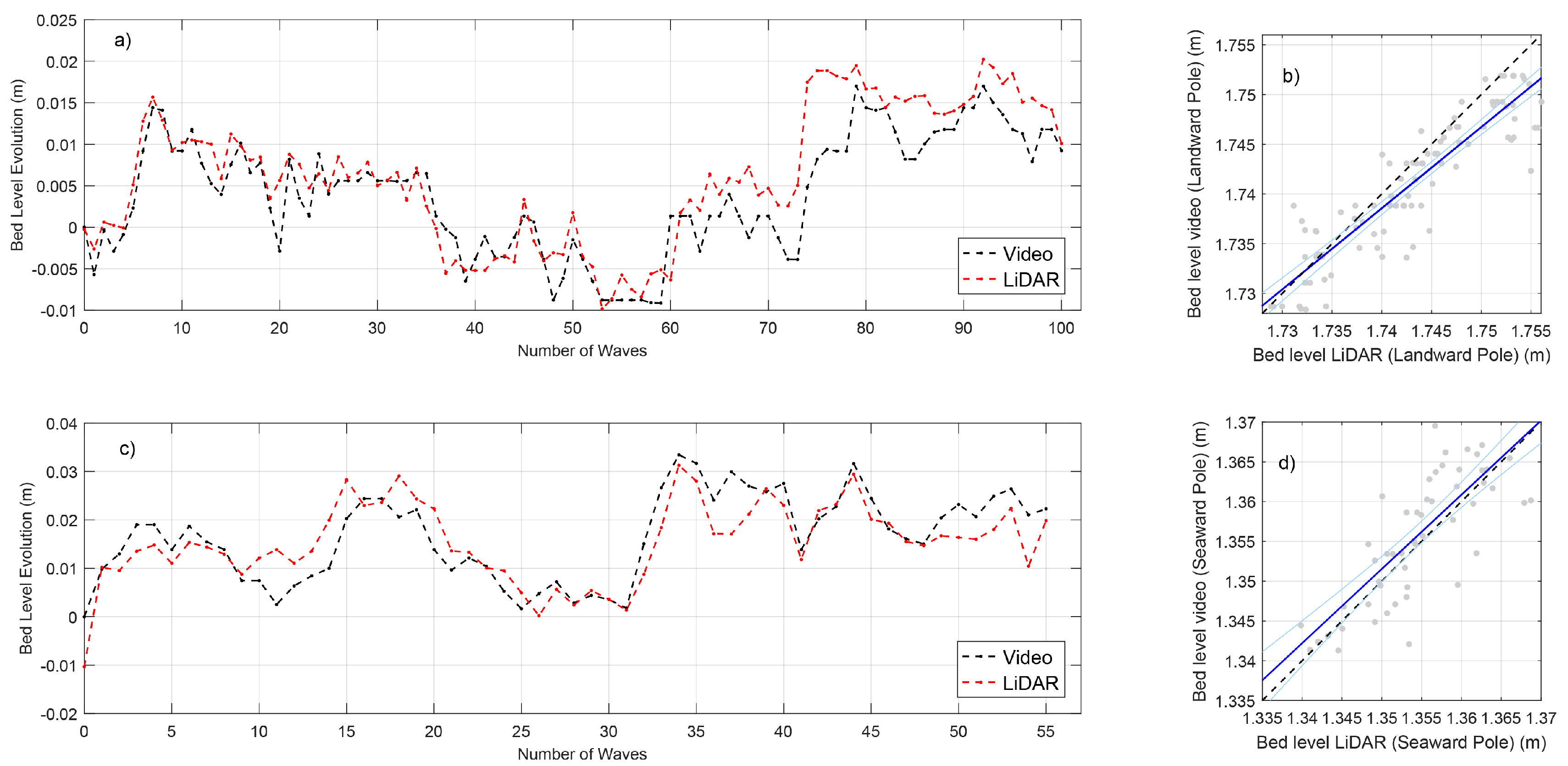
3.1. Comparison with LiDAR for the Water Surface and Bed Level

Raw LiDAR measurements were de-spiked to reduce outliers, and random noise was reduced using a filter with a moving time-average with a window of 0.2 s (e.g., [20]). LiDAR data were down-sampled to match the video frame rate. Bed and water levels were separated using a variance threshold Almeida et al. [19] at each pole location, and extracted using a threshold water depth of 0.02 m to distinguish from topography.
Figure 6a,b show 30 min time series of LiDAR (red dashed line) and video (black solid line) for both the landward and seaward pole locations. An overall excellent agreement is observed, with root-mean-square-error (RMSE) differences of 0.023 m and 0.044 m, respectively (see Table 2 for a summary of statistics). Figure 6c,d show 5 min detail from both cross-shore positions. Errors arise primarily around the time of swash front arrival, when the pole method has a tendency to overestimate the water level.
A comparison of the two techniques for the uprush and backwash phases separately can be observed in the scatter plots presented in Figure 7. In these plots, the best fit regression using a linear model η Video = a η LiDAR + b are also presented, where η is the water level. Regressions computed with the 95% confidence regression values are shown in cyan. For these cases, they are very similar to best fit regression, indicating a large confidence in the estimates of the latter.
Uprush–backwash separation was computed by identifying the turning point between increasing (uprush) and decreasing (backwash) values of a low-pass filtered water surface signal (frequency cut-off 0.5 s 1 ). This is considered appropriate for the bulk analysis here, although flow reversal might actually occur before this criterion. Uprush measurements at both poles exhibits a good correlation between LiDAR and video data, with a minimum R 2 = 0.71 . The present method has a tendency to overpredict the elevation, particularly at the landward pole, which has a slope fit term exceeding unity. Backwash phases show an improved correlation, with maximum R 2 up to 0.89 . Better correlations and less scatter are found for backwash than uprush phases.
Analysis of the bed elevations extracted from the photo poles indicates that the overall trend in bed elevation changes are captured well at both pole locations (Figure 8a,c). Differences in the absolute bed level elevations are comparable, with maximum differences of 1.2 cm between video and LiDAR. On a swash-by-swash basis, the correlation between the LiDAR and photo pole data is R 2 = 0.82 (RMSE = 0.004 m) and R 2 = 0.69 (RMSE = 0.005 m) for the landward and seaward poles, respectively (Figure 8b,d). These regression parameters are comparable to those obtained for the water surface elevation.
With the aim of further demonstrating the capability of video for measuring the absolute bed level, the relative difference between common intervals of bed level, defined as
E = z i , LiDAR ¯ z i , video ,
were calculated, where z i , LiDAR ¯ is the mean value of the LiDAR time series during the ith bed level interval and z i , video , the corresponding bed level retrieved by video. Furthermore, 101 and 56 intervals of common bed level exposures were found at the landward and seaward pole, respectively. A large fraction of them, 82% and 71%, yield E < 5 mm, which is within the expected accuracy of LiDAR.
The cumulative bed level change relative to the number of waves (swash events) is shown in Figure 8a for the landward pole, where 100 waves were identified. Both LiDAR and video yield very similar trends with an overall consistency between erosion and deposition cycles. However, individual swash events can vary significantly and show opposite behavior on occasion. This is likely to be due to low resolution of video relative to the magnitude of bed level variations at the wave-by-wave scale and the 3 m alongshore separation between both measurements. Similar trends are found for the seaward position (Figure 8c, 55 waves).

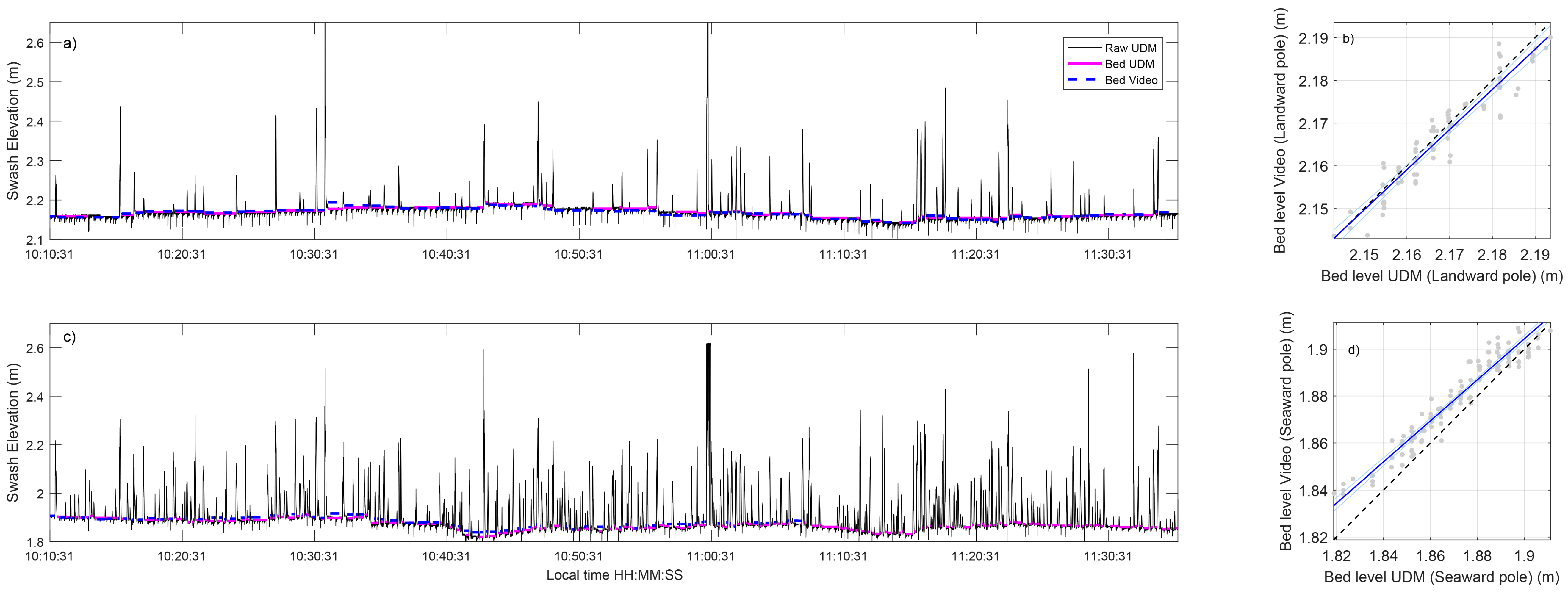
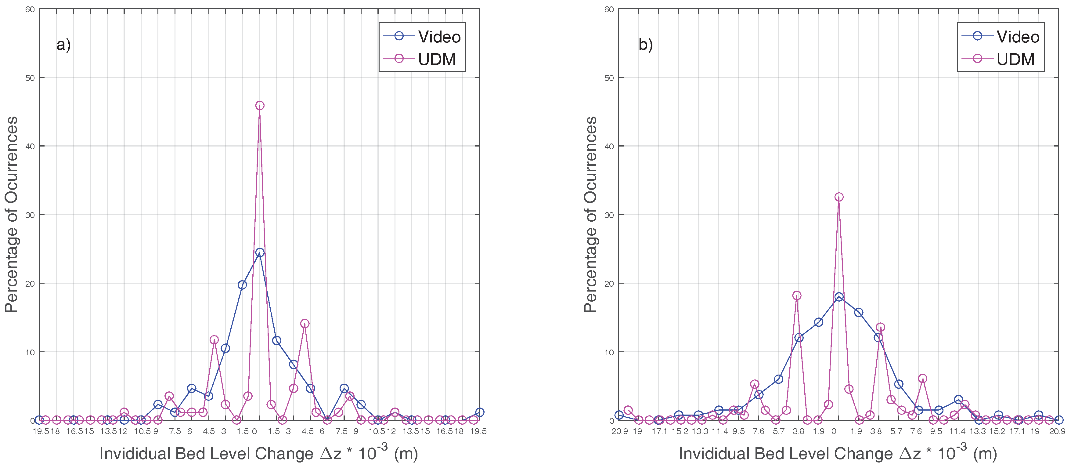
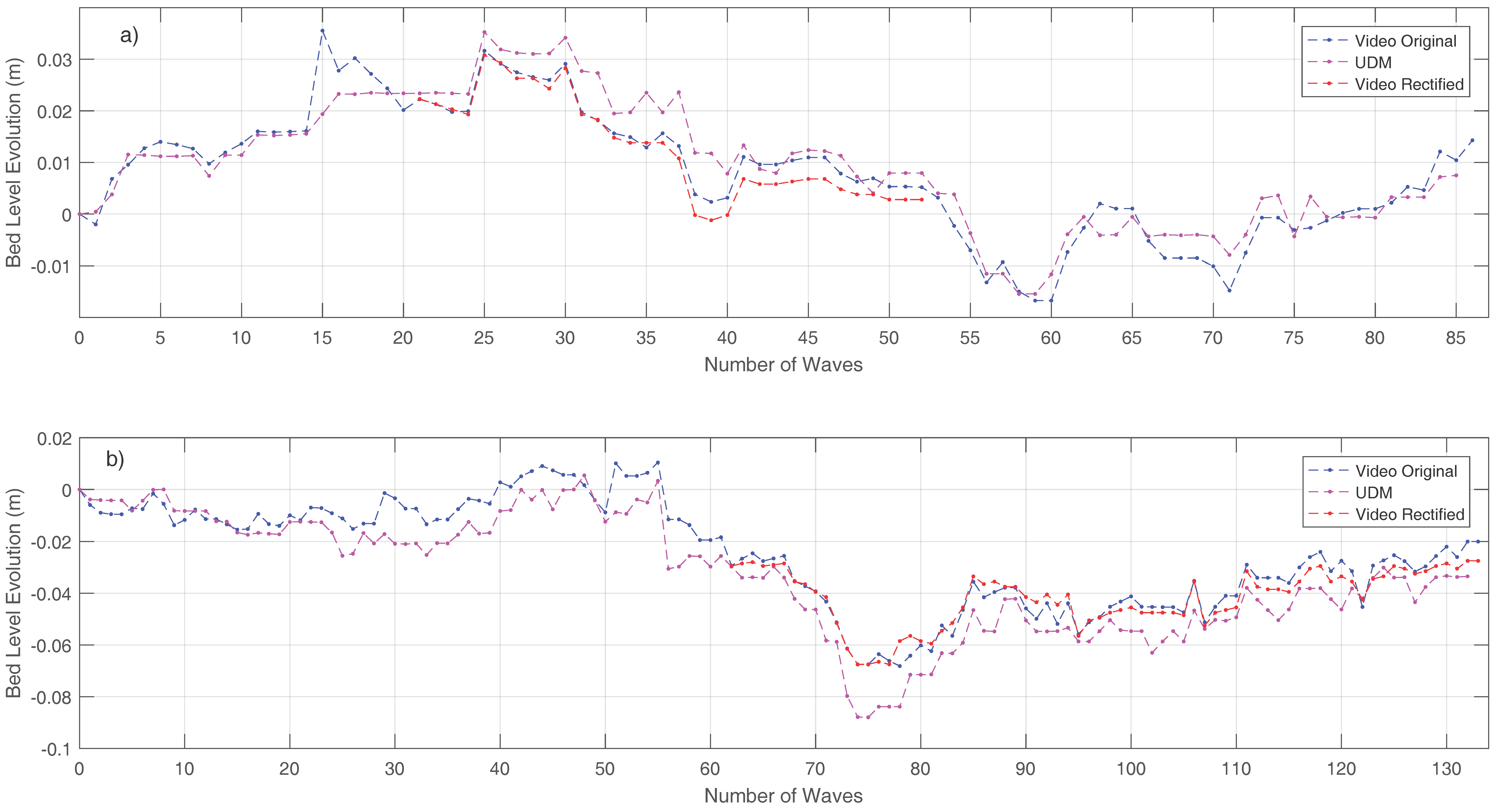
3.2. Comparison with Ultrasonic Distance Meters (UDM) for the Bed Level

Bed level extraction for UDM data is commonly accomplished by comparing the rate of change of bed elevation to some threshold (e.g., [15]). However, in this work, a variance threshold was used, similar to the processing used for the LiDAR data.
Figure 9a,c show 90 and 60 min synchronized time series of raw UDM (black dashed line) data along with extracted bed levels from the UDM (magenta solid line) and video (blue dashed line) data at the landward and seaward poles, respectively. The evolution of the bed level shows periods of erosion interrupted by periods of accretion. While a very good correlation between bed elevations measured by both instruments (cf. Table 2, R 2 = 0.89 0.93 ) and a low RMSE (0.0041–0.009 m) are obtained for the whole time series at both locations, the performance at the individual wave timescale shows more variability.
Histograms of wave-by-wave bed level changes Δ z are shown in Figure 10. It should be noted that the measurement resolution changes between poles according to Table 1, while it remains constant at 1 mm for the UDMs. At both locations, the histograms show a symmetrical distribution, with approximately equal numbers of erosion and accretion events. However, the video histogram is smoother than the UDM, which may be a result of the video accuracy and the sensitivity of the UDM sensor, as explained below.
The accumulated bed level evolution relative to the number of waves (swash events) is shown in Figure 11a for the landward pole over a 90 min window, where 86 waves were identified. The two sensors yield very similar trends with an overall consistency between erosion and accretion. However, individual events can vary significantly and show opposite behavior on occasion, consistent with the large Δ z values. Similar trends are found for the seaward position (Figure 11b, 132 waves in 60 min), and for longer time scales, from the group scale to hourly records encompassing the complete duration of the experimental dataset.

4. Discussion

The previous results show that bed and water levels obtained from the video technique and those from two conventional methods, show good agreement, especially in recovering trends at a range of time scales. This suggests that the simple and inexpensive setup described here is appropriate for obtaining swash data.
However, differences of up to the centimeter scale have been found for both bed and water surface levels. Differences were found to be greater at positions farther from the camera, probably due to a decreasing resolution. The problem is compounded for the Mataquito dataset, as LiDAR resolution also decreases with increasing distance between target and scanner [18].
In broad terms, the errors can be the result of several factors. For instance, problems arising from improper system set-up, or variations in the geometry of the system. For example, the comparison of bed levels show moderate agreement for both seaward and landward positions measured with LiDAR and video. LiDAR is known to be potentially affected by instabilities and vibrations of the supporting platform when measuring stationary targets, leading to errors of 2.5 mm [8] and standard deviations of up to 4.2 mm [18]. It is of note that RMSE errors fall within this order of magnitude.
The present method can be also affected by problems arising from installation. The method relies on the hypothesis that the poles belong to parallel imaginary planes; and that their short distance from the camera allows errors in collimation or lens distortion to be neglected. Finally, it is expected that the poles do not change their position relative to the camera.
To test these assumptions, checkerboards of known dimensions were placed atop the poles (landward and seaward poles, Figure 12a) during the Renãca experiments, and used as control points (Figure 12b). This enabled the errors in projecting a given pixel when the lens distortion is neglected to be assessed. A camera calibration routine to determine the intrinsic and extrinsic camera parameters was used, similar to the one proposed by Zhang [42] and implemented by Valentini et al. [43]. For the conditions and zoom setting used in Reñaca, this led to errors in placement that did not exceed one pixel. Therefore, for this particular case, the original assumption is valid, but other installations should consider estimating and accounting for these errors explicitly.
The checkerboard control points also enabled analysis of whether the vertical orientation of the pole was important. All image frames were subject to a projective 2D transformation that maps the images to the plane defined by the checkerboards. This rectification process ensures that the images comply with the orientation assumption (Figure 12c). Corrected time-space maps are then generated.
Bed levels were detected with the corrected time series and show a similar behavior than without rectifying (Figure 11a,b, red lines), with RMSE differences of 0.0015 m and 0.0028 m for the landward and seaward positions, respectively. Thus, the assumption that the the pole does not move enough to alter the mapping of a given pixel to the corresponding point in the pole is validated for this dataset. It should be noted that, whether rectification is performed or not, the method implicitly assumes that the pole does not shift location or orientation relative to the camera. In case of slight movements, correcting for it using the transformative projection can be performed on a frame-by-frame basis. This would require the top of the pole, or control points such as the checkerboard, to be tracked over time.
Slight pole rotations away from the vertical would not be expected to produce large discrepancies because the vertical change would be proportional to the ( 1 cos θ ) , where θ is the off-vertical rotation angle (e.g., [32]). To contextualize, a large 20 rotation will reduce the pixel resolution by 6%. While there are situations where the poles are displaced or rotated considerably from their original position, especially under energetic wave conditions, this could be reduced by proper burying. In Reñaca, a burying depth of 1 m produced good results. It is also noted that the camera orientation itself can drift. Therefore, it is also recommended that a solid and fixed camera clamping system (tripod) is used to ensure the stability of the camera during data collection.
The exact application of the algorithms used to detect the water and bed elevation can also cause some variability in the results. For example, while the water surface and bed level detection process becomes automatic once the values of the parameters α and β are determined, these values need to be estimated manually at each cross-shore location owing to their dependency on the presence of foam or sand over the time series. At seaward locations (e.g., Figure 2a), the presence of water accounts for a larger fraction of the pixel intensity along ξ = b o t t o m ¯ , increasing the mean and reducing the variance of optical intensity for I t h r B , when compared with landward locations (e.g., Figure 2c). Thus, seaward locations would require lower α values than landward locations. Here, a subset of the data (8 min) was used to manually estimate these values. This assumes that the sea state remains constant and thus swash frequency does not vary significantly over the course of the whole dataset. Within this subset, the number of bed level (dry) and water (wet) intervals are identified manually and numbered. The results are compared with those detected automatically using a range of α values. The final value of the parameter is taken as the α value which minimizes the error between manually and automatically detected results, and this is typically smaller than 5 percent, as seen in Figure 13. For the cases studied here, β = α 0.6 yields the best results for detecting the water surface. This is consistent with the expectation that the variance of the water level is larger due to the brighter colors of water, thereby requiring smaller thresholds.
One potential disadvantage of the video processing methodology is that the gradient of intensity between bed and pole comprises up to four pixels, therefore affecting the location of the maximum gradient. To analyze the sensitivity to this selection, the transition was modeled by fitting the time-averaged intensity to a sigmoidal function. The fitted expression is a logistic function
I ¯ ( ξ ) = I ¯ 1 + e ν ( ξ ξ ν ) ,
where I ¯ ( ξ ) is the time-averaged pixel intensity during an interval of bed level, I ¯ is the value of I ¯ ( ξ ) when ξ , ν is the decay constant and ξ ν is the coordinate defining the inflection and symmetry position of the function. We have carried out this analysis for the landward and seaward position of the Reñaca experiment due to greater availability of dry instants in between swash events.
For every bed level elevation found using the maximum gradient, a time series fitted with a logistic function is generated to compare ξ ν with the previous bed elevation. Figure 14a shows an example for the bed level detected using both approaches, and Figure 14b shows the fitted expression for one dry bed interval.
Figure 14c,d show bed level elevations obtained using the original video processing, using the logistic function (red lines) and also those derived from ultrasonic distance meters (magenta lines). Additionally, 95% confidence intervals of the logistic regression are shown in light blue, in order to account for the uncertainty in bed level detection.
At the landward position (Figure 14c), a maximum difference of two pixels, (∼3 mm) is found between the two optical methods. The seaward position (Figure 14d) shows larger differences on occasion, which is attributed to reduced contrast due to foggy conditions, but also to the decreased resolution due to the longer distance to the camera. These factors hampered the fitting of a logistic function due to noise in the time averaged pixel intensity. Despite this, most of the bed level elevations obtained by the original method and the logistic function differ less than four pixels (0.0076 m). Therefore, the overall accuracy of the data processing implemented here can be defined to four pixels (up to 1 cm for the present data set) when analyzing bed level.
Comparison of the water surfaces measured with video and LiDAR showed moderately good correlation, but differences are apparent locally. One possibility is that this is due to the use of the erosion–dilation filter. While the goal is to remove small scale features that might not be of hydrodynamic interest, detection without using the filter showed differences of up to 10 pixels, with the filter-less data yielding larger free surface elevations. Typical values were three pixels, and their overall occurrence was sporadic. The erosion filter is necessary to eliminate splashes, while removing dilation filter leads to larger disagreement between the video and the water surface observed in the time-space map (cf. Figure 5c), suggesting the use of the filter is appropriate.
More relevant appears to be the interference of the pole itself. Analysis of the full frame video shows that the pole affects the flow immediately local to it, producing a vertical flow structure around the pole’s shaft that yields overestimation of the water surface detected with video. These secondary flows are an additional rise in the water surface level due to conversion of kinetic to potential energy at the stagnation point on either side of the pole that are particularly evident during uprush. It is also noted that the uprush tends to be foamier and more easily distinguishable than backwash. This behavior is consistent with the tendency of video to overpredict the LiDAR time series. Owing to its physical origin, this effect cannot be reduced and it should be acknowledged when using the data.

5. Conclusions

This work assesses the performance of a video-based technique for monitoring bed and water surface levels of the swash zone at the scale of individual waves. The principle of the method is to monitor through video imaging, the elevation of the interfaces between water and sand against a known reference provided by several vertical poles buried in the sand. The method allows for different spatial configurations of the poles, provided each pole does not obstruct imaging of the others. Off-the-shelf video cameras can be used, mounted on tripods or other stable platforms, requiring minimal energy requirements and facilitating easy deployment. The main limitation of this system is the decreasing resolution as the reference is moved further away from the camera, which could reduce spatial coverage.
The results shown here indicate that ensuring a constant system geometry throughout data collection is beneficial. This can be achieved by proper burying of the poles, and by a stable camera support system. It is recommended that lens distortion effects are corrected for, and using checkerboards or other control points to track the camera and system geometry is suggested, although for short deployments where the poles remain stable this may not be required.
Regarding the expected accuracy of the method, measurements of water surface variations at the wave-by-wave scale proved to be accurate for the backwash phase (RMSE down to 0.028 m, R 2 up to 0.89), when compared against LiDAR data. However, larger discrepancies were found during the uprush phase (RMSE up to 0.062 m, R 2 down to 0.71), when the presence of the pole causes vertical flows generated upon the sudden arrival of the swash front.
Bed level evolution measurements compare well with conventional ultrasonic distance meters, reproducing erosion and deposition events at time scales ranging from wave groups to a longer (hourly) evolution. However, at the wave-by-wave scale, the method shows discrepancies principally attributed to a combination of the pixel resolution footprint and the identification of the bed level by image processing techniques, leading an estimated accuracy of O (1 cm).
As a result, when compared to other conventional techniques, the method offers comparable resolution capabilities. Owing to its simplicity of deployment, very low cost and reasonable accuracy, this technique can be adopted for swash data collection in the field.

Acknowledgments

Mataquito and Reñaca field experiments have been funded by the National Science and Technology of Chile, CONICYT by its acronym in spanish, through the FONDECYT project N1120878. Raimundo Ibaceta has been supported by the Centre National de la Recherche Scientifique, France (CNRS) through an internship grant, by CONICYT through the MSc. Scholarship CONICYT-PCHA/Magister Nacional/2015–22150007 and by DGIIP UTFSM. Rafael Almar was supported by French grant COASTVAR (ANR-14-ASTR-0019). The CONICYT/FONDAP/15110017 program, CONICYT/PIA/FB0821 and CONICYT/FONDECYT 1170415 are also acknowledged by Patricio A. Catalán. The authors would like to thank all the people involved in the field studies. Data and algorithms developed herein can be requested by contacting the authors.

Author Contributions

Raimundo Ibaceta deployed the ultrasonic distance meters and pole’s array at Reñaca with the assistance of Patricio Catalán, did the analysis related to data processing, comparison between instruments and wrote the article. Rafael Almar assisted during the LiDAR and pole’s deployment at Mataquito and contributed to the manuscript. Patricio A. Catalán contributed to the manuscript and assisted during both field experiments and during Raimundo’s analysis throughout his MSc. studies. Chris Blenkinsopp contributed to the manuscript and assisted the LiDAR deployment and provided its data. Luis P. Almeida contributed to the manuscript. Rodrigo Cienfuegos contributed to the manuscript and assisted during Mataquito field study.

Conflicts of Interest

The authors declare no conflict of interest. The founding sponsors had no role in the design of the study; in the collection, analyses, or interpretation of data; in the writing of the manuscript, and in the decision to publish the results.

References

  1. Elfrink, B.; Baldock, T. Hydrodynamics and sediment transport in the swash zone: A review and perspectives. Coast. Eng. 2002, 45, 149–167. [Google Scholar] [CrossRef]
  2. Masselink, G.; Puleo, J.A. Swash-zone morphodynamics. Cont. Shelf Res. 2006, 26, 661–680. [Google Scholar] [CrossRef]
  3. Brocchini, M.; Baldock, T.E. Recent advances in modeling swash zone dynamics: Influence of surf-swash interaction on nearshore hydrodynamics and morphodynamics. Rev. Geophys. 2008, 46. [Google Scholar] [CrossRef]
  4. Puleo, J.A.; Butt, T. The first international workshop on swash-zone processes. Cont. Shelf Res. 2006, 26, 556–560. [Google Scholar] [CrossRef]
  5. Hughes, M.G.; Masselink, G.; Brander, R.W. Flow velocity and sediment transport in the swash zone of a steep beach. Mar. Geol. 1997, 138, 91–103. [Google Scholar] [CrossRef]
  6. Blenkinsopp, C.; Turner, I.; Masselink, G.; Russell, P. Swash zone sediment fluxes: Field observations. Coast. Eng. 2011, 58, 28–44. [Google Scholar] [CrossRef]
  7. Puleo, J.; Lanckriet, T.; Blenkinsopp, C. Bed level fluctuations in the inner surf and swash zone of a dissipative beach. Mar. Geol. 2014, 349, 99–112. [Google Scholar] [CrossRef]
  8. Blenkinsopp, C.; Mole, M.; Turner, I.; Peirson, W. Measurements of the time-varying free-surface profile across the swash zone obtained using an industrial LIDAR. Coast. Eng. 2010, 57, 1059–1065. [Google Scholar] [CrossRef]
  9. Holman, R.; Guza, R. Measuring run-up on a natural beach. Coast. Eng. 1984, 8, 129–140. [Google Scholar] [CrossRef]
  10. Holland, K.T.; Raubenheimer, B.; Guza, R.T.; Holman, R.A. Runup kinematics on a natural beach. J. Geophys. Res. Oceans 1995, 100, 4985–4993. [Google Scholar] [CrossRef]
  11. Raubenheimer, B.; Guza, R.T.; Elgar, S.; Kobayashi, N. Swash on a gently sloping beach. J. Geophys. Res. Oceans 1995, 100, 8751–8760. [Google Scholar] [CrossRef]
  12. Masselink, G.; Russell, P. Flow velocities, sediment transport and morphological change in the swash zone of two contrasting beaches. Mar. Geol. 2006, 227, 227–240. [Google Scholar] [CrossRef]
  13. Cox, D.T.; Shin, S. Laboratory Measurements of Void Fraction and Turbulence in the Bore Region of Surf Zone Waves. J. Eng. Mech. 2003, 129, 1197–1205. [Google Scholar] [CrossRef]
  14. Lanckriet, T.; Puleo, J.A.; Masselink, G.; Turner, I.; Conley, D.; Blenkinsopp, C.; Russell, P. Comprehensive Field Study of Swash-Zone Processes. II: Sheet Flow Sediment Concentrations during Quasi-Steady Backwash. J. Waterway Port Coast. Ocean Eng. 2014, 140, 29–42. [Google Scholar] [CrossRef] [Green Version]
  15. Turner, I.L.; Russell, P.E.; Butt, T. Measurement of wave-by-wave bed-levels in the swash zone. Coast. Eng. 2008, 55, 1237–1242. [Google Scholar] [CrossRef]
  16. Masselink, G.; Russell, P.; Turner, I.; Blenkinsopp, C. Net sediment transport and morphological change in the swash zone of a high-energy sandy beach from swash event to tidal cycle time scales. Mar. Geol. 2009, 267, 18–35. [Google Scholar] [CrossRef]
  17. Baldock, T. Discussion of “Measurement of wave-by-wave bed-levels in the swash zone” by Ian L. Turner, Paul E. Russell, Tony Butt [Coastal Eng. 55 (2008) 1237–1242]. Coast. Eng. 2009, 56, 380–381. [Google Scholar] [CrossRef]
  18. Vousdoukas, M.; Kirupakaramoorthy, T.; Oumeraci, H.; de la Torre, M.; Wübbold, F.; Wagner, B.; Schimmels, S. The role of combined laser scanning and video techniques in monitoring wave-by-wave swash zone processes. Coast. Eng. 2014, 83, 150–165. [Google Scholar] [CrossRef]
  19. Almeida, L.; Masselink, G.; Russell, P.; Davidson, M. Observations of gravel beach dynamics during high energy wave conditions using a laser scanner. Geomorphology 2015, 228, 15–27. [Google Scholar] [CrossRef] [Green Version]
  20. Martins, K.; Blenkinsopp, C.E.; Zang, J. Monitoring Individual Wave Characteristics in the Inner Surf with a 2-Dimensional Laser Scanner (LiDAR). J. Sens. 2016, 83, 150–165. [Google Scholar] [CrossRef]
  21. Brodie, K.L.; Raubenheimer, B.; Elgar, S.; Slocum, R.K.; McNinch, J.E. Lidar and Pressure Measurements of Inner-Surfzone Waves and Setup. J. Atmos. Ocean. Technol. 2015, 32, 1945–1959. [Google Scholar] [CrossRef]
  22. Hofland, B.; Diamantidou, E.; van Steeg, P.; Meys, P. Wave runup and wave overtopping measurements using a laser scanner. Coast. Eng. 2015, 106, 20–29. [Google Scholar] [CrossRef]
  23. Aagaard, T.; Holm, J. Digitization of Wave Run-up Using Video Records. J. Coast. Res. 1989, 5, 547–551. [Google Scholar]
  24. Power, H.E.; Holman, R.A.; Baldock, T.E. Swash zone boundary conditions derived from optical remote sensing of swash zone flow patterns. J. Geophys. Res. Oceans 2011, 116. [Google Scholar] [CrossRef]
  25. Almar, R.; Blenkinsopp, C.; Almeida, L.P.; Cienfuegos, R.; Catalán, P.A. Wave runup video motion detection using the Radon Transform. Coast. Eng. 2017, 130, 46–51. [Google Scholar] [CrossRef]
  26. Holland, K.T.; Puleo, J.A. Variable swash motions associated with foreshore profile change. J. Geophys. Res. Oceans 2001, 106, 4613–4623. [Google Scholar] [CrossRef]
  27. Holland, K.T.; Holman, R.A. Video Estimation of Foreshore Topography Using Trinocular Stereo. J. Coast. Res. 1997, 13, 81–87. [Google Scholar]
  28. Astier, J.; Astruc, D.; Lacaze, L.; Eiff, O. Investigation of the Swash Zone Evolution At Wave Time Scale. Coast. Eng. Proc. 2012, 1, 48. [Google Scholar] [CrossRef]
  29. Astruc, D.; Cazin, S.; Cid, E.; Eiff, O.; Lacaze, L.; Robin, P.; Toublanc, F.; Cáceres, I. A stereoscopic method for rapid monitoring of the spatio-temporal evolution of the sand-bed elevation in the swash zone. Coast. Eng. 2012, 60, 11–20. [Google Scholar] [CrossRef]
  30. Chardón-Maldonado, P.; Pintado-Patino, J.C.; Puleo, J.A. Advances in swash-zone research: Small-scale hydrodynamic and sediment transport processes. Coast. Eng. 2016, 115, 8–25. [Google Scholar] [CrossRef]
  31. Mizuguchi, M. Swash on a Natural Beach. In Proceedings of the International Conference on Coastal Engineering, Houston, TX, USA, 3–7 September 1984; Volume 1. [Google Scholar]
  32. Ebersole, B.; Hughes, S. DUCK85 Photopole Experiment; Technical Report CERC-87-18; U.S. Army Waterways Experiment Station, Coastal Engineering Research Center: Vicksburg, MS, USA, 1987. [Google Scholar]
  33. Ebersole, B.; Hughes, S. SUPERDUCK Photopole Experiment; Draft Technical Report; U.S. Army Waterways Experiment Station, Coastal Engineering Research Center: Vicksburg, MS, USA, 1988. [Google Scholar]
  34. Weir, F.M.; Hughes, M.G.; Baldock, T.E. Beach face and berm morphodynamics fronting a coastal lagoon. Geomorphology 2006, 82, 331–346. [Google Scholar] [CrossRef]
  35. Larson, M.; Kubota, S.; Erikson, L. Swash-zone sediment transport and foreshore evolution: Field experiments and mathematical modeling. Mar. Geol. 2004, 212, 61–79. [Google Scholar] [CrossRef]
  36. Sallenger, A.H.; Richmond, B.M. High-frequency sediment-level oscillations in the swash zone. Mar. Geol. 1984, 60, 155–164. [Google Scholar] [CrossRef]
  37. Austin, M.J.; Masselink, G. Observations of morphological change and sediment transport on a steep gravel beach. Mar. Geol. 2006, 229, 59–77. [Google Scholar] [CrossRef]
  38. Austin, M.J.; Buscombe, D. Morphological change and sediment dynamics of the beach step on a macrotidal gravel beach. Mar. Geol. 2008, 249, 167–183. [Google Scholar] [CrossRef]
  39. Kulkarni, C.D.; Levoy, F.; Monfort, O.; Miles, J. Morphological variations of a mixed sediment beachface (Teignmouth, UK). Cont. Shelf Res. 2004, 24, 1203–1218. [Google Scholar] [CrossRef]
  40. Cienfuegos, R.; Villagran, M.; Aguilera, J.C.; Catalán, P.; Castelle, B.; Almar, R. Video monitoring and field measurements of a rapidly evolving coastal system: The river mouth and sand spit of the Mataquito River in Chile. J. Coast. Res. 2014, 26, 639–644. [Google Scholar] [CrossRef]
  41. Beyá, J.; Álvarez, M.; Gallardo, A.; Hidalgo, H.; Winckler, P. Generation and validation of the Chilean Wave Atlas database. Ocean Model. 2017, 116, 16–32. [Google Scholar] [CrossRef]
  42. Zhang, Z. A flexible new technique for camera calibration. IEEE Trans. Pattern Anal. Mach. Intell. 2000, 22, 1330–1334. [Google Scholar] [CrossRef]
  43. Valentini, N.; Saponieri, A.; Damiani, L. A new video monitoring system in support of Coastal Zone Management at Apulia Region, Italy. Ocean Coast. Manag. 2017, 142, 122–135. [Google Scholar] [CrossRef]
Figure 1. (a) LiDAR and a scaffold structure used for measurements at Mataquito; (b) pole array used in Mataquito field study; (c) instrument deployment at Reñaca Beach field study; (d) detail of a co-localized UDM used at Re ñaca; (e) cross-shore profile during the Mataquito field study; (f) cross-shore profile during the Reñaca field study. Black horizontal lines represent the maximum, mean and minimum water level during the experiment.
Remotesensing 10 00049 g001
Figure 2. Example of color (RGB) time-space images at three cross shore positions for the (a) lower swash (b) middle swash and (c) upper part of the beach. Each time series is 240 s in duration. Data are from Reñaca beach.
Remotesensing 10 00049 g002
Figure 3. (a) sample time-space image of approximately 240 s recorded at Reñaca. The colorbar corresponds to the grayscale pixel intensity, I ( ξ , t ) . Dashed lines represent the following ξ coordinates. Blue: pole top, green: o v e r b e d ¯ , magenta: b e d ¯ and cyan: b o t t o m ¯ ; (b) time-averaged gray scale intensity over the complete timestack.
Remotesensing 10 00049 g003
Figure 4. (a) sample time-space image in the lower swash zone at Renãca. Cyan dashed line denotes the pixel coordinate ξ = b o t t o m ¯ ; (b) pixel intensity time series at ξ = b o t t o m ¯ . The blue solid line indicates the threshold I t h r B = 164.4 (c) sample time-space image after application of I t h r B filter. Red dashed line is the bed level of the first dry interval between t = 0 and t = 19 s; (d) example of bed level detection for the first dry interval, showing the time-averaged pixel intensity over t = 0 and t = 19 s. The red dashed line represents the maximum gradient I ¯ ( ξ ) ξ ; (e) along-pole distribution of the gradient, I ¯ ( ξ ) ξ , estimated between t = 0 and t = 19 s. Red square denotes the maximum value.
Remotesensing 10 00049 g004
Figure 5. (a) sample time-space map upon application of I t h r W ; (b) noise and splashes are reduced after the application of an erosion–dilation filter; (c) final detection of the bed level (red dashed line) and water surface (magenta dashed line). In addition, water surface detected using only an erosion filter is shown in yellow solid line. (see Discussion below).
Remotesensing 10 00049 g005
Figure 6. Thirty-minute time series of LiDAR (red dashed line) and video (black solid line) measured in Mataquito Beach at the (a) landward position and (b) seaward position. Five-minute subsets of the data are also shown at the (c) landward position and (d) seaward position.
Remotesensing 10 00049 g006
Figure 7. Scatter plots of the water surface elevation obtained with LiDAR and the pole method at Mataquito, with the uprush and backwashes phases separated. Blue solid lines are the fitted regression lines, cyan lines are the regression lines with 95% confidence interval; and black dashed line denotes perfect fit (1:1). (a) uprush landward pole R 2 = 0.71 ; (b) backwash landward pole R 2 = 0.85 ; (c) uprush seaward pole R 2 = 0.81 ; (d) backwash seaward pole R 2 = 0.89 . See Table 2 for a summary of error statistics.
Remotesensing 10 00049 g007
Figure 8. Cumulative bed level change as a function of the number of waves (swash events) measured at both cross-shore positions (a) landward and (c) shoreward. Red and black solid lines are bed level evolution derived from LiDAR and video, respectively. Bed level evolution starts from the 0 m elevation for the first wave. Scatter plots of the bed level elevation in between swash events are shown for the (b) landward and (d) seaward positions. Blue solid lines are the fitted regression lines, cyan lines are the regression lines with 95% confidence interval; and black dashed line denotes perfect fit (1:1).
Remotesensing 10 00049 g008
Figure 9. Comparison between UDM and video records. Black solid lines are the raw UDM measurements. Bed levels for the video method (blue dashed line) and UDM (magenta solid line) are also shown for the (a) landward (90 min) and (c) seaward (60 min) poles. Only 60 min of synchronized measurements are shown for the seaward position, but 90 min are present for the UDM measurements to match with the duration of the landward position. Scatter plots of the bed level elevation in between swash events are shown for the (b) landward and (d) seaward positions. Blue solid lines are the fitted regression lines, cyan lines are the regression lines with 95% confidence interval; and the black dashed line denotes the perfect fit (1:1).
Remotesensing 10 00049 g009
Figure 10. Histograms of bed elevation changes at the wave-by-wave timescale Δ z for the (a) landward and (b) shoreward pole position.
Remotesensing 10 00049 g010
Figure 11. Cumulative bed level evolution as a function of the number of waves (swash events) recorded at both cross-shore positions (a) landward and (b) shoreward. Magenta lines represent the UDM data, blue lines show the video method as proposed in this work and the red line presents the results for the rectified video method outlined in the discussion.
Remotesensing 10 00049 g011
Figure 12. 2D projective transformation; (a) original frame; (b) control points (red circles) used in the landward pole for the rectification; (c) rectified frame. Stacking over each pole and bed level detection is done after this stage for comparison between the original and rectified video records as shown in the red lines of Figure 11a,b.
Remotesensing 10 00049 g012
Figure 13. Selection of α value (solid red circle) that minimizes the relative error between the number of automatically detected and manually selected bed intervals at the cross-shore positions (a) low swash zone (Figure 2a), α = 1.6 ; (b) middle swash (Figure 2b) α = 2 ; and (c) upper part of the beach (Figure 2c) α = 2.4 .
Remotesensing 10 00049 g013
Figure 14. Bed level detection using two approaches. (a) timestacks and bed level detected by means of the maximum I ¯ ( ξ ) ξ (red dashed line) and by fitting a sigmoidal function of the averaged pixel intensity I ¯ ( ξ ) for each dry interval (green dashed line). (b) sample detection for a bed level interval in between swash events. Black solid line is the pixel intensity I ¯ ( ξ ) and the magenta dashed line is the corresponding sigmoidal fit. The red circle is the position of maximum gradient, while the green circle is the inflexion point of the fitted function. For this example, both methods yield the same results. Light blue solid plot is the logistic regression fit with 95% confidence interval. The bed level elevation derived from the original video method (bed lines), logistic function (red line) and UDM (magenta lines) are shown for the (c) landward and (d) seaward position. Light blue solid envelopes are the 95% confidence interval of the bed level derived from the logistic function.
Remotesensing 10 00049 g014
Table 1. Vertical pixel resolutions for both experiments.
Pole LocationResolutionPole LocationResolution (m/pixel)
(Mataquito)(m/pixel)(Reñaca)(Reñaca)
Landward0.0026Landward0.0015
Seaward0.0032Seaward0.0019
Table 2. Summary of statistical analysis for both experiments. a and b are the slope and intercept of the fitted regression η Video = a η LiDAR + b .
MataquitoReñaca
Pole-DataRMSE (m) R 2 abRMSE (m) R 2 ab
Landward Overall0.023-------
Landward Uprush0.0500.71−0.2371.414----
Landward Backwash0.0280.850.0280.994----
Landward Bed level0.0040.820.3180.8160.0040.890.1270.940
Seaward Overall0.044-------
Seaward Uprush0.0620.810.0370.986----
Seaward Backwash0.0370.890.2120.863----
Seaward Bed level0.0050.690.0910.9330.0090.930.2430.87

