Improving Selection of Spectral Variables for Vegetation Classification of East Dongting Lake, China, Using a Gaofen-1 Image


1
Research Center of Forest Remote Sensing & Information Engineering, Central South University of Forestry & Technology, Changsha 410004, China
2
Key Laboratory of Forestry Remote Sensing Based Big Data & Ecological Security for Hunan Province, Changsha 410004, China
3
Department of Geography and Environmental Resources, Southern Illinois University, Carbondale, IL 62901, USA
*
Authors to whom correspondence should be addressed.
Remote Sens. 2018, 10(1), 50; https://doi.org/10.3390/rs10010050
Submission received: 8 November 2017
/
Revised: 24 December 2017
/
Accepted: 28 December 2017
/
Published: 29 December 2017
Abstract
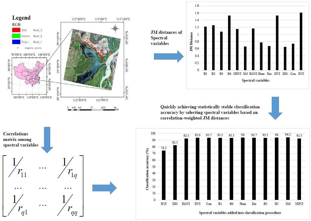
:There is a large amount of remote sensing data available for land use and land cover (LULC) classification and thus optimizing selection of remote sensing variables is a great challenge. Although many methods such as Jeffreys–Matusita (JM) distance and random forests (RF) have been developed for this purpose, the existing methods ignore correlation and information duplication among remote sensing variables. In this study, a novel approach was proposed to improve the measures of potential class separability for the selection of remote sensing variables by taking into account correlations among the variables. The proposed method was examined with a total of thirteen spectral variables from a Gaofen-1 image, three class separability measures including JM distance, transformed divergence and B-distance and three classifiers including Bayesian discriminant (BD), Mahalanobis distance (MD) and RF for classification of six LULC types at the East Dongting Lake of Hunan, China. The results showed that (1) The proposed approach selected the first three spectral variables and resulted in statistically stable classification accuracies for three improved class separability measures. That is, the classification accuracies using three or more spectral variables statistically did not significantly differ from each other at a significant level of 0.05; (2) The statistically stable classification accuracies obtained by integrating MD and BD classifiers with the improved class separability measures were also statistically not significantly different from those by RF; (3) The numbers of the selected spectral variables using the improved class separability measures to create the statistically stable classification accuracies by MD and BD classifiers were much smaller than those from the original class separability measures and RF; and (4) Three original class separability measures and RF led to similar ranks of importance of the spectral variables, while the ranks achieved by the improved class separability measures were different due to the consideration of correlations among the variables. This indicated that the proposed method more effectively and quickly selected the spectral variables to produce the statistically stable classification accuracies compared with the original class separability measures and RF and thus improved the selection of the spectral variables for the classification.

1. Introduction
Classification of land use and land cover (LULC) types using images is a basic and important application of remote sensing technologies and substantial research has been conducted. However, classification accuracy greatly varies depending on many factors. The factors include spectral signature of targets, background land covers, image selection, determination of spatial resolution, image preprocessing and enhancement, extraction of remote sensing variables, correlation and information duplication among remote sensing variables, selection of classifiers such as parametric and non-parametric methods, landscape complexity, etc. Thus, accurately classifying remotely sensed images into LULC maps is still challenging [1,2,3,4,5]. This study focused on exploring the development of a novel method that can be used to improve the selection of remote sensing variables for image classification of LULC types given other factors such as a study area, a data set, a classifier, etc., are held constant.
Selecting and combining remote sensing variables is critical for implementing an accurate classification [3]. Selection of remote sensing variables greatly varies depending on available bands or channels from airborne and space borne sensors. In addition to the bands from sensors, a large number of remote sensing variables can be derived by conducting various image enhancements and transformations, including image ratios, vegetation indices, image transformations, textural or contextual features and data fusion [1,2,6]. Moreover, principal component analysis, minimum noise fraction transform, decision boundary feature extraction, wavelet transform, Fourier analysis or transform and spectral mixture analysis can also be used to create remote sensing variables and to reduce data redundancy [7,8,9,10].
The availability of a large number of remote sensing variables have caused the difficulty to select useful variables. Thus, how to select the remote sensing variables that significantly contribute to increasing accuracy of distinguishing LULC types becomes very important. When the number of remote sensing variables is relatively small, simple and traditional methods such as bar graph spectral plots and feature space plots are usually utilized. In the case of a large number of remote sensing variables, statistical methods such as optimal index factor (OIF) and average divergence are employed to identify an optimal subset of remote sensing variables [1]. Complicated methods include fuzzy-logic expert system, exhaustive search by recursion, isolated independent search and sequential dependent search for optimizing the selection of remote sensing variables [11,12]. In addition, Bhattacharyya distance and Jeffreys–Matusita (JM) distance have been widely used to measure the ability of remote sensing variables for separating LULC types and selecting significant remote sensing variables [1,13,14,15,16,17,18,19,20].
Remote sensing variables have their characteristics and capacities of class separability. Different combinations may lead to great differences of classification accuracy due to interactions and correlations among remote sensing variables. Given other factors such as a data set and classifier that affect classification accuracy are held constant, finding a combination of remote sensing variables that can lead to highest classification accuracy will be very critical. For example, given a requirement of classification accuracy, how many remote sensing variables are enough? Whether or not using too many remote sensing variables will result in decrease of classification accuracy due to uncertainty of input variables? How do remote sensing variables interact with each other? How do correlations among remote sensing variables affect classification accuracy? On the other hand, the ratio of the number of input variables to the number of training samples is also critical for parametric classification methods. Currently, there have been no general standards or rules used to search for an optimal solution. There have also been no effective methods that can be utilized to optimize the selection of remote sensing variables in the case of multi-collinearity.
Principal component analysis (PCA) is a most widely used method to reduce the information redundancy of remote sensing variables by linearly combining original variables and transforming them into a set of new un-correlated variables. This means that PCA does not directly rank and select remote sensing variables. The new variables derived by PCA are not bio-physically meaningful. As the number of remote sensing variables and their spatial resolutions increase, PCA will also become very intensive for computation. Moreover, a machine learning algorithm–random forests (RF) has been widely used for classification of LULC types [21,22,23,24,25,26,27]. This method has the ability of optimizing both classification results and selection of remote sensing variables. For example, Hao et al. [24] used the score values of variable importance from RF to conduct feature selection of time series MODIS data and early crop classification. However, RF is a very complicated algorithm and its classification accuracy varies depending very much on the use of a large amount of training data. RF also lacks the ability of effectively taking into account correlations among remote sensing variables for quantifying the importance of variables.
The objective of this study was to develop an improved class separability-based method to select remote sensing variables derived from images for classification of LULC types. The improved method takes into account correlations among remote sensing variables, weights class separability measures with the inverse values of correlation coefficients, thus reduces the effects of correlations on classification accuracy and improves the selection of remote sensing variables. This method was validated in the East Dongting Lake of Hunan, China, to implement wetland classification using three widely used class separability measures including JM distance, transformed divergence and B-distance and three classifiers including two traditional parametric methods: Bayesian discriminant (BD) and Mahalanobis distance (MD) and a nonparametric machine learning algorithm: RF.
2. Materials and Methods
2.1. Study Area
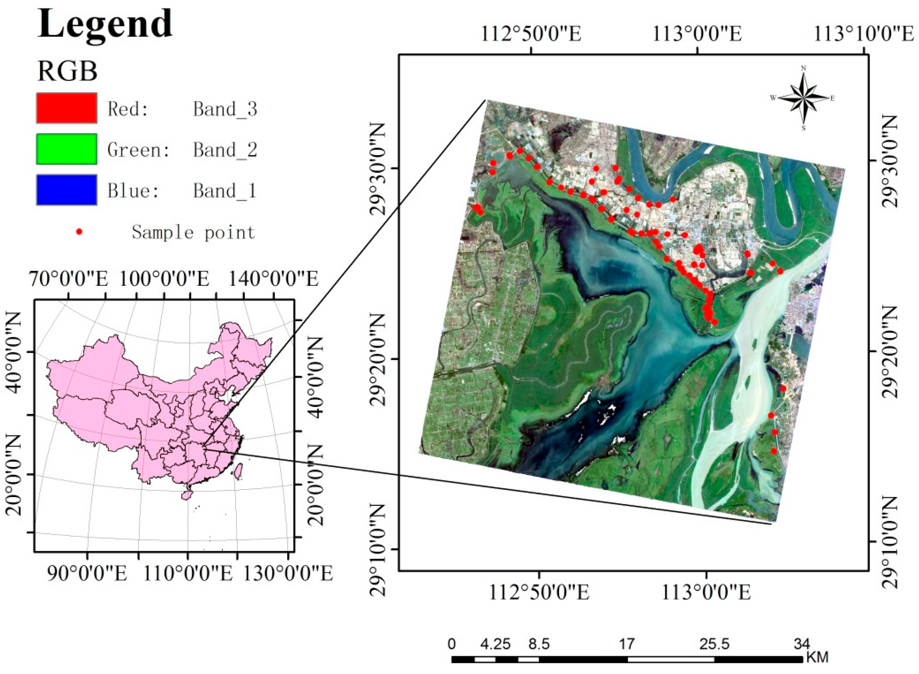
Dongting Lake located in Northeastern Hunan is the second largest freshwater lake in China. It consists of the East Dongting Lake, the West Dongting Lake and the South Dongting Lake. This study was conducted in the East Dongting Lake–the biggest sub-system of the Dongting Lake (Figure 1). The East Dongting Lake connects the Yangtze River and functions as a flood basin. The size of the East Dongting Lake thus varies seasonally.
The East Dongting Lake with a total area of about 190,000 hectares has the latitude and longitude ranges of 28°59′N to 29°38′N and 112°43′E to 113°15′E, respectively (Figure 1). This area is within a typical subtropical climate region with an average annual temperature of 17 °C and an annual precipitation of 1250 mm. Its elevation varies from 10 m to 80 m above sea level. The study area is dominated by water bodies, vegetated wetlands and bare lands. Major plant species include carex, phragmites or reed, poplar and willow. The East Dongting Lake as a National Nature Reserve is diverse in species of plants, birds and fish.
During the past fifty years the wetlands of the East Dongting Lake have experienced dramatically changes [28]. In 1970s and 1980s, the lake greatly shrank due to the expansion of agricultural land. After a great flood taking place in 1998, Hunan government shifted the emphasis of agricultural land use to protection of wetlands in the Dongting Lake basin, which led to an increase of the East Dongting Lake area. In 1990s and 2000s, however, the construction of the Three Gorges Dam reduced the area of the East Dongting Lake again because the Dam stores water during the rain seasons. Several authors have studied the classification of the Dongting Lake (including the East Dongting Lake) wetlands and their dynamics using optical remote sensing data and traditional classification methods such as supervised classification and object-oriented classification [29,30,31,32]. However, there is a lack of methods used to improve the selection of remote sensing variables and classification accuracy of the wetlands.
2.2. Sample Plot Data
With the help of an old LULC map [31,32], a Gaofen-1 (GF-1) image and a field survey, this study area was divided into six land cover types including water bodies, bare lands and four vegetation types (carex, phragmites or reed, poplar and willow). The old LULC map was consistent with the image and field survey in time of year and season. A total of 1200 sample plots with a size of 5 m × 5 m were selected from six land cover types each with 200 sample plots. Due to the existence of water bodies, some of the study area had no access by wheel vehicles. In order to save time and make sure of statistical reliability, we first searched for an area with access available–a belt from the northwest to the east part of the study area in which all the land cover types were found. The sample plots were then randomly allocated within each of six land cover types along the belt. All the sample plots were investigated in August of 2014 and their land cover types were determined. The sample plots were shown in the GF-1 image (Figure 1). For each land cover type, 100 sample plots were used as training data and the rest 100 sample plots as validation data. The spectral values of the sample plots at which the observations of six land cover types were collected were extracted using the average values of the pixels in the windows similar to the plots in size from sharpened GF-1 image bands and their enhanced spectral images mentioned below. We used the plot size of 5 m × 5 m mainly because this was the dominant size of the land cover types scattered in the water bodies of this area and would help to accurately extract the characteristics of the land cover types.
2.3. Gaofen-1 Image and Transformations
In this study, an image dated on 1 May 2014 was acquired from GF-1 satellite. Because of lack of cloud-free images, this image was three months older than the field data collected in August. However, in Hunan of China, vegetation starts growing at the beginning of April and both the image and field data were collected in the same rain season. Thus, it was expected that the difference of three months could not lead to a large uncertainty of the land cover classification.
GF-1 was launched on 26 April 2013 and is the first one of the high-resolution Chinese Earth Observation Satellite series to provide near-real-time observations for disaster prevention and relief, climate change monitoring, geographical mapping, environmental and resource surveying, as well as precision agriculture. GF-1 is equipped with two 2 m Pan/8 m multi-spectral cameras and a four 16 m multi-spectral medium-resolution and wide-field camera set. These two kinds of cameras provide images with the nadir swath widths of 69 km and 830 km, respectively. GF-1 was designed for a life of 5 years with an imaging capacity at both medium and high spatial resolution and a temporal resolution of 4 days or less. The images have a radiometric resolution of 10 bits.
The image acquired in this study covered the whole study area of 35 km × 35 km. The image consisted of four multi-spectral bands at an 8 m spatial resolution, including band 1-Blue: 0.45–0.52 µm, band 2-Green: 0.52–0.59 µm, band 3-Red: 0.63–0.69 µm and band 4–Near Infrared (NIR): 0.77–0.89 µm and one panchromatic band at a 2 m spatial resolution: 0.45–0.90 µm. The radiometric and atmospheric corrections of the images were carried out using ENVI radiometric calibration and FLAASH atmospheric correction tool. The digital numbers of the pixels were first converted to the values of spectral radiance at the sensor’s aperture and at-satellite reflectance using the satellite parameters and solar zenith angles and then converting the satellite reflectance values to the reflectance values at ground surface. Because the study area was flat, reducing the effects of slope, aspect and shade on the image was not made. The image was finally geo-referenced to the Universal Transverse Mercator (UTM) projection and coordinate system with an allowed root mean square error less than one pixel. In addition, the multi-spectral bands were sharpened with the panchromatic band using the Brovey transformation, leading to four 2 m spatial resolution bands: band 1-B1, band 2-B2, band 3-B3 and band 4-B4. The sharpened bands were then scaled up to a 4 m spatial resolution using a window average method and used for classifying the land cover types. The up-scaled bands had the size of pixels that was close to the size of the sample plots. Moreover, after the pan-sharpening, the information of the multi-spectral bands was enhanced because the panchromatic band had a 2 m spatial resolution and more details of ground objects. The pan-sharpened multi-spectral bands could help identify the land cover types for the field work.
In addition to the sharpened GF-1 image bands used, following B4 relevant vegetation indices, including normalized difference vegetation index (NDVI): (B4 − B3)/(B4 + B3), red green vegetation index (RGVI): (B3 − B2)/(B3 + B2), difference vegetation index (DVI): B4 − B3 and ratio vegetation index (RVI) (B4/B3) [1,2,3] were calculated to capture vegetation canopy features and structures. The reason for using the B4 relevant vegetation indices was mainly because B4 is a near infrared band and can characterize not only the canopy features and structures of different plant species in the wetland environment but also the borders of the water bodies from the lands. In order to quantify the image textures, texture measures of the B4 relevant spatial-dependency gray level co-occurrence matrices (GLCM) [6], including second moment (SM), homogeneity (Hom), entropy (Ent), dissimilarity (Dis) and contrast (Con), were also derived. Thus, a total of thirteen remote sensing variables were used and called spectral variables next because they were obtained from the GF-1 optical image.
2.4. Improving Selection of Spectral Variables
The importance of a spectral variable in classification of LULC types can be measured based on its ability of distinguishing the types. In this study, the ability of each spectral variable to distinguish six land cover types, including water bodies, bare lands, carex, phragmites or reed, poplar and willow, was quantified using three widely used measures of class separability, including JM distance [13,14,16,17,18,19,20], transformed divergence [1,17,33,34] and B-distance [35]. The class separability measures were used to rank the spectral variables that were input one by one into the set of the spectral variables used for classifying the six land cover types. JM distance between two land cover types c and d was defined as follows:
where is Bhattacharyya distance between land cover types c and d; and are the mean vectors of the types c and d, respectively; and and are the covariance matrices for the two types c and d, respectively; is the transpose of the difference vector; is the inverse of the covariance matrix; is the determination of the covariance matrix. In the case of more than two categories, JM distance is used as an average distance calculated based on mean vectors and covariance matrices of spectral variables to quantify the potential class separability of LULC types. JM distance has a range of 0 to 2, implying the potential accuracy of classification. The JM distance values smaller than 1.8 usually indicate low separability. The greater the JM distance, the higher the potential class separability [15].
Transformed Divergence (simply called divergence next) is defined as and similar to JM distance with a range of 0 to 2, in which D is calculated as a divergence based on mean vectors and covariance matrices of spectral variables [1,17,33,34,35,36]:
where tr[] is the trace of a matrix (i.e., the sum of the diagonal elements).
For one spectral variable i, B-distance for any two land cover classes, , can be first calculated using an absolute value of summation of spectral mean values divided by the sum of their variances [35]. An average value of all the distances for the spectral variables and all possible class-pairs is then derived and used.
Spectral variables are often correlated with each other, which leads to information duplication and impedes the increase of classification accuracy of LULC types. The above class separability measures quantify the ability of spectral variables to distinguish LULC types without consideration of correlations among spectral variables. In this study, a novel method to improve the selection of spectral variables for classification of the six land cover types was proposed. This method weighted the distances calculated above with the absolute inverse values of Pearson product moment correlation coefficients among spectral variables to quantify their contributions to improving classification accuracy when the spectral variables were selected for classification. It was in detail described next using JM distance as an example. Suppose the number of the spectral variables is q, and their average JM distances are .
- (1)
- The mean values of JM distances were utilized to rank the spectral variables for their abilities of distinguishing the land cover types. The most important spectral variable with the largest mean JM distance value was first selected to conduct the classification of the land cover types. This spectral variable was denoted with .
- (2)
- To select the second important spectral variable to be added for the classification, the correlation coefficient between each of the left q−1 spectral variables with the involved spectral variable was calculated:
The higher the correlation, the more the information duplicated. The absolute values of the correlation coefficients were inversed and then timed with their mean values of JM distances, . The resulting value was called correlation-weighted JM distance. The greater the value, the less the duplicated information and thus the greater the class separability ability. The spectral variable that had the largest correlation-weighted JM distance, denoted with , was selected and added for classifying the land cover types.
- (3)
- To select the third important spectral variable to be added for the classification, the correlation coefficients of the left q − 2 spectral variables with the involved spectral variables and , were respectively calculated and their absolute inverse values of the correlation coefficients were then derived and timed with their mean JM distances. The spectral variable with the largest correlation-weighted JM distance, denoted with , was selected and added for the classification.
- (4)
- The above step 3 was repeated and , , …, were ranked and sequentially added for the classification.
The aforementioned method led to correlation-weighted JM distances and improved JM distance based class separability measure. Similar to the modification of JM distance, the improved divergence and B-distance based class separability measures were developed. The improved class separability measures were compared with the original ones for selecting the spectral variables and conducting the classification. Two traditional parametric classifiers BD and MD and a non-parametric method RF, were used and compared to classify the East Dongting Lake into six land cover types: willow forests, poplar forests, reed areas, carex areas, water areas and built-up and exposed areas.
The three classifiers have been widely used for classification of LULC types and the details of the methods were omitted in this study. Here, we just simply described the machine learning algorithm RF. RF [21,22,23,24,25,26,27] constructs many classification trees by randomly sampling training data with replacement. For each of the trees, about two-third sample data are selected as training data and the left one-third sample data are used as validation data. At the same time, a subset of spectral variables can be randomly selected. Each tree outputs a classification result and the majority of class estimates from all the classification trees is then used as the prediction of classification. RF has the ability of optimizing selection of spectral variables by calculating the mean decrease in accuracy before and after a spectral variable is permuted. Thus, RF can optimize both selection of spectral variables and the estimates of classification. In this study, we first tested the sensitivity of the number of the used classification trees (ntree) and the number of the selected spectral variables based on the change of out-of-bag (OOB) error and classification accuracy. We then used RF to complete following calculations: (1) all classifications of six land cover types for the study area using the sets of the spectral variables selected based on the values of the improved JM distance, divergence and B-distance; (2) the importance scores of all the spectral variables; (3) the classification of six land cover types using the important spectral variables derived by RF but significant correlations among the variables may exist; and (4) the classification of six land cover types using the spectral variables that were important but not significantly correlated with each other. We then compared the proposed method with RF for both selections of spectral variables and the results of classification.
A total of 600 sample plots were used as training samples and other 600 sample plots as validation samples. A simple percentage of correctly classified sample plots was utilized for assessing the accuracy of classification. The statistically significant differences of classification accuracies obtained from any two methods were examined using the frequency based significant difference test at the significant level of 0.05 and with the sample size of 600 validation plots.
3. Results
3.1. Correlations among Spectral Variables
The absolute values of Pearson product moment correlation coefficients among 13 spectral variables were listed in Table 1. The spectral variables were highly correlated with each other within each of the groups: the original bands B1, B2 and B3; the B4 relevant vegetation indices NDVI, DVI, RVI and B4; and the texture measures from B4: SM, Hom, Ent, Dis and Con. The texture measures had low correlations with the original bands and their vegetation indices except having a moderate correlation with NDVI. The original bands: B1, B2 and B3, were moderately correlated with the vegetation indices. Overall, based on the critical value of 0.086 at the significant level of 0.05 and with the sample size of 600, most of the correlations were statistically significantly different from zero and thus should be considered when the spectral variables were selected for the classification of six land cover types in this study.
3.2. Improving Selection of Spectral Variables for Classification
3.2.1. JM Distance and Correlation-Weighted JM Distance
In Figure 2a, the average JM distances for distinguishing six land cover types showed that among the 13 spectral variables, RVI had the largest potential class separability ability, then B4, DVI, B2, B1, RGVI, NDVI, B3, Hom, Con, Ent, SM and Dis. This rank implied that both the original bands and vegetation indices had larger values of JM distances, indicating greater potential class separability, than the texture measures mainly because the formers captured the features and structures of spectral reflectance from the vegetation canopy, bare soils and water bodies. On the other hand, the texture measures did not well characterize the image textures probably because the canopy structures of the wetland plants were relatively simple and looked smoothing in the GF-1 image because the spatial resolution of the original multi-spectral bands was relatively coarse although the multi-spectral B4 used to calculate the texture measures was pan-sharpened.
The classification of six land cover types was first conducted using BD classifier by adding the spectral variables orderly based on their average JM distances. When RVI alone was used for classifying the six land cover types, an overall accuracy of 74.3% was obtained (Figure 2b). When B4 was added, the overall accuracy increased to 85.3%. However, adding DVI resulted in a slight decrease of the accuracy to 83.2% because of the high correlation between DVI and RVI. Similarly, introducing B2 led to the increase of the accuracy to 88.8% but the overall accuracy dropped down to 88.2% after adding B1 because of the high correlation between B1 and B2. The addition of RGVI resulted in an overall accuracy of 92.7%, a great increase of classification accuracy, because RGVI was weakly correlated with all the selected spectral variables. Further introducing NDVI and B3 decreased the overall accuracy to 91.0% because of information duplication caused by the high correlations of NDVI with RGVI, DI and RVI and of B3 with bands 1 and 2. After that, as the texture measures Hom, Con, Ent, SM and Dis were introduced into the classification procedure, the classification accuracy only slightly fluctuated with a range of 92.0% to 92.8% (Figure 2b). The greatest accuracy of 92.8% was obtained by using a total of 11 spectral variables. Overall, based on the statistical test of significant difference of the classification accuracies as frequencies, when the number of the selected spectral variables was equal to or larger than 6, the obtained accuracies did not significantly differ from each other at the significant level of 0.05 and could be called as statistically stable classification accuracies.
Figure 3a showed the importance rank of the left 12 spectral variables after the first spectral variable RVI and their correlation-weighted JM distances. When the first spectral variable RVI was added, no correlation needed to be considered and its selection was determined based on the original JM distance above. Starting from the second spectral variable added, the correlation-weighted JM distances of all the left spectral variables related to the first added spectral variable were calculated and the spectral variable that had the greatest distance was chosen. After the second spectral variable was added, the correlation-weighted JM distances of all the left spectral variables related to the first and second added spectral variables were calculated and the third spectral variable was identified and added based on the largest correlation-weighted JM distance. This process continued until all the spectral variables were ranked. The obtained importance rank of the spectral variables shown along the x-axis of Figure 3a differed from that based on the original JM distances. After RVI was added, among the left 12 spectral variables, texture measure Dis had the greatest correlation-weighted JM distance and was chosen as the second spectral variable added into the classification procedure. After that, the rank of the selected spectral variables was RGVI, DVI, Con, B1, B4, Hom, Ent, B3, B2, SM and NDVI, which were orderly added (Figure 3a).
In Figure 3b, the classification results of six land cover types were produced by selecting the spectral variables into the classification procedure based on the improved class separability values: correlation-weighted JM distances. When the first variable RVI was used for the classification, an overall accuracy of 74.3% was obtained and the same as that with the original JM distance. The addition of Dis and RGVI increased the overall accuracy of classification to 82.5% and 92.5%, respectively and further introducing DVI led to the accuracy increased to 93.0%. This implied that when the correlation-weighted JM distances were utilized, the overall accuracy from the first 4 spectral variables was greater than the largest accuracy obtained using 11 spectral variables when the original JM distances without the correlation-weighting were utilized. As more spectral variables were added, the classification accuracy slightly fluctuated with the maximum value of 94.2% created using a total of 12 spectral variables. However, the statistically stable classification accuracies started to be obtained after the first three spectral variables.
3.2.2. Divergence and Correlation-Weighted Divergence
In Figure 4a, the important rank of 13 spectral variables obtained using the original divergences was similar to that using the original JM distances above. The greatest class separability was obtained by RVI, then DVI, B1, B2, B4, NDVI, B3, RGVI, Con, Hom, SM, Ent and Dis. The only differences were the orders of B1, B2, B3 and B4. Figure 4b showed that as the number of the spectral variables introduced into classification procedure increased, the overall classification accuracy obtained using BD classifier continuously increased up to the largest accuracy of 92.8% created when the 11th spectral variable SM was added. However, it was found that overall, the statistically stable classification accuracies started to be created after the first eight spectral variables.
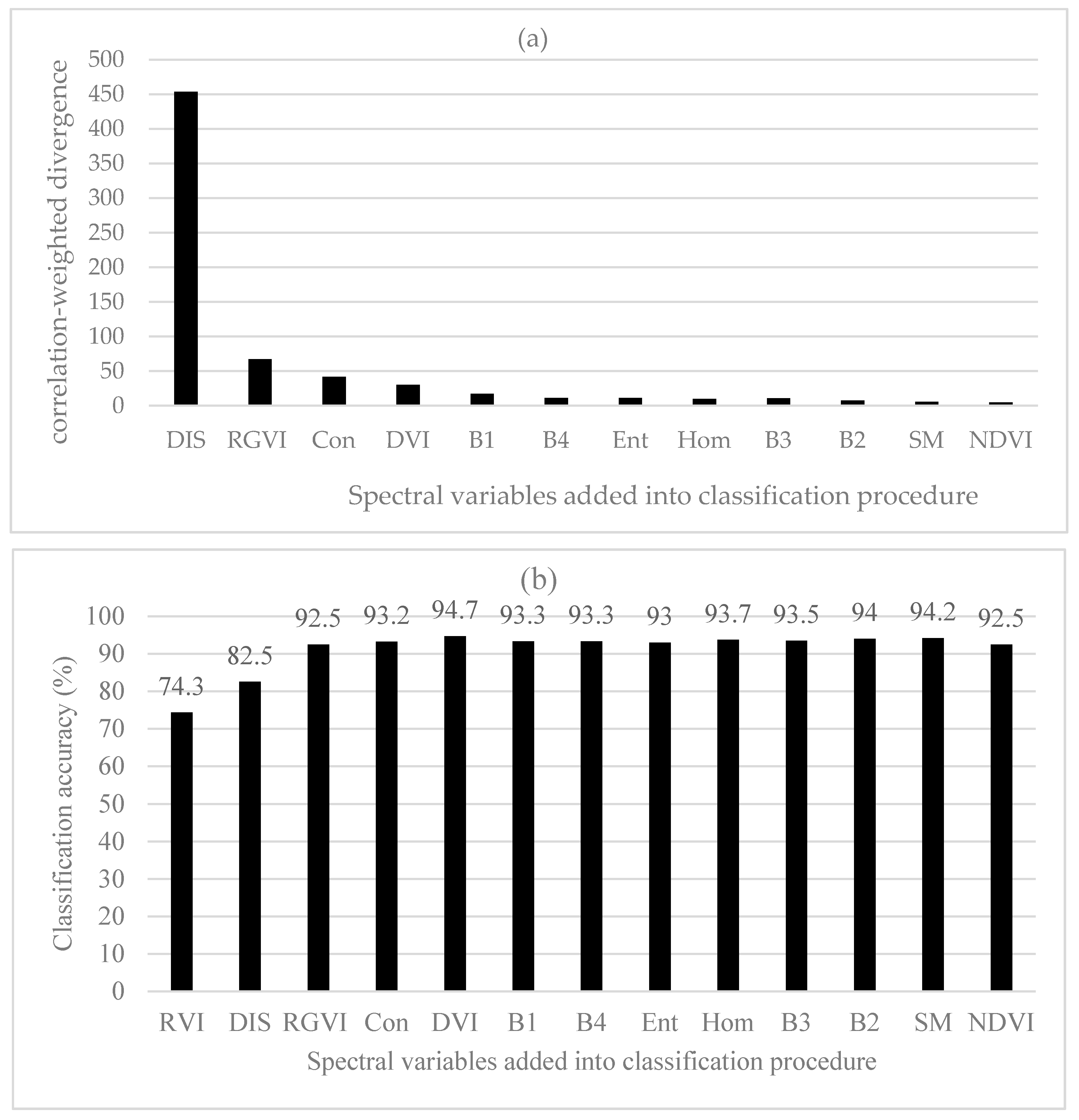
Figure 5a showed the order of the important spectral variables after the first spectral variable RVI and their correlation-weighted divergences. The rank was obtained based on the greatest correlation-weighted divergence value each time for selecting one among the left spectral variables. This rank differed from that using the original divergences without the correlation-weighting. The first spectral variable RVI was chosen based on the divergence values without the variable correlations considered. Compared with other left spectral variables, Dis had the greatest correlation-weighted divergence value and was added as the second spectral variable, then RGVI, Con, DVI, B1, B4, Ent, Hom, B3, B2, SM and NDVI. The use of the first five spectral variables including RVI, DIS, RGVI, Con and DVI led to a largest accuracy of classification (Figure 5b), 94.7%, and the accuracy was slightly greater than the greatest accuracy created by using the first 11 spectral variables based on the original divergences. With the correlation-weighted divergences, the statistically stable classification accuracies started to be produced after the first three spectral variables.
3.2.3. B-Distance and Correlation-Weighted B-Distance
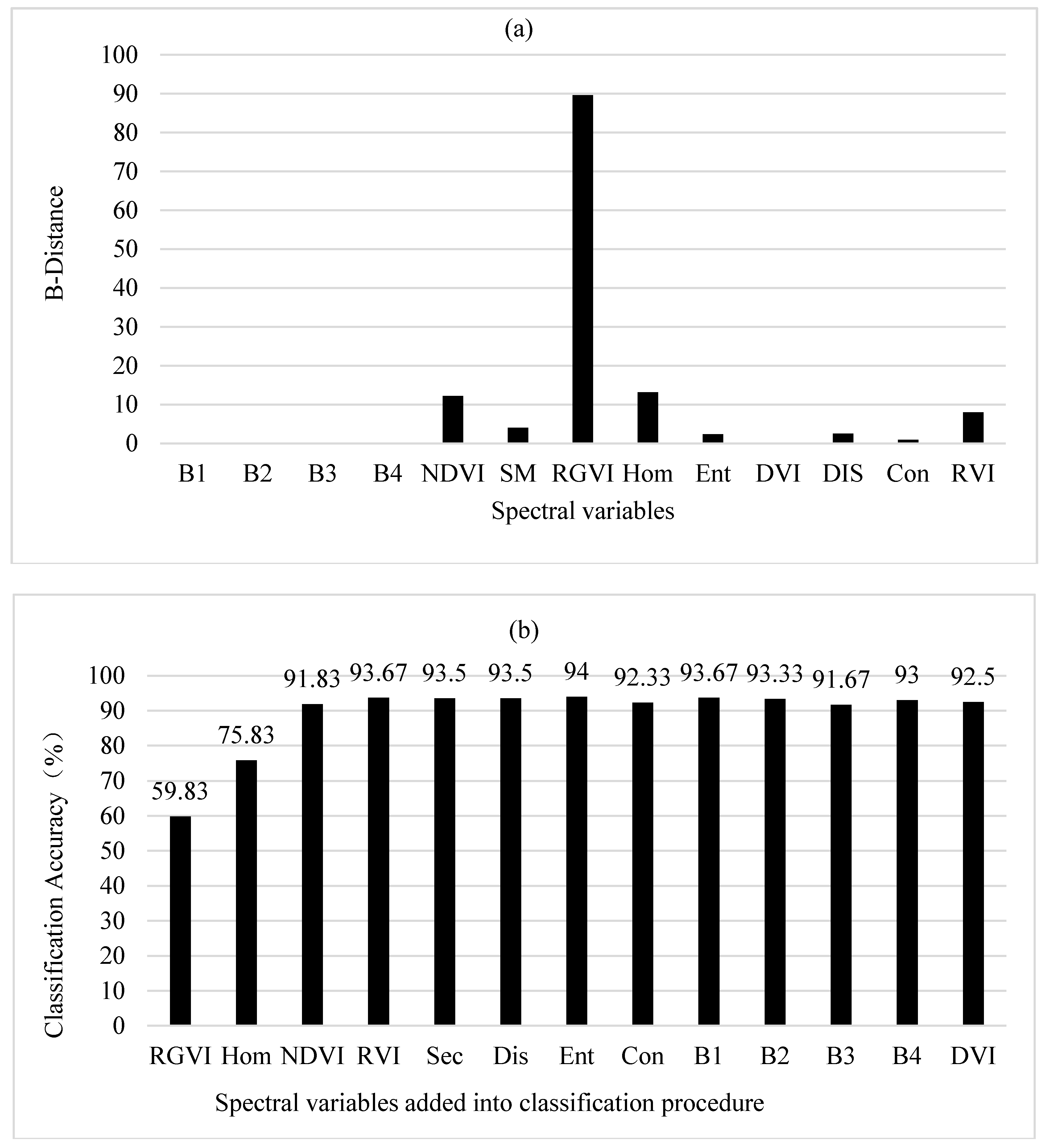
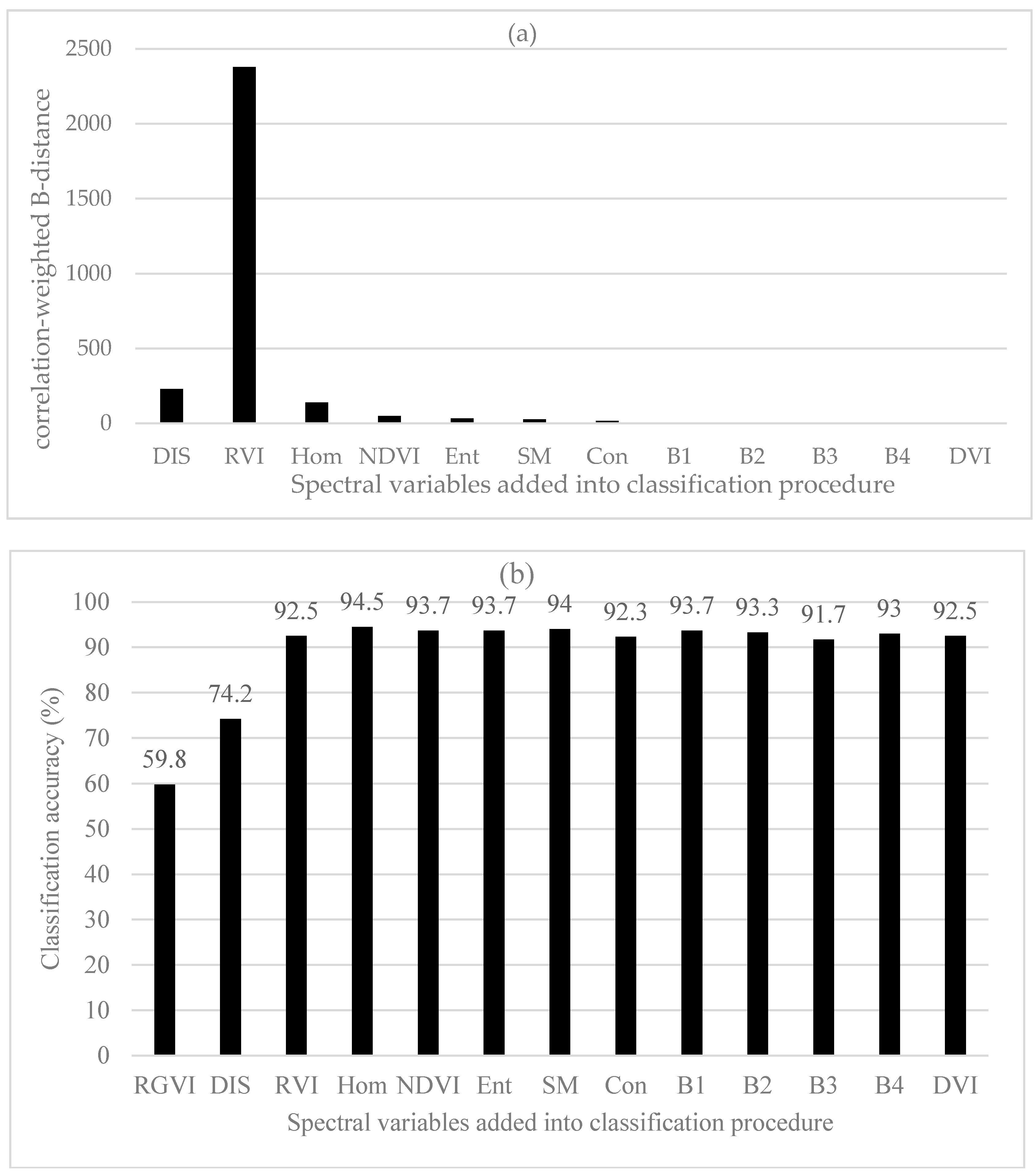
Based on B-distances, the largest value of class separability was achieved by RGVI, then Hom, NDVI, RVI, SM, Dis, Ent, Con, B1, B2, B3, B4 and DVI (Figure 6a). It had to be pointed out that in Figure 6a, the values of B1, B2, B3, B4 and DVI were 0.04, 0.03, 0.01, 0.01 and 0.01, respectively and could not be shown because of being too small. The importance rank of the spectral variables was greatly different from those obtained using the original JM distances and divergences. When the first two spectral variables RGVI and Hom were added, the overall classification accuracies of 59.8% and 75.8% were obtained using BD classifier (Figure 6b). Adding the third spectral variable NDVI led to a great increase of the overall accuracy up to 91.8%. After that, the classification accuracy slightly increased and fluctuated as more spectral variables were introduced. The greatest overall accuracy of 94.0% was yielded when the first seven spectral variables (RGVI, Hom, NDVI, RVI, SM, Dis and Ent) were used. Overall, the statistically stable classification accuracies were found when the number of the selected spectral variables was equal to and greater than 3.
Figure 7a showed the sequentially added spectral variables: DIS, RVI, Hom, NDVI, Ent, SM, Con, B1, B2, B3, B4 and DVI after the first spectral variable RGVI and their correlation-weighted B-distance values. It was noticed that B1, B2, B3, B4 and DVI were not seen in Figure 7a because of too small values (0.39, 0.17, 0.11, 0.09 and 0.08, respectively). Compared with the rank of the important spectral variables obtained based on the original B-distances, the first seven spectral variables were different but the last six spectral variables were same. In Figure 7b, the spectral variables were orderly selected for classification based on the improved class separability quantified by the correlation-weighed B-distances. The first three spectral variables added were RGVI, Dis and RVI, and resulted in the overall classification accuracies of 59.8%, 74.2% and 92.5%, respectively. Introducing the fourth spectral variable Hom led to the largest overall accuracy of 94.5% and after that, adding more spectral variables resulted in slightly fluctuating and slightly lower accuracies. The highest accuracy obtained with the first four spectral variables (RGVI, Dis, RVI and Hom) was slightly greater than the greatest accuracy created by selecting the first seven spectral variables based on the original B-distances and also slightly larger than those with the uses of the original and improved JM distances and divergences. The statistically stable classification accuracies started to be yielded after the first three spectral variables.
3.2.4. Comparison of Methods
Overall, when BD classifier was used for the classification, the original JM distances, divergences and B-distances and the corresponding correlation-weighted measures led to the certain numbers of the selected spectral variables that produced the statistically stable classification accuracies. This indicated that although more spectral variables were added, the obtained classification accuracies statistically did not significantly differ from each other for each of the original and improved class separability measures. It was also found that the statistically stable classification accuracies were not significantly different from each other among all the class separability measures. However, the numbers of the selected spectral variables required to start to achieve the statistically stable classification accuracies were much smaller when the correlation-weighted class separability measures were used than those when the original class separability measures were utilized. This implied that the correlation-weighted class separability measures greatly improved the selection of the spectral variables compared with the original class separability measures.
In order to further validate the improvement of selecting spectral variables for classification based on three correlation-weighted class separability measures, the classification results using BD classifier were compared with those from MD classifier and RF algorithm in Table 2. When MD classifier was used, the uses of more than 4, 3 and 7 spectral variables for the correlation-weighted JM distances, correlation-weighted divergences and correlation-weighted B-distances, respectively, led to non-positive definite matrices. MD classifier requires that the covariance matrix to be analyzed must be positive definite. If the matrix analyzed is not positive definite, the computer program simply gives an error message and quit. Thus, the classification results could not be obtained. However, it was obviously noticed that the obtained classification accuracies had a trend of increase as more spectral variables were introduced at the beginning and seemed to quickly reach their largest values when the first three or four spectral variables were added. The feature was similar to that when BD classifier was utilized but, the former led to slightly larger classification accuracy than the latter.
When RF was used to classify the six land cover types, it was found that the OOB error decreased quickly as the ntree increased from 1 to 10 and then slowly from ntree = 10 to ntree = 100 (The figure was omitted because of limited space). Within the range of ntree = 100 to ntree = 200, the OOB errors were smallest. There was an increase of OOB error at ntree = 200 and after that, the OOB errors became constant. This indicated that the range of ntree = 100 to ntree = 200 was an appropriate interval of classification trees used to obtain a stable classification accuracy. In Table 2, the classification accuracies of RF were obtained using all the sets of the spectral variables selected based on the improved JM distance, divergence and B-distance values. It was noticed that RF created an increased trend of the classification accuracies as the number of the selected spectral variables increased and after the certain numbers of the selected spectral variables, statistically the accuracies were not significantly different from each other given an order of adding the spectral variables. However, the increase of the accuracy was not so quickly as those when MD classifier and BD classifier together with the correlation-weighted class separability measures were employed. Overall, all the statistically stable classification accuracies obtained from the improved class separability measures and three classifiers did not significantly differ from each other. However, the numbers of the selected spectral variables to start to obtain the statistically stable classification accuracies were different among the three classifiers. With MD and BD classifiers, this number was 3 for all three correlation-weighted class separability measures (JM distance, divergence and B-distance), while with RF, this number was 7, 7 and 10 for the same sets of the selected spectral variables based on the correlation-weighted JM distances, divergences and B-distances, respectively. On the other hand, given the same orders of the spectral variables added for the classification, RF needed more spectral variables and time to produce the statistically stable classification accuracies compared with MD and BD classifiers.
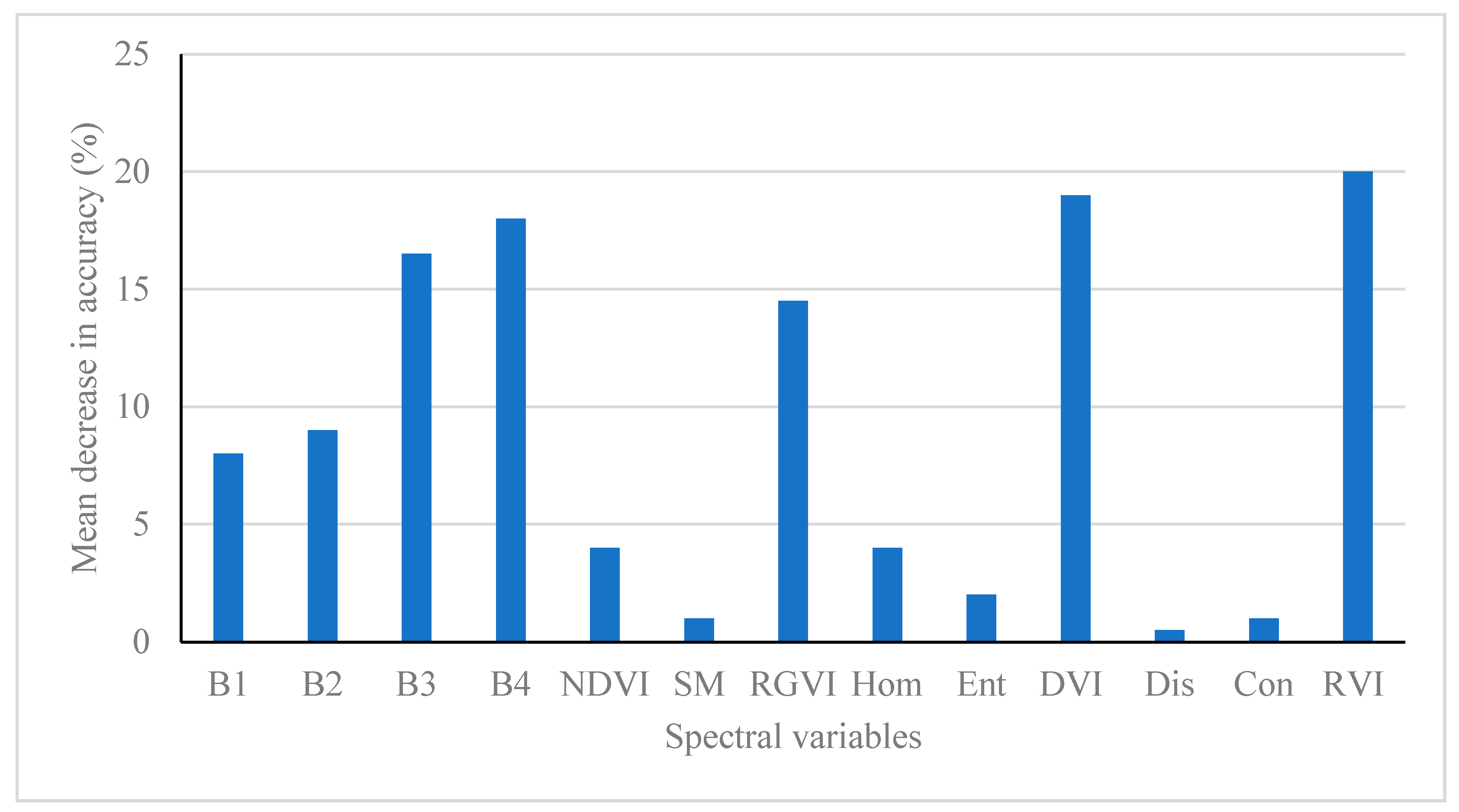
When RF was utilized to optimize the selection of the spectral variables based on the mean decrease in classification accuracy, the obtained rank of the spectral variables from the most important to less important was RVI, DVI, B4, B3, RGVI, B2, B1, NDVI, Hom, Ent, Con, SM and Dis (Figure 8). This importance rank of the spectral variables showed some characteristics that were similar to the ranks from the original JM distances and divergences (Figure 2 and Figure 4). That is, the simpler vegetation indices RVI and DVI and their two relevant original bands B4 and B3, were most important and then the vegetation index RGVI and two original bands B2 and B1. The texture measures had the least importance. The vegetation index NDVI had poorer performance than other three vegetation indices mainly because the division of the differences between B4 and B3 by their sums led to very small values. The importance rank of the spectral variables from RF (Figure 8) was different from the ranks obtained using the correlation-weighted class separability measures (Figure 3, Figure 5 and Figure 7). Using the first 7 most important spectral variables (RVI, DVI, B4, B3, RGVI, B2, B1), RF led to a classification accuracy of 93.5%. The accuracy had no statistically significant differences from the statistically stable classification accuracies by integrating the improved class separability measures with BD and MD classifiers but the number of the used spectral variables by RF was much larger. Removing the significantly correlated spectral variables, RF resulted in an accuracy of 89.5% using 3 most important and un-correlated spectral variables (RVI, B3 and RGVI). This accuracy was significantly smaller than the statistically stable classification accuracies.
Figure 9 compared the land cover classification maps using six methods to select the spectral variables that led to the statistically stable classification accuracies, including the original JM distances, divergences and B-distances and the corresponding correlation-weighted class separability measures. The spatial distributions of six land cover types looked very similar and characterized by the spatial patterns of the water bodies surrounded first by bare lands, then carex areas, reed or phragmites areas and built-up areas. Poplar and willow were scattered in the study area. However, some differences were found at the northeast part of the study area in which using the original JM distance and divergence for the selection of the spectral variables led to more carex area in the phragmites dominant area than using the corresponding correlation-weighted measures. However, the difference was not obvious between the uses of B-distance and correlation-weighted B-distance.
In order to further examine the differences of classification results among the methods, we enlarged the east central part of the study area in Figure 10. It was found there were several big differences of the land cover classification. First of all, when the B-distances with and without correlation-weighting and the correlation-weighted JM distances and correlation-weighted divergences were used for selecting the spectral variables, one rectangle area located in the upper left part of the enlarged region was classified into willow but it was classified into carex by using the original JM distances and divergences. Secondly, the B-distances with and without correlation-weighting and the correlation-weighted JM distances and correlation-weighted divergences led to more willow in one area located in the southwest part of the enlarged region than the original JM distances and divergences. Moreover, one west-east narrow rectangle located in the lower central part of the enlarged region was classified into built-up land by the B-distances with and without correlation-weighting and the correlation-weighted JM distances and correlation-weighted divergences but grouped into carex by the original JM distances and divergences.
As an example, in Table 3 the classification results of six land cover types using the original divergences and correlation-weighted divergences with the same BD classifier were compared. The first four spectral variables were selected for both algorithms of selecting the spectral variables. The numbers of the spectral variables were the same but different spectral variables were obtained. The original divergence led to an overall accuracy of 86.5% with a Kappa value of 0.838 and the correlation-weighted divergence increased the classification accuracy to 93.2% with a Kappa value of 0.918. For the original divergence, the major classification errors occurred among carex, built-up and exposed area and phragmites area and between water bodies and built-up and exposed areas. The producer accuracies for carex, water and built-up and exposed area were 64%, 81% and 76%, respectively. There were 24 and 10 carex plots misclassified into the built-up and exposed area and phragmites area, respectively. There were 20 built-up and exposed area plots incorrectly classified into water bodies. In turn, 19 water plots were misclassified into the built-up and exposed area. The correlation-weighted divergence greatly reduced the misclassifications and increased the producer accuracies of carex and built-up and exposed area to 94% and 89%. However, the correlation-weighted divergence did not improve the classification of water bodies compared with the original divergence.
4. Discussion
When remotely sensed images are used for LULC classification, the accuracy of classification varies greatly depending on selection of spectral variables and improving the selection and combination of the spectral variables is significantly important and very challenging [1,3]. On one hand, there has been a large amount of remotely sensed data available and various vegetation indices, texture measures and image transformations can also be calculated, which lead to the difficulty of selecting spectral variables for classification of LULC types [2,6,37]. On the other hand, the spectral variables may be significantly correlated with each other, which results in the duplication of information [1,6]. Thus, different combinations of spectral variables would produce different classification accuracies. Traditionally, spectral distance-based class separability measures including JM distance, divergence and B-distance have been widely utilized to quantify the importance of spectral variables [1,15]. However, the class separability measures ignore correlations among spectral variables and duplication of information. OIF that is calculated based on both variances of spectral variables and their correlations for each set of spectral variables considers the duplication of information due to the correlations [1]. The larger the OIF value, the greater the potential class separability. However, the values of OIF vary depending on different combinations of spectral variables and the best combination that has the greatest OIF value can be found only after the values of OIF are calculated for all the combinations of spectral variables. This is very time-consuming. RF provides the potential of quantifying the importance of spectral variables for using a great amount of data and a large number of spectral variables [23,24,25,26,27] but still ignores the correlations among spectral variables and duplication of information.
For this purpose, in this study an improved method that takes into account both the class separability and correlations among the used spectral variables was proposed. The proposed method was tested using three widely used class separability measures including JM distance, divergence and B-distance and two parametric classifiers BD and MD and a machine learning algorithm RF to classify six LULC types in the East Dongting Lake, Hunan of China, with a GF-1 image. The results show that all the JM distance, divergence and B-distance methods for selection of spectral variables resulted in the increased classification accuracies with fluctuations as more spectral variables were selected and added into the classification procedure based on the values of the class separability measures from large to small. The number of the selected spectral variables for starting to obtain the statistically stable classification accuracy varied depending on the class separability measures. In order to start to yield the statistically stable classification accuracy, there were 6, 8 and 3 spectral variables needed for the original JM distance, divergence and B-distance, respectively. The duplication of information due to correlations among spectral variables led to the fluctuation of classification accuracy and difficulty to seek the optimal combination of spectral variables for classification.
The proposed method improved the measures of class separability by calculating correlation-weighted JM distances, correlation-weighted divergences and correlation-weighted B-distances. When the improved class separability measures were used together with BD classifier, all the classification accuracies stably and quickly increased as more spectral variables were selected and added and reduced the fluctuations of the classification accuracies. Using the first three spectral variables resulted in the statistically stable classification accuracies for all the improved class separability measures. The finding was also supported by the classification results from MD classifier. This meant that the proposed method led to a solution of selecting the least spectral variables to achieve the statistically stable classification accuracies and increased the effectiveness of selecting the spectral variables. The reason was mainly because the proposed method takes into account the correlations of each variable to be added with the existing spectral variables in the classification procedure. The inverse values of the correlations were used as weights and combined with the values of the class separability measures of this variable to be selected to estimate a potential capacity of classification. The greater the correlation, the smaller the weight and the potential capacity of class separability. Thus, the proposed method reduced the impact of the correlations among spectral variables and is promising for improving the selection of spectral variables.
To further validate the improvement of the proposed method for selection of spectral variables, in this study one advanced machine learning algorithm RF was compared to conduct the classification of six LULC types in addition to two parametric classifiers MD and BD. RF optimizes the classification results [21,22,23] and also ranks the importance of spectral variables [21,22,23,24,25,26,27]. The results of this study showed that integrating MD classifier with the improved class separability measures created the highest classification accuracy, then the combination of BD classifier with the improved class separability measures and RF led to the smallest classification accuracy. Although all the greatest classification accuracies from the methods were not statistically different from each other, RF needed more spectral variables to produce the statistically stable classification accuracies compared with the integrations of the improved class separability measures with MD and BD classifiers. Moreover, RF led to the importance rank of the spectral variables that were overall similar to those from the original class separability measures but different from those using the improved class separability measures. This implied that compared with RF, the proposed method speeded up the selection of the important spectral variables. This was mainly because the proposed method takes into account the correlations among the spectral variables, while RF not. In addition, when the first 7 most important spectral variables were used, RF led to a classification accuracy of 93.5%. The accuracy was similar to the statistically stable classification accuracies achieved by the combinations of the improved class separability measures with MD and BD classifiers but the number of the used spectral variables by RF was much larger than those by the improved class separability measures. When three most important and un-correlated spectral variables were utilized, RF resulted in an accuracy of 89.5% that was statistically significantly smaller than those using the same numbers of the spectral variables selected based on the improved class separability measures. The reason might be because using too few spectral variables in RF reduced the strength of each individual tree in the forest. Finally, RF is a complicated algorithm and often requires a large number of training samples, while the parametric methods are very sensitive to the ratio of the number of the spectral variables to the number of training samples. In this study, a total of 600 training samples and 600 validation samples were used. These sample sizes were relatively large. The conclusions drawn from this study should be thus statistically reliable.
This study area was dominated by water bodies, bare lands and four vegetation types including carex, phragmites or reed, poplar and willow and the vegetation cover types were hardly distinguished due to the wetland environment. In this study, we used a total of thirteen spectral variables and the number of the variables was relatively small. There were several reasons for using the spectral variables. First, the spectral variables represented three groups of widely used remote sensing variables: the original bands, the band 4 (near infrared) relevant vegetation indices and texture measures. Second, the used vegetation indices and texture measures could well account for the characteristics of the bare lands, water bodies and wetland plants in this study area. Third, because of too large images (425,069,096 pixels for each variable or image and total 10.53 GB for the 13 images), the use of more spectral variables would lead to the difficulty of computing. In addition, the objective of this study was to develop and demonstrate an improved class separability-based method to select remote sensing variables derived from images for classification of LULC types. The procedure was generalized and thus, the use of 13 spectral variables did not result in biased conclusions.
In this study, the multi-spectral bands were first sharpened with the panchromatic band, leading to four 2 m spatial resolution bands. The sharpened bands were then scaled up to a 4 m spatial resolution using a window average method. The pan-sharpening enhanced the information of the multi-spectral bands because of higher spatial resolution of the panchromatic band and more details of ground objects. Moreover, several studies have indicated that the window average method is most accurate among the widely used up-scaling methods used to capture the texture characteristics of vegetated areas in the up-scaled images [38,39,40]. In this study, on the other hand, resampling was performed twice on the multi-spectral bands, which changed the values of the image pixels and might have led to uncertainty of classification. Because of limited space and time, the amount of the uncertainty and its impact on the classification accuracy were not discussed in this study. However, based on previous studies [38,39,40], the uncertainty was limited and could be ignored.
Finally, this study focused on the development of the improved method for selection of spectral variables. In addition to three widely used class separability measures, a complicated RF was used for comparison. Thus, the conclusions drawn from this study should be statistically reliable. However, it had to be pointed out that the improved method was only examined using a relatively small number of spectral variables in one study area. In the future studies, further validations of the proposed method are needed by using other class separability measures, more LULC types and spectral variables in other larger and more complicated landscapes.
5. Conclusions
Optimizing selection of spectral variables for LULC classification is still a great challenge although many methods have been developed. In this study, a novel approach was proposed to improve the measure of potential class separability of spectral variables by taking into account correlations among spectral variables. The proposed method was investigated using three class separability measures including JM distance, divergence and B-distance based on 13 spectral variables from a GF-1 image with three classifiers including BD, MD and RF for classification of six LULC types at the East Dongting Lake of Hunan, China. The classification accuracies obtained from the improved class separability measures including correlation-weighted JM distance, correlation-weighted divergence and correlation-weighted B-distance were compared with those from the original class separability measures. The comparisons of the accuracy were also conducted among three classifiers. The results showed that (1) By selecting the first three spectral variables, the proposed approach resulted in the statistically stable classification accuracies for all the improved class separability measures at the significant level of 0.05; (2) The statistically stable classification accuracies obtained by integrating MD and BD classifier with the improved class separability measures were also statistically not significantly different from those by RF; (3) The numbers of the selected spectral variables using the improved class separability measures to create the statistically stable classification accuracies by MD and BD classifiers were much smaller than those from the original class separability measures and RF; and (4) Three original class separability measures and RF led to similar importance ranks of the spectral variables, while the ranks achieved by the improved class separability measures were different. This indicated that the proposed method more effectively and quickly selected the spectral variables to produce the statistically stable classification accuracies compared with the original class separability measures and RF and thus improved the selection of spectral variables for the classification. This method is much simpler than RF and especially promising to improve the selection of spectral variables in the case of hyperspectral images used for classification.
It had to be pointed out that this study focused on the development of the proposed method. Because of the budget and time limitations, the results from the proposed method and its comparisons with other methods were only assessed in one study area. Moreover, only six land cover types were classified using a relatively small number of spectral variables derived from a single fine spatial resolution GF-1 image. In the future study, we will further validate and refine the proposed method using national continuous forest inventory plot data and a large number of spectral variables from various spatial resolution images including Sentinel-2, SPOT, Landsat and Moderate Resolution Imaging Spectroradiometer (MODIS) images for classifying more complicated LULC types for the whole Hunan province of China.
Acknowledgments
This study was partly supported by the National Natural Science Foundation of China “The study on the selection of band windows of forest remote sensing monitoring” (31370639). Wang’s work was supported by the funding from Central South University of Forestry and Technology. The authors also thank the graduate students who participated in the collection of field sample plot data, the editors and reviewers.
Author Contributions
Hui Lin and Guangxing Wang designed the study. Renfei Song carried out the sampling design and data collection. Enping Yan and Renfei Song conducted the preprocessing of remote sensing and plot data. Renfei Song and Hui Lin completed the calculation and wrote the draft of the manuscript. Guangxing Wang wrote and revised the manuscript.
Conflicts of Interest
The authors declare no conflict of interest.
References
- Jensen, J.R. Introductory Digital Image Processing: A Remote Sensing Perspective, 4th ed.; Pearson Prentice Hall: New York, NY, USA, 2016. [Google Scholar]
- Jones, H.G.; Vaughan, R.A. Remote Sensing of Vegetation: Principles, Techniques, and Applications; Oxford University Press, Incorporated: New York, NY, USA, 2010. [Google Scholar]
- Lu, D.; Weng, Q. A survey of image classification methods and techniques for improving classification performance. Int. J. Remote Sens. 2007, 28, 823–870. [Google Scholar] [CrossRef]
- TSO, B.; Mather, P.M. Classification Methods for Remotely Sensed Data; Taylor and Francis Inc.: New York, NY, USA, 2001. [Google Scholar]
- Wang, G.; Weng, Q. Remote Sensing of Natural Resources; CRC Press, Taylor & Francis Group: Boca Raton, FL, USA, 2013. [Google Scholar]
- Haralick, R.M.; Shanmugan, K.; Dinstein, I. Textural features for image classification. IEEE Trans. Syst. Man Cybern. 1973, 3, 610–621. [Google Scholar] [CrossRef]
- Myint, S.W. A robust texture analysis and classification approach for urban land-use and land-cover feature discrimination. Geocarto Int. 2001, 16, 27–38. [Google Scholar] [CrossRef]
- Asner, G.P.; Heidebrecht, K.B. Spectral unmixing of vegetation, soil and dry carbon cover in arid regions: Comparing multispectral and hyperspectral observations. Int. J. Remote Sens. 2002, 23, 3939–3958. [Google Scholar] [CrossRef]
- Landgrebe, D.A. Signal Theory Methods in Multispectral Remote Sensing; John Wiley and Sons: Hoboken, NJ, USA, 2003. [Google Scholar]
- Platt, R.V.; Goetz, A.F.H. A comparison of AVIRIS and Landsat for land use classification at the urban fringe. Photogramm. Eng. Remote Sens. 2004, 70, 813–819. [Google Scholar] [CrossRef]
- Penaloza, M.A.; Welch, R.M. Feature selection for classification of Polar Regions using a fuzzy expert system. Remote Sens. Environ. 1996, 58, 81–100. [Google Scholar] [CrossRef]
- Peddle, D.R.; Ferguson, D.T. Optimisation of multisource data analysis: An example using evidential reasoning for GIS data classification. Comput. Geosci. 2002, 28, 45–52. [Google Scholar] [CrossRef]
- Lhermitte, S.; Verbesselt, J.; Verstraeten, W.W.; Coppin, P. A comparison of time series similarity measures for classification and change detection of ecosystem dynamics. Remote Sens. Environ. 2011, 115, 3129–3152. [Google Scholar] [CrossRef]
- Yan, E.; Wang, G.; Lin, H.; Xia, C.; Sun, H. Phenology-assisted classification of vegetation cover types in Northeast China with MODIS NDVI time series. Int. J. Remote Sens. 2015, 36, 489–512. [Google Scholar] [CrossRef]
- Zheng, Y.K.; Zhuang, D.F. Fourier Analysis of Multi-Temporal AVHRR Data. J. Grad. Sch. Chin. Acad. Sci. 2003, 20, 62–68. [Google Scholar]
- Swain, P.H.; Davis, S.M. Remote Sensing: The Quantitative Approach; McGraw-Hill: New York, NY, USA, 1978. [Google Scholar]
- Thomas, I.L.; Ching, N.P.; Benning, V.M.; D’Aguanno, J.A. A review of multi-channel indices of class separability. Int. J. Remote Sens. 1987, 8, 331–350. [Google Scholar] [CrossRef]
- Ferro, C.J.; Warner, T.A. Scale and texture in digital image classification. Photogramm. Eng. Remote Sens. 2002, 68, 51–63. [Google Scholar]
- Ifarraguerri, A.; Prairie, M.W. Visual Method for Spectral Band Selection. IEEE Geosci. Remote Sens. Lett. 2004, 1, 101–106. [Google Scholar] [CrossRef]
- Dalponte, M.; Bruzzone, L.; Vescovo, L.; Gianelle, D. Role of Spectral Resolution and Classifier Complexity in the Analysis of Hyperspectral Images of Forest Areas. Remote Sens. Environ. 2009, 113, 2345–2355. [Google Scholar] [CrossRef]
- Tin Kam, H. Random Decision Forests. In Proceedings of the 3rd International Conference on Document Analysis and Recognition, Montreal, QC, Canada, 14–16 August 1995; pp. 278–282. [Google Scholar]
- Tin Kam, H. The Random Subspace Method for Constructing Decision Forests. IEEE Trans. Pattern Anal. Mach. Intell. 1998, 20, 832–844. [Google Scholar] [CrossRef]
- Breiman, L. Random Forests. Mach. Learn. 2001, 45, 5–32. [Google Scholar] [CrossRef]
- Hao, P.; Zhan, Y.; Wang, L.; Niu, Z.; Shakir, M. Feature Selection of Time Series MODIS Data for Early Crop Classification Using Random Forest: A Case Study in Kansas, USA. Remote Sens. 2015, 7, 5347–5369. [Google Scholar] [CrossRef]
- Koreen Millard, K.; Richardson, M. On the Importance of Training Data Sample Selection in Random Forest Image Classification: A Case Study in Peatland Ecosystem Mapping. Remote Sens. 2015, 7, 8489–8515. [Google Scholar] [CrossRef]
- Wessels, K.J.; van den Bergh, F.; Roy, D.P.; Salmon, B.P.; Steenkamp, K.C.; MacAlister, B.; Swanepoel, D.; Jewitt, D. Rapid Land Cover Map Updates Using Change Detection and Robust Random Forest Classifiers. Remote Sens. 2016, 8, 888. [Google Scholar] [CrossRef]
- Sharma, R.C.; Tateishi, R.; Hara, K.; Iizuka, K. Production of the Japan 30-m Land Cover Map of 2013–2015 Using a Random Forests-Based Feature Optimization Approach. Remote Sens. 2016, 8, 429. [Google Scholar] [CrossRef]
- Deng, F.; Wang, X.; Li, E.; Cai, X.; Huang, J.; Hu, Y.; Jiang, L. Dynamics of Lake Dongting wetland from 1993 to 2010. Hupo Kexue 2012, 24, 571–576. [Google Scholar]
- Yin, G.Y.; Liu, L.M.; Jiang, X.L. The sustainable arable land use pattern under the tradeoff of agricultural production, economic development, and ecological protection—An analysis of Dongting Lake basin, China. Environ. Sci. Pollut. Res. 2017, 24, 25329–25345. [Google Scholar] [CrossRef] [PubMed]
- Singh, A.; Singh, K.K. Satellite image classification using genetic algorithm trained radial basis function neural network, application to the detection of flooded areas. J. Vis. Commun. Image Represent. 2017, 42, 173–182. [Google Scholar] [CrossRef]
- Ling, C.X.; Ju, H.B.; Zhang, H.Q.; Sun, H. Research on wetland type classification based on improved remote sensing index of worldview-2 data. For. Res. 2014, 27, 639–643. [Google Scholar]
- Hu, J.; Zhang, H.; Ling, C.; Lin, H.; Sun, H.; Wang, G. Wetland information extraction of the East Dongting Lake using mean shift segmentation. In Proceedings of the 3rd International Workshop on Earth Observation and Remote Sensing Applications (EORSA), Changsha, China, 11–14 June 2014. [Google Scholar]
- Thomas, K. The Divergence and Bhattacharyya Distance Measures in Signal Selection. IEEE Trans. Commun. Technol. 1967, 15, 52–60. [Google Scholar]
- Swain, P.H.; King, R.C. Two Effective Feature Selection Criteria for Multispectra Remote Sensing. In Proceedings of the 1st International Joint Conference on Pattern Recognition, Washington, DC, USA, 30 October–1 November 1973; pp. 536–540. [Google Scholar]
- Swain, P.H.; Roberson, T.V.; Wacker, A.G. Comparison of Divergence and B-Distance in Feature Selection; Information Note 020781; Laboratory for Application of Remote Sensing, Purdue University: West Lafayette, IN, USA, 1971. [Google Scholar]
- Mausel, P.W.; Kamber, W.J.; Lee, J.K. Optimum Band Selection for Supervised Classification of Multispectral Data. Photogramm. Eng. Remote Sens. 1990, 6, 55–60. [Google Scholar]
- Jiang, Q.X.; Townshend, J. Texture analysis method is utilized to extract the TM image information. J. Remote Sens. 2004, 5, 458–463. [Google Scholar]
- Hay, G.J.; Niemann, K.O.; Goodenough, D.G. Spatial thresholds, image-objects, and up-scaling: A multi-scale evaluation. Remote Sens. Environ. 1997, 62, 1–19. [Google Scholar] [CrossRef]
- Wang, G.; Gertner, G.Z.; Anderson, A.B. Spatial variability based algorithms for scaling up spatial data and uncertainties. IEEE Trans. Geosci. Remote Sens. 2004, 42, 2004–2015. [Google Scholar] [CrossRef]
- Wang, G.; Gertner, G.Z.; Anderson, A.B. Up-scaling methods based on variability-weighted and simulation for inferring spatial information cross scales. Inter. J. Remote Sens. 2004, 25, 4961–4979. [Google Scholar] [CrossRef]
Figure 1.
The study area–the East Dongting Lake and spatial distribution of sample plots shown in a natural color composite image from Gaofen-1 sensor (right); and its location in China (left).
Figure 1.
The study area–the East Dongting Lake and spatial distribution of sample plots shown in a natural color composite image from Gaofen-1 sensor (right); and its location in China (left).

Figure 2.
(a) Potential class separability of six land cover types for each spectral variable; and (b) the classification accuracies of Bayesian discriminant (BD) classifier as the spectral variables were added based on average Jeffreys–Matusita (JM) distances from large to small.
Figure 2.
(a) Potential class separability of six land cover types for each spectral variable; and (b) the classification accuracies of Bayesian discriminant (BD) classifier as the spectral variables were added based on average Jeffreys–Matusita (JM) distances from large to small.
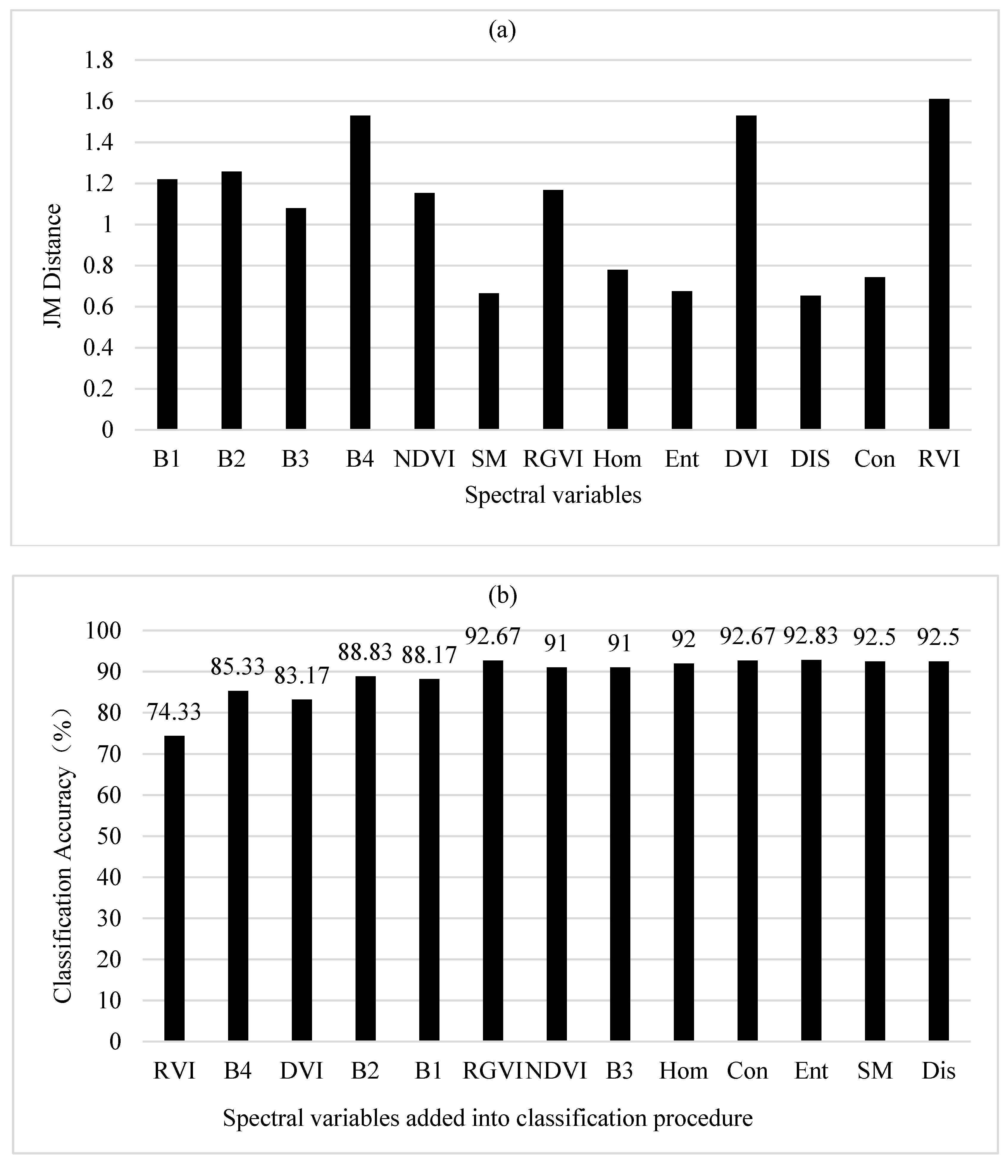
Figure 3.
(a) The correlation-weighted Jeffreys–Matusita (JM) distance of the left 12 spectral variables orderly selected after the first spectral variable RVI; and (b) the classification accuracies of six land cover types using Bayesian discriminant (BD) classifier as the spectral variables orderly added based on the correlation-weighted JM distances.
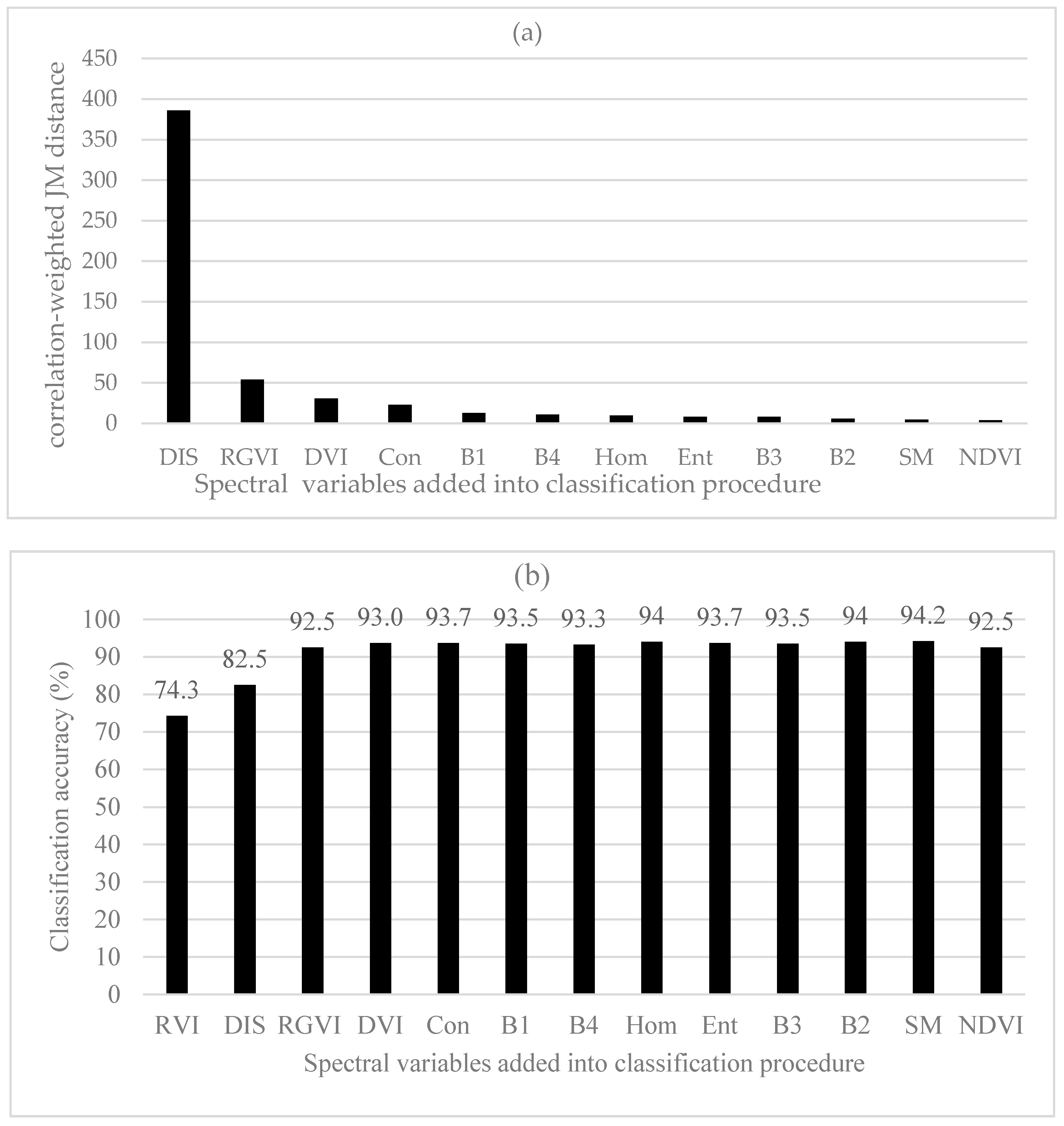
Figure 4.
(a) Potential class separability of six land cover types for each spectral variable; and (b) the classification accuracies of Bayesian discriminant (BD) classifier as the spectral variables were added based on average divergences.
Figure 4.
(a) Potential class separability of six land cover types for each spectral variable; and (b) the classification accuracies of Bayesian discriminant (BD) classifier as the spectral variables were added based on average divergences.
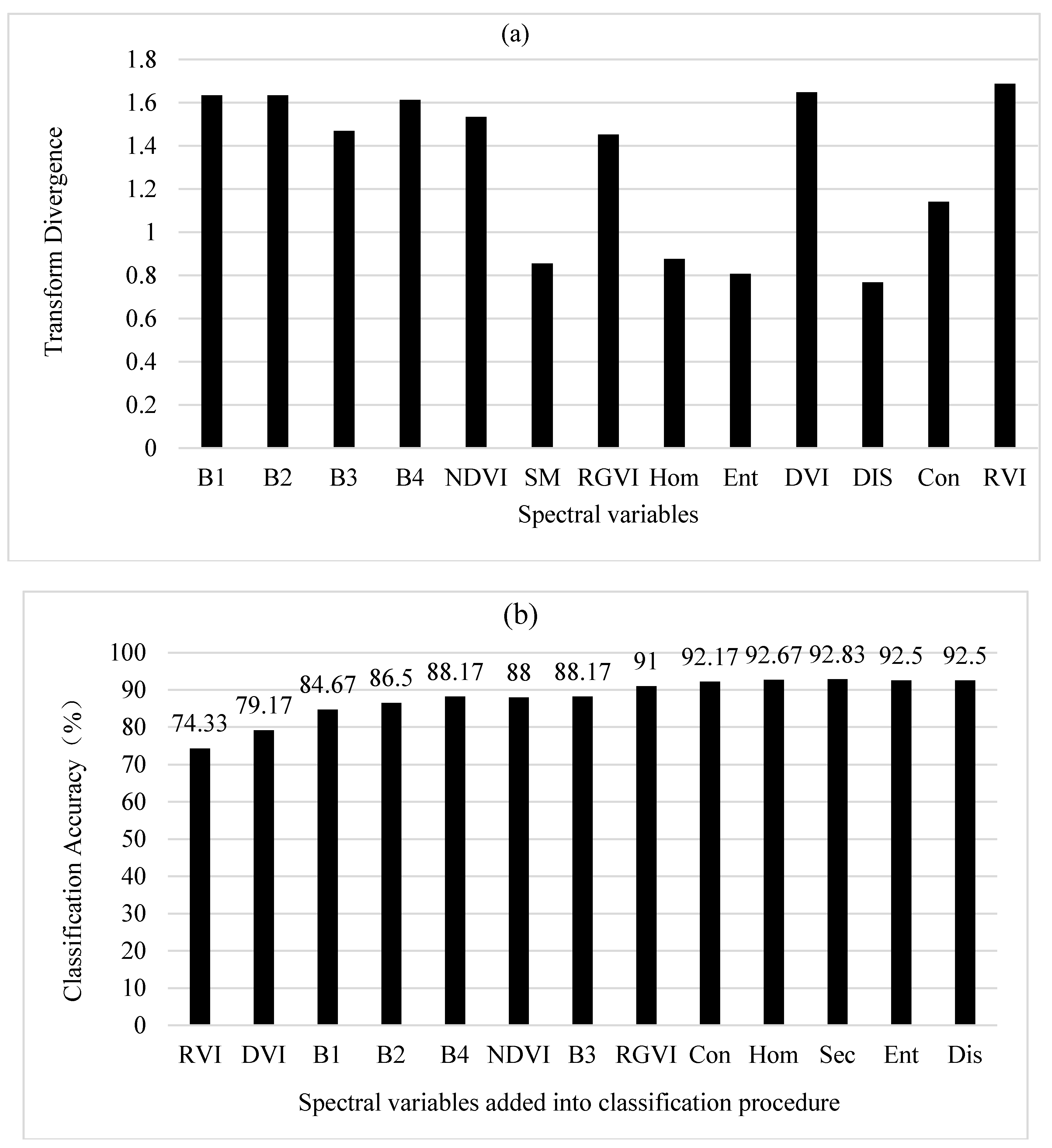
Figure 5.
(a) Correlation-weighted divergences of the left 12 spectral variables selected after the first spectral variable RVI; and (b) the classification accuracies of six land cover types using Bayesian discriminant (BD) classifier as the spectral variables orderly added based on the correlation-weighted divergences.

Figure 6.
(a) Potential class separability of six land cover types for each spectral variable (Note: the values of B1, B2, B3, B4 and DVI were 0.04, 0.03, 0.01, 0.01 and 0.01, respectively and could not be shown because of too small values); and (b) the classification accuracies of Bayesian discriminant (BD) classifier as the spectral variables were added based on average B-distances.

Figure 7.
(a) Correlation-weighted B-distances of the left 12 spectral variables selected after the first spectral variable RGVI (Note: the values of B1, B2, B3, B4 and DVI were 0.39, 0.17, 0.11, 0.09 and 0.08, respectively and could not be shown because of too small values); and (b) the classification accuracies of six land cover types using Bayesian discriminant (BD) classifier as spectral variables were added based on correlation-weighted B-distances.

Figure 8.
The importance of spectral variables quantified using mean decrease in classification accuracy by random forests (RF).
Figure 8.
The importance of spectral variables quantified using mean decrease in classification accuracy by random forests (RF).

Figure 9.
The comparison of land cover type classification maps using six methods to select the first four spectral variables: (a) JM distances; (b) correlation-weighted JM distances; (c) Divergences; (d) correlation-weighted divergences; (e) B-distances and (f) correlation-weighted B-distances.
Figure 9.
The comparison of land cover type classification maps using six methods to select the first four spectral variables: (a) JM distances; (b) correlation-weighted JM distances; (c) Divergences; (d) correlation-weighted divergences; (e) B-distances and (f) correlation-weighted B-distances.
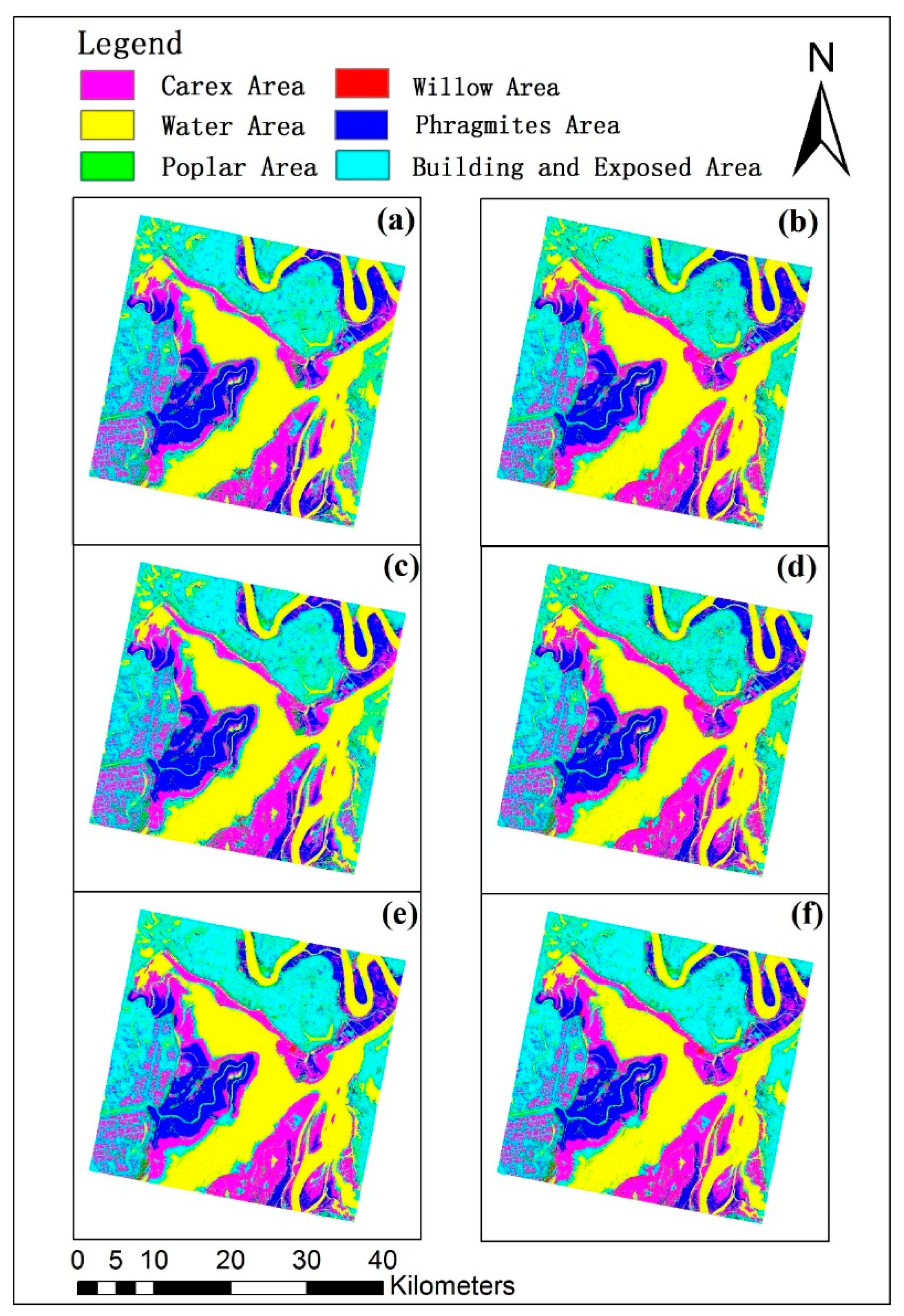
Figure 10.
The comparison of land cover type classification maps for one small region located at the east central part of the study area using six methods to select the first four spectral variables: (a) JM distances; (b) correlation-weighted JM distances; (c) Divergences; (d) correlation-weighted divergences; (e) B-distances and (f) correlation-weighted B-distances.


Table 1.
The Pearson product moment correlation coefficients among 13 spectral variables (note: all coefficients were absolute values).
Table 1.
The Pearson product moment correlation coefficients among 13 spectral variables (note: all coefficients were absolute values).
| B1 | B2 | B3 | B4 | NDVI | RVI | RGVI | DVI | Ent | Hom | Dis | Con | SM | |
|---|---|---|---|---|---|---|---|---|---|---|---|---|---|
| B1 | 1 | 0.9376 | 0.9304 | 0.4281 | 0.5003 | 0.6098 | 0.4527 | 0.5768 | 0.1421 | 0.0672 | 0.0942 | 0.0268 | 0.1408 |
| B2 | 1 | 0.9318 | 0.1851 | 0.3366 | 0.4087 | 0.3280 | 0.3497 | 0.1762 | 0.1131 | 0.1538 | 0.0907 | 0.1560 | |
| B3 | 1 | 0.2481 | 0.3091 | 0.4767 | 0.6400 | 0.4215 | 0.1166 | 0.0470 | 0.1098 | 0.0594 | 0.0947 | ||
| B4 | 1 | 0.8145 | 0.9537 | 0.2909 | 0.9831 | 0.0802 | 0.0480 | 0.0411 | 0.0926 | 0.1414 | |||
| NDVI | 1 | 0.7828 | 0.1368 | 0.8210 | 0.3296 | 0.3258 | 0.2318 | 0.1511 | 0.3577 | ||||
| RVI | 1 | 0.4275 | 0.9829 | 0.1133 | 0.0616 | 0.0017 | 0.0602 | 0.1611 | |||||
| RGVI | 1 | 0.3934 | 0.0177 | 0.0687 | 0.0111 | 0.0108 | 0.0384 | ||||||
| DVI | 1 | 0.0971 | 0.0539 | 0.0177 | 0.0754 | 0.1502 | |||||||
| Ent | 1 | 0.8716 | 0.8885 | 0.7231 | 0.9799 | ||||||||
| Hom | 1 | 0.8918 | 0.7814 | 0.8282 | |||||||||
| Dis | 1 | 0.9286 | 0.8286 | ||||||||||
| Con | 1 | 0.6360 | |||||||||||
| SM | 1 |
Table 2.
Comparison of classification accuracy among three classifiers using the spectral variables selected based on correlation-weighted Jeffreys–Matusita (JM) distances, correlation-weighted divergences and correlation-weighted B-distances (SV: spectral variable; N. of SV: number of spectral variables used; BD: Bayesian discriminant classifier; MD: Mahalanobis distance classifier and RF: random forests; nt: number of trees used in RF).
| N. of SV | Correlation-Weighted JM Distances | Correlation-Weighted Divergences | Correlation-Weighted B-Distances | |||||||||
|---|---|---|---|---|---|---|---|---|---|---|---|---|
| SV | MD | RF (nt = 100) | BD | SV | MD | RF (nt = 100) | BD | SV | MD | RF (nt = 200) | BD | |
| 1 | RVI | 72.8 | 72.2 | 74.3 | RVI | 72.8 | 72.2 | 74.3 | RGVI | 43.0 | 58.5 | 59.8 |
| 2 | DIS | 78.8 | 79.8 | 82.5 | DIS | 78.8 | 79.7 | 82.5 | DIS | 65.0 | 68.8 | 74.2 |
| 3 | RGVI | 94.7 | 88.5 | 92.5 | RGVI | 94.7 | 89.0 | 92.5 | RVI | 94.7 | 88.5 | 92.5 |
| 4 | DVI | 93.0 | 88.2 | 93.0 | Con | 88.7 | 93.2 | Hom | 95.2 | 89.8 | 94.5 | |
| 5 | Con | 88.2 | 93.7 | DVI | 87.2 | 94.7 | NDVI | 93.3 | 89.5 | 93.7 | ||
| 6 | B1 | 88.0 | 93.5 | B1 | 89.8 | 93.5 | Ent | 92.8 | 89.8 | 93.7 | ||
| 7 | B4 | 92.0 | 93.3 | B4 | 92.2 | 93.3 | SM | 92.2 | 89.3 | 94.0 | ||
| 8 | Hom | 93.3 | 94.0 | Ent | 94.0 | 93.0 | Con | 89.5 | 92.3 | |||
| 9 | Ent | 93.3 | 93.7 | Hom | 92.5 | 93.7 | B1 | 90.0 | 93.7 | |||
| 10 | B3 | 93.5 | 93.5 | B3 | 93.5 | 93.5 | B2 | 92.5 | 93.3 | |||
| 11 | B2 | 93.7 | 94.0 | B2 | 93.7 | 94.0 | B3 | 92.8 | 91.7 | |||
| 12 | SM | 94.8 | 94.2 | SM | 93.8 | 94.2 | B4 | 94.0 | 93.0 | |||
| 13 | NDVI | 93.7 | 92.5 | NDVI | 94.3 | 92.5 | DVI | 93.7 | 92.5 | |||
Table 3.
Comparison of classification accuracy using Bayesian discriminant (BD) classifier between the original JM distance and correlation-weighted JM distance (Note: B&E: building and exposed; PA: producer accuracy; UA: user accuracy).
Table 3.
Comparison of classification accuracy using Bayesian discriminant (BD) classifier between the original JM distance and correlation-weighted JM distance (Note: B&E: building and exposed; PA: producer accuracy; UA: user accuracy).
| Land Cover Types | Willow Area | Poplar Area | Phragmites Area | Water Area | Carex Area | B&E Area | Row Total | UA (%) |
|---|---|---|---|---|---|---|---|---|
| Original divergence | ||||||||
| Willow area | 98 | 0 | 0 | 0 | 0 | 3 | 101 | 97.0 |
| Poplar area | 0 | 100 | 0 | 0 | 2 | 0 | 102 | 98.0 |
| Phragmites area | 0 | 0 | 100 | 0 | 10 | 0 | 110 | 90.9 |
| Water area | 0 | 0 | 0 | 81 | 0 | 20 | 101 | 80.2 |
| Carex area | 0 | 0 | 0 | 0 | 64 | 1 | 65 | 98.5 |
| B&E area | 2 | 0 | 0 | 19 | 24 | 76 | 121 | 62.8 |
| Col. total | 100 | 100 | 100 | 100 | 100 | 100 | ||
| PA (%) | 98 | 100 | 100 | 81 | 64 | 76 | ||
| Overall percentage correct: 86.5%, K = 0.838 | ||||||||
| Correlation-weighted divergence | ||||||||
| Willow area | 98 | 1 | 0 | 1 | 1 | 7 | 108 | 90.7 |
| Poplar area | 0 | 99 | 1 | 0 | 1 | 0 | 101 | 98.0 |
| Phragmites area | 0 | 0 | 99 | 0 | 2 | 0 | 101 | 98.0 |
| Water area | 0 | 0 | 0 | 80 | 0 | 3 | 83 | 96.4 |
| Carex area | 2 | 0 | 0 | 1 | 94 | 1 | 98 | 95.9 |
| B&E area | 0 | 0 | 0 | 18 | 2 | 89 | 109 | 81.7 |
| Col. total | 100 | 100 | 100 | 100 | 100 | 100 | ||
| PA (%) | 98 | 99 | 99 | 80 | 94 | 89 | ||
| Overall percentage correct: 93.2%, K = 0.918 | ||||||||
© 2017 by the authors. Licensee MDPI, Basel, Switzerland. This article is an open access article distributed under the terms and conditions of the Creative Commons Attribution (CC BY) license (http://creativecommons.org/licenses/by/4.0/).
Share and Cite
MDPI and ACS Style
Song, R.; Lin, H.; Wang, G.; Yan, E.; Ye, Z. Improving Selection of Spectral Variables for Vegetation Classification of East Dongting Lake, China, Using a Gaofen-1 Image. Remote Sens. 2018, 10, 50. https://doi.org/10.3390/rs10010050
AMA Style
Song R, Lin H, Wang G, Yan E, Ye Z. Improving Selection of Spectral Variables for Vegetation Classification of East Dongting Lake, China, Using a Gaofen-1 Image. Remote Sensing. 2018; 10(1):50. https://doi.org/10.3390/rs10010050
Chicago/Turabian StyleSong, Renfei, Hui Lin, Guangxing Wang, Enping Yan, and Zilin Ye. 2018. "Improving Selection of Spectral Variables for Vegetation Classification of East Dongting Lake, China, Using a Gaofen-1 Image" Remote Sensing 10, no. 1: 50. https://doi.org/10.3390/rs10010050
Note that from the first issue of 2016, this journal uses article numbers instead of page numbers. See further details here.