Article

Comparative Analysis of Chinese HJ-1 CCD, GF-1 WFV and ZY-3 MUX Sensor Data for Leaf Area Index Estimations for Maize

1
State Key Laboratory of Remote Sensing Science, Institute of Remote Sensing and Digital Earth, Chinese Academy of Sciences, Beijing 100101, China
2
College of Resources and Environment, University of Chinese Academy of Sciences, Beijing 100049, China
3
Joint Center for Global Change Studies, Beijing 100875, China
4
Satellite Surveying and Mapping Application Center, National Administration of Surveying Mapping and Geo-Information of China, Beijing 100048, China
*
Authors to whom correspondence should be addressed.
Remote Sens. 2018, 10(1), 68; https://doi.org/10.3390/rs10010068
Submission received: 6 November 2017 / Revised: 25 December 2017 / Accepted: 3 January 2018 / Published: 5 January 2018

Abstract

:
In recent years, China has developed and launched several satellites with high spatial resolutions, such as the resources satellite No. 3 (ZY-3) with a multi-spectral camera (MUX) and 5.8 m spatial resolution, the satellite GaoFen No. 1 (GF-1) with a wide field of view (WFV) camera and 16 m spatial resolution, and the environment satellite (HJ-1A/B) with a charge-coupled device (CCD) sensor and 30 m spatial resolution. First, to analyze the potential application of ZY-3 MUX, GF-1 WFV, and HJ-1 CCD to extract the leaf area index (LAI) at the regional scale, this study estimated LAI from the relationships between physical model-based spectral vegetation indices (SVIs) and LAI values that were generated from look-up tables (LUTs), simulated from the combination of the PROSPECT-5B leaf model and the scattering by arbitrarily inclined leaves with the hot-spot effect (SAILH) canopy reflectance model. Second, to assess the surface reflectance quality of these sensors after data preprocessing, the well-processed surface reflectance products of the Landsat-8 operational land imager (OLI) sensor with a convincing data quality were used to compare the performances of ZY-3 MUX, GF-1 WFV, and HJ-1 CCD sensors both in theory and reality. Apart from several reflectance fluctuations, the reflectance trends were coincident, and the reflectance values of the red and near-infrared (NIR) bands were comparable among these sensors. Finally, to analyze the accuracy of the LAI estimated from ZY-3 MUX, GF-1 WFV, and HJ-1 CCD, the LAI estimations from these sensors were validated based on LAI field measurements in Huailai, Hebei Province, China. The results showed that the performance of the LAI that was inversed from ZY-3 MUX was better than that from GF-1 WFV, and HJ-1 CCD, both of which tended to be systematically underestimated. In addition, the value ranges and accuracies of the LAI inversions both decreased with decreasing spatial resolution.

Graphical Abstract

1. Introduction

Leaf area index (LAI) is defined as one-half the total foliage area per unit ground surface area [1], and it is an important parameter for monitoring vegetation growth conditions [2,3]. LAI is a common variable that is used for regional and global climate, ecological, and hydrological models [4,5]. LAI has been widely used in global primary productivity measurements [6], agricultural yield estimations [7,8], and ecological and environmental assessments [9]. High-spatial-resolution LAI products play important roles in monitoring regional vegetation changes and evaluating the accuracy of low- resolution LAI products [10,11,12].
From the Landsat-5 satellite launched in 1984 to the present, there are many moderate- to high-resolution satellite sensors that are available in the world, such as the Landsat thematic mapper (TM)/enhanced thematic mapper plus (ETM+)/operational land imager (OLI), Terra advanced spaceborne thermal emission and reflection radiometer (ASTER), SPOT high resolution geometrical (HRG), IKONOS multi-spectral (MS), Sentinel-2 multispectral imager (MSI), and the Chinese environment satellite (HJ-1) charge coupled device (CCD), etc. Generally, LAI extracted from this moderate- to high-resolution imagery largely depends on the empirical relationships. Empirical expressions were established between LAI field measurements and the spectral vegetation indices (SVIs) from isolated dates [13,14,15,16,17,18,19]. The most commonly used SVIs include the normalized difference vegetation index (NDVI), the simple ratio index (SR), and the enhanced vegetation index (EVI) [14,15,20,21,22,23]. In addition, the reduced simple ratio (RSR), the soil-adjusted vegetation index (SAVI), and the perpendicular vegetation index (PVI) are widely used for LAI extraction [21,24,25,26]. When compared with LAI field measurements, the accuracies of satellite LAI estimates based on linear and non-linear regressions of the SVI-LAI relationships have coefficient of determination (R2) values from approximately 0.37 to 0.98 and root mean square error (RMSE) values from approximately 0.17 m2/m2 to 1.14 m2/m2 for both crops (e.g., winter wheat, maize, and soybean) and forests (e.g., coniferous and deciduous) [16,21,23,27,28]. In addition, the SVI-LAI relationships are stronger for crop canopies than for coniferous forests, and are weakest for deciduous forests [15,22,29]. Empirical methods are computationally efficient when using remote sensing datasets at regional or large scales. However, empirical relationships that typically depend on unique vegetation types and regions are often constructed and used locally.
The physical model method, which is suitable for a variety of vegetation types, is also used to extract LAI from moderate- to high-resolution imagery [30,31,32,33,34,35,36,37]. Canopy reflectance models simulate the physical relationship between the canopy reflectance and the LAI in the forward direction. The scattering by arbitrarily inclined leaves with the hot-spot effect (SAILH) model [30,32,38], the Markov chain reflectance model (MCRM) [31], and the Li-Strahler geometric-optical model [34] have been used to extract LAI from moderate- to high-resolution imagery. LAI has also been estimated by indirect methods based on the inversion of canopy reflectance models, such as look-up tables (LUTs) and hybrid methods. The hybrid methods include decision tree learning, artificial neural networks, kernel methods, and Bayesian networks [39]. Additionally, the currently used indirect methods of the radiative transfer model (RTM) for Landsat ETM+ and Sentinel-2 MSI data are the LUT and neural networks [31,32,35,36]. The accuracy of satellite LAI inversions is better than SVI-LAI empirical relationships, with R2 values from 0.54 to 0.82 and RMSE values from 0.17 m2/m2 to 0.71 m2/m2 for crops (e.g., maize and soybean), shrubs, and planted forests [30,31,33,34].
LAI field measurements were acquired via direct and indirect methods [40]. Direct LAI measurements, including leaf collection from deciduous forests and the destructive sampling of crops or low shrubs, are time consuming and difficult to collect at larger areas [40]. Indirect LAI measurement, including optical sensor-based method (such as those using the Licor LAI-2200 Plant Canopy Analyzer (LI-COR, Lincoln, NE, USA) [41], Tracing Radiation and Architecture of Canopies (TRAC) (3rd Wave, Nepean, ON, Canada) [42], AccuPar (Decagon Devices, Inc., Pullman, WA, USA) [43]), digital hemispherical photography (DHP), and new smartphone camera sensor technology (such as LAISmart [44,45] and PocketLAI [46]). These indirect methods are generally convenient, especially those that allow for LAI estimation using a smartphone, and generally efficient over larger spatial scales.
In recent years, China has developed and launched several satellites, such as the HJ-1A/B with a CCD sensor, the GaoFen No. 1 satellite (GF-1) with a wide field of view (WFV) camera and the resources satellite No. 3 (ZY-3) with a multi-spectral camera (MUX). Currently, the satellite data of ZY-3 MUX, GF-1 WFV, and HJ-1 CCD have been applied for vegetation monitoring. HJ-1 CCD data have been widely used for LAI extraction at the regional scale based on SVI-LAI relationships or physical models [21,30,33,34,47]. In addition, GF-1 WFV data have been used to extract the fractional vegetation cover (FVC) [48,49] and estimate LAI from the NDVI-LAI empirical relationship [21,50,51] at the regional scale. However, there have not been any studies that have reported the extraction of LAI from ZY-3 MUX data. One of the objectives of this study is to analyze the potential use of three Chinese satellites, especially ZY-3 MUX, to extract LAI at the regional scale.
The study area was selected in the Huailai experiment station, Hebei Province, China. The satellite data from ZY-3 MUX, GF-1 WFV, and HJ-1 CCD for the study area were collected close to the date of LAI field measurements. The LAI extraction method was a physical model-based SVI- LAI relationship that was generated from the LUT based on the PROSPECT-5B + SAILH (PROSAIL) model with specific input parameters for each sensor (Section 2). In order to assess the surface reflectance quality of ZY-3 MUX, GF-1 WFV, and HJ-1 CCD after data preprocessing, the well- processed surface reflectance products of Landsat-8 OLI with a convincing data quality are used to compare the performances of these sensors, both in theory and reality. Furthermore, the accuracy of the LAI estimation results from ZY-3 MUX, GF-1 WFV, and HJ-1 CCD was validated based on LAI field measurements from the Huailai experiment station (Section 3). The up-scaled LAI inversions for ZY-3 MUX and GF-1 WFV were also compared with the HJ-1 CCD data at the same spatial resolutions for pure and mixed pixels (Section 3). The discussion and conclusions are presented in Section 4 and Section 5, respectively.

2. Materials and Methods

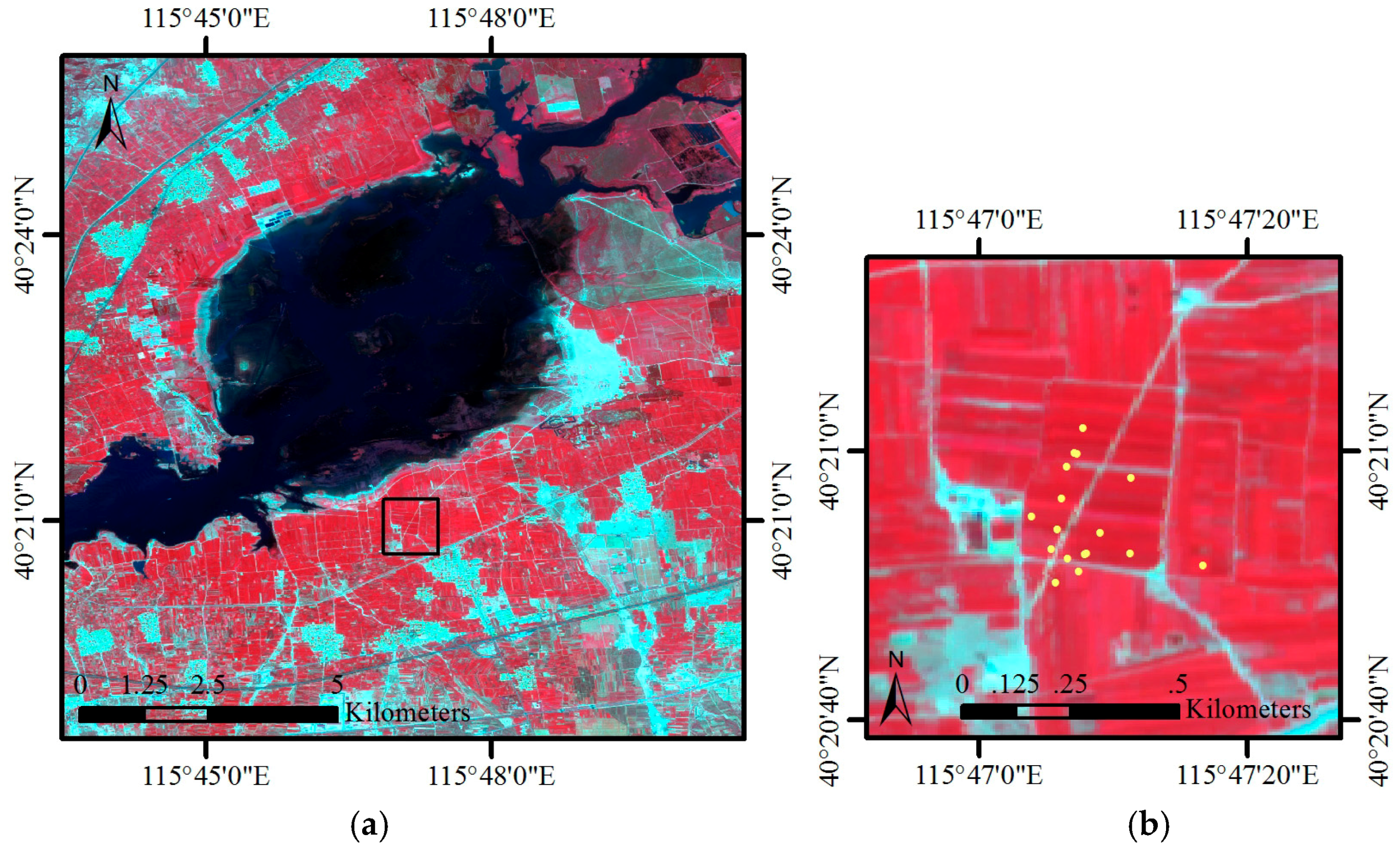
2.1. Study Area and Field Measurements

The study area was at the Huailai experimental field (40°20′55.093″N, 115°46′59.569″E, altitude 488 m) in Hebei Province, China. This field is affiliated with the Chinese Academy of Sciences (CAS) (Figure 1). The study area is in a temperate and semi-arid region with four distinct seasons, abundant sunshine, simultaneous heat and moisture, and large temperature differences. The annual average temperature and average precipitation are approximately 9.5 °C and 392 mm, respectively. The primary vegetation type around the Huailai experimental field is farmland, and other land cover types are water, wetland beach, and residential. Maize is the dominant crop type in this study area. The soil type of the study area is brown soil.
Several vegetation structure parameters (e.g., leaf reflectance and transmittance, average leaf angle, canopy spectral measurements, and LAI) and biophysical and biochemical parameters (e.g., leaf chlorophyll-a and -b content (Cab), leaf water content (Cw), and leaf dry matter content (Cm)) were acquired at the Huailai experimental field. The leaf reflectance and transmittance from 400 nm to 2500 nm were measured using a UV molecular spectroscopy (Lambda 900, PerkinElmer Inc., Waltham, MA, USA). The leaf inclination angle was the angle between a leaf and its normal direction, and was measured using a protractor. The average leaf angle is the mean leaf inclination angle for an entire plant. The canopy and soil spectra were measured using a spectroradiometer (Analytical Spectral Devices, ASD, Longmont, CO, USA) covering wavelengths from 400 nm to 1100 nm with a 5° field of view at noon on sunny days. Cab was based on an average of six points on each leaf three times using the SPAD 502DL plus Chlorophyll meter (Spectrum technologies, Inc., Bridgend, UK). The fresh leaves were weighed and placed into an envelope bag. The envelope bag was then put in the oven at 105 °C for 30 min and then at 85 °C for 24 h. Cm is the weight of leaves after oven drying, and Cw is the proportion of leaf water (fresh weight minus dry weight) to the dry weight.
In this study, LAI field measurements from maize sample plots were acquired on 31 July 2014 (yellow dots in Figure 1b). The sample plots were selected based on NDVI values from Landsat-8 OLI according to Zeng et al. [52]. Then, the sample plots were selected in the field with a single plant type and uniform growth base on the coordinates from global positioning system (GPS). Finally, 17 sample plots were acquired in the study area. LAI field measurements were acquired using an LAI-2200 Plant Canopy Analyzer (LI-COR, Inc., Lincoln, NE, USA). The LAI of each sample plot was measured from one above-canopy reading and nine below-canopy readings with a 45° view cup. The measurements were obtained from 06:30 to 10:00 and from 16:30 to 19:30 to avoid measurement errors caused by the direct sunlight, and the LAI value was measured twice at each site. To reduce the observer effects and other sources of error during LAI field measurements, except for the records of the fifth view angle (centered at 68°) acquired from the LAI-2200 instrument, all of the LAI field measurements were calculated based on a standard error LAI (SEL) of less than 0.5.

2.2. Remote Sensing Data and Preprocessing

The HJ-1 satellite was launched on 6 September 2008, and the ZY-3 satellite was launched on 9 January 2012. Both the HJ-1 satellite and the ZY-3 satellite were launched from the Taiyuan Satellite Launch Center, Shanxi Province, China. The GF-1 satellite was launched on 26 April 2013 from the Jiuquan Satellite Launch Center, Gansu Province, China. The HJ-1, GF-1 and ZY-3 satellites are in sun synchronous orbits at altitudes of 649 km, 645 km, and 505 km, respectively. The technical specifications for the ZY-3 MUX, GF-1 WFV, and HJ-1 CCD sensors are shown in Table 1. Four spectral channels that are distributed in the visible and near-infrared (NIR) spectral domain ranging from 450 nm to 900 nm are identical in these three sensors. The radiometric resolutions of the GF-1 WFV and ZY-3 MUX sensors are higher than that of HJ-1 CCD by 2 bits, which improves the detectability of changes in the feature characteristics. The HJ-1 CCD data have a spatial resolution of 30 m, and the revisit time is approximately four days over China due to the combination of two satellites (HJ-1A and HJ-1B) with two cameras (CCD1 and CCD2) on each satellite. The GF-1 WFV data have a spatial resolution of 16 m and a revisit time of four days among the four combined cameras. The ZY-3 MUX data have the highest spatial resolution of 5.8 m, but the 51 km swath width is much narrower than that of the other two cameras.

2.2.1. Remote Sensing Data Acquisition

The ZY-3 MUX data were acquired from the Satellite Surveying and Mapping Application Center (SASMAC) of the National Administration of Surveying, Mapping and Geo-information of China (NASG) [53]. The GF-1 WFV data were acquired from the Gaofen satellite data and information service system (GFDIS) [54], and the HJ-1 CCD data were acquired from the China Centre for Resources Satellite Data and Application (CRESDA) [55]. The surface reflectance data of Landsat-8 OLI for the study area was acquired from the United States Geological Survey (USGS) [56]. The Landsat-8 OLI data was used to evaluate the data stability of different sensors among ZY-3 MUX, GF-1 WFV and HJ-1 CCD. The acquisition information for these satellite data sources is provided in Table 2. All of the images over the study area were cloudless.

2.2.2. Remote Sensing Data Preprocessing

Preprocessing of the remote sensing data included radiometric calibration, geometric correction, and atmospheric correction. First, radiometric calibration converted the digital number value of the raw image to radiance based on Equation (1) [55].
L e ( λ e ) = G a i n D N + O f f s e t
where L e ( λ e ) is the radiance, and Gain and Offset are the calibration coefficients. The unit is W × m 2 × s r 1 × μ m 1 The Gain and Offset values for ZY-3 MUX, GF-1 WFV, and HJ-1 CCD were obtained from the CRESDA and are shown in Table 3 [55].
However, due to the unstable radiation performance of HJ-1 CCD data, a cross-radiometric calibration was conducted using a method that considers the characteristics of the surface bidirectional reflectance distribution function (BRDF) [47,57]. The calibration accuracy of the four spectral bands of the HJ-1 CCD sensor was 5%, which meets the requirements for absolute radiometric calibration accuracy [58].
The radiance was then converted to top of atmosphere (TOA) reflectance based on Equation (2) [16].
ρ = π L d 2 E S U N λ cos θ s
where ρ is TOA reflectance, π is 3.1415, L is the sensor spectral radiance, d is the earth-sun distance in astronomical units, E S U N λ is the extraterrestrial solar irradiance, and θ s is the solar zenith angle. The E S U N λ values for ZY-3 MUX, GF-1 WFV, and HJ-1 CCD are shown in Table 3 [55].
Because of the high quality of the raw ZY-3 MUX and GF-1 WFV data on clear days, the atmospheric correction of these images was conducted using FLAASH in Environment and Visualizing Images (ENVI) software. However, due to the unstable data quality of HJ-1 CCD, the cross-radiometric calibration and atmospheric correction were accomplished simultaneous using the method proposed by Zhong et al. [57,59]. The atmospheric correction for the HJ-1 CCD image was conducted using a space-based aerosol optical depth (AOD) retrieval method [59]. The differences between the AOD retrieved from the HJ-1 CCD data and that from the Aerosol Robotic Network (AERONET) measurements ranged from –0.14 to 0.31. Approximately 50% of the derived AOD values correlated with AERONET AOD values with low discrepancy (less than 0.15), and the RMSE values for Xianghe and Beijing were 0.18 and 0.21, respectively.
The ZY-3 MUX image was corrected by its own coordinate file (*.rpc) that was acquired from NASG [53]. The geometric corrections of the HJ-1 CCD and GF-1 WFV images were conducted in ENVI software using the geometric correction image of ZY-3 MUX as the reference, and a second- order polynomial transformation with bilinear interpolation was used in the resampling. There were approximately 20 control points that were manually selected from the images, and the geometric registration error was less than one pixel of the images. The remote sensing data for the selected study area were projected to the World Geodetic System of 84 (WGS-84).

2.3. Generating the Forward Simulations

The widely used turbid medium model, i.e., SAILH, which is corrected by the hot-spot parameter, was selected due to its ease of use and consistent performance in validation practices [60,61]. The input parameters in the SAILH model included LAI, average leaf inclination angle (ALA), hot-spot, soil reflectance, leaf reflectance, leaf transmittance, diffuse fraction, solar zenith angle (SZA), view zenith angle (VZA), and relative azimuth angle (RAA). The leaf reflectance and transmittance values were simulated by the PROSPECT-5B model using several biochemical and biophysical parameters, including leaf mesophyll structure (N), Cab, Cm, Cw, carotenoid content (Car), and brown pigment content (Cbrown) [62]. The PROSPECT-5B+SAILH (PROSAIL) model has been used for more than twenty years for the retrieval of vegetation biophysical properties [63,64]. Previous studies have demonstrated that LAI, ALA, and Cab have significant influences on canopy reflectance in the visible and NIR bands. However, other parameters, e.g., N, Cm, and Cw, are less sensitive to the canopy reflectance corresponding to the satellite bands [63,65]. Therefore, the parameters, e.g., N, Cm, Cw Car, and Cbrown, in the PROSAIL model were fixed during the simulation to reduce the complexity and improve the efficiency of the LAI inversion. In this study, the soil reflectance for the PROSAIL model was acquired from field measurements. The parameters for maize, e.g., N, Cm, Cw Car, and Cbrown, were fixed according to LOPEX’93. ALA varied from 40° to 70° at intervals of 10°; Cab varied from 40 to 60 at intervals of 10; SZA varied from 0° to 85° at intervals of 1°; VZA varied from 0° to 35° at intervals of 1°; and, LAI varied from 0 to 8 at intervals of 0.1 (Table 4).
The PROSAIL model was then run to simulate the actual satellite observations of canopy reflectance based on the spectral response curves of ZY-3 MUX, GF-1 WFV, and HJ-1 CCD, which were acquired from CRESDA [55], and of Landsat-8 OLI, which was acquired from USGS [56] (Figure 2). The reflectance simulations of each band based on each satellite spectral response can be calculated from Equation (3) [16].
ρ s ( λ ) = λ min λ max ρ s ( λ i ) φ ( λ i ) d λ λ min λ max φ ( λ i ) d λ
where ρ s ( λ ) is the simulated band reflectance of the satellite sensor, λ min and λ max are the lower and upper band wavelength limits, ρ s ( λ i ) is the simulated hyperspectral reflectance for the ith wavelength, and φ ( λ i ) is the spectral response coefficient of the different sensors for the ith wavelength.

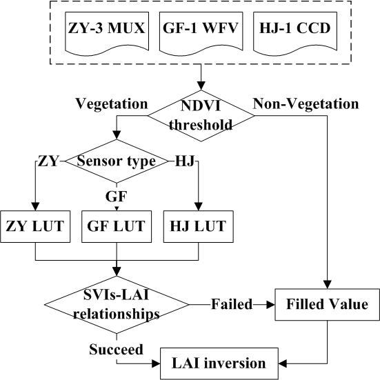
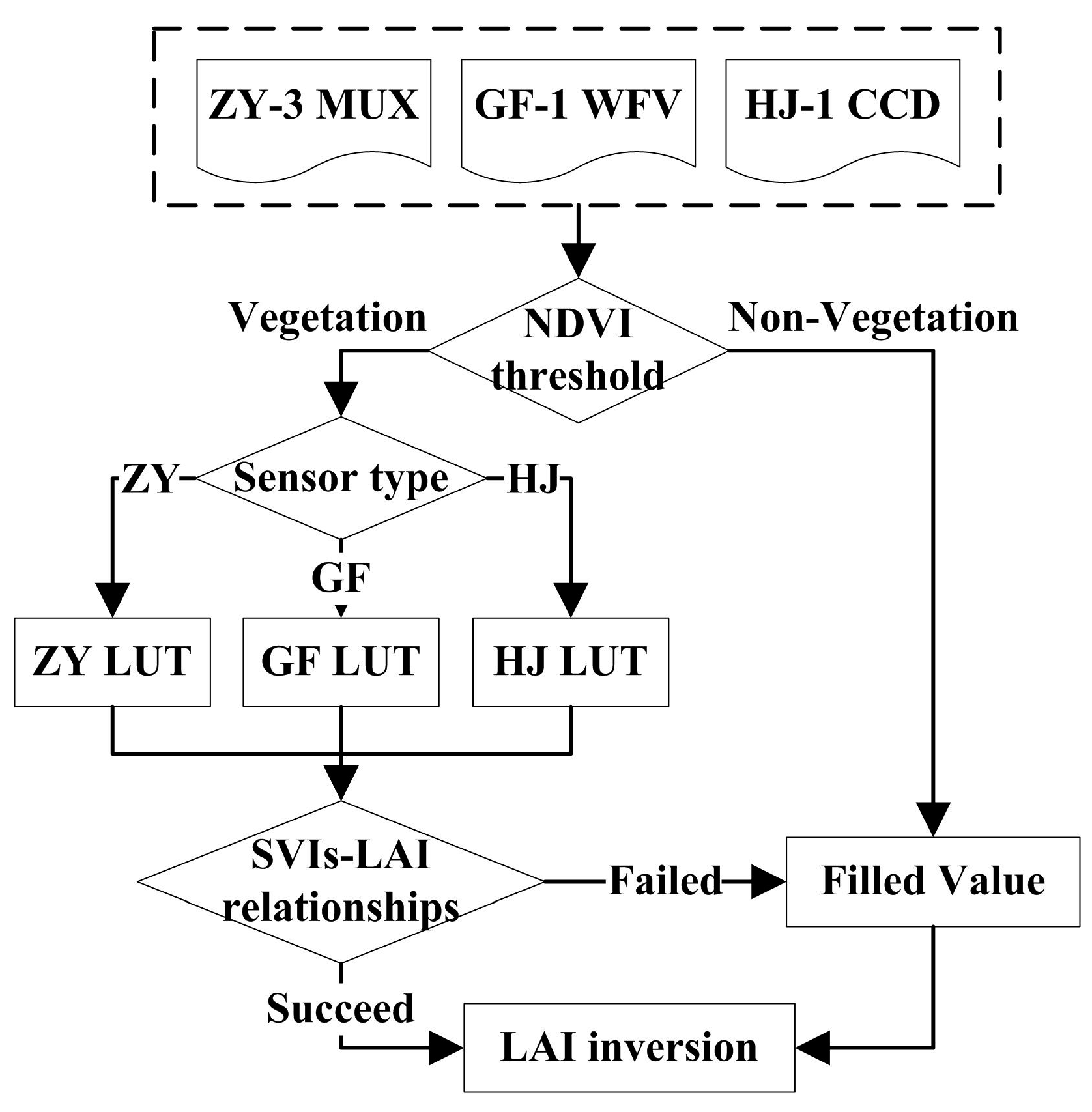
2.4. LAI Inversion Procedures

Before implementing the LAI inversion, the NDVI was used to separate the vegetation and non-vegetation pixels, and the non-vegetation pixels were removed. Generally, the NDVI values were less than 0.05 for bare soil [66,67]. Therefore, the pixels with NDVI values of less than 0.05 were identified as non-vegetation and were set to a filled value (marked as 0).
The LAI inversion method was chosen from the SVI-LAI empirical relationship based on the PROSAIL physical model to reduce the influences from the differences between the various sensors and spectral response curves and the residual errors from data preprocessing. The selected SVIs of this study include the NDVI and an NDVI combined with the NIR reflectance of vegetation (NIRv). The NDVI is a key parameter that is used to improve the accuracy of yield prediction for sugar beets, spring wheat, corn, and sunflower based on the NDVI relationships with optical signals under different nitrogen (N) and sulfur (S) contents [68,69,70,71,72,73,74,75,76]. Notably, the NDVI has been widely used for LAI extraction from high spatial resolution imagery [21,22,24,25,29,77]. NIRv is a new index that directly reflects the proportion of photons intercepted by chlorophyll, and it has a stronger linear relationship with LAI than does the NDVI [78].
Based on the simulation input parameters in Table 4, there are 2,972,160 records in the LUTs for each sensor. During the process of LAI inversion, the specific relationship between SVI and LAI was established according to the values of VZA and SZA for each sensor. Under the illumination and observation conditions of each sensor in the study area, the specific NDVI-LAI and NIRv-LAI exponential relationships for ZY-3 MUX, GF-1 WFV, and HJ-1 CCD were established from the PROSAIL LUT simulations for each sensor (details shown in Table 5). The NDVI and NIRv both had strong relationships with the LAI, and the R2 values for ZY-3 MUX, GF-1 WFV, and HJ-1 CCD were all higher than 0.91. Moreover, all of the R2 values for the NIRv-LAI exponential relationship were higher than those of the NDVI-LAI exponential relationship. LAI estimated from the specific NDVI-LAI and NIRv-LAI exponential relationships based on the image NDVI and NIRv calculations for ZY-3 MUX, GF-1 WFV, and HJ-1 CCD. The flowchart of the LAI inversion method based on ZY-3 MUX, GF-1 WFV, and HJ-1 CCD imagery is shown in Figure 3.

2.5. Assessment of LAI Inversions for a Heterogeneous Surface

The performances of the LAI inversions from ZY-3 MUX, GF-1 WFV, and HJ-1 CCD data were evaluated using the LAI field measurements. Three indices, R2, RMSE, and bias (BIAS), were used to evaluate the absolute discrepancies between the LAI inversions and LAI field measurements. R2 describes the entire correlation between the LAI inversions and LAI field measurements. RMSE represents the standard deviation between the LAI inversions and LAI field measurements. Bias is a systematic variation that results from a random sampling or estimation process that does not give accurate results on average.
The heterogeneity of the surface vegetation has a strong effect on the LAI inversions at different spatial resolutions. Therefore, the spatial representativeness of the LAI field measurements was assessed based on the LAI inversions from the NDVI-LAI relationships for ZY-3 MUX data within a 30 × 30 m subpixel region. The spatial representativeness was evaluated using the relative absolute error (RAE) and the coefficient of sill (CS), according to Xu et al. [79]. In this study, the thresholds of RAE and CS were 10% for the representativeness evaluation based on LAI. Values of RAE and CS that were higher than 10% represented significant heterogeneity of the surface and lower spatial representativeness of the LAI field measurements. Then, the LAI inversions for ZY-3 MUX, GF-1 WFV, and HJ-1 CCD were evaluated based on the high and low spatial representativeness of the LAI field measurements.
Finally, a 3 × 3 km2 range of LAI inversions was extracted from the NDVI-LAI relationships to further compare the LAI inversions from ZY-3 MUX, GF-1 WFV, and HJ-1 CCD at a consistent spatial resolution. After inversion of LAI from the remote sensing data, the LAI result from ZY-3 MUX was resampled to 16 and 30 m spatial resolutions, and the LAI result from GF-1 WFV was resampled to a 30 m spatial resolution using an upscaling method that considered the surface heterogeneity that described the variance of NDVI. Then, we compared the LAI inversions at the corresponding spatial resolutions. The LAI upscaling function is expressed in Equation (4) [80].
LAI u p s c a l i n g = LAI m e a n 1 2 σ NDVI × g ( m NDVI )
where LAI u p s c a l i n g is the LAI value after upscaling from the high spatial resolution to the low spatial resolution, LAI m e a n is the mean LAI value at the high spatial resolution within a pixel of low spatial resolution, and σ NDVI and g ( m NDVI ) are the variance and the second order differential of the mean NDVI value at the high spatial resolution within a pixel with low spatial resolution that was calculated from the NDVI-LAI exponential function, respectively.

3. Results and Analysis

The LAI in the study area was inversed based on the proposed LAI method for ZY-3 MUX, GF-1 WFV, and HJ-1 CCD, and the accuracy of the LAI inversions was validated based on the LAI field measurements of maize crops. The degree of the influence of the spatial resolution on the LAI inversion was analyzed using an upscaling method to determine the LAI differences among different sensors with varied spatial resolutions. The reflectance in the red and NIR bands was compared between ZY-3 MUX, GF-1 WFV, HJ-1 CCD, and Landsat-8 OLI to illustrate the feasibility of using LAI inversion with three Chinese satellite sensors.

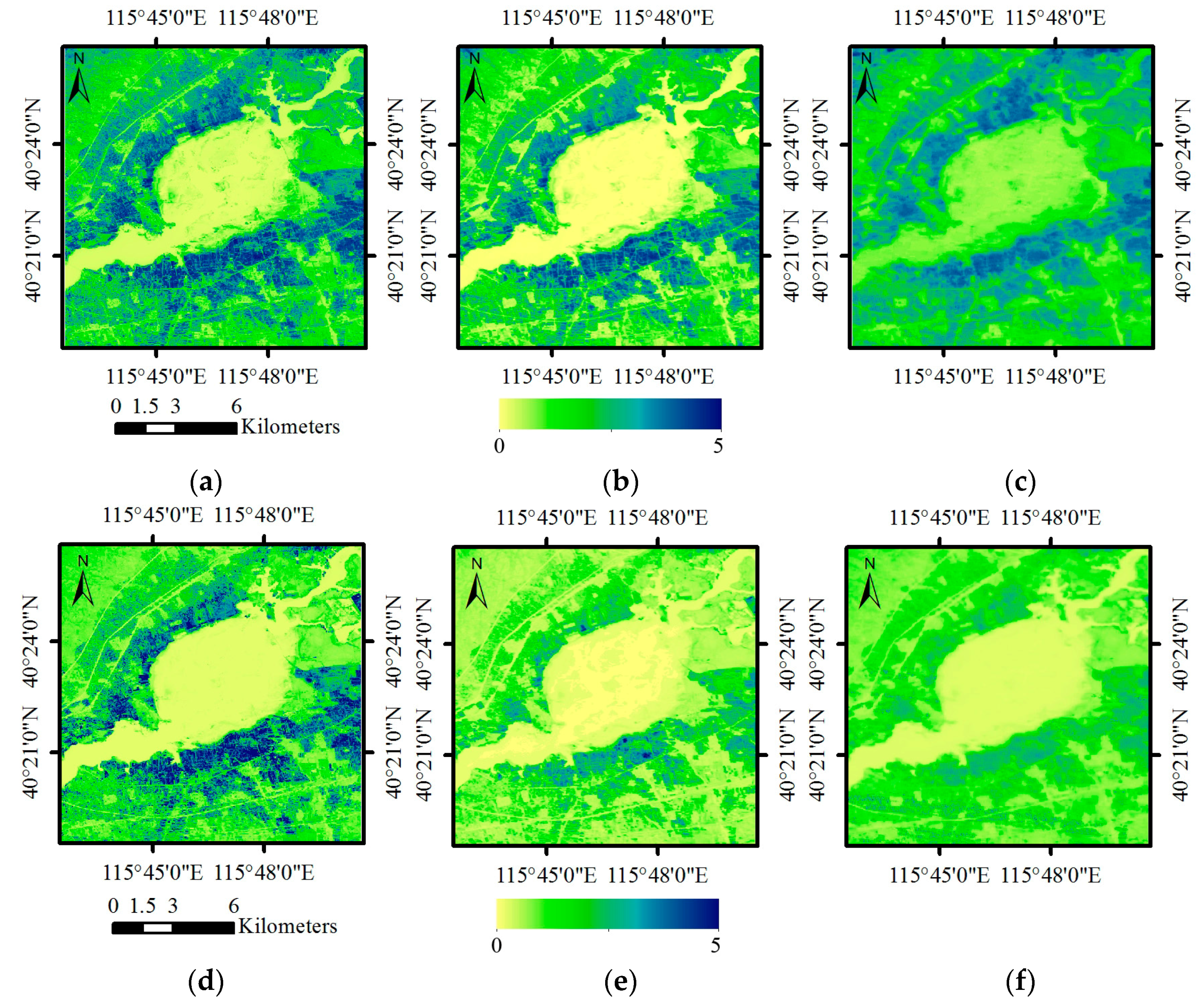
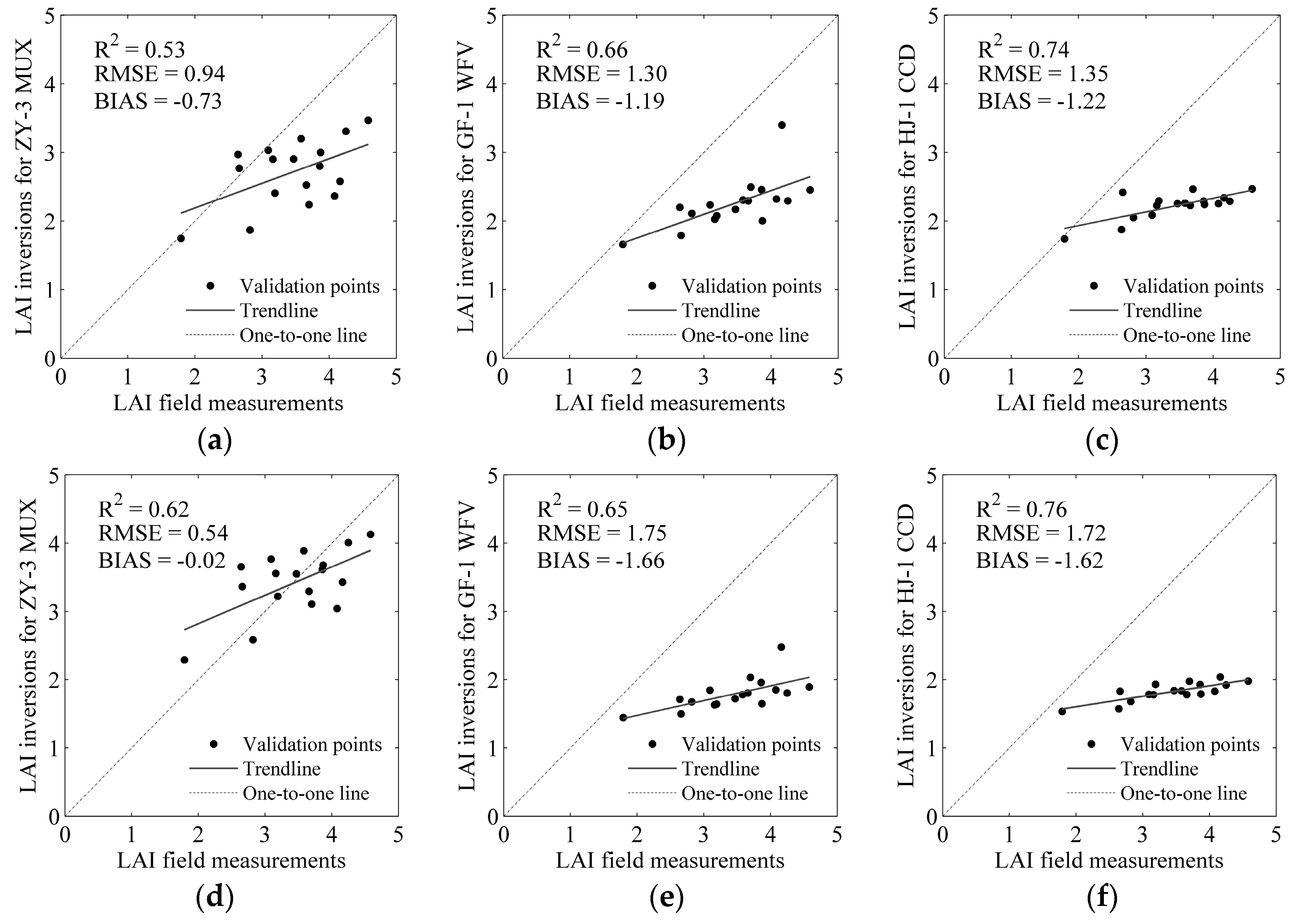
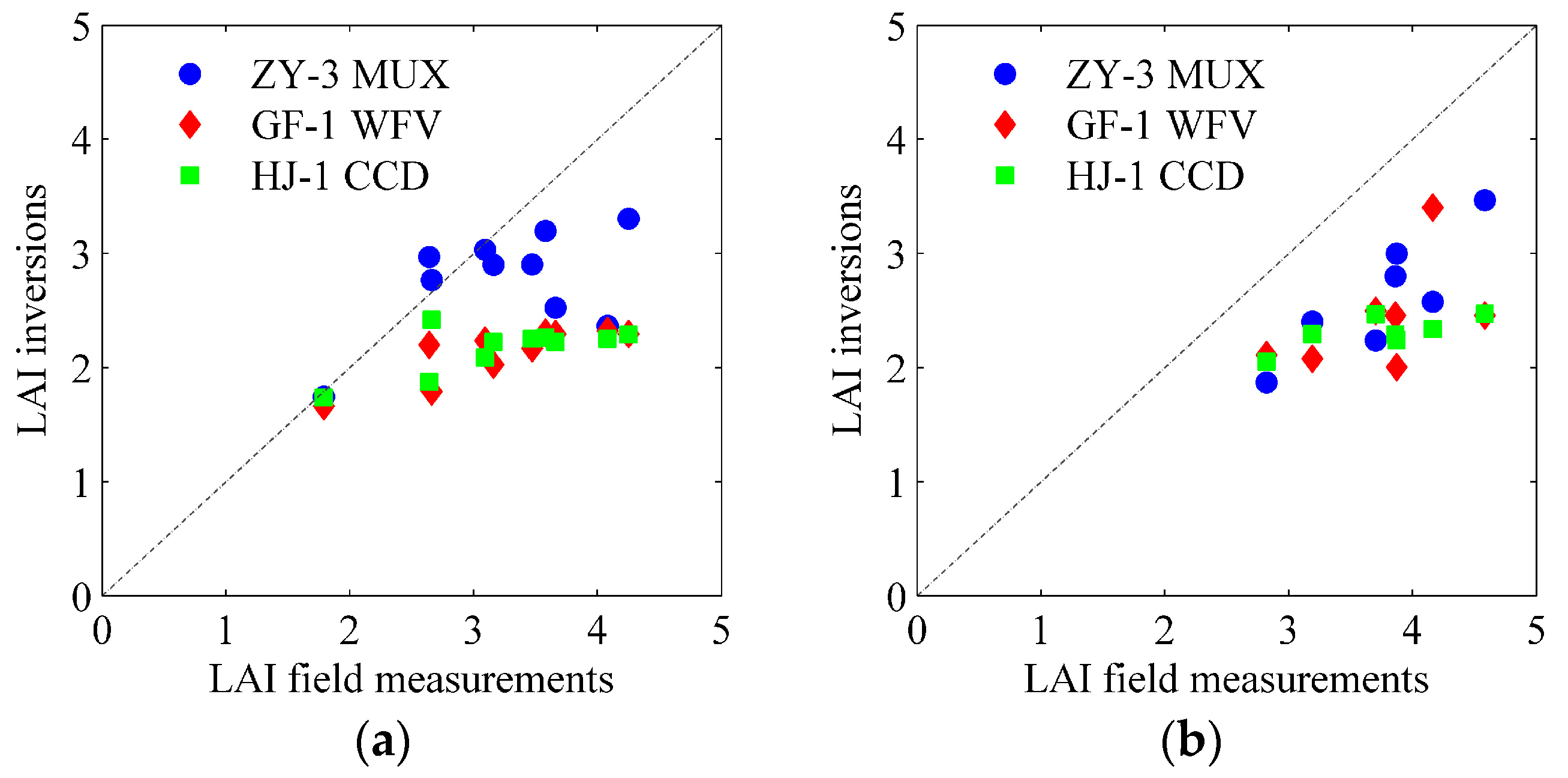
3.1. LAI Validation for ZY-3 MUX, GF-1 WFV and HJ-1 CCD

The LAI inversions for ZY-3 MUX, GF-1 WFV, and HJ-1 CCD based on the proposed LAI method are shown in Figure 4. The LAI inversions from (a) to (c) were inversed from the NDVI-LAI exponential relationships in Table 5, and the LAI inversions from (d) to (f) were inversed from the NIRv-LAI exponential relationships in Table 5. The high LAI values were in the forest and cropland regions around the reservoir, whereas the low LAI values were in the wetland beach and grassland regions in the right corner and bottom of the images. Overall, the spatial variations in these three LAI inversions were similar. However, the values of the LAI inversions for the GF-1 WFV and HJ-1 CCD images were much lower, as is especially apparent in Figure 4c,e,f.
The performances of the proposed LAI estimation method for the ZY-3 MUX, GF-1 WFV, and HJ-1 CCD data were validated based on the LAI field measurements from 17 maize samples (Figure 5). Although the R2 values of the field measurements, compared with the NDVI-LAI inversions from GF-1 WFV (R2 = 0.66) and HJ-1 CCD (R2 = 0.74), were higher than that of ZY-3 MUX (R2 = 0.53), the NDVI-LAI inversions from GF-1 WFV and HJ-1 CCD tended to be systematically underestimated, especially for the higher LAI values. The RMSE and BIAS of the NDVI-LAI inversions from ZY-3 MUX (RMSE = 0.94 and BIAS = −0.73) were lower than those from GF-1 WFV (RMSE = 1.30 and BIAS = −1.19) and HJ-1 CCD (RMSE = 1.35 and BIAS = −1.22). Overall, the performance of the LAI inversed from the NDVI-LAI relationship for ZY-3 MUX was better than that from GF-1 WFV and HJ-1 CCD (Figure 5a–c). In addition, the performance of the method for LAI inversed from the NIRv-LAI relationships for GF-1 WFV and HJ-1 CCD was not sufficient, because the NIRv-LAI relationships largely depended on the reflectance of the NIR band, which was significantly underestimated in the NDVI-LAI inversions (Figure 5e,f). The performance of the method for LAI inversed from the NIRv-LAI relationships was better for ZY-3 MUX (R2 = 0.62, RMSE = 0.54 and BIAS = −0.02) than for GF-1 WFV and HJ-1 CCD (Figure 5d). Because the LAI field measurements were all observed on the same day (31 July 2014), apart from one LAI value of 1.8, the other LAI values varied from 2.5 to 4.5. The concentrated LAI measurements led to small R2 values between the LAI inversions and field measurements, as shown in Figure 5. Moreover, the RMSE and BIAS reflected the systematical underestimation of LAI estimations from GF-1 WFV and HJ-1 CCD.

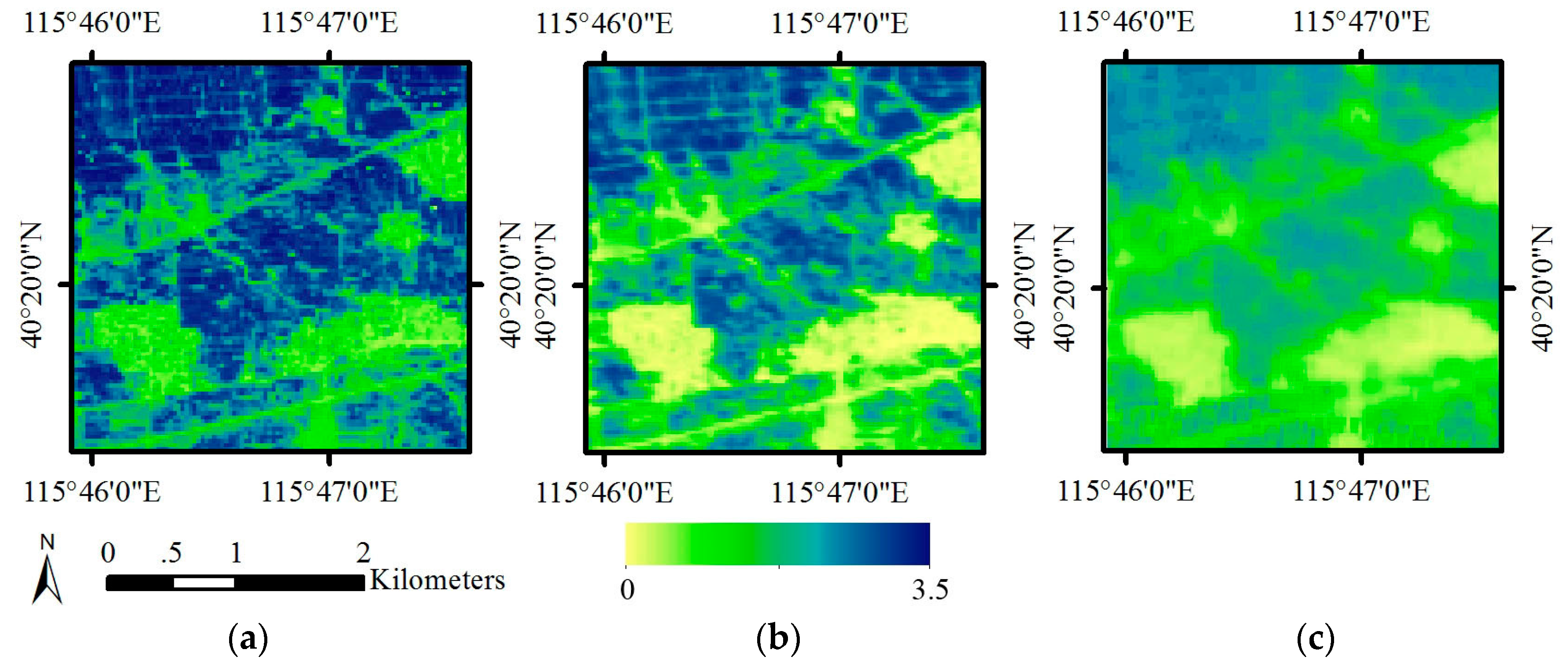
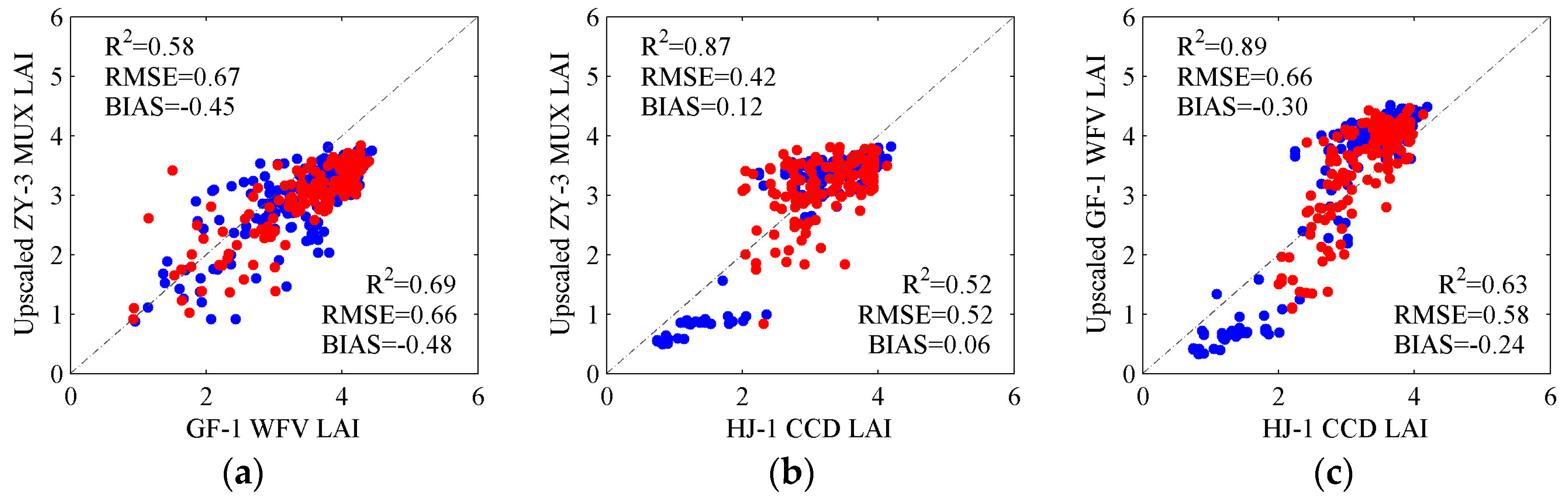
3.2. Influence of Spatial Resolution on LAI Inversion

Spatial resolution influenced the LAI inversions from all the different sensors: the value ranges and accuracies of the LAI inversions both decreased with decreasing spatial resolution (Figure 4 and Figure 5). The spatial representativeness of the LAI field measurements was first assessed by the RAE and CS, according to the methods in Section 3.3 to determine the differences between the LAI inversions from the NDVI-LAI relationships for ZY-3 MUX, GF-1 WFV, and HJ-1 CCD with different spatial resolutions. The LAI inversions from ZY-3 MUX, GF-1 WFV, and HJ-1 CCD were compared with the different spatial representativeness of LAI field measurements, and the results are shown in Figure 6. The performance of the LAI inversions from ZY-3 MUX, GF-1 WFV, and HJ-1 CCD using the LAI field measurements with high spatial representativeness was higher than that obtained using measurements with low spatial representativeness. The LAI inversions using measurements of low spatial resolution exhibited various degrees of underestimation. However, although the performance of the LAI inversions using the LAI field measurements with high spatial representativeness appears to be better in Figure 6a, the LAI inversions for GF-1 WFV and HJ-1 CCD were systematically more underestimated than were those for ZY-3 MUX. It is possible that the size of the pixels of the ZY-3 MUX data was closer to the actual surface. However, the lower spatial resolution of the GF-1 WFV and HJ-1 CCD data recorded more comprehensive information about the surface objects; thus, the vegetation signal was weakened. Therefore, the accuracies of the LAI inversions from the lower-spatial-resolution data were generally lower than those of the higher- spatial-resolution data.
In addition, this study extracted a 3 × 3 km2 range of LAI inversions from the NDVI-LAI relationships to compare the accuracy of LAI inversions among ZY-3 MUX, GF-1 WFV, and HJ-1 CCD at a consistent spatial resolution. The LAI result of ZY-3 MUX was up-scaled to 16 m and 30 m spatial resolution, and the LAI result of GF-1 WFV was up-scaled to 30 m spatial resolution using the upscaling method described in Section 3.3. The up-scaled LAI inversions with 30 m spatial resolution from ZY-3 MUX and GF-1 WFV were compared with the LAI inversion from HJ-1 CCD (Figure 7). The results indicated that the distribution patterns of the LAI inversions were consistent, and that there were higher LAI values in the top left corner of the image near cropland and lower LAI values near roads and in residential areas. However, the LAI inversions that were up-scaled from higher spatial resolution (e.g., ZY-3 MUX and GF-1 WFV) reflected more detail than did the HJ-1 CCD inversion at the same 30 m spatial resolution.
The pixels that were extracted from the LAI inversions in the 3 × 3 km2 area were used to further analyze the differences among the three LAI inversions at the same spatial resolution. The pixels in the subregion were separated into pure pixels with uniform surface types and mixed pixels with different surface types, including different vegetation types, roads, or residential areas. The relationships between the LAI inversions from ZY-3 MUX data that were up-scaled to 16 m spatial resolution and those from GF-1 WFV data and the relationships between the LAI inversions from the ZY-3 MUX or GF-1 WFV data that were up-scaled to 30 m spatial resolution and the LAI inversions from HJ-1 CCD data are shown in Figure 8, for both the pure (blue dots) and mixed (red dots) pixels. Generally, the performances of the LAI inversions between the HJ-1 CCD data and the up-scaled results of the ZY-3 MUX or GF-1 WFV data were preferable for both pure and mixed pixels. The accuracies of the LAI inversions for pure pixels are shown in Figure 8b,c, and these results presented a better agreement between the up-scaled LAI inversions from ZY-3 MUX (R2 = 0.87, RMSE = 0.42 and BIAS = 0.12) or GF-1 WFV (R2 = 0.89, RMSE = 0.66 and BIAS = −0.30) and HJ-1 CCD. In contrast, the up-scaled LAI inversions from ZY-3 MUX and GF-1 WFV, as shown in Figure 8a, did not perform as well for the pure (R2 = 0.58, RMSE = 0.67 and BIAS = −0.45) or the mixed (R2 = 0.69, RMSE = 0.66 and BIAS = −0.48) pixels. The up-scaled LAI inversions for mixed pixels from ZY-3 MUX (R2 = 0.52, RMSE = 0.52 and BIAS = 0.06) and GF-1 WFV (R2 = 0.63, RMSE = 0.58 and BIAS = −0.24) at 30 m spatial resolution were both substantially different from the HJ-1 CCD inversion (Figure 8b,c). In particular, the ZY-3 MUX sensor had much higher performance than the HJ-1 CCD, which demonstrated that the differences between the LAI inversions increased with the increasing spatial resolution between the two sensors.

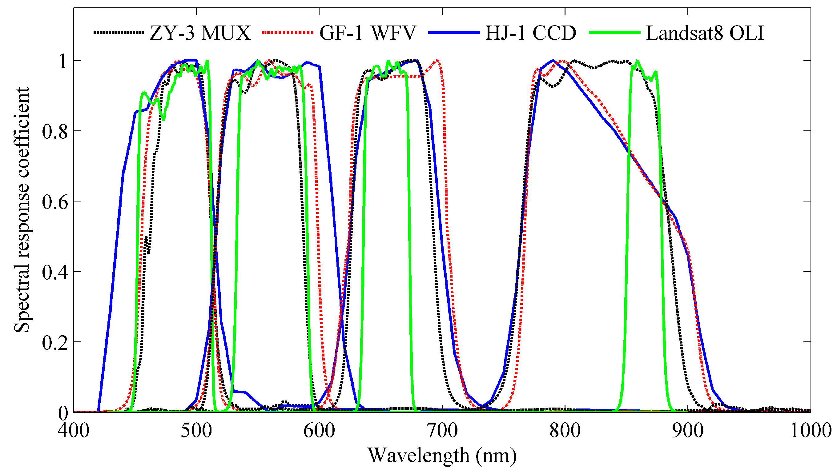
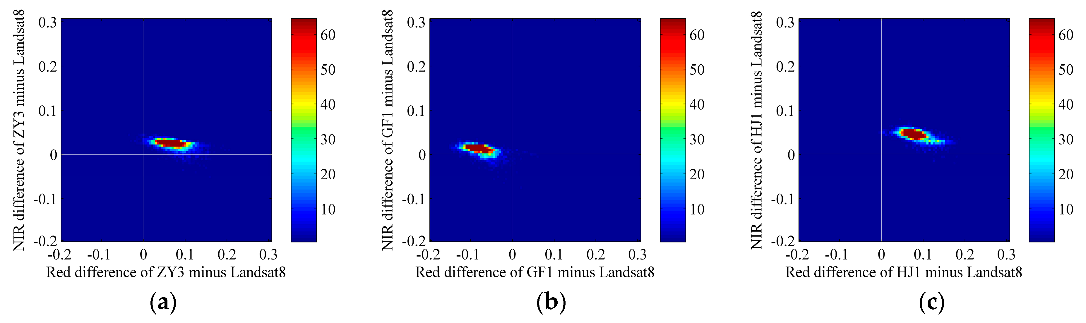
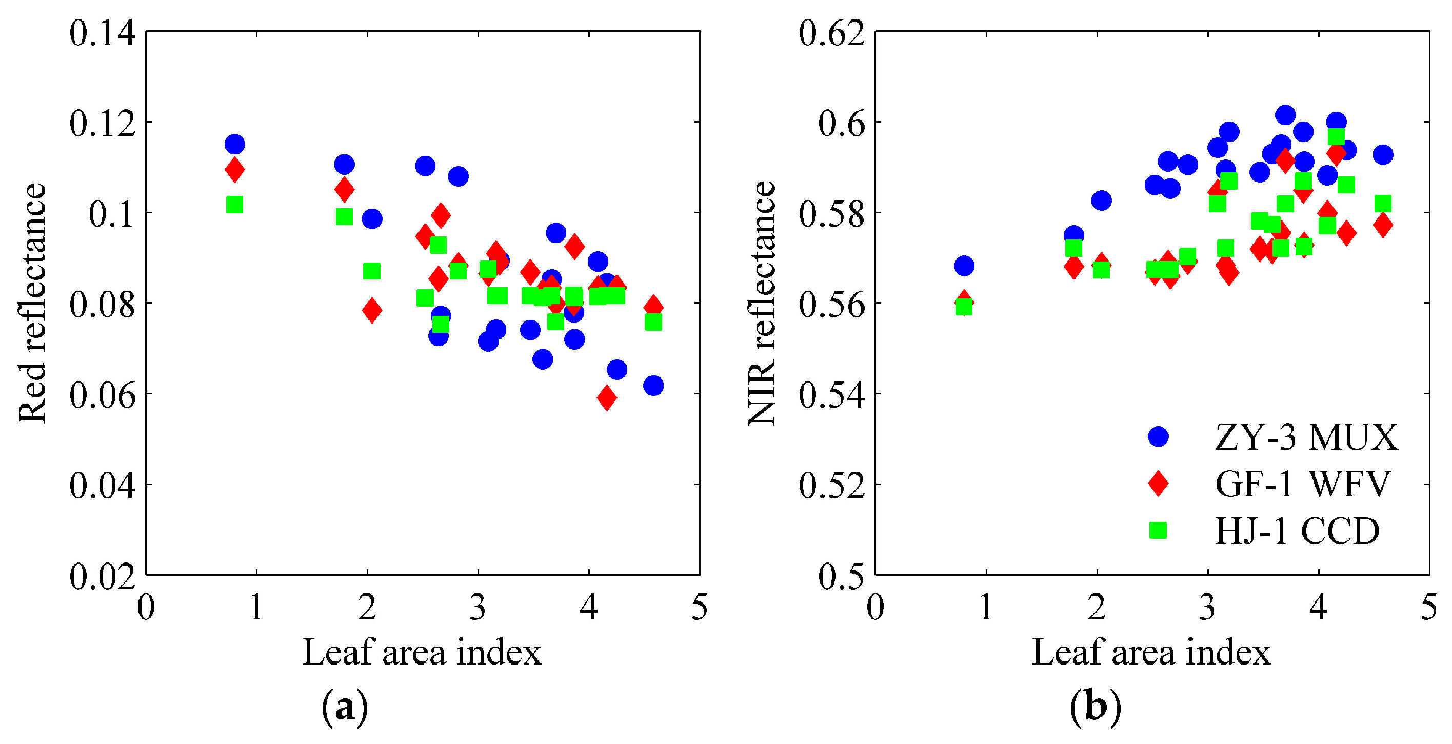
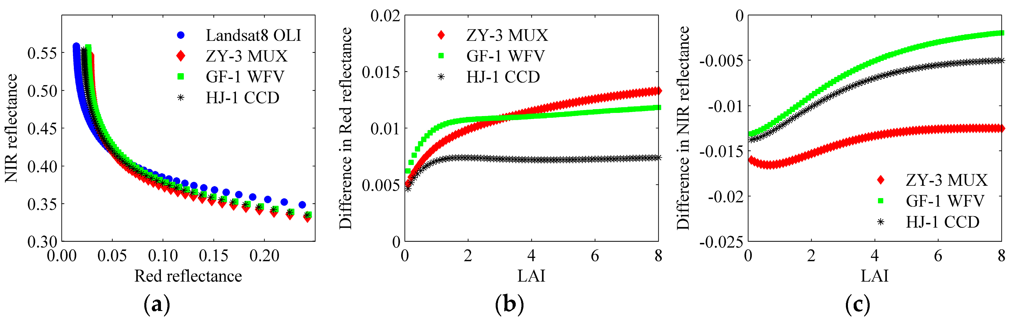
3.3. Comparison of Reflectance among Different Sensors

A correlation analysis was used to compare the accuracy of the reflectance among the three different sensors at different LAI values. The reflectance values of ZY-3 MUX, GF-1 WFV, and HJ-1 CCD in the red and NIR bands were extracted, according to the coordinates of the LAI field measurements. The relationships between the LAI field measurements and the corresponding reflectance in the red and NIR bands are shown in Figure 9. The reflectance values of ZY-3 MUX, GF-1 WFV, and HJ-1 CCD decreased with increasing LAI, and the reflectance values were much more scattered in the red band than in the NIR band (Figure 9a). The R2 values between the reflectance and the LAI were 0.49, 0.50, and 0.59 for ZY-3 MUX, GF-1 WFV, and HJ-1 CCD, respectively. However, the reflectance of the red band for HJ-1 CCD easily reached saturation when the LAI was greater than 3. The reflectance in the NIR band increased with LAI (Figure 9b) in all sensors, and the R2 values between the reflectance and the LAI were higher than in the red band, which were 0.66, 0.45, and 0.56 for ZY-3 MUX, GF-1 WFV, and HJ-1 CCD, respectively. The degree of variation of the NIR reflectance was higher than the variation in the red reflectance. This was especially true for ZY-3 MUX, which had the highest reflectance values. However, the trends of the NIR reflectance variations were more coincident among ZY-3 MUX, GF-1 WFV, and HJ-1 CCD.
To determine the influences of different sensor spectral response functions, the reflectance in the red and NIR bands for Landsat-8 OLI and the three Chinese satellite sensors (i.e., ZY-3 MUX, GF-1 WFV, and HJ-1 CCD) were simulated from the PROSAIL model based on the same values of input variables presented in Table 4, with SZA at 30°, VZA at 0°, and LAI varying from 0 to 8 at intervals of 0.1. The theoretical differences in reflectance in the red or NIR band were compared between the simulations of Landsat-8 OLI and those of ZY-3 MUX, GF-1 WFV, or HJ-1 CCD (Figure 10). The results showed that the individual reflectances of ZY-3 MUX, GF-1 WFV, and HJ-1 CCD were higher than those of Landsat-8 OLI in the red band (Figure 10b) and lower than those of Landsat-8 OLI in the NIR band (Figure 10c). The reflectance in the red band for HJ-1 CCD and that in the NIR band for GF-1 WFV were each close to the corresponding bands of Landsat-8 OLI. The differences in reflectance in the NIR band were larger than those in the red band. These differences occurred because the NIR spectral response function of Landsat-8 OLI was much narrower than those of the Chinese satellite sensors for ZY-3 MUX, GF-1 WFV, and HJ-1 CCD, as shown in Figure 2. In addition, the difference in reflectance between Landsat-8 OLI and each of the Chinese satellite sensors was greatly influenced by the sensor’s spatial resolution. The reflectance that was theoretically closest to that of Landsat-8 OLI was that of HJ-1 CCD with 30 m spatial resolution, followed by that of GF-1 WFV.
To analyze the stability of the different sensors, the actual differences of reflectance in the red and NIR bands were compared between Landsat-8 OLI and each of ZY-3 MUX, GF-1 WFV, and HJ-1 CCD. The reflectance data of the four sensors were compared at the same spatial resolution of 30 m; thus, the mean values of reflectance for ZY-3 MUX and GF-1 WFV were compared with Landsat-8 OLI reflectance values. Approximately 7000 pixels of uniform cropland were extracted from Landsat-8 OLI, ZY-3 MUX, GF-1 WFV, and HJ-1 CCD images. The percentage density plots of reflectance differences between Landsat-8 OLI and each of ZY-3 MUX, GF-1 WFV and HJ-1 CCD in the red and NIR bands are shown in Figure 11. The majority of reflectance values of ZY-3 MUX and HJ-1 CCD were higher than those of Landsat-8 OLI in both the red and NIR bands (Figure 11a,c). Most of the reflectance values of GF-1 WFV were lower than those of Landsat-8 OLI in the red band and higher than those of Landsat-8 OLI in the NIR band (Figure 11b). However, due to the similar observation geometry conditions between ZY-3 MUX and Landsat-8 OLI, with near nadir observations of Landsat-8 OLI and an SZA of 27.67°, the reflectance differences between ZY-3 MUX and Landsat-8 OLI were lower than those between GF-1 WFV or HJ-1 CCD and Landsat-8 OLI (Figure 11a). In addition, the sensor stability in the NIR band was higher than that in the red band for all three Chinese satellite sensors, with lower reflectance differences from Landsat-8 OLI.

4. Discussion

The discrepancies for different instruments or platforms greatly influenced the accuracy of LAI inversion. The factors that influenced LAI inversion included the sensor spectral response function, sun-view geometry, and data preprocessing errors [16,51]. The maximal NDVI difference among ZY-3 MUX, GF-1 WFV, and HJ-1 CCD in theory reached 2.62% due to the different sensor spectral response functions (Figure 10). Because of the similar satellite transit period in the study area, the SZA values of these three sensors were approximately equal, but the VZA difference among these three sensors was approximately 30°. Based on the reflectance in the red and NIR bands in Figure 9, the maximum NDVI difference between ZY-3 MUX, GF-1 WFV, and HJ-1 CCD was 9.74%. The error of geometric correction was less than one pixel for each sensor image in this study. For different sensor resolutions, the one pixel error of geometric correction was 5.8 m for ZY-3 MUX, 16 m for GF-1 WFV and 30 m for HJ-1 CCD. In addition, because of the unstable data quality of HJ-1 CCD, cross-radiometric calibration was performed. In this case, atmospheric correction was achieved based on the method proposed by Zhong et al. [57,59]. After all of the data preprocessing steps, there is still a systematically discrepancies of reflectance (with maximum value of 0.1), both in red and NIR bands when compared with those of Landsat-8 OLI in Figure 11. Therefore, the accuracy of data preprocessing for multiple sensors was the dominant factor that influence the LAI inversion difference among ZY-3 MUX, GF-1 WFV, and HJ-1 CCD.
NIRv, which combined NIR reflectance with the NDVI, was proposed to accurately estimate the global terrestrial gross primary production (GPP) [78]. NIRv is not easily saturated when compared with the NDVI; therefore, it can be applied to improve the LAI estimation. In this study, NIRv was used to estimate LAI from ZY-3 MUX, GF-1 WFV, and HJ-1 CCD. The performance of LAI inversion based on the NIRv-LAI exponential relationship for ZY-3 MUX was best, as shown in Figure 5d. Notably, NIRv depends largely on NIR reflectance. If the NIR reflectance contains noise, the NIRv will deviate more than the NDVI from actual values. NDVI, as a normalized index that can eliminate the fluctuations in the red and NIR bands, and the performance of LAI inversion from the NDVI-LAI relationship was better than that from NIRv-LAI relationship (Figure 5b,c,e,f). In addition, because of the low saturation of NIRv, the superiority of NIRv in LAI inversion will be more apparent when applied for the inversion of high LAI values, such as those of the forests, but not for small values, such as those of the crops as analyzed in this paper.
Currently, the LAI estimation methods at the regional scale are generally based on a single sensor. The primary restriction for generating regional LAI products with moderate to high spatial resolution is the limited number of sensor observations during a specific period. The multi-sensor data during a specific period can greatly increase the number of observations and improve the accuracy of LAI inversion. The sensors with similar spatial resolution, such as ZY-3 MUX, GF-1 WFV, HJ-1 CCD, Landsat-8 OLI, and Sentinel-2, provide a combined multi-sensor dataset for generating LAI products with moderate to high resolutions. The multi-sensor data have more VZA, and the multi-angular observations from multiple sensors are helpful for improving the accuracy of LAI inversion. However, due to the differences in sensor characteristics, geometric and radiometric normalization between different sensors are necessary.

5. Conclusions

This study analyzed the application of LAI inversed from ZY-3 MUX, GF-1 WFV, and HJ-1 CCD data. The method of LAI extraction was based on the SVI-LAI relationship for ZY-3 MUX, GF-1 WFV, and HJ-1 CCD, which was simulated from the PROSAIL model. The LAI inversions were validated using LAI field measurements of maize in Huailai, Hebei Province, China. Regarding the sensor band settings of three Chinese satellite sensors (ZY-3 MUX, GF-1 WFV, and HJ-1 CCD), the performances of these satellite sensors were comparable to that of Landsat-8 OLI. However, the reflectance of the ZY-3 MUX, GF-1 WFV, and HJ-1 CCD images, which was influenced by SZA, VZA, and data processing methods, differed to varying degrees from the reflectance of the Landsat-8 OLI image. The ZY-3 MUX with similar observation geometry conditions as those of Landsat-8 OLI, showed better performance than did GF-1 WFV and HJ-1 CCD in the study area. When compared with the LAI field measurements, the results showed that the performances of the LAI that was inversed from the NIRv-LAI exponential relationships for ZY-3 MUX (R2 = 0.62, RMSE = 0.54 and BIAS = −0.02) were better than the others. However, the performances of the LAI that was inversed from the NIRv-LAI relationships for GF-1 WFV and HJ-1 CCD did not perform as well because of the larger variations in the NIR reflectance. In contrast, the LAI inversions from the NDVI-LAI relationships for ZY-3 MUX, GF-1 WFV, and HJ-1 CCD were much more stable because the NDVI is a normalized index that can eliminate the fluctuations in the reflectance in the red and NIR bands. Overall, LAI inversions tended to be systematically underestimated, especially for the higher LAI values. The scaling effects of the different spatial resolutions could not be ignored, which demonstrated that the LAI inversion differences increased with larger variations in the spatial resolution between the two sensors, especially between ZY-3 MUX and HJ-1 CCD, for mixed pixels. However, more vegetation types and multi-temporal data at different spatial resolutions in LAI inversions need further study.

Acknowledgments

This work was supported by the GF6 Project under Grant 30-Y20A03-9003017/18, the National Natural Science Foundation of China (No. 41401393 and No. 41671374).

Author Contributions

Jing Zhao, Jing Li and Qinhuo Liu conceived, designed and produced the method of LAI estimation from ZY-3 MUX, GF-1 WFV and HJ-1 CCD based on the PROSAIL model; Hongyan Wang, Chen Chen and Shanlong Wu accomplished the multi-sensor data preprocessing; Baodong Xu provided the LAI spatial representativeness evaluation.

Conflicts of Interest

The authors declare no conflict of interest.

References

  1. Chen, J.M.; Black, T.A. Defining leaf area index for non-flat leaves. Plant Cell Environ. 1992, 15, 421–429. [Google Scholar] [CrossRef]
  2. Duveiller, G.; Weiss, M.; Baret, F.; Defourny, P. Retrieving wheat green area index during the growing season from optical time series measurements based on neural network radiative transfer inversion. Remote Sens. Environ. 2011, 115, 887–896. [Google Scholar] [CrossRef]
  3. Kobayashi, H.; Suzuki, R.; Kobayashi, S. Reflectance seasonality and its relation to the canopy leaf area index in an eastern siberian larch forest: Multi-satellite data and radiative transfer analyses. Remote Sens. Environ. 2007, 106, 238–252. [Google Scholar] [CrossRef]
  4. Baret, F.; Weiss, M.; Lacaze, R.; Camacho, F.; Makhmara, H.; Pacholcyzk, P.; Smets, B. Geov1: LAI and FAPAR essential climate variables and fcover global time series capitalizing over existing products. Part1: Principles of development and production. Remote Sens. Environ. 2013, 137, 299–309. [Google Scholar] [CrossRef]
  5. Peng, J.; Dan, L.; Dong, W. Estimate of extended long-term LAI data set derived from AVHRR and MODIS based on the correlations between LAI and key variables of the climate system from 1982 to 2009. Int. J. Remote Sens. 2013, 34, 7761–7778. [Google Scholar] [CrossRef]
  6. Clark, D.B.; Olivas, P.C.; Oberbauer, S.F.; Clark, D.A.; Ryan, M.G. First direct landscape-scale measurement of tropical rain forest leaf area index, a key driver of global primary productivity. Ecol. Lett. 2008, 11, 163–172. [Google Scholar] [CrossRef] [PubMed]
  7. Coyne, P.I.; Aiken, R.M.; Maas, S.J.; Lamm, F.R. Evaluating yieldtracker forecasts for maize in western kansas. Agron. J. 2009, 101, 671–680. [Google Scholar] [CrossRef]
  8. Sharma, L.K.; Bali, S.K.; Dwyer, J.D.; Plant, A.B.; Bhowmik, A. A case study of improving yield prediction and sulfur deficiency detection using optical sensors and relationship of historical potato yield with weather data in maine. Sensors 2017, 17, 1095. [Google Scholar] [CrossRef] [PubMed]
  9. Asner, G.P.; Scurlock, J.M.O.; Hicke, J.A. Global synthesis of leaf area index observations: Implications for ecological and remote sensing studies. Glob. Ecol. Biogeogr. 2003, 12, 191–205. [Google Scholar] [CrossRef]
  10. Li, Z.; Tang, H.; Xin, X.; Zhang, B.; Wang, D. Assessment of the MODIS LAI product using ground measurement data and HJ-1A/1B imagery in the meadow steppe of hulunber, China. Remote Sens. 2014, 6, 6242–6265. [Google Scholar] [CrossRef]
  11. Tian, Y.; Woodcock, C.E.; Wang, Y.; Privette, J.L.; Shabanov, N.V.; Zhou, L.; Zhang, Y.; Buermann, W.; Dong, J.; Veikkanen, B.; et al. Multiscale analysis and validation of the MODIS LAI product : II. Sampling strategy. Remote Sens. Environ. 2002, 83, 431–441. [Google Scholar] [CrossRef]
  12. Yang, F.; Sun, J.; Zhang, B.; Yao, Z.; Wang, Z.; Wang, J.; Yue, X. Assessment of MODIS LAI product accuracy based on the PROSAIL model, TM and field measurements. Trans. Chin. Soc. Agric. Eng. 2010, 26, 192–197. [Google Scholar]
  13. Cohen, W.B.; Maiersperger, T.K.; Gower, S.T.; Turner, D.P. An improved strategy for regression of biophysical variables and Landsat ETM+ data. Remote Sens. Environ. 2003, 84, 561–571. [Google Scholar] [CrossRef]
  14. Chen, J.M.; Cihlar, J. Retrieving leaf area index of boreal conifer forests using landsat tm images. Remote Sens. Environ. 1996, 55, 153–162. [Google Scholar] [CrossRef]
  15. Colombo, R.; Bellingeri, D.; Fasolini, D.; Marino, C.M. Retrieval of leaf area index in different vegetation types using high resolution satellite data. Remote Sens. Environ. 2003, 86, 120–131. [Google Scholar] [CrossRef]
  16. Soudani, K.; François, C.; Maire, G.L.; Dantec, V.L.; Dufrêne, E. Comparative analysis of IKONOS, SPOT, and ETM+ data for leaf area index estimation in temperate coniferous and deciduous forest stands. Remote Sens. Environ. 2006, 102, 161–175. [Google Scholar] [CrossRef] [Green Version]
  17. Turner, D.P.; Cohen, W.B.; Kennedy, R.E.; Fassnacht, K.S.; Briggs, J.M. Relationships between leaf area index and Landsat TM spectral vegetation indices across three temperate zone sites. Remote Sens. Environ. 1999, 70, 52–68. [Google Scholar] [CrossRef]
  18. Heiskanen, J. Estimating aboveground tree biomass and leaf area index in a mountain birch forest using aster satellite data. Int. J. Remote Sens. 2006, 27, 1135–1158. [Google Scholar] [CrossRef]
  19. Korhonen, L.; Hadi; Packalen, P.; Rautiainen, M. Comparison of Sentinel-2 and Landsat 8 in the estimation of boreal forest canopy cover and leaf area index. Remote Sens. Environ. 2017, 195, 259–274. [Google Scholar] [CrossRef]
  20. Fassnacht, K.S.; Gower, S.T.; Mackenzie, M.D.; Nordheim, E.V.; Lillesand, T.M. Estimating the leaf area index of north central wisconsin forests using the landsat thematic mapper. Remote Sens. Environ. 1997, 61, 229–245. [Google Scholar] [CrossRef]
  21. He, L.I.; Chen, Z.X.; Jiang, Z.W.; Wen-Bin, W.U.; Ren, J.Q.; Liu, B.; Hasi, T. Comparative analysis of GF-1, HJ-1, and Landsat-8 data for estimating the leaf area index of winter wheat. J. Integr. Agric. 2017, 16, 266–285. [Google Scholar]
  22. Thomas, V.; Noland, T.; Treitz, P.; Mccaughey, J.H. Leaf area and clumping indices for a boreal mixed-wood forest: Lidar, hyperspectral, and landsat models. Int. J. Remote Sens. 2011, 32, 8271–8297. [Google Scholar] [CrossRef]
  23. Wu, M.; Wu, C.; Huang, W.; Niu, Z.; Wang, C. High-resolution leaf area index estimation from synthetic landsat data generated by a spatial and temporal data fusion model. Comput. Electron. Agric. 2015, 115, 1–11. [Google Scholar] [CrossRef]
  24. Ilangakoon, N.T.; Gorsevski, P.V.; Milas, A.S. Estimating leaf area index by bayesian linear regression using terrestrial Lidar, LAI-2200 plant canopy analyzer, and landsat tm spectral indices. Can. J. Remote Sens. 2015, 41, 315–333. [Google Scholar] [CrossRef]
  25. Pu, R. Mapping leaf area index over a mixed natural forest area in the flooding season using ground-based measurements and landsat tm imagery. Int. J. Remote Sens. 2012, 33, 6600–6622. [Google Scholar] [CrossRef]
  26. Zhang, H.; Chen, J.M.; Huang, B.; Song, H.; Li, Y. Reconstructing seasonal variation of landsat vegetation index related to leaf area index by fusing with modis data. IEEE J. Sel. Top. Appl. Earth Obs. Remote Sens. 2014, 7, 950–960. [Google Scholar] [CrossRef]
  27. Nguy-Robertson, A.L.; Gitelson, A.A. Algorithms for estimating green leaf area index in C3 and C4 crops for MODIS, Landsat TM/ETM+, MERIS, Sentinel MSI/OLCI, and venµs sensors. Remote Sens. Lett. 2015, 6, 360–369. [Google Scholar] [CrossRef]
  28. Tang, S.; Chen, J.M.; Zhu, Q.; Li, X.; Chen, M.; Sun, R.; Zhou, Y.; Deng, F.; Xie, D. Lai inversion algorithm based on directional reflectance kernels. J. Environ. Manag. 2007, 85, 638–648. [Google Scholar] [CrossRef] [PubMed]
  29. Eklundh, L. Estimating leaf area index in coniferous and deciduous forests in sweden using landsat optical sensor data. Proc. SPIE 2003, 4879, 379–390. [Google Scholar]
  30. Qu, Y.; Zhang, Y.; Xue, H. Retrieval of 30-m-resolution leaf area index from china HJ-1 CCD data and MODIS products through a dynamic bayesian network. IEEE J. Sel. Top. Appl. Earth Obs. Remote Sens. 2014, 7, 222–228. [Google Scholar]
  31. Walthall, C.; Dulaney, W.; Anderson, M.; Norman, J.; Fang, H.; Liang, S. A comparison of empirical and neural network approaches for estimating corn and soybean leaf area index from landsat ETM+ imagery. Remote Sens. Environ. 2004, 92, 465–474. [Google Scholar] [CrossRef]
  32. González-Sanpedro, M.C.; Toan, T.L.; Moreno, J.; Kergoat, L.; Rubio, E. Seasonal variations of leaf area index of agricultural fields retrieved from landsat data. Remote Sens. Environ. 2008, 112, 810–824. [Google Scholar] [CrossRef]
  33. Chen, B.; Wu, Z.; Wang, J.; Dong, J.; Guan, L.; Chen, J.; Yang, K.; Xie, G. Spatio-temporal prediction of leaf area index of rubber plantation using HJ-1A/1B CCD images and recurrent neural network. ISPRS Photogramm. Remote Sens. 2015, 102, 148–160. [Google Scholar] [CrossRef]
  34. Chen, W.; Cao, C.X.; He, Q.S.; Guo, H.D.; Zhang, H.; Li, R.Q.; Sheng, Z.; Xu, M.; Gao, M.X.; Zhao, J.; et al. Quantitative estimation of the shrub canopy LAI from atmosphere-corrected HJ-1 CCD data in mu us sandland. Sci. China Earth Sci. 2010, 53, 26–33. [Google Scholar] [CrossRef]
  35. Fernandes, R.; Weiss, M.; Camacho, F.; Berthelot, B.; Baret, F.; Duca, R. Development and assessment of leaf area index algorithms for the sentinel-2 multispectral imager. In Proceedings of the Geoscience and Remote Sensing Symposium, Quebec City, QC, Canada, 13–18 July 2014; pp. 3922–3925. [Google Scholar]
  36. Richter, K.; Hank, T.B.; Vuolo, F.; Mauser, W.; D’Urso, G. Optimal exploitation of the Sentinel-2 spectral capabilities for crop leaf area index mapping. Remote Sens. 2012, 4, 561–582. [Google Scholar] [CrossRef] [Green Version]
  37. Verrelst, J.; Rivera, J.P.; Veroustraete, F.; Muñoz-Marí, J.; Clevers, J.G.P.W.; Camps-Valls, G.; Moreno, J. Experimental Sentinel-2 LAI estimation using parametric, non-parametric and physical retrieval methods—A comparison. ISPRS Photogramm. Remote Sens. 2015, 108, 260–272. [Google Scholar] [CrossRef]
  38. Houborg, R.; Mccabe, M.; Cescatti, A.; Gao, F.; Schull, M.; Gitelson, A. Joint leaf chlorophyll content and leaf area index retrieval from landsat data using a regularized model inversion system (regflec). Remote Sens. Environ. 2015, 159, 203–221. [Google Scholar] [CrossRef]
  39. Verrelst, J.; Camps-Valls, G.; Muñoz-Marí, J.; Rivera, J.P.; Veroustraete, F.; Clevers, J.G.P.W.; Moreno, J. Optical remote sensing and the retrieval of terrestrial vegetation bio-geophysical properties—A review. ISPRS Photogramm. Remote Sens. 2015, 108, 273–290. [Google Scholar] [CrossRef]
  40. Jonckheere, I.; Fleck, S.; Nackaerts, K.; Muys, B.; Coppin, P.; Weiss, M.; Baret, F. Methods for leaf area index determination. Part I: Theories, sensors and hemispherical photography. Agric. For. Meteorol. 2004, 121, 19–35. [Google Scholar] [CrossRef]
  41. Price, E. Lai-2200c plant canopy analyzer. In Proceedings of the American Society for Horticultural Science Conference, Orlando, FL, USA, 28–31 July 2014. [Google Scholar]
  42. Leblanc, S.G.; Chen, J.M.; Kwong, M. Tracing radiation and architecture of canopies. Trac manual version 2.1.3. Gastroenterology 2002, 78, 722–727. [Google Scholar]
  43. Decagon Devices, I. Accupar Par/Lai Ceptometer Model Lp-80; Decagon Devices, Inc.: Pullman, WA, USA, 2015. [Google Scholar]
  44. Campos-Taberner, M.; García-Haro, F.J.; Moreno, Á.; Gilabert, M.A.; Sánchez-Ruiz, S.; Martínez, B.; Camps-Valls, G. Mapping leaf area index with a smartphone and gaussian processes. IEEE Geosci. Remote Sens. Lett. 2015, 12, 2501–2505. [Google Scholar] [CrossRef]
  45. Confalonieri, R.; Foi, M.; Casa, R.; Aquaro, S.; Tona, E.; Peterle, M.; Boldini, A.; Carli, G.D.; Ferrari, A.; Finotto, G. Development of an app for estimating leaf area index using a smartphone. Trueness and precision determination and comparison with other indirect methods. Comput. Electron. Agric. 2013, 96, 67–74. [Google Scholar] [CrossRef]
  46. Francone, C.; Pagani, V.; Foi, M.; Cappelli, G.; Confalonieri, R. Comparison of leaf area index estimates by ceptometer and pocketlai smart app in canopies with different structures. Field Crop. Res. 2014, 155, 38–41. [Google Scholar] [CrossRef]
  47. Zhao, J.; Li, J.; Liu, Q.; Fan, W.; Zhong, B.; Wu, S.; Yang, L.; Zeng, Y.; Xu, B.; Yin, G. Leaf area index retrieval combining HJ1/CCD and Landsat 8/OLI data in the heihe river basin, China. Remote Sens. 2015, 7, 6862–6885. [Google Scholar] [CrossRef]
  48. Zhan, Y.; Menga, Q.; Wanga, C.; Li, J.; Zhouab, K.; Li, D. Fractional vegetation cover estimation over large regions using GF-1 satellite data. In Proceedings of the SPIE Asia-Pacific Remote Sensing, Beijing, China, 27–31 October 2014. [Google Scholar]
  49. Jia, K.; Liang, S.; Gu, X.; Baret, F.; Wei, X.; Wang, X.; Yao, Y.; Yang, L.; Li, Y. Fractional vegetation cover estimation algorithm for chinese GF-1 wide field view data. Remote Sens. Environ. 2016, 177, 184–191. [Google Scholar] [CrossRef]
  50. Wang, L.; Niu, Z.; Wang, C.; Huang, W.; Chen, H.; Gao, S.; Li, D.; Muhammad, S. Combined use of airborne lidar and satellite GF-1 data to estimate leaf area index, height, and aboveground biomass of maize during peak growing season. IEEE J. Sel. Top. Appl. Earth Obs. Remote Sens. 2015, 8, 4489–4501. [Google Scholar]
  51. Wang, L.; Yang, R.; Tian, Q.; Yang, Y.; Zhou, Y.; Sun, Y.; Mi, X. Comparative analysis of GF-1 WFV, ZY-3 MUX, and HJ-1 CCD sensor data for grassland monitoring applications. Remote Sens. 2015, 7, 2089–2108. [Google Scholar] [CrossRef]
  52. Zeng, Y.; Li, J.; Liu, Q.; Li, L.; Xu, B.; Yin, G.; Peng, J. A sampling strategy for remotely sensed lai product validation over heterogeneous land surfaces. IEEE J. Sel. Top. Appl. Earth Obs. Remote Sens. 2014, 7, 3128–3142. [Google Scholar] [CrossRef]
  53. Satellite Surveying and Mapping Application Center (SASMAC) of National Administration of Surveying Mapping and Geo-Information of China (NASG). Available online: http://sjfw.sasmac.cn/en.html (accessed on 14 December 2017).
  54. Gaofen Satellite Data and Information Service System (GFDIS). Available online: http://210.72.27.32:8080/SNFFWeb/WebUI/Main/HomePage.jsp (accessed on 14 December 2017).
  55. China Centre for Resources Satellite Data and Application (CRESDA). Available online: http://www.cresda.com/CN/index.shtml (accessed on 14 December 2017).
  56. United States Geological Survey (USGS) Earthexplorer. Available online: https://earthexplorer.usgs.gov/ (accessed on 14 December 2017).
  57. Zhong, B.; Zhang, Y.; Du, T.; Yang, A.; Lv, W.; Liu, Q. Cross-calibration of hj-1/ccd over a desert site using landsat etm imagery and aster gdem product. IEEE Trans. Geosci. Remote Sens. 2014, 1–17. [Google Scholar]
  58. Zhang, Y.H. HJ1-CCD Cross Radiometric Calibration. Master’s Thesis, Shandong University of Science and Technology, Shandong, China, 2011. [Google Scholar]
  59. Zhong, B. Improved estimation of aerosol optical depth from Landsat TM/ETM+ imagery over land. In Proceedings of the IEEE International Geoscience and Remote Sensing Symposium (IGARSS), Vancouver, BC, Canada, 24–29 July 2011; pp. 3304–3307. [Google Scholar]
  60. Kuusk, A. The hot spot effect in plant canopy reflectance. In Photon-Vegetation Interactions: Applications in Optical Remote Sensing and Plant Ecology; Myneni, R., Ross, J., Eds.; Springer: New York, NY, USA, 1991; pp. 139–159. [Google Scholar]
  61. Verhoef, W. Light scattering by leaf layers with application to canopy reflectance modeling: The sail model. Remote Sens. Environ. 1984, 16, 125–141. [Google Scholar] [CrossRef]
  62. Jacquemoud, S.; Baret, F. Prospect: A model of leaf optical properties spectra. Remote Sens. Environ. 1990, 34, 75–91. [Google Scholar] [CrossRef]
  63. Jacquemoud, S.; Verhoef, W.; Baret, F.; Bacour, C.; Zarco-Tejada, P.J.; Asner, G.P.; François, C.; Ustin, S.L. PROSPECT + SAIL models: A review of use for vegetation characterization. Remote Sens. Environ. 2009, 113, S56–S66. [Google Scholar] [CrossRef]
  64. Jacquemoud, S.; Verhoef, W.; Baret, F.; Zarco-Tejada, P.J.; Asner, G.P.; Francois, C.; Ustin, S.L. PROSPECT+SAIL: 15 years of use for land surface characterization. In Proceedings of the IEEE International Conference on Geoscience and Remote Sensing Symposium (IGARSS), Denver, CO, USA, 31 July–4 August 2006; pp. 1992–1995. [Google Scholar]
  65. Xiao, Y.; Zhao, W.; Zhou, D.; Gong, H. Sensitivity analysis of vegetation reflectance to biochemical and biophysical variables at leaf, canopy, and regional scales. IEEE Trans. Geosci. Remote Sens. 2014, 52, 4014–4024. [Google Scholar] [CrossRef]
  66. Zeng, X.; Dickinson, R.E.; Walker, A.; Shaikh, M.; Defries, R.S.; Qi, J. Derivation and evaluation of global 1-km fractional vegetation cover data for land modeling. J. Appl. Meteorol. 2000, 39, 826–839. [Google Scholar] [CrossRef]
  67. Li, X.; Zhang, J. Derivation of the green vegetation fraction of the whole china from 2000 to 2010 from modis data. Earth Interact. 2016, 20, 1–8. [Google Scholar] [CrossRef]
  68. Sharma, L.K.; Bu, H.; Franzen, D. Active Optical Sensor Algorithm for Corn Yield Prediction and Corn Side Dress Nitrogen Rate Aid; North Dakota State University: Fargo, ND, USA, 2014. [Google Scholar]
  69. Sharma, L.K.; Bu, H.; Denton, A.; Franzen, D.W. Active-optical sensors using red ndvi compared to red edge ndvi for prediction of corn grain yield in North Dakota, U.S.A. Sensors 2015, 15, 27832–27853. [Google Scholar] [CrossRef] [PubMed]
  70. Bu, H.; Sharma, L.K.; Denton, A.; Franzen, D.W. Comparison of satellite imagery and ground-based active optical sensors as yield predictors in sugar beet, spring wheat, corn, and sunflower. Agron. J. 2017, 109, 1–10. [Google Scholar] [CrossRef]
  71. Sharma, L.K.; Bu, H.; Franzen, D.W. Comparison of two ground-based active-optical sensors for in-season estimation of corn (Zea mays, L.) yield. J. Plant Nutr. 2016, 39, 957–966. [Google Scholar] [CrossRef]
  72. Sharma, L.K. Evaluation of Active Optical Ground-Based Sensors to Detect Early Nitrogen Deficiencies in Corn. Ph.D. Thesis, North Dakota State University of Agriculture and Applied Sciences, Fargo, ND, USA, April 2014. [Google Scholar]
  73. Franzen, D.W.; Sharma, L.K.; Bu, H.; Denton, A. Evidence for the ability of active-optical sensors to detect sulfur deficiency in corn. Agron. J. 2016, 108, 1–5. [Google Scholar] [CrossRef]
  74. Bu, H.; Sharma, L.K.; Denton, A.; Franzen, D.W. Sugar beet yield and quality prediction at multiple harvest dates using active-optical sensors. Agron. J. 2016, 108, 273–284. [Google Scholar] [CrossRef]
  75. Sharma, L.K.; Bu, H.; Franzen, D.W.; Denton, A. Use of corn height measured with an acoustic sensor improves yield estimation with ground based active optical sensors. Comput. Electron. Agric. 2016, 124, 254–262. [Google Scholar] [CrossRef]
  76. Sharma, L.K.; Franzen, D.W. Use of corn height to improve the relationship between active optical sensor readings and yield estimates. Precis. Agric. 2012, 15, 331–345. [Google Scholar] [CrossRef]
  77. Tian, Q.; Luo, Z.; Chen, J.M.; Chen, M.; Hui, F. Retrieving leaf area index for coniferous forest in xingguo county, China with Landsat ETM+ images. J. Environ. Manag. 2007, 85, 624–627. [Google Scholar] [CrossRef] [PubMed]
  78. Badgley, G.; Field, C.B.; Berry, J.A. Canopy near-infrared reflectance and terrestrial photosynthesis. Sci. Adv. 2017, 3, 1–5. [Google Scholar] [CrossRef] [PubMed]
  79. Xu, B.; Li, J.; Liu, Q.; Huete, A.R.; Yu, Q.; Zeng, Y.; Yin, G.; Zhao, J.; Yang, L. Evaluating spatial representativeness of station observations for remotely sensed leaf area index products. IEEE J. Sel. Top. Appl. Earth Obs. Remote Sens. 2016, 9, 3267–3282. [Google Scholar] [CrossRef]
  80. Zhu, X.; Feng, X.; Zhao, Y. Scale effect and error analysis of crop LAI inversion. J. Remote Sens. 2010, 14, 579–592. [Google Scholar]
Figure 1. The geographic location of the study area of ZY-3 MUX based on the false color composite (NIR-red-green) (a), and the subset study area with leaf area index (LAI) field measurements for maize (yellow dots) (b).
Remotesensing 10 00068 g001
Figure 2. Spectral response curves for ZY-3 MUX, GF-1 WFV, and HJ-1 CCD from CRESDA, and for Landsat-8 OLI from USGS.
Remotesensing 10 00068 g002
Figure 3. Flowchart of the LAI inversion method based on ZY-3 MUX, GF-1 WFV, and HJ-1 CCD.
Remotesensing 10 00068 g003
Figure 4. LAI inversion results for ZY-3 MUX (a,d), GF-1 WFV (b,e), and HJ-1 CCD (c,f) in Huailai, Hebei Province.
Remotesensing 10 00068 g004
Figure 5. Comparisons of the LAI inversions with the field measurements for ZY-3 MUX (a,d), GF-1 WFV(b,e), and HJ-1 CCD (c,f).
Remotesensing 10 00068 g005
Figure 6. Validation of the LAI inversions from ZY-3 MUX, GF-1 WFV, and HJ-1 CCD using field data with high spatial representativeness (a) and low spatial representativeness (b).
Remotesensing 10 00068 g006
Figure 7. LAI inversions up-scaled to 30 m spatial resolution from ZY-3 MUX (a), GF-1 WFV (b), and HJ-1 CCD (c).
Remotesensing 10 00068 g007
Figure 8. LAI inversions up-scaled to 16 m spatial resolution from ZY-3 MUX plotted against GF-1 WFV LAI inversions (a) and LAI inversions up-scaled to 30 m spatial resolution from ZY-3 MUX (b) or GF-1 WFV (c) plotted against HJ-1 CCD LAI inversions for pure (blue dots) and mixed (red dots) pixels.
Remotesensing 10 00068 g008
Figure 9. Reflectance in the red band (a) and the NIR band (b) varied with LAI field measurements for ZY-3 MUX, GF-1 WFV, and HJ-1 CCD.
Remotesensing 10 00068 g009
Figure 10. Reflectance in the red and NIR bands with LAI from 0 to 8 at 0.1 intervals for ZY-3 MUX, GF-1 WFV, HJ-1 CCD, and Landsat-8 OLI (a), and difference in reflectance in the red (b) and NIR (c) bands between Landsat-8 OLI and each of ZY-3 MUX, GF-1 WFV, and HJ-1 CCD for maize simulations.
Remotesensing 10 00068 g010
Figure 11. Density scatter plots of the reflectance difference in the red and NIR bands between Landsat-8 OLI and each of ZY-3 MUX (a), GF-1 WFV (b), and HJ-1 CCD (c) for croplands.
Remotesensing 10 00068 g011
Table 1. Technical specification of the ZY-3 MUX, GF-1 WFV, and HJ-1 CCD cameras.
SensorZY-3 MUXGF-1 WFVHJ-1 CCD
Spectral characteristicsBandsWavelength (μm)BandsWavelength (μm)BandsWavelength (μm)
10.45–0.5210.45–0.5210.43–0.52
20.52–0.5920.52–0.5920.52–0.60
30.63–0.6930.63–0.6930.63–0.69
40.77–0.8940.77–0.8940.76–0.90
Spatial resolution (m)5.81630
Radiometric resolution (Bit)10108
Swath width (km)51200 (single); 800 (4 cameras)360 (single); 700 (two)
Revisit time (days)544
Table 2. Satellite data acquisition information for ZY-3 MUX, GF-1 WFV, HJ-1 CCD and Landsat-8 OLI.
SensorDateLocal TimeSolar Zenith AngleSolar Azimuth AngleView Zenith Angle (Mean)View Azimuth Angle (Mean)
ZY-3 MUX2014072711:15:2325.28°216.38°216.38°
GF-1 WFV2014072711:50:1922.08°201.62°29.97°74.57°
HJ-1 CCD2014072810:00:0934.97°295.49°25°53.59°
Landsat-8 OLI2014072510:59:3427.67°131.88°95.31°
Table 3. The calibration coefficients and extraterrestrial solar irradiance values for ZY-3 MUX, GF-1 WFV, and HJ-1 CCD.
SensorHJ-1 CCDGF-1 WFVZY-3 MUX
GainOffset E S U N λ GainOffset E S U N λ GainOffset E S U N λ
Band 11.14514.63441929.810.17130.00001968.120.25090.00001958.30
Band 21.16604.09821831.140.16000.00001841.690.23380.00001855.71
Band 30.76473.73601549.820.14970.00001540.300.18850.00001548.72
Band 40.75580.73851078.320.14350.00001069.530.20350.00001085.60
Table 4. The input variables for the PROSAIL model used to generate the forward simulation.
ParametersAbbreviationsUnitsValue RangeInterval
Leaf mesophyll structureN-1.518-
Leaf chlorophyll-a and -b contentCabμg/cm40–6010
Leaf dry matter contentCmg/cm0.003662-
Leaf water contentCwcm0.0131-
Carotenoid contentCarμg/cm10-
Brown pigment contentCbrown-0.05-
Average leaf inclination angleALA°40–7010
Hot-spotHot-spot-0.1-
Leaf area indexLAIm2/m20–80.1
Solar zenith angleSZA°0–851
View zenith angleVZA°0–351
Table 5. The SVI-LAI exponential relationships for ZY-3 MUX, GF-1 WFV, and HJ-1 CCD.
SVIsNDVI-LAI RelationshipNIRv-LAI Relationship
ExpressionR2ExpressionR2
ZY-3 MUXLAI = 0.0484 exp(5.2397 * NDVI)0.91LAI = 0.1725 exp(6.4087 * NIRv)0.98
GF-1 WFVLAI = 0.0385 exp(5.4728 * NDVI)0.92LAI = 0.1578 exp(5.6711 * NIRv)0.98
HJ-1 CCDLAI = 0.0380 exp(5.4241 * NDVI)0.91LAI = 0.1543 exp(5.6960 * NIRv)0.98

