The Role of Resolution in the Estimation of Fractal Dimension Maps From SAR Data


1
Department of Electrical Engineering and Information Technology, University of Naples Federico II, Via Claudio 21, 80125 Napoli, Italy
2
Institute for Electromagnetic Sensing of the Environment, Research National Council (CNR), Via Diocleziano 328, 80124 Napoli, Italy
*
Author to whom correspondence should be addressed.
Remote Sens. 2018, 10(1), 9; https://doi.org/10.3390/rs10010009
Submission received: 29 September 2017
/
Revised: 13 November 2017
/
Accepted: 20 December 2017
/
Published: 22 December 2017
(This article belongs to the Special Issue Advances in SAR: Sensors, Methodologies, and Applications)
Abstract
:This work is aimed at investigating the role of resolution in fractal dimension map estimation, analyzing the role of the different surface spatial scales involved in the considered estimation process. The study is performed using a data set of actual Cosmo/SkyMed Synthetic Aperture Radar (SAR) images relevant to two different areas, the region of Bidi in Burkina Faso and the city of Naples in Italy, acquired in stripmap and enhanced spotlight modes. The behavior of fractal dimension maps in the presence of areas with distinctive characteristics from the viewpoint of land-cover and surface features is discussed. Significant differences among the estimated maps are obtained in the presence of fine textural details, which significantly affect the fractal dimension estimation for the higher resolution spotlight images. The obtained results show that if we are interested in obtaining a reliable estimate of the fractal dimension of the observed natural scene, stripmap images should be chosen in view of both economic and computational considerations. In turn, the combination of fractal dimension maps obtained from stripmap and spotlight images can be used to identify areas on the scene presenting non-fractal behavior (e.g., urban areas). Along this guideline, a simple example of stripmap-spotlight data fusion is also presented.

1. Introduction
Cosmo/SkyMed synthetic aperture radar (SAR) multi-operational capabilities allow the observation of a scene at different spatial scales, i.e., with different levels of detail. Usually, the choice of the operational mode better fitting a specific application is dictated by a trade-off between resolution and coverage. In particular, in the case of Cosmo/SkyMed the range of attainable resolutions spans from about 1 m in enhanced spotlight mode, with a coverage of 10 km, to about 100 m in scansar huge region mode, with a coverage of about 200 km, whereas the stripmap mode achieves a resolution of 3 m, with a coverage of 40 km. In this context, stripmap images, or even better, scansar images, are well suited for large-scale applications, whereas spotlight products can be fruitfully used for local-scale analyses, able to provide more detailed information on the observed scene. The combined use of multi-operational data, therefore, can be set in the framework of a multi-scale approach, in which coarse resolution images can provide the necessary regional-scale survey of the area of interest, while high resolution images can be used to refine the analysis on a local scale. Regarding the analysis of natural surfaces, the mentioned multi-scale approach can be used to gain the required information investigating different spatial scales. In fact, the physical and geometrical information regarding the scene under survey can present strong variations, which cannot be fully appreciated through low-resolution SAR data, which, in turn, allow only the estimation of somehow averaged quantities.
When the focus is on surface roughness, fractal models represent the best way to model the behavior of natural surfaces [1,2,3,4,5,6,7,8,9,10,11,12]. The fractal dimension is a concise and meaningful entity, bearing meaningful physical information regarding the geometrical and geophysical characterization of a natural surface [5,6,7,8,9]. In particular, geologists usually use the fractal dimension to model the roughness of natural surfaces, because it is not dependent on the size of the observed surface. In fact, a typical problem of classical statistical roughness descriptors, such as the height standard deviation and correlation length, lies in their dependence on the observation scale and on the extension of the surface from which they are estimated [5,6,7,8,9].
The use of fractal concepts in the remote-sensing community is a long-standing topic, testified by applications regarding image analysis [13], and, in particular, SAR image segmentation [14,15] and feature detection [16,17]. However, all the mentioned works are based on the estimation of fractal parameters of image texture, leaving aside the problem of investigating how the fractal dimension of the observed surfaces is related to the amplitude values of image pixels. This kind of analysis was first considered in Pentland [18], and Kube and Pentland [19] for the case of optical images of Lambertian natural surfaces; this pioneering work was extended to non-Lambertian fractal surfaces in Korvin [20]. More recently this analysis has been performed for the case of SAR imaging: in particular, in Di Martino et al. [21,22] the authors introduced appropriate models and algorithms, allowing for the estimation of the fractal dimension of an observed surface from a SAR amplitude image. Therefore, while works [14,15,16,17] were based on the introduction of convenient fractal-based parameters to perform image processing tasks, without entering the problem of associating to them a clear physical meaning, the estimation framework of Di Martino et al. [21,22] provides estimates of the fractal dimension of the observed surface, i.e., a parameter with a clear physical meaning that can be easily managed by physicists and geologists for the characterization of natural phenomena. Moreover, works [21,22] forerun (and partly stimulated) the development of SAR processing techniques based on the use of fractal dimension: indeed, recently fractal dimension has been fruitfully used in SAR interferometry, to support coregistration [23], regularization [24], and phase unwrapping [25], and in SAR speckle filtering [26,27]. All these techniques benefit from the availability of accurate estimates of the surface fractal dimension.
In more detail, in Di Martino et al. [21,22] the estimation of the surface fractal dimension from a SAR amplitude image is performed exploiting a sliding window scouring the whole image, thus allowing the generation, as output, of a new value-added SAR product, the fractal dimension map, i.e., a point-by-point map of the estimated fractal dimension of the imaged surface, accounting for local variations of the surface fractal dimension. Some properties of the technique we propose are remarkable [28]. The fractal dimension clearly depends on a single feature of the observed scene, namely its roughness. From this viewpoint, the fractal dimension is one of the few parameters retrievable from SAR data that allows the separation of the influence of a single physical parameter (in particular, the roughness) from the others involved in SAR image formation. Actually, in many practical situations, the post-processing of SAR images provides products showing a significant dependence on the acquisition geometry of the employed SAR image, and this is the major disadvantage from the end-user viewpoint. For instance, the severe dependence on the SAR acquisition geometry leads to classification maps that are not easily comparable and cannot be straightforwardly managed by non-expert SAR users, whenever they are obtained from SAR images acquired from different satellite tracks. Conversely, the estimation of the fractal dimension maps is almost independent of the acquisition geometry. In fact, in Di Martino et al. [28] we analyzed a wide set of multi-angle SAR images of the same area and verified that the estimated fractal dimension maps are dependent neither on the sensor look angle nor on the local incidence angle, at least in the hypothesis of validity of the theoretical model (i.e., on natural surfaces). Furthermore, in Di Martino et al. [29] we demonstrated that the maps are not dependent on polarization, at least when co-polarized channels are considered.
Due to the above-mentioned properties, the fractal dimension maps are value-added SAR products that can have a significant impact on the end users’ community. For this reason, in the present paper we investigate the role of resolution, in order to unveil possible dependencies on the surface spatial scales involved in the estimation. For purely fractal surfaces, the fractal dimension keeps constant over all the spatial scales; however, it must be noted that, since the fractional Brownian motion (fBm) surface root mean square (rms) slope decreases as the observation scale increases, at larger observation scales the small-slope hypothesis is more easily satisfied: from this viewpoint, stripmap images are more convenient than spotlight images. In conclusion, we expect that in natural, homogeneous (at the scale of window size) areas the estimated fractal dimension is the same on spotlight and stripmap images, except in the uncommon cases in which the small-slope assumption is satisfied for the stripmap image and not satisfied for the spotlight image. It must be also noted that, sometimes, actual natural surfaces present multifractal behavior, i.e., their fractal dimension changes according to the spatial scale [5,8,9]. This may be another source of difference between the fractal dimension maps obtained from spotlight and stripmap images. Finally, in areas containing man-made objects the employed fractal model does not hold, and since such objects are usually strongly scale-dependent, we expect that the estimated fractal dimension obtained from stripmap and spotlight images can be different.
For the analysis, we use two sets of COSMO-SkyMed stripmap and enhanced spotlight SAR images relevant to the areas of Bidi in Burkina Faso and Naples in Italy. All the images were acquired with similar look angles, between 31° and 33°. Two subsets were cropped from each image as representative of different kind of land-cover and texture properties: they span from a homogeneous bare-soil scenario to a very heterogeneous urban scenario. In this way, we are able to investigate the behavior of the algorithm according to different regimes of validity of the theoretical model. In fact, the theoretical model was originally developed for bare-soil natural surfaces, which can be conveniently modeled through fractals. For such natural surfaces, we expect that the estimated fractal dimension maps do not significantly depend on the employed resolution, due to the scale-invariance property of fractal objects. Accordingly, the same results should be obtained from stripmap and spotlight images. This is the first property that we want to verify in this paper. However, in the presence of man-made objects, or other non-fractal objects, even if the theoretical model does not hold and the algorithm does not provide a true fractal dimension, the estimated meta-parameter can provide meaningful information, which can be used for the characterization of the area of interest [30]. In this case we cannot a priori expect that the estimated fractal dimension does not depend on resolution, and it is of interest to verify the behavior of the obtained results at different resolutions. The analysis is performed within a statistical framework, along the same guidelines of Di Martino et al. [28]. However, we also present results regarding the joint use (on a pixel basis) of the fractal dimension maps obtained from the stripmap and the spotlight images, where we try to identify fine textural details related to specific land-cover classes.
The paper is organized as follows. In Section 2 the theoretical and methodological background is summarized and the remarkable properties presented by the fractal dimension maps are detailed. In Section 3 we present the experimental setup and the statistical analysis of the obtained maps, along with an example of stripmap–spotlight data fusion. Finally, conclusions and relevant suggestions are reported in Section 4.
2. Materials and Methods
In the present section, we summarize the main theoretical and implementation aspects regarding the generation of the fractal dimension map from a single SAR image relevant to a natural surface.
2.1. Basic Theory
With regard to the surface model, we consider here the fractional Brownian motion (fBm) model, which is an everywhere continuous, nowhere differentiable process. It can be conveniently described in terms of its increment probability density function (pdf) [2,3,4]; in particular, a stochastic process z(x,y) is an (isotropic) fBm surface if, for every x, x′, y, y′ it satisfies the following relation:
where Pr{∙} stands for “probability”, is the distance between the points (x,y) and (x′,y′), s [m1−H] is the incremental standard deviation, i.e., the standard deviation of the surface increments at unitary distance, and H is the Hurst coefficient (0 < H < 1), related to the fractal dimension D through the relationship D = 3 − H. In the frequency domain, the power spectral density (PSD) of the isotropic two-dimensional fBm process exhibits an appropriate power-law behavior [1,2,3,4]:
where in S0 and α are the fBm spectral parameters, related to the previously introduced spatial parameters by the following relationships [2]:
Γ(∙) being the Euler Gamma function.
In Di Martino et al. [22] the authors presented a forward model linking the stochastic characterization of an SAR image to the fractal parameters of the observed surface. In particular, the authors demonstrated that—in the hypothesis of a small slope regime for the surface roughness—the modulus of the reflectivity function (where x and y represent azimuth and ground-range, respectively) depends, to the first order, on the partial derivative p(x,y) of the surface height in the range direction. Hence, in a first order approximation, does not depend on the partial derivative of surface height in the azimuth direction q(x,y) [22]:
where a0 and a1 are the coefficients of the Mc Laurin series expansion, depending on the considered scattering model, and o(∙) indicates terms that are infinitesimal of an order higher than one. The coefficients a0 and a1, and, in turn, the validity limits of the proposed model, depend on the considered look-angle, the fractal parameters of the observed surface, the scattering model, and the considered resolution.
In Di Martino et al. [22], a closed form expression for the PSD of the azimuth and range cuts of the derivative process p(x,y) has been evaluated via appropriate Fourier transforms of their autocorrelations. The expression obtained for the PSD of the range cuts is
where ky is the spatial wavenumber associated with the range direction and ∆y is the ground range resolution of the image [21,22]. Moreover, it was demonstrated that for small wavenumbers the range cut PSD holds a linear behavior in a log-log plane, while the azimuth-cut PSD does not present this remarkable property [22]. In particular, when we obtain the following asymptotic expression for the range-cut PSD, :
Hence, taking into account the relation between the reflectivity and the derivative process p reported in Equation (5), and the band-limiting effect of the SAR impulse response [22], we obtain for Si the following expression:
where Rect[∙] stands for the rectangular function and, in a wide range of small wavenumbers, the asymptotic expression in Equation (7) can be assumed for Sp.
2.2. Estimation Method
Actually, the asymptotic spectrum reported in Equation (7) exhibits linear behavior in a log-log plane: in particular, looking at Equation (7), we can conclude that its slope is equal to 1 − 2H. Therefore, a straightforward way to estimate the value of the fractal dimension of an observed scene directly from its corresponding SAR image can be based on the use of linear regression techniques. Based on this observation, an algorithm has been developed allowing the retrieval of the point-by-point fractal dimension map of a natural surface starting from its single look amplitude SAR image [22]. The algorithm evaluates the fractal dimension D associated with each pixel using the information relevant to neighboring pixels enclosed in a sliding window which, spanning the whole image, generates the fractal dimension map. The estimation of the PSD of the range cuts enclosed in each processing window is performed using the Capon estimator [22,31,32]. This requires the preliminary estimation of the autocorrelation matrix, which we perform using the modified covariance method [18,19]. Then, a linear regression step on the obtained PSD allows the evaluation of the fractal dimension D. The Capon estimator has been chosen because it overcomes the leakage and high variance problems arising when facing the estimation of power-law spectra, as detailed in [10,31,32]. In Figure 1 we report a flow chart of the processing steps performed in each instance of the sliding window.
The key parameter to be set for the elaboration is the size of the sliding window. Its choice results from a trade-off between the accuracy and resolution of the output map [22]. It was verified that a good choice in most cases is a window size of about 50 × 50 pixels [22]. Moreover, the size of the sliding window also dictates the maximum spatial scale involved in the estimation. In fact, the spatial scales involved in the estimation are dictated on the one hand by the resolution, which is related to the minimum spatial scale, and on the other hand by the size of the sliding window, which is related to the maximum scale. Therefore, if we analyze the behavior of the algorithm on images presenting different resolutions using the same window size (in order to obtain a comparable estimation accuracy for the two maps), different spatial scales will be involved in the estimation. This fact, in principle, can lead to different values of the fractal dimension on the two maps, for the reasons discussed in the Introduction and experimentally explored in Section 3.
3. Results and Discussion
The data set used in the experimental framework consists of Cosmo/SkyMed images acquired in two different areas, which present very different characteristics with respect to climate, geology and land-cover. In particular, we consider images obtained in stripmap and enhanced spotlight operational modes, so that the area covered by the spotlight images is a subset of the area imaged in stripmap mode. The data set consists of:
- A first couple of images relevant to the area of Bidi in the Yatenga district of Burkina Faso: the stripmap image was acquired on 18 August 2011 and the enhanced spotlight image on 22 August 2011. The data are in Single look Complex Slant Balanced (SCS_B format and acquired in Horizontal-Horizontal (HH) polarization with a look angle of about 33°. The guaranteed resolution of the stripmap image is 3 × 3 m2 in the azimuth-ground range, while for the enhanced spotlight it is 1 × 1 m2; the pixel spacing is 1.9 × 2.1 m2 for the stripmap and 0.7 × 0.6 m2 for the enhanced spotlight.
- A second couple of images relevant to the city of Naples in Italy: in this case, the stripmap image was acquired on 1 August 2011 and the enhanced spotlight image on 29 August 2011. The images are in Single look Complex Slant Unbalanced (SCS_U) data format (i.e., unbalanced data with no weighting applied to the processed bandwidth), with a look angle of about 31° and HH polarization. The guaranteed resolution is 2.5 × 2.5 m2 in azimuth-ground range for the stripmap case and 0.85 × 0.85 m2 for the enhanced spotlight one; the pixel spacing is 2.1 × 2.1 m2 for the stripmap and 0.7 × 0.6 m2 for the enhanced spotlight.
For each couple of images, we selected two subsets presenting different characteristics from the viewpoint of land-cover and scene distribution. To each subset, we applied the estimation algorithm described in the previous section: we set the elaboration window size at 51 × 51 pixels for all the examined cases. In this way, we obtained fractal estimates presenting similar accuracies and, hence, the values of the fractal dimension maps obtained from the stripmap and spotlight data will be comparable for homogeneous areas. This corresponds to about 102 × 107 m2 in the stripmap case and 36 × 31 m2 in the spotlight case. The images and the maps were geocoded using a standard technique based on the Shuttle Radar Topography Mission (SRTM) Digital Elevation Model (DEM) of the area of interest and were interpolated in order to obtain a pixel spacing of 5 × 5 m2. Actually, the geocoding step is necessary to allow an effective comparison of data acquired with very different acquisition parameters; furthermore, the use of geocoded products is of fundamental importance for the applicative community (e.g., geologists, geophysicists), which usually works with geo-referenced data, rather than with data in SAR native reference systems [28]. However, with regard to the fractal dimension maps, the geocoding step cannot be applied to SAR images prior to the fractal dimension estimation step, since it significantly degrades the fractal characteristics present in the image [28]: therefore, we first evaluated the fractal dimension maps on non-geocoded images and then applied the geocoding directly to the obtained maps.
Once the geocoded fractal dimension maps are available, we can analyze their statistical behavior. The proposed statistical analysis is based on the evaluation of the first order statistics of the fractal dimension maps of the subsets. This kind of statistical analysis is also justified by the fact that the proposed product is devoted to the applicative community, which is typically interested in the geophysical characteristics of homogeneous areas, rather than in the punctual characteristics related to the statistical behavior of single image pixels. Note that we did not need to implement any calibration steps, because the fractal dimension maps are not dependent on the absolute image calibration [28]. In the following subsections, we discuss in detail the results obtained for each processed subset.
3.1. Burkina 1
In Figure 2a we show a Google Earth image of the first area of interest, 2.8 × 2.4 km2. The available optical Satellites Pour l’Observation de la Terre (SPOT) image was acquired on 5 May 2013, i.e., during the Burkina Faso dry season. In fact, the area of interest is located in the Sahelian zone of Burkina Faso, where the climate is characterized by two main seasons, a long dry season from October to May and an extremely rainy season from June to September. Due to these extreme climate conditions, strong inter-seasonal variability occurs in the land-cover of the area, which at the end of the dry season is almost free of vegetation: this is the case in the reported Google Earth image. A detailed knowledge of the characteristics of this area has been gained in the frame of several projects regarding the use of SAR data for monitoring the environment [33,34].
In Figure 2b,c we present the geocoded stripmap SAR image and the corresponding fractal dimension map respectively, while in Figure 2d,e the enhanced spotlight SAR image and the corresponding fractal dimension map are respectively shown. Since the geocoded images were interpolated to the same pixel spacing of 5 × 5 m2, the difference between the stripmap and the spotlight acquisitions can be mainly appreciated noting the presence of a stronger speckle reduction on the spotlight image. In fact, before the geocoding step, we applied a 3 × 3 spatial multilook on the spotlight image, thus obtaining almost the same pixel spacing of the single-look stripmap image. It is worth noting that the fractal maps shown in Figure 2c,e have been evaluated starting respectively from the stripmap and the enhanced spotlight single look SAR images, without performing any type of transformation that could alter the fractal dimension estimation. This also explains the evident different resolutions of the two fractal dimension maps. The spatial multilook operation was carried out on the spotlight image only for a better visual comparison with the stripmap one.
Looking at the images in Figure 2a,b,d, we can note that the area of interest consists essentially of bare soil, with the presence of a small village in the upper part of the scene. Actually, the images in Figure 2b,d were acquired during the rainy season and witness a larger presence of vegetation with respect to the Google image; moreover, some small water basins, which during the dry season are completely empty and cannot be located on the optical image, are present close to the village. The dark spots on the images in Figure 2b,d are due to the presence of eroded soil, which is unable to keep a water-content sufficient to allow the growth of even small vegetation [33,34]. We chose this kind of scene because it represents a natural almost-canonical case, where the linear imaging model should be valid over almost the entire scene. Actually, the soil is bare almost everywhere, with minor presence of vegetation, and no significant geophysical features can be appreciated on the scene. In this situation, we expect the fractal dimension estimation to be almost independent of the considered spatial scales.
In Figure 3 we show the histograms of the fractal dimension maps shown in Figure 2c,e. The values of the mean and the standard deviation of the fractal dimension maps are reported in Table 1. From the histograms in Figure 3 and the statistics in Table 1, it is evident that the fractal dimension maps estimated on the stripmap and spotlight images share very similar behavior, presenting a difference in the average estimated values of the fractal dimension of 0.02, i.e., significantly smaller than the standard deviations of both the maps. The slightly lower mean value obtained in the spotlight case can be ascribed to the fine-scale details present over the spotlight image. In fact, in the presence of strong point-like scatterers and, more in general, of discontinuities (i.e., resolution-scale features or man-made objects) the employed fractal model does not hold, and the algorithm provides an estimate of the fractal dimension that may be not enclosed in the range of allowed fractal values [30], implying the presence of dark square spots whose size is related to the used processing window size. It is well known that in enhanced spotlight mode the number of bright points can be much larger with respect to the stripmap one, because, due to the higher resolution, small objects can also easily act as corner reflectors.
Until now we have not mentioned the presence of speckle. Indeed, as discussed in Section 2.2, the considered estimation technique is based on the Capon estimator, which performs an intrinsic filtering of speckle, discarding the high-wavenumber region of the image spectrum, i.e., the part mostly affected by speckle [22]. However, in addition to the comparison between single-look stripmap and spotlight images sharing similar speckle levels, a multilook can be applied to the high-resolution spotlight image, so that an image with approximately the same resolution of the stripmap one, but with significantly lower levels of speckle, can be obtained. In Figure 4 we show a comparison of the histograms obtained on the stripmap (i.e., the same as in Figure 3) and on the spotlight image after a multilook of 3 × 3 pixels was applied. The average fractal dimension obtained for the multilook spotlight image was 2.1, with a standard deviation of 0.1: significant differences between the histograms can now be observed. The value of the average fractal dimension decreased. This is coherent with the obtained reduction of speckle power: indeed, the effect of speckle is to flatten the high-frequency portion of the spectrum, thus reducing the spectral slope and increasing the retrieved fractal dimension. However, the decrease of the fractal dimension is associated with an increase in the standard deviation and, more importantly, with a significantly larger number of pixels presenting values of the fractal dimension lower than two, i.e., outside the fractal range. This is probably related to the fact that the application of speckle filtering on areas where a texture due to topography is present results in texture distortion [35]. Regarding the estimation of fractal dimension maps, this issue was analyzed in Di Martino et al. [36], where the applied despeckling filters significantly impaired fractal dimension estimation. In conclusion, the role of speckle and speckle filtering in fractal dimension estimation remains an open issue: however, a comprehensive discussion of this topic is beyond the scope of this paper.
In summary, the land-cover in the examined case can be considered substantially homogeneous, and the fractal dimension maps estimated from the stripmap and enhanced spotlight images share very similar mean values. Therefore, when we are interested in the evaluation of the fractal dimension of natural surfaces not presenting relevant fine-scale details, the use of the less expensive stripmap data does not imply any information loss and is, therefore, advisable. Moreover, due to the lower number of samples for equally-sized areas, the estimation of the fractal dimension from stripmap images is also more convenient from a computational viewpoint.
3.2. Burkina 2
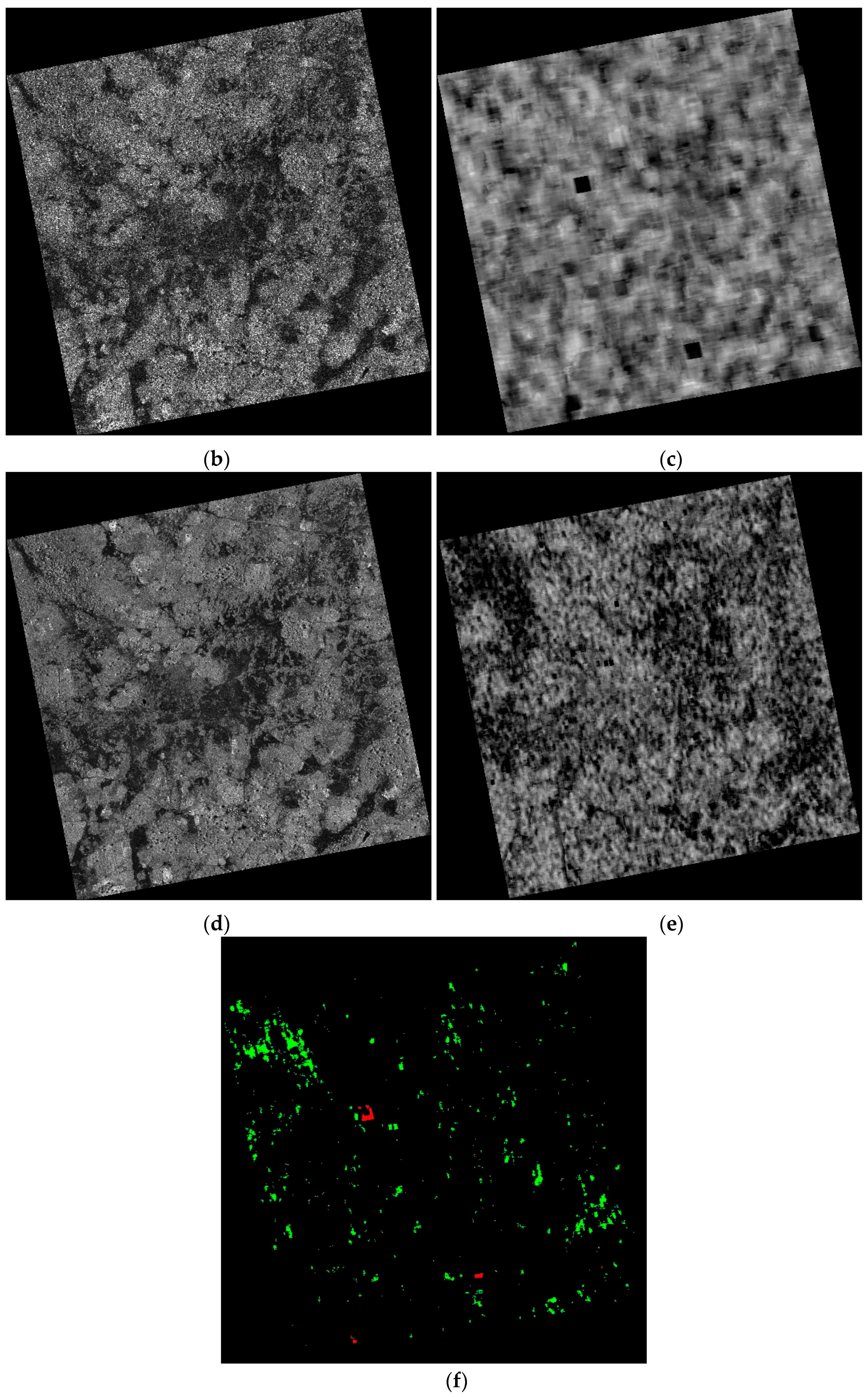
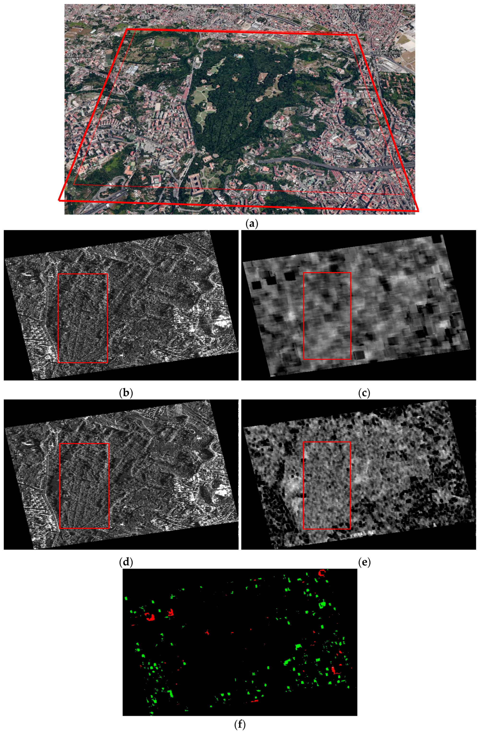
In Figure 5a a Google Earth image of the area of interest is shown (2.3 × 2.3 km2). Also in this case, the optical SPOT image was acquired at the end of Burkina Faso dry season. In Figure 5b,c we present the geocoded stripmap SAR image and the corresponding fractal dimension map, respectively, while in Figure 5d,e the enhanced spotlight SAR image and the corresponding fractal dimension map are shown. Note that, as in the previous case, we applied the geocoding and multilooking procedure described above to the SAR images, and we estimated the fractal maps from the single look SAR images. The same considerations on seasonal variability and on the comparison between the Google Earth and the SAR image hold in this case.
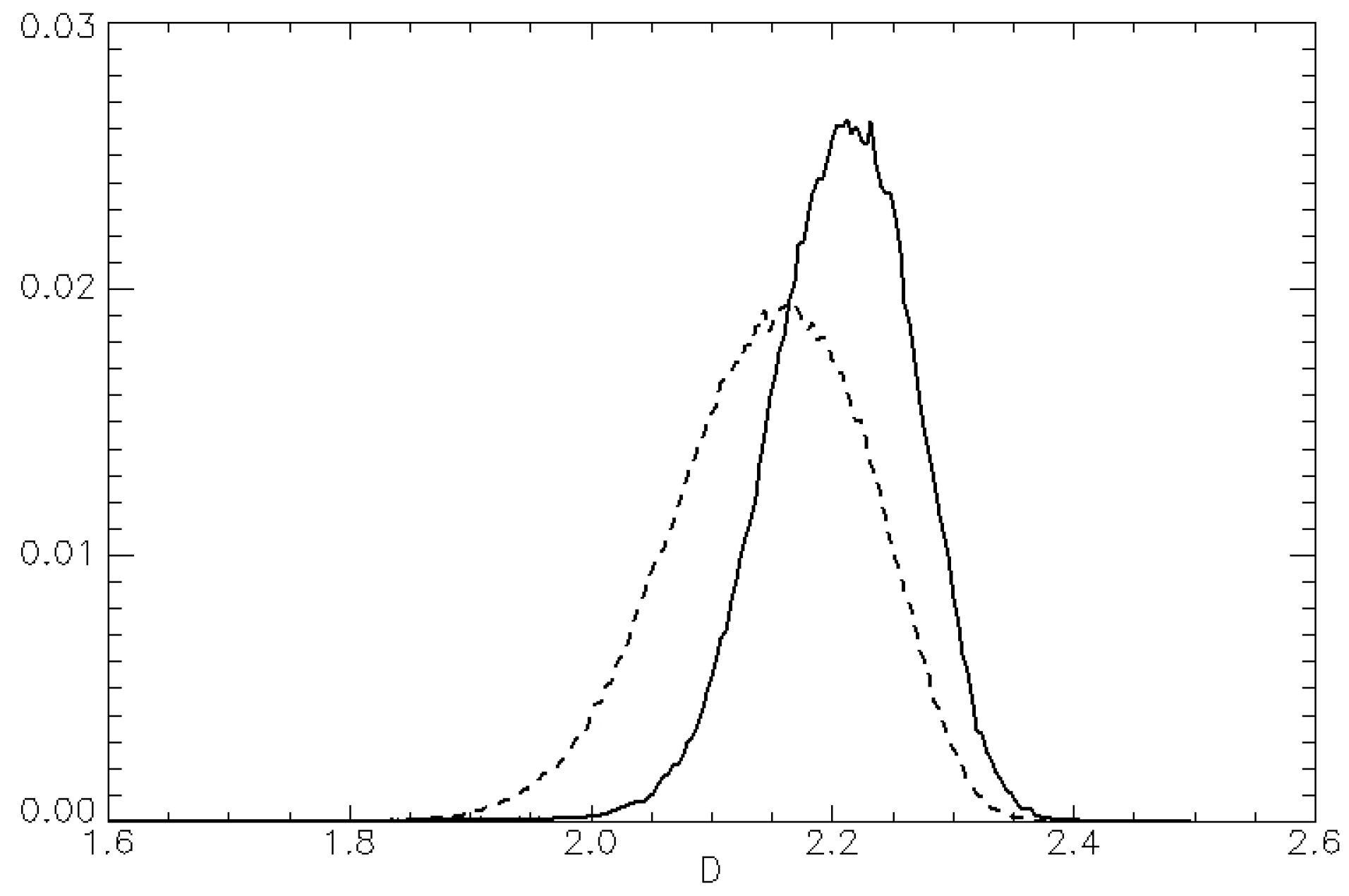
With respect to the images discussed in the previous case, here we can appreciate an increase in vegetated areas and, more in general, the presence of more resolution-scale details. In addition, the image is characterized by the juxtaposition of homogeneous areas of different types (e.g., vegetated and eroded-soil areas), which are responsible for the presence of many edges, i.e., regions of separation between the different areas. The presence of edges allows the testing of the algorithm in the presence of discontinuities, which are one of the critical features for the model validity: in particular, local fractal dimension estimation algorithms behave as edge detectors [17,30], due to the presence within the estimation window of a non-homogeneous texture. Comparing the fractal dimension maps in Figure 5c,e, we can note that the impact of this kind of texture on the map estimated from the spotlight image is significant and it is witnessed by the presence of large areas presenting low values of the fractal dimension (see Figure 5e). This is confirmed by the histograms of the maps in Figure 6 and by the statistics reported in Table 1. In fact, the difference in the average value of the fractal dimension is equal to 0.06, thus being comparable to the standard deviations of both fractal dimension maps.
Very interestingly, the discussed behavior can also be observed on a pixel basis, investigating the joint behavior of the two maps via a feature-based data-fusion technique [37]. In particular, we consider the image obtained by taking the difference of the two geocoded fractal dimension maps, namely the spotlight-based map minus the stripmap-based one. In order to highlight the areas where the two maps present significantly different behavior, in Figure 5f we show a classification map obtained by thresholding the difference image with two thresholds (±0.25): the areas with a difference lower than −0.25 are highlighted in green, while those with a difference greater than 0.25 are red. The areas with a difference in the range [−0.25,0.25] are represented in black. Remembering that very low values of the fractal dimension are obtained in areas close to bright spots, whose presence influences the estimates obtained in an area comparable to the estimation window [30]; we can identify two different mechanisms responsible for the appearance of the two classes. First, the presence of bright spots due to strong trihedral scatterers that are observable on both spot and strip images imply a low fractal dimension on both maps. However, due to the fact that the elaboration windows used to estimate the two maps present the same number of pixels and, hence, a different size in meters, the extension of the low-fractal-dimension area is different in the two maps. This can be observed looking at the red areas in Figure 5f: they usually frame a black area, which is the area interested by the presence of the bright spot, where the fractal dimension is almost the same on the two images. Conversely, the green areas are related to the presence of fine textural details, which are only observable on spotlight images. In particular, in the scene of interest these details are related to the presence of isolated trees.
In summary, as discussed above, the effect of fine-scale (non-fractal) details is more significant on the fractal dimension map obtained from the spotlight image than on the one estimated from the stripmap image and, in this case, this difference emerges in a more evident way.
3.3. Naples 1
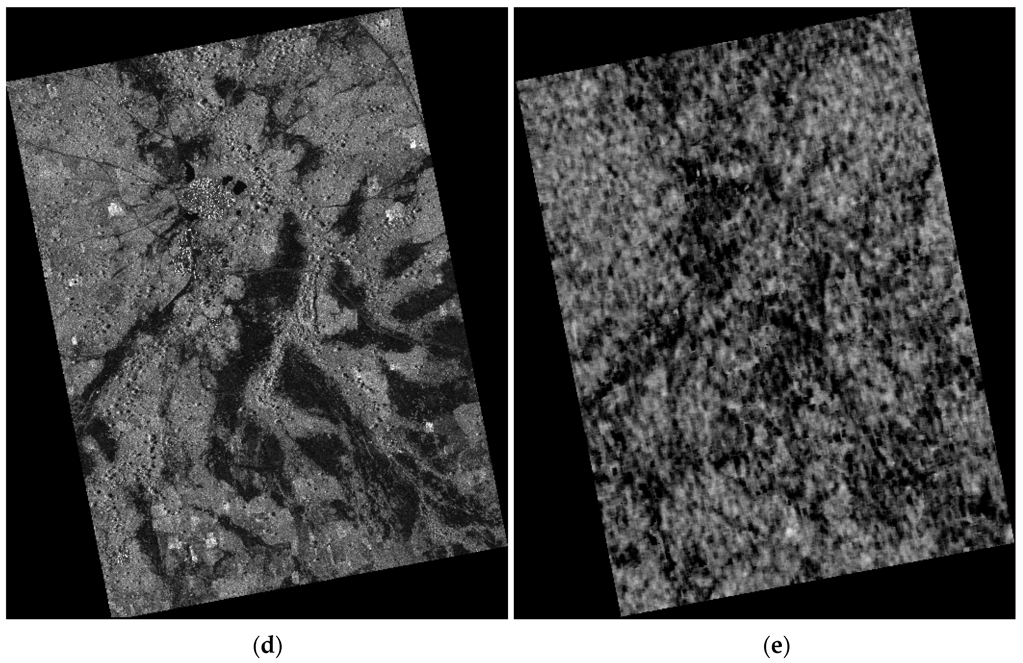
The area of interest in this case is the Bosco di Capodimonte, an urban wood area in the city of Naples, Italy. The Google Earth optical image of the area (2 × 2.7 km2) is shown in Figure 7a. After the application of the same processing used in the previous cases, we obtained the stripmap geocoded image and its corresponding fractal dimension presented in Figure 7b and Figure 7c, respectively, and the enhanced spotlight geocoded image and its associated fractal dimension map shown in Figure 7d,e. Forested areas are frequently used as calibration sites in SAR processing, since they provide very stable values of the reflectivity [38]. We chose this area to test the algorithm behavior over a very homogeneous natural area consisting of closely spaced tall vegetation, rather than of bare soil. Since we are dealing with X-band images, the penetration of the transmitted field under the forest upper-level structure will be very low and the algorithm is supposed to estimate the fractal dimension of the envelope of the treetops.
Looking at the fractal dimension maps in Figure 7c,e, it is evident that the estimated fractal dimension is uniform (i.e., spatially homogeneous) over the forested area, while it presents significant spatial variations in its surroundings. This is due to the presence of man-made objects, whose effect on the estimation algorithm [30] will be better highlighted in the last case study. To avoid the influence of these objects, a subset of the images was considered in the statistical analysis: the considered area is marked in red in Figure 7b–e. In Figure 8 we show the histograms of the fractal dimension maps, while their statistics are reported in Table 1. Actually, the statistical behavior of the two maps is very similar: in particular, the difference in the average values of the fractal dimension is very low with respect to the map’s standard deviations. Therefore, we can conclude that in this case the estimated fractal dimension maps bear essentially the same information.
This can be observed also on the thresholded fractal dimension difference map in Figure 7f (obtained along the same guidelines of the one presented in Figure 4f), where the only relevant differences can be appreciated in the urban areas present on the image. In particular, no significant difference is present on the forested area enclosed in the red box.
3.4. Naples 2
For the last case study, we selected an image of the city of Naples, Italy, covering an area of 2.7 × 2.7 km2 close to the business district and the central station. The Google Earth image of the area is reported in Figure 9a, while in Figure 9b–e the geocoded stripmap and spotlight images and their corresponding fractal dimension maps are shown. In this case, we are interested in studying the behavior of the algorithm over a non-natural area, consisting essentially of buildings and other man-made objects. In this kind of scenario, the fractal models do not hold and the obtained fractal dimension maps present quite large spatial variations.
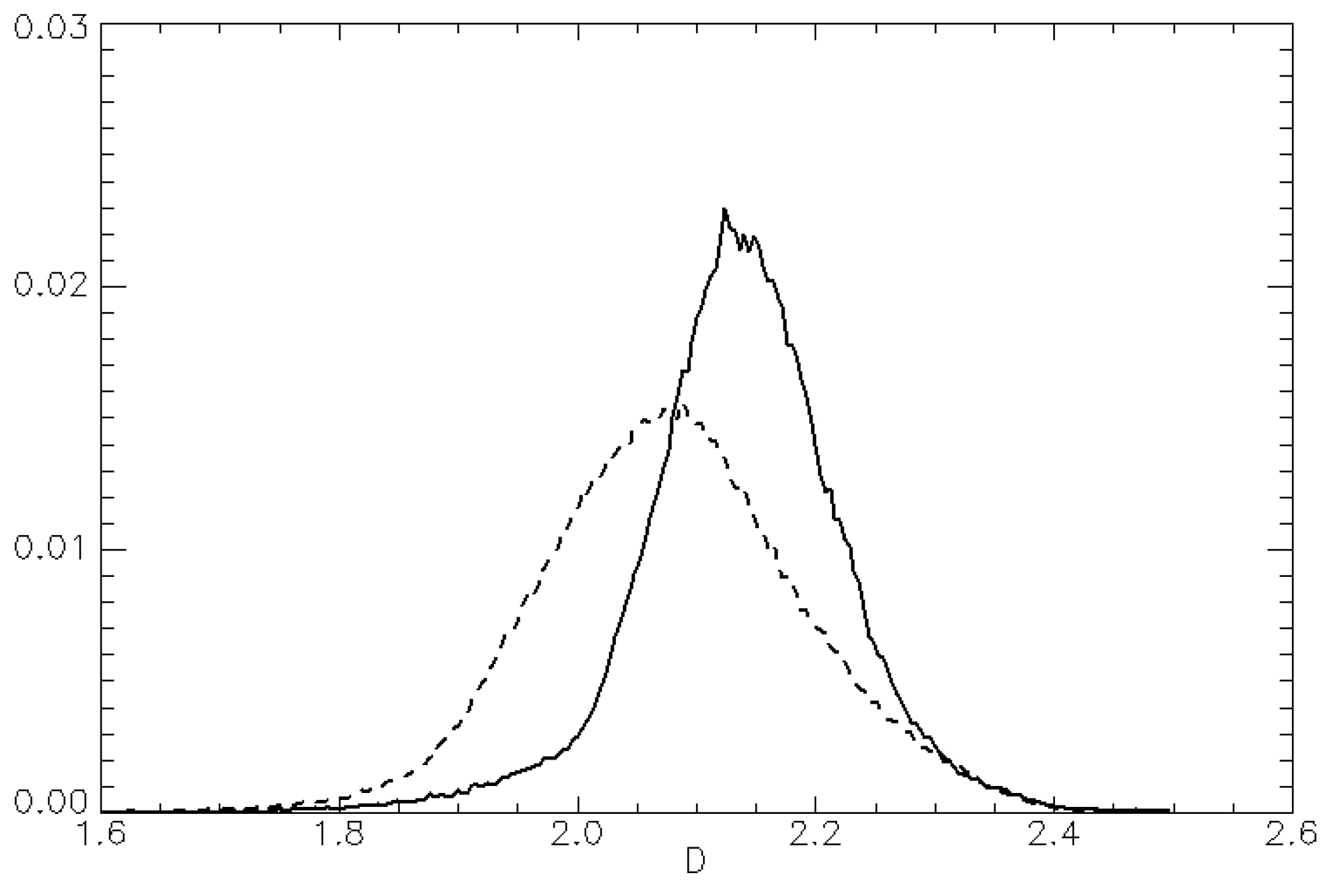
This situation can be considered as a reference for the assessment of similarity of the fractal dimension maps obtained in the previous case studies. In fact, in this case the spotlight acquisition detects much more details than the stripmap, as can be appreciated looking at the high density of dark spots present on the fractal dimension map shown in Figure 9e with respect to the one in Figure 9c. This is also confirmed by the histograms presented in Figure 10 and by the statistics of the maps reported in Table 1. With respect to the previous cases, the standard deviations of the maps are significantly higher and the difference in the average values of the fractal dimension is almost comparable with the standard deviation. In this situation, the thresholded difference mask is not statistically significant, and bears no useful information. Obviously, when applied to man-made areas, that cannot be described through fractal models, the algorithm does not provide values that can be treated as a true fractal dimension of the imaged area. Anyway, these values, though not bearing a precise physical meaning, could provide a valuable support for the identification and characterization of urban areas [30].
4. Conclusions
In this paper we analyzed the behavior of the fractal dimension maps estimated from SAR data acquired using different operational modes. The fractal dimension maps represent the point-by-point fractal dimension of a surface and are estimated from SAR amplitude images. The used data set consists of stripmap and enhanced spotlight Cosmo/SkyMed images collected in the area of Bidi in the North of Burkina Faso and Naples in Italy.
The objective of the work was to highlight potential dependencies of the estimation method on the resolution of the input SAR data. The results of our analysis show that for natural homogeneous areas (e.g., on scarcely vegetated areas and woods) the fractal dimensions estimated from enhanced spotlight and stripmap images are substantially the same; however, estimations from spotlight images are more sensitive to the presence of small objects and sharp edges, which may impair the retrieval of the fractal dimensions performed over areas that include them. Accordingly, when evaluating the fractal dimension of the topography of natural areas is of exclusive interest, it may be more convenient to use stripmap SAR data.
Conversely, in areas containing man-made objects or, more in general, many resolution-scale features (e.g., urban areas), fractal dimension estimates evaluated starting from enhanced spotlight and stripmap images may significantly differ, and, this time, the higher sensitivity to small objects and to man-made typical structures (i.e., buildings, streets, etc.) of fractal dimension maps estimated from spotlight acquisitions is a convenient feature to distinguish and identify such structures. This discussion was also confirmed from the pixel-wise analysis of the image obtained from the difference of the two maps. In this case, we implemented a feature-based data fusion, showing how it is possible to identify meaningful land-cover classes (e.g., trees).
The presented results provide a new basis for the development of further data fusion techniques based on the combined use of multi-operational data. In fact, the combination of fractal dimension values obtained from stripmap and spotlight data is not trivial, and should be based not simply on the classical trade-off between coverage and resolution, but also on the specific application. In general, if we are interested in obtaining a reliable estimate of the fractal dimension of the observed natural scene, stripmap images should be chosen in view of economic and computational considerations (stripmap data are significantly less expensive than spotlight data and the number of samples for equal sized areas is lower). In turn, the combination of fractal dimension maps obtained from stripmap and spotlight images can be used to identify areas on the scene presenting non-fractal behavior (e.g., urban areas).
Acknowledgments
The images were provided by ASI in the framework of two Cosmo-SkyMed 2007 AO projects: Project 1200 “Exploitation of fractal scattering models for COSMO-SkyMed images interpretation,” and Project 2218 “Use of high resolution SAR data for water resource management in semi-arid regions.”
Author Contributions
All the authors equally contributed to the conceiving, writing, and experiments of the work.
Conflicts of Interest
The authors declare no conflict of interest.
References
- Mandelbrot, B.B. The Fractal Geometry of Nature; Freeman: New York, NY, USA, 1983. [Google Scholar]
- Franceschetti, G.; Riccio, D. Scattering, Natural Surfaces and Fractals; Academic Press: Burlington, VT, USA, 2007. [Google Scholar]
- Falconer, K. Fractal Geometry; Wiley: Chichester, UK, 1989. [Google Scholar]
- Feder, J.S. Fractals; Plenum: New York, NY, USA, 1988. [Google Scholar]
- Turcotte, D.L. Fractals and Chaos in Geology and Geophysics; Cambridge University Press: Cambridge, UK, 1997. [Google Scholar]
- Campbell, B.A. Scale-dependent surface roughness behavior and its impact on empirical models for radar backscatter. IEEE Trans. Geosci. Remote Sens. 2009, 47, 3480–3488. [Google Scholar] [CrossRef]
- Dierking, W. Quantitative Roughness Characterization of Geological Surfaces and Implications for Radar Signature Analysis. IEEE Trans. Geosci. Remote Sens. 1999, 37, 2397–2412. [Google Scholar] [CrossRef] [Green Version]
- Shepard, M.K.; Campbell, B.A.; Bulmer, M.H.; Farr, T.G.; Gaddis, L.R.; Plaut, J.J. The roughness of natural terrain: A planetary and remote sensing perspective. J. Geophys. Res. 2001, 106, 32777–32795. [Google Scholar] [CrossRef]
- Gaddis, L.R.; Mouginis-Mark, P.J.; Hayashi, J.N. Lava flow surface textures: SIR-B radar image texture, field observations, and terrain measurements. Photogramm. Eng. Remote Sens. 1990, 56, 211–224. [Google Scholar]
- Austin, T.; England, A.W.; Wakefield, G.H. Special problems in the estimation of power-law spectra as applied to topographical modeling. IEEE Trans. Geosci. Remote Sens. 1994, 32, 928–939. [Google Scholar] [CrossRef]
- Di Martino, G.; Iodice, A.; Riccio, D.; Ruello, G. Equivalent number of scatterers for SAR speckle modeling. IEEE Trans. Geosci. Remote Sens. 2014, 52, 2555–2564. [Google Scholar] [CrossRef]
- Franceschetti, G.; Callahan, P.S.; Iodice, A.; Riccio, D.; Wall, S.D. Titan, Fractals, and Filtering of Cassini Altimeter Data. IEEE Trans. Geosci. Remote Sens. 2006, 44, 2055–2062. [Google Scholar] [CrossRef]
- Pesquet-Popescu, B.; Véhel, J.L. Stochastic fractal models for image processing. IEEE Signal Process. Mag. 2002, 19, 48–62. [Google Scholar] [CrossRef]
- Stewart, C.V.; Moghaddam, B.; Hintz, K.J.; Novak, L.M. Fractional Brownian Motion Models for Synthetic Aperture Radar Imagery Scene Segmentation. Proc. IEEE 1993, 81, 1511–1522. [Google Scholar] [CrossRef]
- Kaplan, L.M. Extended Fractal Analysis for Texture Classification and Segmentation. IEEE Trans. Image Process. 1999, 8, 1572–1585. [Google Scholar] [CrossRef] [PubMed]
- Jansing, E.D.; Chenoweth, D.L.; Knecht, J. Feature detection in synthetic aperture radar images using fractal error. In Proceedings of the IEEE Aerospace Conference, Aspen, CO, USA, 13 February 1997; pp. 187–195. [Google Scholar]
- Jansing, E.D.; Allen, B.; Chenoweth, D.L. Edge enhancement using the fractal error metric. In Proceedings of the 1st International Conference on Engineering Design and Automation, Bangkok, Thailand, 18–21 March 1997. [Google Scholar]
- Pentland, A.P. Fractal-Based Description of Natural Scenes. IEEE Trans. Pattern Anal. Mach. Intell. 1984, 6, 661–674. [Google Scholar] [CrossRef] [PubMed]
- Kube, P.; Pentland, A. On the imaging of fractal surfaces. IEEE Trans. Pattern Anal. Mach. Intell. 1988, 10, 704–707. [Google Scholar] [CrossRef]
- Korvin, G. Is the optical image of a non-Lambertian fractal surface fractal? IEEE Geosci. Remote Sens. Lett. 2005, 2, 380–383. [Google Scholar] [CrossRef]
- Di Martino, G.; Iodice, A.; Riccio, D.; Ruello, G. Imaging of Fractal Profiles. IEEE Trans. Geosci. Remote Sens. 2010, 48, 3280–3289. [Google Scholar] [CrossRef]
- Di Martino, G.; Riccio, D.; Zinno, I. SAR Imaging of Fractal Surfaces. IEEE Trans. Geosci. Remote Sens. 2012, 50, 630–644. [Google Scholar] [CrossRef]
- Danudirdjo, D.; Hirose, A. Local Subpixel Coregistration of Interferometric Synthetic Aperture Radar Images Based on Fractal Models. IEEE Trans. Geosci. Remote Sens. 2013, 51, 4292–4301. [Google Scholar] [CrossRef]
- Danudirdjo, D.; Hirose, A. InSAR Image Regularization and DEM Error Correction with Fractal Surface Scattering Model. IEEE Trans. Geosci. Remote Sens. 2015, 53, 1427–1439. [Google Scholar] [CrossRef]
- Danudirdjo, D.; Hirose, A. Anisotropic Phase Unwrapping for Synthetic Aperture Radar Interferometry. IEEE Trans. Geosci. Remote Sens. 2015, 53, 4116–4126. [Google Scholar] [CrossRef]
- Di Martino, G.; Di Simone, A.; Iodice, A.; Riccio, D. Scattering-Based Nonlocal Means SAR Despeckling. IEEE Trans. Geosci. Remote Sens. 2016, 54, 3574–3588. [Google Scholar] [CrossRef]
- Di Martino, G.; Di Simone, A.; Iodice, A.; Poggi, G.; Riccio, D.; Verdoliva, L. Scattering-Based SARBM3D. IEEE J. Sel. Top. Appl. Earth Obs. Remote Sens. 2016, 9, 2131–2144. [Google Scholar] [CrossRef]
- Di Martino, G.; Iodice, A.; Riccio, D.; Ruello, G.; Zinno, I. Angle Independence Properties of Fractal Dimension Maps Estimated from SAR Data. IEEE J. Sel. Top. Appl. Earth Obs. Remote Sens. 2013, 6, 1242–1253. [Google Scholar] [CrossRef]
- Di Martino, G.; Iodice, A.; Riccio, D.; Ruello, G.; Zinno, I. The effects of polarization on fractal dimension maps estimated from SAR data. In Proceedings of the PolInSAR 2013 (ESA SP-713), Frascati, Italy, 28 January–1 February 2013. [Google Scholar]
- Di Martino, G.; Iodice, A.; Riccio, D.; Ruello, G.; Zinno, I. Fractal Filtering Applied to SAR Images of Urban Areas. In Proceedings of the Urban Remote Sensing Event JURSE, Munich, Germany, 11–13 April 2011. [Google Scholar]
- Capon, J. High-Resolution Frequency-Wavenumber Spectrum Analysis. Proc. IEEE 1969, 57, 1408–1418. [Google Scholar] [CrossRef]
- Kay, S.M. Modern Spectral Analysis; Patience Hall: Englewood Cliffs, NJ, USA, 1999. [Google Scholar]
- Amitrano, D.; Di Martino, G.; Iodice, A.; Riccio, D.; Ruello, G.; Ciervo, F.; Papa, M.N.; Koussoube, Y. Effectiveness of high-resolution SAR for water resource management in low-income semi-arid countries. Int. J. Remote Sens. 2014, 35, 70–88. [Google Scholar] [CrossRef]
- Amitrano, D.; Di Martino, G.; Iodice, A.; Riccio, D.; Ruello, G. A New Framework for SAR Multitemporal Data RGB Representation: Rationale and Products. IEEE Trans. Geosci. Remote Sens. 2015, 53, 117–133. [Google Scholar] [CrossRef]
- Di Martino, G.; Poderico, M.; Poggi, G.; Riccio, D.; Verdoliva, L. Benchmarking Framework for SAR Despeckling. IEEE Trans. Geosci. Remote Sens. 2014, 52, 1596–1615. [Google Scholar] [CrossRef]
- Di Martino, G.; Poggi, G.; Riccio, D.; Verdoliva, L. Effects of Despeckling on the Estimation of Fractal Dimension from SAR Images. In Proceedings of the IEEE International Geoscience and Remote Sensing Symposium, Melbourne, Australia, 21–26 July 2013; pp. 3950–3953. [Google Scholar]
- Pohl, C.; Van Genderen, J.L. Multisensor image fusion in remote sensing: Concepts, methods and applications. Int. J. Remote Sens. 1998, 19, 823–854. [Google Scholar] [CrossRef]
- Freeman, A. SAR calibration: An overview. IEEE Trans. Geosci. Remote Sens. 1992, 30, 1107–1121. [Google Scholar] [CrossRef]
Figure 1.
Flow chart of the processing used for the estimation of the fractal dimension within the sliding window.
Figure 1.
Flow chart of the processing used for the estimation of the fractal dimension within the sliding window.

Figure 2.
(a) Google Earth view of the subset Burkina 1, with the footprint of the imaged area of interest marked in red; (b) geocoded stripmap acquisition; (c) fractal dimension map corresponding to (b); (d) geocoded enhanced spotlight image; (e) fractal dimension map corresponding to (d).
Figure 2.
(a) Google Earth view of the subset Burkina 1, with the footprint of the imaged area of interest marked in red; (b) geocoded stripmap acquisition; (c) fractal dimension map corresponding to (b); (d) geocoded enhanced spotlight image; (e) fractal dimension map corresponding to (d).
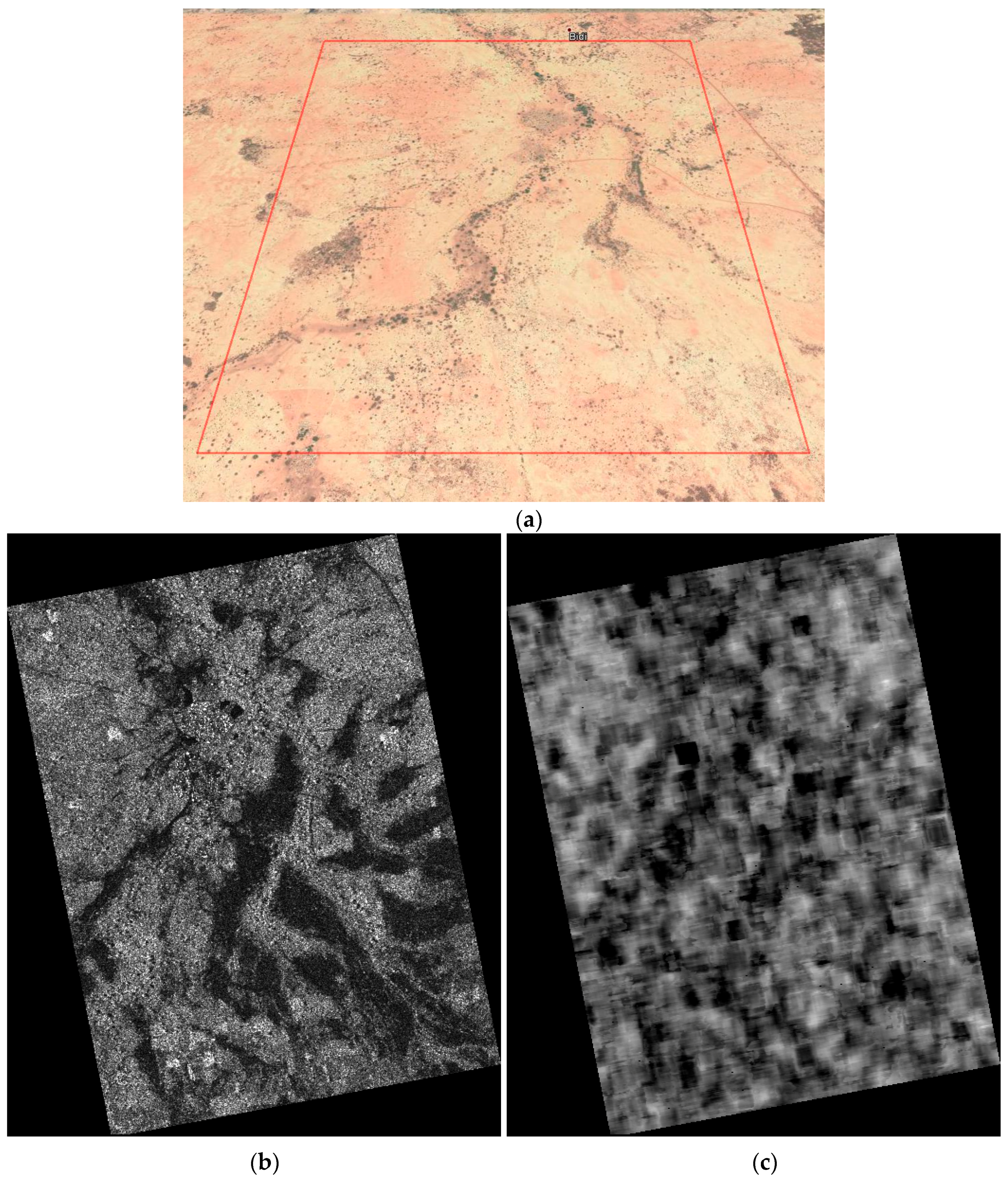

Figure 3.
Histogram of the fractal dimension maps of Figure 2c,e: solid line for the stripmap and dashed line for the enhanced spotlight.
Figure 3.
Histogram of the fractal dimension maps of Figure 2c,e: solid line for the stripmap and dashed line for the enhanced spotlight.
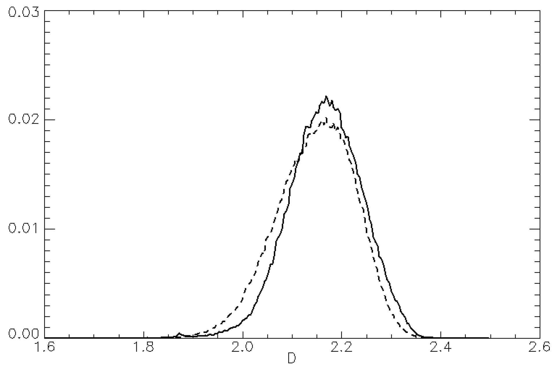
Figure 4.
Histogram of the fractal dimension map of Figure 2c compared to that of the fractal dimension map obtained from enhanced spotlight 3 × 3 multilook data: solid line for the stripmap and dashed line for the multilook enhanced spotlight.
Figure 4.
Histogram of the fractal dimension map of Figure 2c compared to that of the fractal dimension map obtained from enhanced spotlight 3 × 3 multilook data: solid line for the stripmap and dashed line for the multilook enhanced spotlight.

Figure 5.
(a) Google Earth view of the subset Burkina 2, with the footprint of the imaged area of interest marked in red; (b) geocoded stripmap acquisition; (c) fractal dimension map corresponding to (b); (d) geocoded enhanced spotlight image; (e) fractal dimension map corresponding to (d); (f) thresholded difference map.


Figure 6.
Histogram of the fractal dimension maps of Figure 4c,e: solid line for the stripmap and dashed line for the enhanced spotlight.
Figure 6.
Histogram of the fractal dimension maps of Figure 4c,e: solid line for the stripmap and dashed line for the enhanced spotlight.

Figure 7.
(a) Google Earth view of the subset Naples 1, with the footprint of the imaged area of interest marked in red; (b) geocoded stripmap acquisition; (c) fractal dimension map corresponding to (b); (d) geocoded enhanced spotlight image; (e) fractal dimension map corresponding to (d); (f) thresholded difference map.

Figure 8.
Histogram of the fractal dimension maps of Figure 7c,e: solid line for the stripmap and dashed line for the enhanced spotlight.
Figure 8.
Histogram of the fractal dimension maps of Figure 7c,e: solid line for the stripmap and dashed line for the enhanced spotlight.
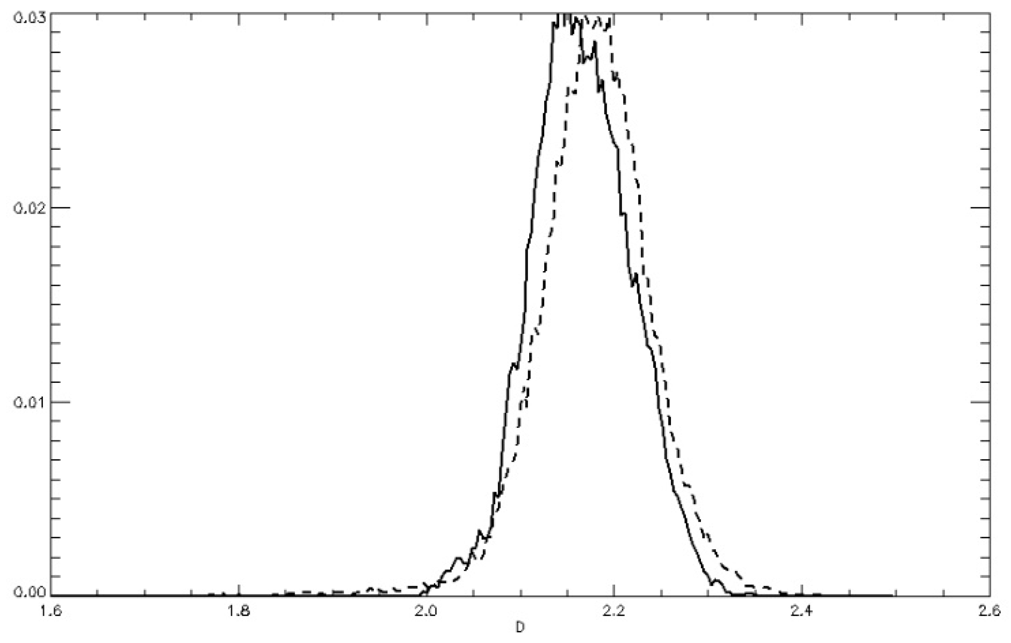
Figure 9.
(a) Google Earth view of the subset Naples 2, with the footprint of the imaged area of interest marked in red; (b) geocoded stripmap acquisition; (c) fractal dimension map corresponding to (b); (d) geocoded enhanced spotlight image; (e) fractal dimension map corresponding to (d).
Figure 9.
(a) Google Earth view of the subset Naples 2, with the footprint of the imaged area of interest marked in red; (b) geocoded stripmap acquisition; (c) fractal dimension map corresponding to (b); (d) geocoded enhanced spotlight image; (e) fractal dimension map corresponding to (d).
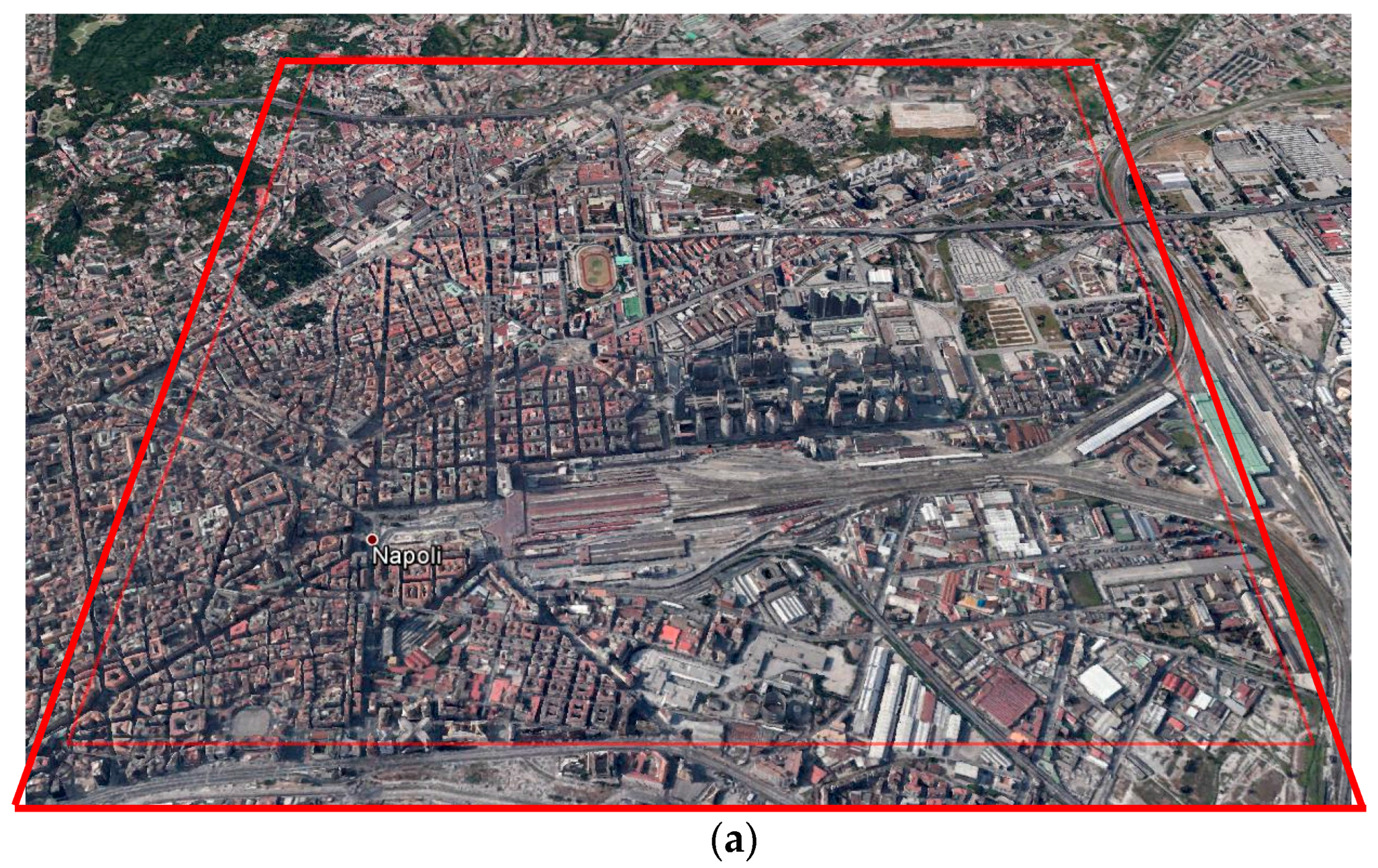
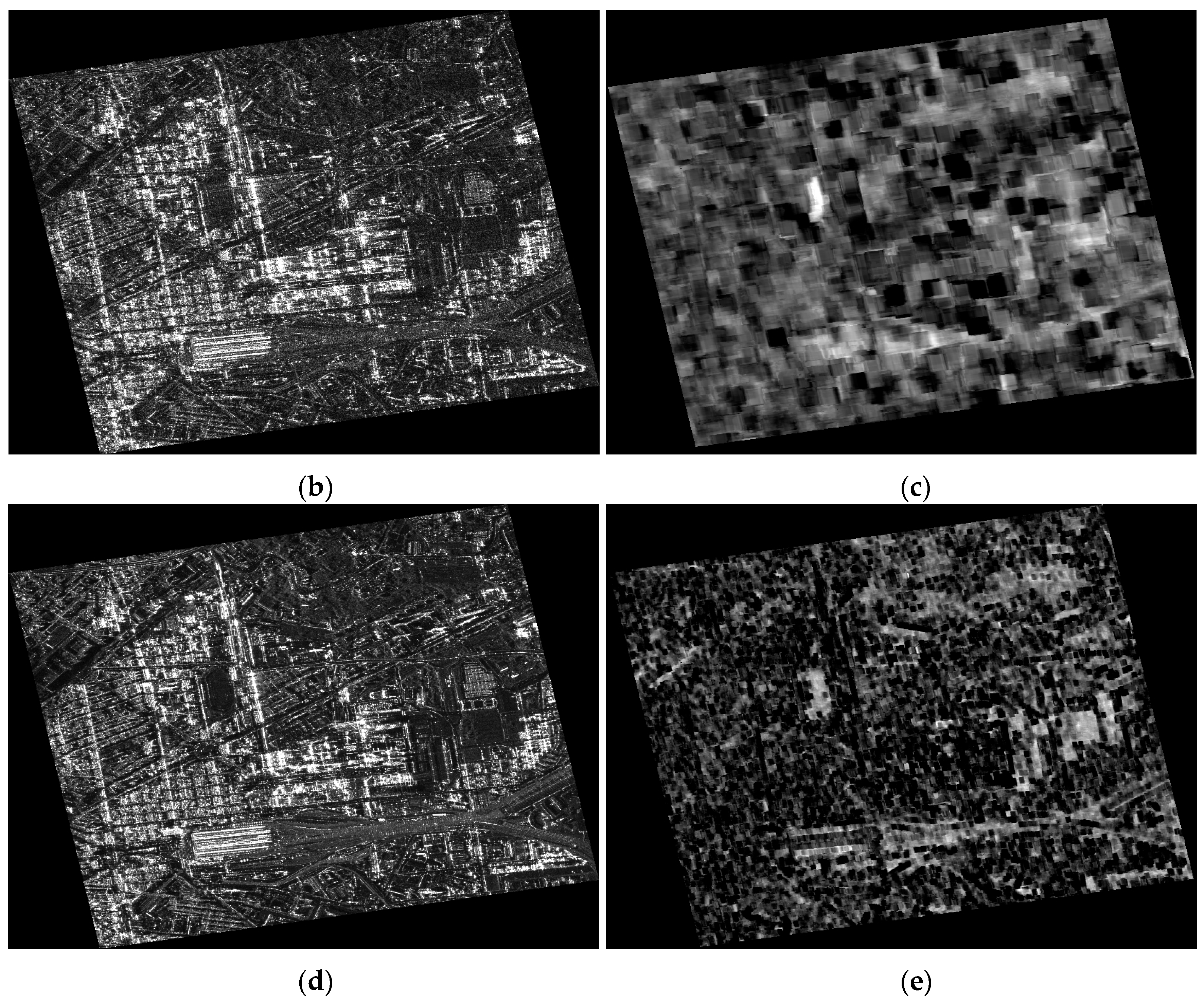
Figure 10.
Histogram of the fractal dimension maps of Figure 9c,e: solid line for the stripmap and dashed line for the enhanced spotlight.
Figure 10.
Histogram of the fractal dimension maps of Figure 9c,e: solid line for the stripmap and dashed line for the enhanced spotlight.

Table 1.
Statistics of the subsets.
| Subset | Mode | Dmean | Dstdev |
|---|---|---|---|
| Burkina 1 | Strip | 2.17 | 0.07 |
| Spot | 2.15 | 0.08 | |
| Burkina 2 | Strip | 2.21 | 0.06 |
| Spot | 2.15 | 0.08 | |
| Naples 1 | Strip | 2.17 | 0.05 |
| Spot | 2.18 | 0.06 | |
| Naples 2 | Strip | 2.14 | 0.09 |
| Spot | 2.08 | 0.11 |
© 2017 by the authors. Licensee MDPI, Basel, Switzerland. This article is an open access article distributed under the terms and conditions of the Creative Commons Attribution (CC BY) license (http://creativecommons.org/licenses/by/4.0/).
Share and Cite
MDPI and ACS Style
Di Martino, G.; Iodice, A.; Riccio, D.; Ruello, G.; Zinno, I. The Role of Resolution in the Estimation of Fractal Dimension Maps From SAR Data. Remote Sens. 2018, 10, 9. https://doi.org/10.3390/rs10010009
AMA Style
Di Martino G, Iodice A, Riccio D, Ruello G, Zinno I. The Role of Resolution in the Estimation of Fractal Dimension Maps From SAR Data. Remote Sensing. 2018; 10(1):9. https://doi.org/10.3390/rs10010009
Chicago/Turabian StyleDi Martino, Gerardo, Antonio Iodice, Daniele Riccio, Giuseppe Ruello, and Ivana Zinno. 2018. "The Role of Resolution in the Estimation of Fractal Dimension Maps From SAR Data" Remote Sensing 10, no. 1: 9. https://doi.org/10.3390/rs10010009
Note that from the first issue of 2016, this journal uses article numbers instead of page numbers. See further details here.