Correction of Pushbroom Satellite Imagery Interior Distortions Independent of Ground Control Points


1
State Key Laboratory of Information Engineering in Surveying, Mapping and Remote Sensing, Wuhan University, Wuhan 430079, China
2
Collaborative Innovation Center of Geospatial Technology, Wuhan University, Wuhan 430079, China
3
China Academy of Space Technology, Beijing 100094, China
*
Author to whom correspondence should be addressed.
†
These authors contributed equally to this work.
Remote Sens. 2018, 10(1), 98; https://doi.org/10.3390/rs10010098
Submission received: 28 October 2017
/
Revised: 9 January 2018
/
Accepted: 10 January 2018
/
Published: 12 January 2018
(This article belongs to the Section Remote Sensing Image Processing)
Abstract
:Compensating for distortions in pushbroom satellite imagery has a bearing on subsequent earth observation applications. Traditional distortion correction methods usually depend on ground control points (GCPs) acquired from a high-accuracy geometric calibration field (GCF). Due to the high construction costs and site constraints of GCF, it is difficult to perform distortion detection regularly. To solve this problem, distortion detection methods without using GCPs have been proposed, but their application is restricted by rigorous conditions, such as demanding a large amount of calculation or good satellite agility which are not met by most remote sensing satellites. This paper proposes a novel method to correct interior distortions of satellite imagery independent of GCPs. First, a classic geometric calibration method for pushbroom satellite is built and at least three images with overlapping areas are collected, then the forward intersection residual between corresponding points in the images are used to calculate interior distortions. Experiments using the Gaofen-1 (GF-1) wide-field view-1 (WFV-1) sensor demonstrate that the proposed method can increase the level of orientation accuracy from several pixels to within one pixel, thereby almost eliminating interior distortions. Compared with the orientation accuracy by classic GCF method, there exists maximum difference of approximately 0.4 pixel, and the reasons for this discrepancy are analyzed. Generally, this method could be a supplementary method to conventional methods to detect and correct the interior distortion.
1. Introduction
Interior distortions of pushbroom satellite images are mostly caused by camera lens aberrations, and results in nonlinear geo-positioning errors that are difficult to eliminate in practical applications with few ground control points (GCPs). Obtaining higher geo-positioning accuracy through the detection and compensation of interior distortions is crucial for improving the performance and potential of satellite images. This also has a bearing on subsequent earth observation applications, such as ortho-rectification, digital elevation model (DEM) generation [1,2], or surface change detection. Consequently, it is critical to detect and correct interior distortion of satellite images.
Several methods have been proposed to correct interior distortions in pushbroom satellite images. With its high accuracy and computational stability, the classical method using a geometric calibration field (GCF) to calibrate image distortion is undoubtedly the most common method [3,4,5]. GCF is composed of a sub-meter or sub-decimeter digital orthophoto map (DOM) and DEM model that are obtained from aerial photogrammetry and cover a certain area. Every pixel in the GCF can be regarded as a high-precision GCP. When a satellite passes over the GCF, numerous GCPs can be acquired from the GCF in order to detect and correct image distortion [6]. The core problem of this classical method is the high-precision registration between the acquired image and the DOM. Bouillon [4] proposed a simulation-registration strategy to acquire a large number of GCPs, which is successfully used in the calibration of SPOT-5. Leprince et al. [3,7] improved the method by creating a high-precision phase correlation algorithm to obtain GCPs pixel by pixel. To reduce the calculation burden, Zhang [8] and Jiang et al. [9] recommended extracting feature points before high-precision registration.
Although the classical method is easy and stable, it requires a costly update of aerial imagery and there is a lot of geometric work such as acquiring high-precision GCPs and performing aerial triangulation of all aerial images for establishing new GCF. On one hand, the presence of temporary objects such as new construction sites, as well as other changes in the environment that occur between obtaining the satellite image and GCF images—caused by long acquisition intervals—affects the effectiveness of the GCF method. On the other hand, restricted by the revisit period of satellite and bad weather, the satellite images of GCF sometimes cannot be acquired timely to perform geometric calibration. Furthermore, as image swaths become wider than current GCF, it is difficult to implement conventional GCF. In other words, it is difficult to obtain sufficient GCPs from current GCFs to solve the calibration parameters of all rows in one image of wide swath. Take the GF-1 WFV camera as an example, hereunder Table 1 shows currently available GCFs in China that fail to cover all rows in one GF-1 WFV image which spans 200 km. To address this problem, a multi-calibration image strategy and a modified calibration model have been proposed [6], whereby calibration images are collected at different times, and their different rows are covered by the GCF. GCPs covering all rows can then be obtained, and a modified calibration model can be applied to detect distortions. Nevertheless, this method depends heavily on the distribution of images and GCF, and mosaicking between images should be handled carefully in the modified classic GCF model. Consequently, it is difficult for imagery vendors to perform regularly distortion detection. Distortion detection methods independent of GCPs have thus been explored.
Self-calibration block adjustment [10,11,12,13,14,15] is one feasible method independent of GCF, and it can be used to compensate for distortion. Self-calibration adjustment takes additional parameters (such as distortion parameters), which are calculated together with the block adjustment parameters, into consideration in the block adjustment. However, the process demands collection of a large number of images, and it focuses on the calculation of block adjustment parameters. In addition, it requires a large amount of calculation, and performs best with some GCPs to provide more reasonable results. Pleiades-HR satellites provide another novel solution independent of GCF called geometric auto-calibration that addresses limitations of other methods [16,17,18]. Relying on good satellite agility, Pleiades can obtain two images with a crossing angle of about 90 degrees. In practice, one image is re-sampled into the other with available accurate geometric models and DEM [19], by which the two images are correlated. Then, statistical computation is applied on lines and columns to reflect the distortion and attitude high frequency residues. The method can detect distortion and partly compensates for the disadvantages of GCF-based methods. However, it can only be implemented with satellites characterized by good agility and only if a corresponding DEM exists.
In the computer vision (CV) field, Faugeras et al. [20] and Hartley [21] proposed an auto-calibration technique and proved that it is possible to directly detect the distortion from multi images. In addition, Malis [22,23] inherited the thought, and advised to conduct auto-calibration from unknown planar structures of multi images, which achieves relatively good results in the experiments. However, this method was only used in close-range photogrammetry or computer vision, and has not been applied in the satellite photogrammetry yet, especially in the wide swath satellite image. When the method is used in satellite photogrammetry, several problems should be resolved: it is impossible to acquire planar structures for satellite imagery because of the influence of the earth’s curvature, especially for the wide swath imagery; the method needs to solve nonlinear equations by massive computations, and the process is often unstable.
Some conditions, such as an appropriate GCF, the number of images required, and calculation burden, are difficult for imagery vendors to meet. Others, such as satellite agility, are hard to satisfy for most remote sensing satellites. In this paper, a novel method is proposed to detect interior distortions of a pushbroom satellite image independent of GCPs. This method uses at least three images with overlapping areas, and takes advantage of the forward intersection residual between corresponding points in these images to detect interior distortions. Compared with traditional methods implemented by GCF or that depend on satellite agility, the proposed method is free from these constraints and it can correct interior distortions of images of any terrain. We present experiments using the Gaofen-1 (GF-1) wide-field view-1 (WFV-1) sensor to verify the accuracy of the proposed method. Compared with traditional methods that are implemented by GCF or that depend on satellite agility, the proposed method is free from these constraints and can work for any terrain and improve the internal geometric quality of satellite imagery.
2. Materials and Methods
2.1. Fundamental Theory
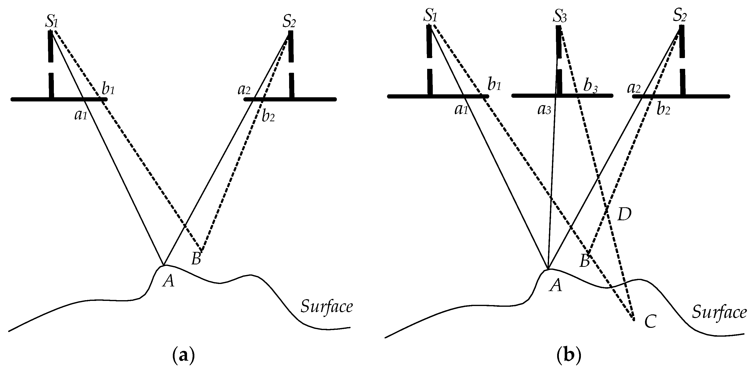
The fundamental theory of interior distortion detection independent of GCPs is shown in Figure 1. In Figure 1a, there are two images, and S1 and S2 are the projection centers of the two images respectively. The thick solid lines a1b1 and a2b2 represent the focal planes of the two images. The irregular curve represents the real ground surface, and point A is a ground point on the surface. Without any error, point A projects to image S1 at a1, and projects to image S2 at a2. The forward intersection point between S1 and S2 is A. a1 and a2 are the corresponding image points of A in images S1 and S2. However, if image distortion exists, the image coordinate a1 is moved to b1, and a2 is moved to b2. The dotted lines S1b1 and S2b2 are the new lines of sight, and the new forward intersection point is B. In short, image distortions result in changes in image coordinates, and indirectly cause a change in the ground point.
However, if the position of ground surface point A is unknown, Figure 1a can also conversely be interpreted to show that the position error of the ground point leads to a change in the image coordinate. Two images are insufficient to determine whether the change in image coordinate is caused by image distortion or ground point error. Therefore, two images are insufficient to detect image distortion.
A third image S3 is introduced to solve this problem, as shown in Figure 1b. Without any error, point A projects to image S3 at a3. However, due to errors, the image coordinate a3 is moved to b3. The dotted line S3b3 is the new line of sight, and the new forward intersection point is C with S1, and D with S2. If the change in image coordinate is caused by ground point error, then the forward intersection points B, C, and D should be exactly the same. If the change in image coordinate is caused by image distortion, then the forward intersection values B, C, and D may be different. We call this difference the forward intersection residual.
Through the above analysis, the forward intersection residual between the corresponding points of three images can be used as a distortion evaluation criterion. Distortion can be detected by constraining the forward intersection residual to the minimum, after it which the adjustment equation for distortion parameters can be built and calculated.
2.2. Distortion Detection Method
2.2.1. Calibration Model
The calibration model for the linear sensor model is established based on Tang et al. [24] and Xu et al. [25] as Equation (1):
where indicates satellite position with respect to the geocentric Cartesian coordinate system, and R(t) is the rotation matrix converting the body coordinate system to the geocentric Cartesian coordinate system. Both these parameters are functions of time t. Here, represents the ray direction, whose z-coordinate is a constant with a value of 1 in the body coordinate system. Furthermore, m denotes the unknown scaling factor and is the ground position of the pixel in the geocentric Cartesian coordinate system. RU is the offset matrix that compensates for exterior errors, and denotes interior distortions in the image space.
RU can be expanded by introducing variables [26,27,28]:
where ω, ϕ and κ are rotations about the X, Y, and Z axes of the satellite body coordinate, respectively, and should be detected in order to eliminate exterior errors. With images collected at different times having different exterior errors, it is noted that there is a corresponding RU for each image.
Considering that the highest order term of distortion is 5, a classic polynomial model to describe distortions (Δx, Δy) can be written as follows [9,25,29,30,31]:
where variables , and are parameters describing distortion, and s is the image coordinate across track. Images collected at different times have the same distortion.
Based on Equations (1)–(3), the calibration model can be written as Equation (4) for a specified image:
where ω, ϕ, Κ, , and are parameters. Unlike the classical method, variable [Xs, Ys, Zs] in Equation (4) is the unknown ground position in the proposed method, which should be adjusted by the distortion detection method.
Equation (4) can be rewritten in image form as Equation (5):
Equation (5) is the basic calibration model of the proposed method.
2.2.2. Distortion Detection Method
Taking the partial derivative of Equation (5) for , , ω, ϕ, Κ, and [Xs, Ys, Zs], the linearized form of Equation (5) can be expressed as error Equation (6) for object point k projected in image j:
where v is the discrepancy of error equation, l is the error vector calculated by current calibration paramters, x is the number of image column and y is the number of image line.
As mentioned above, distortion can be detected by constraining the forward intersection residual to a minimum. Equation (6) implicitly uses this condition by giving the same object value to corresponding points in different images. For convenience, error Equation (6) can be simplified into Equation (7):
where is the correction to the calibration parameters of image j, and represents the correction to the object coordinates of object point k.
Considering different images and different object points, the error equation can be written as Equation (8):
where m is the number of images (m > 2), and n represents the number of GCPs intersected by corresponding points between images.
For convenience, Equation (8) can be simplified to Equation (9):
where represents correction to the image calibration parameters, and represents correction to the object coordinates of the unknown object points. A and B are coefficient matrices in the error equation, and L is the constant vector. Equation (9) is the basic error equation of our proposed method.
2.2.3. Solution of Error Equations
Equation (9) is the basic error equation, and the corresponding normal equation of (9) is Equation (10):
which can be simplified to Equation (11):
If there are several unknown object points (because many corresponding points can be detected between images by the proposed method), the number of error equations will be huge, and the rank of Equation (11) will also be striking. In this case, calculation would be time-consuming. Moreover, it is unnecessary to calculate the unknown correction to object coordinates X when the proposed method is used. In order to solve this problem, the reduced normal equation yielded by eliminating one type of parameter can be used. The reduced normal equation for correction to calibration parameters, t, from normal Equation (11) is Equation (12):
The reduced normal equation may be in a poor state, because of correlation between calibration parameters. To solve this problem, we use iteration by correcting characteristic value (ICCV) [32], which can be applied to many situations, such as morbidity or loss of rank, to calculate the equation.
After correction to calibration parameters, t, is calculated, the calibration parameters can be updated and the coordinates of the object points can be acquired by the forward intersection.
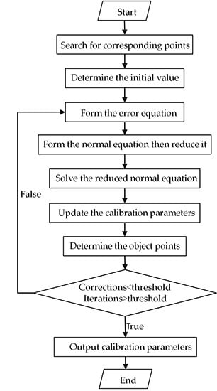
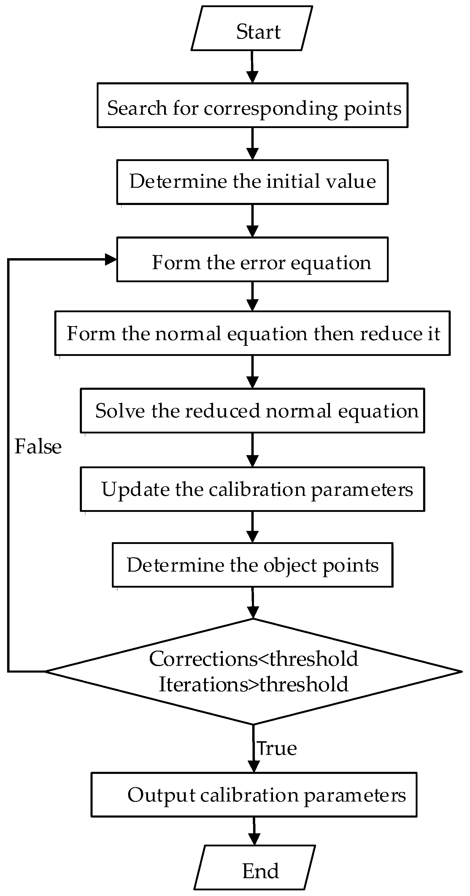
2.3. Processing Procedure
Figure 2 shows the processing procedure of the proposed method. The detailed procedure is as follows:
- (1)
- (2)
- Determine the initial value of the unknown parameters. Initial calibration parameters can be assigned to laboratory calibration values acquired from the calibration work in the laboratory before the satellite launch. Although laboratory calibration values have changed during the launch process due to factors such as the release of stress, it can be still set as the initial value of calibration parameters. On this basis, the correction of calibration parameters can be assigned to zero. And the unknown object coordinates can be determined by forward intersection between the corresponding points of the images.
- (3)
- Form the error equation point by point. The linearized calibration equation can be constructed according to Equation (6). The process should be applied to every point to form the error equation as in Equation (9).
- (4)
- Form the normal equation, then reduce it. The normal equation can be formed according to Equation (11), and the reduced normal equation for the correction to calibration parameters from the normal equation is Equation (12).
- (5)
- Use the ICCV method to solve the reduced normal equation, and thereby acquire the correction to the calibration parameters.
- (6)
- Update calibration parameters by adding the corrections.
- (7)
- Determine the coordinates of object points by forward intersection.
- (8)
- Execute steps (3)–(7) iteratively until calibration parameters tend to be convergent and stable. Otherwise, the procedure provides the updated calibration parameters and terminates. Here the iterations and corrections can be set an empirical threshold respectively to terminate the iteration.
3. Results and Discussion
The accuracy and reliability of the proposed method were verified by experiments using images captured by the GF-1 WFV-1 camera. Launched in April 2013, the GF-1 satellite is installed with a set of four WFV cameras with 16 m multispectral resolution and a total swath of 800 km [33,34,35]. Detailed information about the GF-1 WFV cameras is given in Table 2. To validate the proposed method, positioning accuracies before and after applying calibration parameters to images from GF-1 WFV-1 were assessed by check points (CPs) that were obtained from GCF images by high-precision matching methods [3,6,7] or were manually extracted from Google Earth. To validate the effect of interior calibration parameters for compensating camera interior distortions, the affine model for images was adopted as the exterior orientation model to remove other errors caused by exterior elements [36,37] for the reason that images acquired in different times possess different exterior calibration parameters, and the orientation accuracies between and after correction were validated. Moreover, the proposed method and classic GCF were compared.
3.1. Datasets
Several GF-1 WFV-1 images were collected in order to sufficiently detect and eliminate distortion. Table 3 details the experimental images, which cover Shanxi and Henan provinces in China. The experiment below assesses the orientation accuracy before and after applying the calibration parameters acquired from the proposed method. The residual error of CPs reflects the compensation for interior distortion in each WFV-1 image.
Scenes 068316, 108244, and 125565 were used to detect distortions by the proposed method (Table 3). Then, scenes 068316, 108244, 125565, and 126740 were used to validate orientation accuracy according to the GCPs acquired from the GCF. Finally, scenes 068316, 079476, 125567, and 132279 were used to validate orientation accuracy according to the CPs acquired from Google Earth. To compare the proposed method with the classical method, we also have compensated for distortion by calibration parameters obtained by the classical method, and validated the orientation of scenes 068316, 079476, 125567, and 132279 according to CPs acquired from Google Earth.
3.2. Distortion Detection
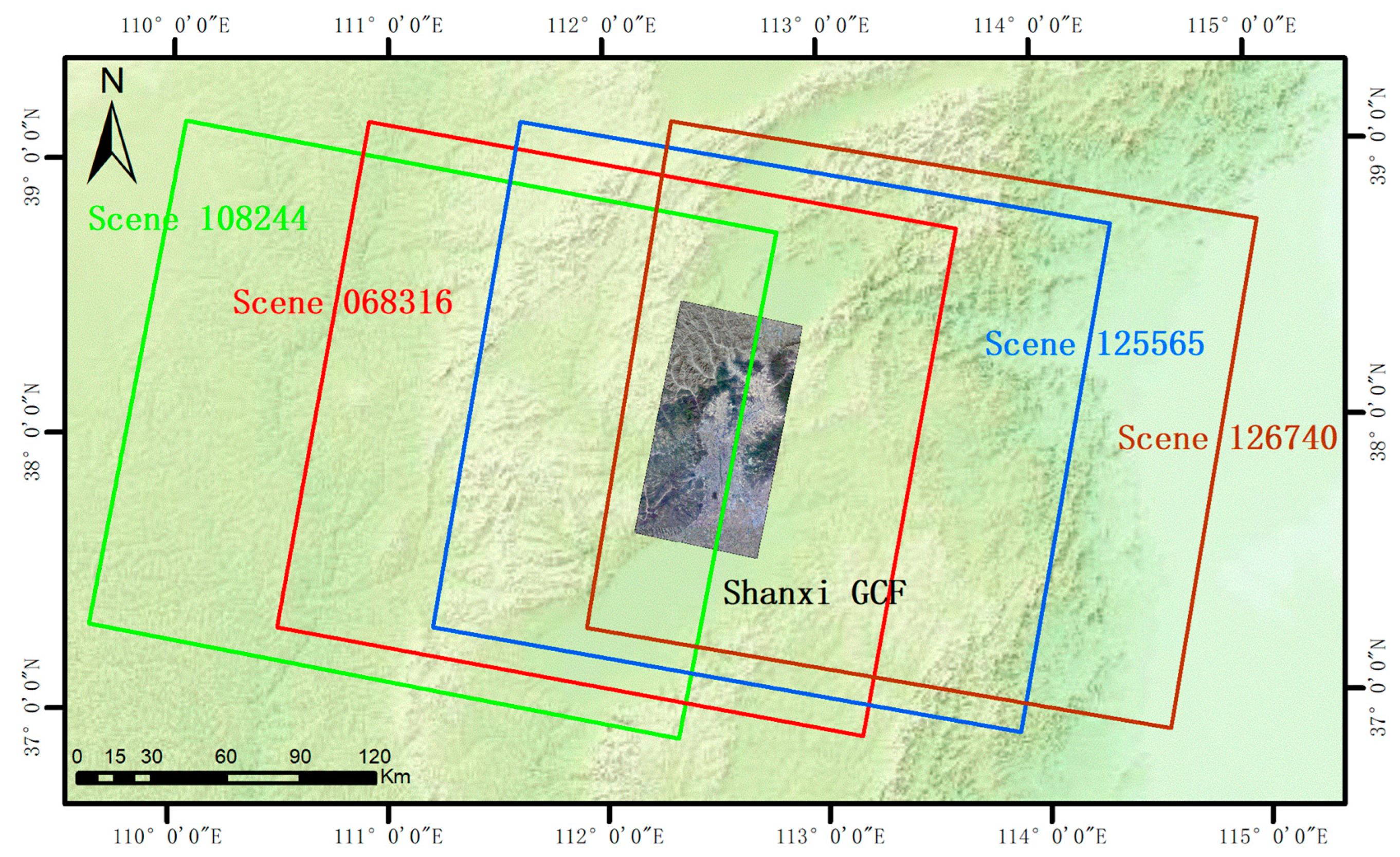
Calibration parameters were acquired from images of the Shanxi area (scenes 068316, 108244, and 125565) by the proposed method. The range of scenes are shown in Figure 3. The three scenes overlap each other in the mountainous area. In order to apply the proposed method to detect distortion, 19,193 evenly distributed corresponding points between these images were obtained from the overlap area, as shown in Figure 4. After obtaining sufficient corresponding points, the calibration parameters were acquired using the proposed method.
To verify whether the calibration parameters could work, they were applied to scenes 108244, 068316, 125565, and 126740 to verify the orientation accuracy. CPs were acquired by the method introduced in Huang et al. [6] using the Shanxi GCF, which includes a 1:5000 digital DOM and DEM (Table 1). The sample range represents coverage of the GCF for the start and end rows of images across the track (Figure 3). The orientation accuracy is presented in Table 4.
The accuracy level after orientation is less than 1 pixel for both the original and compensated scenes, and the distortion error is mainly reflected across the track. The orientation accuracy of the compensated scene is improved if compared to the original scene, especially for scenes 108244 and 126740. Moreover, GCPs of the two scenes are at the ends of the sample, illustrating that distortion is more severe at the ends.
The exterior orientation absorbed some interior errors, because the sample range only covers a part of the image. Therefore, it is difficult to observe any residual distortion from Table 4. To observe residual distortion, residual errors before and after compensation are respectively shown in Figure 5a,b.
Although the original scenes have an orientation accuracy as high as 1 pixel for residual errors before compensation, they exhibit a systematic pattern, as shown in Figure 5a, especially at both ends. Distortions that seriously affect application of the satellite images should be detected and corrected.
As shown in Figure 5b, after compensating for the distortions, residual errors are random and are constrained within 0.6 pixel, meaning that all distortions have been corrected and the calibration parameters acquired by the proposed method are effective.
3.3. Accuracy Validation
After calculating the calibration parameters by the proposed method, it is important to verify whether the calibration parameters can be used in other scenes.
As the GCF has a range restriction and the swath width of the GF1 WFV camera reaches 200 km, CPs from the GCF can only cover some rows of each image. Thus, the exterior orientation will absorb some interior errors, thereby influencing the orientation accuracy of the whole image. Many studies have shown that the horizontal positioning accuracy of Google Earth is better than 3 m [38,39,40]. Given that the resolution of GF-1 WFV is 16 m, the accuracy of Google Earth renders it appropriate for validation and to illustrate the influence of compensation.
The conventional GCF method according to Huang et al. [6] was applied to acquire calibration parameters compensating for distortion, thus permitting a comparison between the proposed method and the classic GCF method.
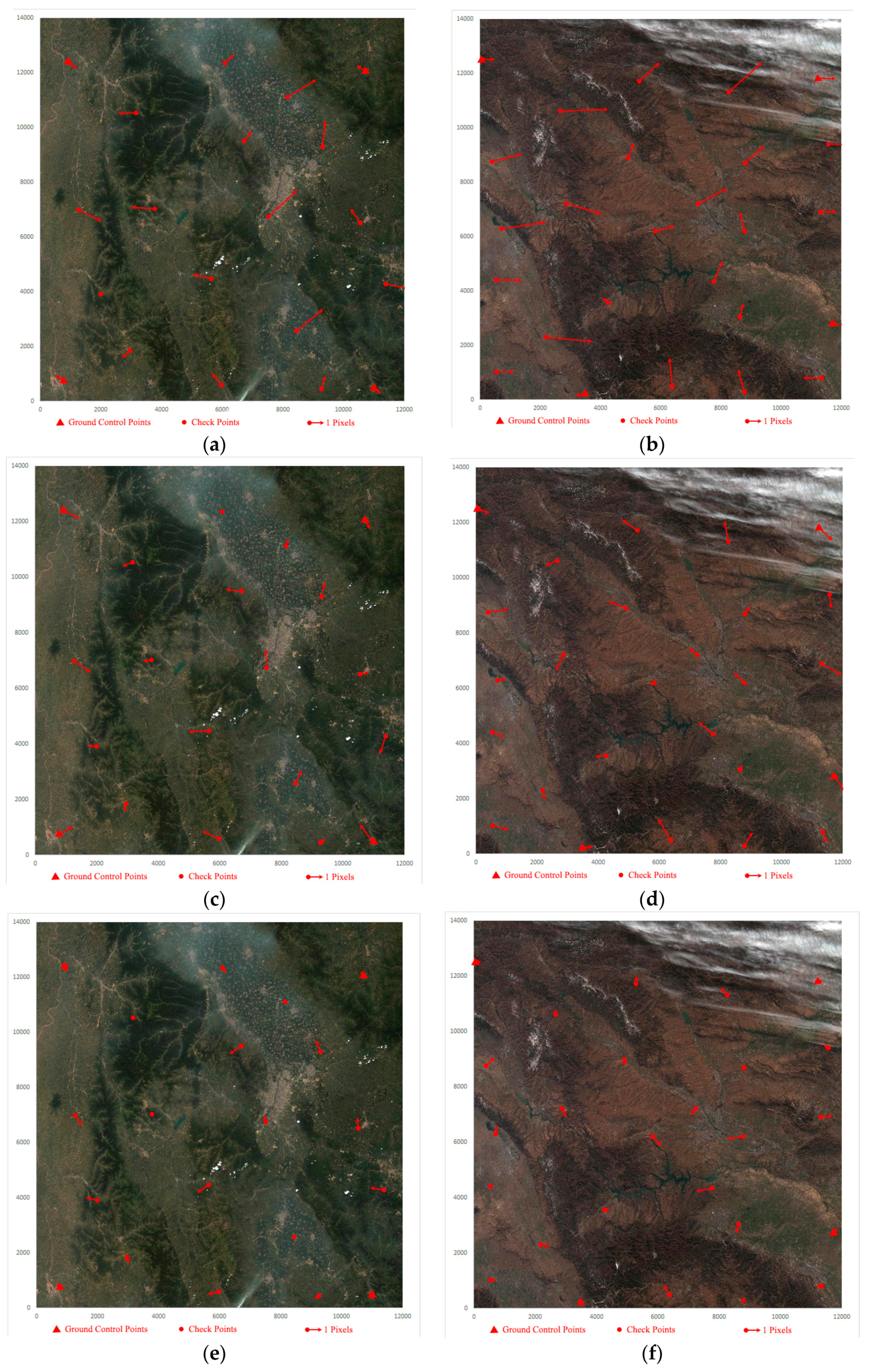
The results are shown in Table 5. To observe the residual, the orientation errors of scenes 068316 and 125567 with four GCPs are shown in Figure 6.
As shown in Table 5, the maximum orientation errors without calibration parameters are about 5.5 pixels and the orientation accuracy is only 2 pixels. These errors result partly from the distortion implied in the original scenes. Thus, when the original scenes are compensated by calibration parameters acquired by the proposed method, the maximum orientation errors are reduced to less than 2.6 pixels; in particular, the errors in scene 068316 are reduced to around 1.5 pixels.
The orientation errors of scenes 068316 and 125567 without calibration parameters are shown in Figure 6a,b, respectively, and following treatment by the proposed method are shown in Figure 6c,d respectively. The level of orientation accuracy of the compensated scenes obtained by the proposed method is consistently around 1 pixel, illustrating that the proposed method can provide effective compensation for distortions.
However, from Table 5 we can also observe that the orientation accuracy of the proposed method is lower than that of the classical method, whether in line or sample. This can be seen in Figure 6c,e of scene 068316, or Figure 6d,f of scene 125567.
There are several reasons that may explain the lower accuracy of the proposed method. The first is lack of absolute reference. Unlike the classical method, the proposed method is conducted without the aid of absolute references:this is the key reason for the low accuracy obtained. Secondly, strong correlation between calibration parameters results from the lack of absolute reference in the proposed method. Although the ICCV method can partially resolve this problem, it will also influence the result. Thirdly, over-parameterization of the calibration model may be a factor. In the calibration model (Equation (3)), the highest order term of the polynomial is 5. However, Figure 5a shows that the highest order term may not reach 5, especially in the line direction. Over-parameterization of the calibration model will result in over-fitting, especially without absolute references, as in the proposed method. Finally, the quality of the corresponding points may reduce accuracy. The proposed method requires corresponding points from at least three overlapping images, so the registration accuracy, distribution, and number of corresponding points will also influence the results.
4. Conclusions
In this study, a novel method was proposed to correct interior distortions of pushbroom satellite imagery independent of ground control points (GCPs). The proposed method uses at least three overlapping images, and takes advantage of the forward intersection residual between corresponding points in the images to calculate interior distortions. Images captured by Gaofen-1 (GF-1) wide field view-1 (WFV-1) camera were collected as experimental data. Several conclusions can be drawn as follows:
- The proposed method can compensate for interior distortions and effectively improve the internal accuracy for pushbroom satellite imagery. After applying the calibration parameters acquired by the proposed method, images orientation accuracies evaluated by Ground Control Field (GCF) are within 0.6 pixel, with residual errors manifesting as random errors. Validation using Google Earth CPs further validates that the proposed method can improve orientation accuracy to within 1 pixel, and the entire scene is undistorted compared with that without calibration parameters compensating.
- In this paper, with the proposed method affected by unfavorable factors, such as lack of absolute references, over-parameterization of the calibration model and original image quality, the result is slightly inferior to the traditional GCF method and there exists maximum difference being approximately 0.4 pixel finally.
We can conclude that the proposed method can correct the interior distortions and improve the internal geometric quality for satellite imagery when there is no appropriate GCF to perform the classic method. Despite the promising results achieved for GF-1 WFV-1 camera, only one of the four WFV cameras onboard the satellite is considered. For the correction of four WFV cameras onboard GF-1 independent of GCPs simultaneously, further researche is required.
Acknowledgments
This work was supported by, Key research and development program of Ministry of science and technology (2016YFB0500801), National Natural Science Foundation of China (Grant No. 91538106, Grant No. 41501503, 41601490, Grant No. 41501383), China Postdoctoral Science Foundation (Grant No. 2015M582276), Hubei Provincial Natural Science Foundation of China (Grant No. 2015CFB330), Special Fund for High Resolution Images Surveying and Mapping Application System (Grant No. AH1601-10), Quality improvement of domestic satellite data and comprehensive demonstration of geological and mineral resources (Grant No. DD20160067). The authors also thank the anonymous reviews for their constructive comments and suggestions.
Author Contributions
Kai Xu, Guo Zhang and Deren Li conceived and designed the experiments; Kai Xu, Guo Zhang, and Qingjun Zhang performed the experiments; Kai Xu, Guo Zhang and Deren Li analyzed the data; Kai Xu wrote the paper.
Conflicts of Interest
The authors declare no conflict of interest.
References
- Baltsavias, E.; Zhang, L.; Eisenbeiss, H. Dsm generation and interior orientation determination of IKONOS images using a testfield in Switzerland. Photogramm. Fernerkund. Geoinf. 2006, 1, 41–54. [Google Scholar]
- Zhang, L.; Gruen, A. Multi-image matching for DSM generation from IKONOS imagery. ISPRS J. Photogramm. Remote Sens. 2006, 60, 195–211. [Google Scholar] [CrossRef]
- Leprince, S.; Musé, P.; Avouac, J.P. In-flight CCD distortion calibration for pushbroom satellites based on subpixel correlation. IEEE Trans. Geosci. Remote Sens. 2008, 46, 2675–2683. [Google Scholar] [CrossRef]
- CNES (Centre National d’Etudes Spatiales). Spot Image Quality Performances. Available online: http://www.spot.ucsb.edu/spot-performance.pdf (acessed on 15 May 2004).
- Greslou, D.; Delussy, F.; Delvit, J.; Dechoz, C.; Amberg, V. PLEIADES-HR Innovative Techniquesfor Geometric Image Quality Commissioning. In Proceedings of the 2012 XXII ISPRS CongressInternational Archives of the Photogrammetry, Remote Sensing and Spatial Information Sciences, Melbourne, VIC, Australia, 25 August–1 September 2012; pp. 543–547. [Google Scholar]
- Huang, W.C.; Zhang, G.; Tang, X.M.; Li, D.R. Compensation for distortion of basic satellite images based on rational function model. IEEE J. Sel. Top. Appl. Earth Obs. Remote Sens. 2016, 9, 5767–5775. [Google Scholar] [CrossRef]
- Leprince, S.; Barbot, S.; Ayoub, F.; Avouac, J.P. Automatic and precise orthorectification, coregistration, and subpixel correlation of satellite images, application to ground deformation measurements. IEEE Trans. Geosci. Remote Sens. 2007, 45, 1529–1558. [Google Scholar] [CrossRef]
- Zhang, G.; Jiang, Y.H.; Li, D.R.; Huang, W.C.; Pan, H.B.; Tang, X.M.; Zhu, X.Y. In-orbit geometric calibration and validation of ZY-3 linear array sensors. Photogramm. Rec. 2014, 29, 68–88. [Google Scholar] [CrossRef]
- Jiang, Y.H.; Zhang, G.; Tang, X.M.; Li, D.R.; Huang, W.C.; Pan, H.B. Geometric calibration and accuracy assessment of ZiYuan-3 multispectral images. IEEE Trans. Geosci. Remote Sens. 2014, 52, 4161–4172. [Google Scholar] [CrossRef]
- Fraser, C.S. Digital camera self-calibration. ISPRS J. Photogramm. Remote Sens. 1997, 52, 149–159. [Google Scholar] [CrossRef]
- Habib, A.F.; Michel, M.; Young, R.L. Bundle adjustment with self–calibration using straight lines. Photogramm. Rec. 2010, 17, 635–650. [Google Scholar] [CrossRef]
- Sultan, K.; Armin, G. Orientation and self-calibration of ALOS PRISM imagery. Photogramm. Rec. 2008, 23, 323–340. [Google Scholar] [CrossRef]
- Gonzalez, S.; Gomez-Lahoz, J.; Gonzalez-Aguilera, D.; Arias, B.; Sanchez, N.; Hernandez, D.; Felipe, B. Geometric analysis and self-calibration of ADS40 imagery. Photogramm. Rec. 2013, 28, 145–161. [Google Scholar] [CrossRef]
- Di, K.C.; Liu, Y.L.; Liu, B.; Peng, M.; Hu, W.M. A self-calibration bundle adjustment method for photogrammetric processing of Chang’e-2 stereo lunar imagery. IEEE Trans. Geosci. Remote Sens. 2014, 52, 5432–5442. [Google Scholar] [CrossRef]
- Zheng, M.T.; Zhang, Y.J.; Zhu, J.F.; Xiong, X.D. Self-calibration adjustment of CBERS-02B long-strip imagery. IEEE Trans. Geosci. Remote Sens. 2015, 53, 3847–3854. [Google Scholar] [CrossRef]
- Kubik, P.; Lebègue, L.; Fourest, F.; Delvit, J.M.; Lussy, F.D.; Greslou, D.; Blanchet, G. First in-flight results of PLEIADES 1A innovative methods for optical calibration. In Proceedings of the International Conference on Space Optics—ICSO 2012, Ajaccio, France, 9–12 October 2012. [Google Scholar] [CrossRef]
- Dechoz, C.; Lebègue, L. PLEIADES-HR 1A&1B image quality commissioning: Innovative geometric calibration methods and results. In Proceedings of the SPIE—The International Society for Optical Engineering, San Diego, CA, USA, 23 September 2013; Volume 8866, p. 11. [Google Scholar] [CrossRef]
- De Lussy, F.; Greslou, D.; Dechoz, C.; Amberg, V.; Delvit, J.M.; Lebegue, L.; Blanchet, G.; Fourest, S. PLEIADES-HR in flight geometrical calibration: Location and mapping of the focal plane. In Proceedings of the 2012 XXII ISPRS CongressInternational Archives of the Photogrammetry, Remote Sensing and Spatial Information Sciences, Melbourne, VIC, Australia, 25 August–1 September 2012; pp. 519–523. [Google Scholar]
- Delevit, J.M.; Greslou, D.; Amberg, V.; Dechoz, C.; De Lussy, F.; Lebegue, L.; Latry, C.; Artigues, S.; Bernard, L. Attitude assessment using PLEIADES-HR capabilities. In Proceedings of the 2012 XXII ISPRS CongressInternational Archives of the Photogrammetry, Remote Sensing and Spatial Information Sciences, Melbourne, VIC, Australia, 25 August–1 September 2012; pp. 525–530. [Google Scholar]
- Faugeras, O.D.; Luong, Q.T.; Maybank, S.J. Camera Self-Calibration: Theory and Experiments. In Proceedings of the European Conference on Computer Vision; Springer: Berlin/Heidelberg, Germany, 1992; pp. 321–334. [Google Scholar]
- Hartley, R.I. Self-calibration of stationary cameras. Int. J. Comput. Vis. 1997, 22, 5–23. [Google Scholar] [CrossRef]
- Malis, E.; Cipolla, R. Self-calibration of zooming cameras observing an unknown planar structure. In Proceedings of the 15th International Conference on Pattern Recognition, Barcelona, Spain, 3–8 September 2000; pp. 85–88. [Google Scholar]
- Malis, E.; Cipolla, R. Camera self-calibration from unknown planar structures enforcing the multiview constraints between collineations. IEEE Trans. Pattern Anal. Mach. Intell. 2002, 24, 1268–1272. [Google Scholar] [CrossRef]
- Tang, X.M.; Zhu, X.Y.; Pan, H.B.; Jiang, Y.H.; Zhou, P.; Wang, X. Triple linear-array image geometry model of ZiYuan-3 surveying satellite and its validation. Acta Geod. Cartogr. Sin. 2012, 4, 33–51. [Google Scholar] [CrossRef]
- Xu, K.; Jiang, Y.H.; Zhang, G.; Zhang, Q.J.; Wang, X. Geometric potential assessment for ZY3–02 triple linear array imagery. Remote Sens. 2017, 9, 658. [Google Scholar] [CrossRef]
- Xu, J.Y. Study of CBERS CCD camera bias matix calculation and its application. Spacecr. Recover. Remote Sens. 2004, 4, 25–29. [Google Scholar]
- Yuan, X.X. Calibration of angular systematic errors for high resolution satellite imagery. Acta Geod. Cartogr. Sin. 2012, 41, 385–392. [Google Scholar]
- Radhadevi, P.V.; Solanki, S.S. In-flight geometric calibration of different cameras of IRS-P6 using a physical sensor model. Photogramm. Rec. 2010, 23, 69–89. [Google Scholar] [CrossRef]
- Bouillon, A. Spot5 HRG and HRS first in-flight geometric quality results. Int. Symp. Remote Sens. 2003, 4881, 212–223. [Google Scholar] [CrossRef]
- Bouillon, A.; Breton, E.; Lussy, F.D.; Gachet, R. Spot5 geometric image quality. In Proceedings of the IEEE International Geoscience and Remote Sensing Symposium, Toulouse, France, 21–25 July 2003; pp. 303–305. [Google Scholar]
- Mulawa, D. On-orbit geometric calibration of the Orbview-3 high resolution imaging satellite. Int. Arch. Photogramm. Remote Sens. Spat. Inf. Sci 2004, 35, 1–6. [Google Scholar]
- Wang, X.Z.; Liu, D.Y.; Zhang, Q.Y.; Huang, H.L. The iteration by correcting characteristic value and its application in surveying data processing. J. Heilongjiang Inst. Technol. 2001, 15, 3–6. [Google Scholar] [CrossRef]
- Bai, Z.G. Gf-1 satellite-the first satellite of CHEOS. Aerosp. China 2013, 14, 11–16. [Google Scholar]
- Lu, C.L.; Wang, R.; Yin, H. Gf-1 satellite remote sensing characters. Spacecr. Recover. Remote Sens. 2014, 35, 67–73. [Google Scholar]
- XinHuaNet. China Launches Gaofen-1 Satellite. Available online: http://news.xinhuanet.com/photo/2013–04/26/c_124636364.htm (accessed on 26 April 2013).
- Fraser, C.S.; Hanley, H.B. Bias compensation in rational functions for IKONOS satellite imagery. Photogramm. Eng. Remote Sens. 2015, 69, 53–58. [Google Scholar] [CrossRef]
- Fraser, C.S.; Yamakawa, T. Insights into the affine model for high-resolution satellite sensor orientation. ISPRS J. Photogramm. Remote Sens. 2004, 58, 275–288. [Google Scholar] [CrossRef]
- Wirth, J.; Bonugli, E.; Freund, M. Assessment of the accuracy of Google Earth imagery for use as a tool in accident reconstruction. SAE Tech. Pap. 2015, 1, 1435. [Google Scholar] [CrossRef]
- Pulighe, G.; Baiocchi, V.; Lupia, F. Horizontal accuracy assessment of very high resolution Google Earth images in the city of Rome, Italy. Int. J. Digit. Earth 2015, 9, 342–362. [Google Scholar] [CrossRef]
- Farah, A.; Algarni, D. Positional accuracy assessment of GoogleEarth in Riyadh. Artif. Satell. 2014, 49, 101–106. [Google Scholar] [CrossRef]
Figure 1.
Schematic diagram showing correction of distortion independent of (GCPs). (a) Two images are insufficient to detect image distortion; (b) three images can detect image distortion.
Figure 1.
Schematic diagram showing correction of distortion independent of (GCPs). (a) Two images are insufficient to detect image distortion; (b) three images can detect image distortion.

Figure 2.
Proposed processing procedure of distortion detection without using ground control points (GCPs).
Figure 2.
Proposed processing procedure of distortion detection without using ground control points (GCPs).

Figure 3.
Coverage of images 108244, 068316, 125565, and 126740 and the GCF in Shanxi.

Figure 4.
Corresponding points for distortion detection scenes selected from (a) scene 108244; (b) scene 068316; and (c) scene 125565.
Figure 4.
Corresponding points for distortion detection scenes selected from (a) scene 108244; (b) scene 068316; and (c) scene 125565.
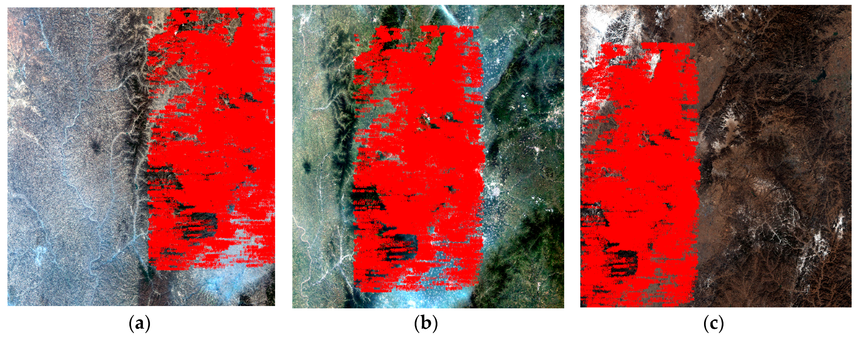
Figure 5.
Residual errors (a) before; and (b) after compensation for distortion (horizontal axis denotes the image row across the track and vertical axis denotes residual errors after orientation).
Figure 5.
Residual errors (a) before; and (b) after compensation for distortion (horizontal axis denotes the image row across the track and vertical axis denotes residual errors after orientation).
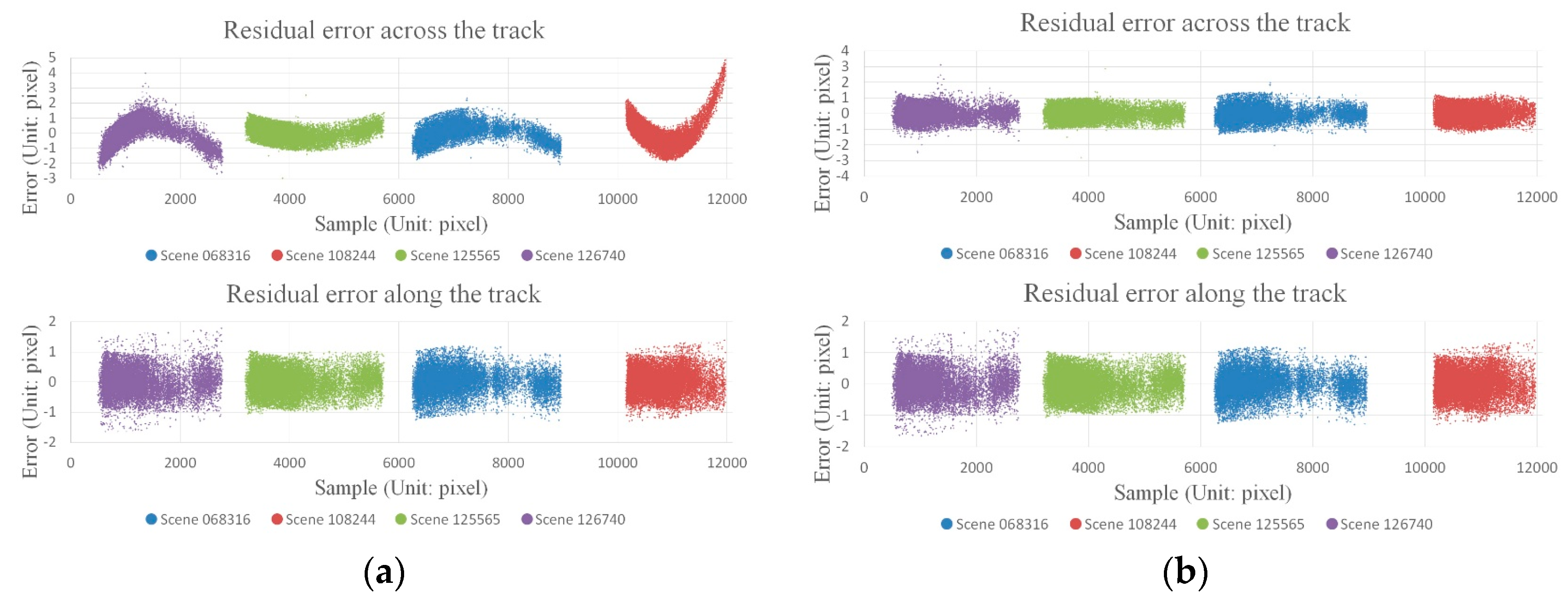
Figure 6.
Orientation errors with four GCPs in (a) scene 068316; and (b) scene 125567, before correcting distortion; (c) scene 068316; and (d) scene 125567, after applying the proposed method; and (e) scene 068316; and (f) scene 125567, after applying the classic GCF method.
Figure 6.
Orientation errors with four GCPs in (a) scene 068316; and (b) scene 125567, before correcting distortion; (c) scene 068316; and (d) scene 125567, after applying the proposed method; and (e) scene 068316; and (f) scene 125567, after applying the classic GCF method.


Table 1.
Currently available GCFs in China.
| Area | GSD of DOM (m) | Plane Accuracy of DOM RMS (m) | Height Accuracy of DEM RMS (m) | Range (km2) (Across Track × Along Track) | Center (Latitude and Longitude) |
|---|---|---|---|---|---|
| Shanxi | 0.5 | 1 | 1.5 | 50 × 95 | 38.00°N, 112.52°E |
| Songshan | 0.5 | 1 | 1.5 | 50 × 41 | 34.65°N, 113.55°E |
| Dengfeng | 0.2 | 0.4 | 0.7 | 54 × 84 | 34.45°N, 113.07°E |
| Tianjin | 0.2 | 0.4 | 0.7 | 72 × 54 | 39.17°N, 117.35°E |
| Northeast | 0.5 | 1 | 1.5 | 100 × 600 | 45.50°N, 125.63°E |
Table 2.
Characteristics of the WFV camera onboard GF-1.
| Items | Values |
|---|---|
| Swath | 200 km |
| Resolution | 16 m |
| Change-coupled device (CCD) size | 0.0065 mm |
| Principle distance | 270 mm |
| Field of view (FOV) | 16.44 degrees |
| Image size | 12,000 × 13,400 pixels |
Table 3.
GF-1 WFV-1 images used in method validation.
| Scene ID | Area | Image Date | No. of CPs | Sample Range (Pixel) | Function |
|---|---|---|---|---|---|
| 068316 | Shanxi | 10 August 2013 | 15,800 | 6300–9000 | Detection/Validation |
| 108244 | Shanxi | 7 November 2013 | 18,057 | 10,200–12,000 | Detection/Validation |
| 125565 | Shanxi | 27 November 2013 | 19,459 | 3200–5700 | Detection/Validation |
| 126740 | Shanxi | 5 December 2013 | 14,551 | 500–2700 | Validation |
| 079476 | Henan | 3 September 2013 | —— | —— | Validation |
| 125567 | Henan | 27 November 2013 | —— | —— | Validation |
| 132279 | Henan | 13 December 2013 | —— | —— | Validation |
Table 4.
Orientation accuracy before and after compensation for distortion (unit: pixel).
| Scene ID | No. GCPs/CPs | Sample Range (Pixel) | Line (along the Track) | Sample (across the Track) | Max | Min | RMS | |
|---|---|---|---|---|---|---|---|---|
| 068316 | 4/15,796 | 6300–9000 | Ori. 1 | 0.383 | 0.537 | 2.345 | 0.005 | 0.660 |
| Com. 2 | 0.384 | 0.416 | 2.022 | 0.005 | 0.566 | |||
| 108244 | 4/18,053 | 10,200–12,000 | Ori. | 0.382 | 0.864 | 4.863 | 0.005 | 0.945 |
| Com. | 0.382 | 0.412 | 1.656 | 0.004 | 0.562 | |||
| 125565 | 4/19,455 | 3200–5700 | Ori. | 0.374 | 0.428 | 3.045 | 0.005 | 0.569 |
| Com. | 0.374 | 0.375 | 3.015 | 0.007 | 0.530 | |||
| 126740 | 4/14,547 | 500–2700 | Ori. | 0.432 | 0.813 | 3.973 | 0.009 | 0.920 |
| Com. | 0.432 | 0.439 | 3.117 | 0.008 | 0.616 |
1 Ori indicates accuracy after orientation without calibration parameters; 2 Com represents accuracy after orientation with the calibration parameters obtained by the proposed method.
Table 5.
Orientation accuracy with four ground control points (GCPs) (unit: pixel).
| Scene ID | No. GCPs/CPs | Line (along the Track) | Sample (across the Track) | Max | Min | RMS | |
|---|---|---|---|---|---|---|---|
| 068316 | 4/16 | Ori. 1 | 0.916 | 1.069 | 2.692 | 0.207 | 1.410 |
| Pro. 2 | 0.701 | 0.701 | 1.529 | 0.215 | 0.991 | ||
| Cla. 3 | 0.430 | 0.437 | 0.991 | 0.130 | 0.613 | ||
| 079476 | 4/24 | Ori. | 0.840 | 1.921 | 5.538 | 0.512 | 2.097 |
| Pro. | 0.846 | 0.780 | 2.543 | 0.119 | 1.164 | ||
| Cla. | 0.646 | 0.635 | 1.788 | 0.088 | 0.906 | ||
| 125567 | 4/22 | Ori. | 0.966 | 1.721 | 3.173 | 0.541 | 1.973 |
| Pro. | 0.760 | 0.748 | 1.803 | 0.305 | 1.067 | ||
| Cla. | 0.384 | 0.433 | 1.072 | 0.079 | 0.579 | ||
| 132279 | 4/22 | Ori. | 0.790 | 1.991 | 4.922 | 0.249 | 2.142 |
| Pro. | 0.798 | 0.779 | 2.050 | 0.145 | 1.115 | ||
| Cla. | 0.525 | 0.505 | 1.198 | 0.054 | 0.728 |
1 Ori indicates accuracy after orientation without calibration parameters; 2 Pro denotes accuracy after orientation with calibration parameters acquired from the proposed method; 3 Cla represents accuracy after orientation with calibration parameters obtained from the classic method.
© 2018 by the authors. Licensee MDPI, Basel, Switzerland. This article is an open access article distributed under the terms and conditions of the Creative Commons Attribution (CC BY) license (http://creativecommons.org/licenses/by/4.0/).
Share and Cite
MDPI and ACS Style
Zhang, G.; Xu, K.; Zhang, Q.; Li, D. Correction of Pushbroom Satellite Imagery Interior Distortions Independent of Ground Control Points. Remote Sens. 2018, 10, 98. https://doi.org/10.3390/rs10010098
AMA Style
Zhang G, Xu K, Zhang Q, Li D. Correction of Pushbroom Satellite Imagery Interior Distortions Independent of Ground Control Points. Remote Sensing. 2018; 10(1):98. https://doi.org/10.3390/rs10010098
Chicago/Turabian StyleZhang, Guo, Kai Xu, Qingjun Zhang, and Deren Li. 2018. "Correction of Pushbroom Satellite Imagery Interior Distortions Independent of Ground Control Points" Remote Sensing 10, no. 1: 98. https://doi.org/10.3390/rs10010098
Note that from the first issue of 2016, this journal uses article numbers instead of page numbers. See further details here.