A Novel Index for Impervious Surface Area Mapping: Development and Validation


College of Information Engineering, China University of Geosciences, Wuhan 430074, China
*
Author to whom correspondence should be addressed.
Remote Sens. 2018, 10(10), 1521; https://doi.org/10.3390/rs10101521
Submission received: 31 August 2018
/
Revised: 14 September 2018
/
Accepted: 20 September 2018
/
Published: 22 September 2018
Abstract
:The distribution and dynamic changes in impervious surface areas (ISAs) are crucial to understanding urbanization and its impact on urban heat islands, earth surface energy balance, hydrological cycles, and biodiversity. Remotely sensed data play an essential role in ISA mapping, and numerous methods have been developed and successfully applied for ISA extraction. However, the heterogeneity of ISA spectra and the high similarity of the spectra between ISA and soil have not been effectively addressed. In this study, we selected data from the US Geological Survey (USGS) and Advanced Spaceborne Thermal Emission and Reflection Radiometer (ASTER) spectral libraries as samples and used blue and near-infrared bands as characteristic bands based on spectral analysis to propose a novel index, the perpendicular impervious surface index (PISI). Landsat 8 operational land imager data in four provincial capital cities of China (Wuhan, Shenyang, Guangzhou, and Xining) were selected as test data to examine the performance of the proposed PISI in four different environments. Threshold analysis results show that there is a significant positive correlation between PISI and the proportion of ISA, and threshold can be adjusted according to different needs with different accuracy. Furthermore, comparative analyses, which involved separability analysis and extraction precision analysis, were conducted among PISI, biophysical composition index (BCI), and normalized difference built-up index (NDBI). Results indicate that PISI is more accurate and has better separability for ISA and soil as well as ISA and vegetation in the ISA extraction than the BCI and NDBI under different conditions. The accuracy of PISI in the four cities is 94.13%, 96.50%, 89.51%, and 93.46% respectively, while BCI and NDBI showed accuracy of 77.53%, 93.49%, 78.02%, and 84.03% and 58.25%, 57.53%, 77.77%, and 64.83%, respectively. In general, the proposed PISI is a convenient index to extract ISA with higher accuracy and better separability for ISA and soil as well as ISA and vegetation. Meanwhile, as PISI only uses blue and near-infrared bands, it can be used in a wider variety of remote sensing images.
1. Introduction
Impervious surface areas (ISAs) have been experiencing dramatic expansion accompanied by rapid urbanization worldwide [1]. ISA expansion significantly alters land surface characteristics in a transformation from a natural landscape to an anthropogenic landscape, which presents serious problems for urban environmental quality, such as aggravating the urban heat island effect [2,3,4,5,6,7], enhancing the speed and volume of urban runoff, with increased pressure for municipal drainage and flood control [8], and reducing groundwater recharge [9]. Consequently, timely and accurate monitoring of ISA dynamics is becoming urgent for the strategic planning of urban development and the projection of ISA environmental impacts [10].
Remote sensing has been widely used for ISA mapping and dynamics monitoring at multiple spatial resolutions with different satellite data [11,12,13,14]. Generally, the methods for ISA mapping can be grouped into three major categories: classification-based, mixture analysis, and index-based methods. For the classification-based methods, supervised classifiers that are supported by numerous training samples are used, including maximum likelihood classifier [15], support vector machine [16], artificial neural networks [17], random forest [18], and object-oriented methods [19]. However, the classification-based method has produced unsatisfactory results in many applications, given the spectral and textural complexity of ISA and the extensive existence of mixed pixels with various combinations of ISA and other land cover types [20].
The mixture analysis methods can be classified into two subcategories, spectral mixture analysis (SMA) [21,22,23] and temporal mixture analysis (TMA) [24,25,26]. Spectral mixture analysis assumes that, in a given geographical scene, the surface is composed of several features (i.e., endmembers) and the spectral characteristics of these features are relatively stable. Therefore, the reflectance of the pixels in remote sensing images can be represented as a function of the spectral characteristics of features and the endmember proportion (abundance). Generally, SMA follows the vegetation–ISA–soil (VIS) model [27] to derive ISA fractions, in which ISA, vegetation, and soil are treated as typical endmembers. TMA, another mixture method, also follows the VIS model. It differs from SMA in that TMA uses the temporal spectra of land cover types rather than the electromagnetic spectra. The results of the mixture analysis methods heavily depend on endmember selection, which remains a challenge, because the differences in materials used, geometry, and illumination produce obvious spectral variability of ISA [28,29]. The within-class variability and collinearity of endmembers may generate large errors [24,30,31].
In comparison with those two methods, the index-based methods are easy to implement in practical applications with minimal effort in selecting training samples and endmembers. The typical indices specified for ISA mapping, including normalized difference built-up index (NDBI) [32], normalized difference impervious surface index (NDISI) [33], modified NDISI (MNDISI) [34], and biophysical composition index (BCI) [35], are widely used. In detail, the NDBI uses shortwave-infrared (SWIR) and near-infrared (NIR) bands to distinguish ISAs. The performance is less satisfactory in areas with large amounts of soil, because NDBI can easily confuse ISAs with soil [36]. The NDISI uses visible, NIR, mid-infrared, and thermal-infrared bands to develop the index, thereby assuming that the ISA material has relatively stable spectral characteristics despite the effects of aging, degradation, and paints on the ISA spectra. The NDISI highly depends on land-surface temperature data, resulting in failures in areas with a weak heat island effect. The MNDISI introduces nighttime light luminosity and a soil-adjusted vegetation index to enhance the ISA characteristics; however, the MNDISI is inconvenient to apply and is restricted by data sources. The BCI performs the tasseled cap (TC) transformation in advance and uses the first three TC components to extract ISA. However, a few sensors do not have the corresponding TC transformation matrix.
Index-based methods, which are widely used, are characterized by simplicity and flexibility. Nevertheless, problems remain to be addressed. First, ISA and soil are easily confused [28,37,38]. Second, certain indices require various data sources or complex operations; however, a few sensors do not cover the bands of SWIR, mid-infrared, and thermal infrared and lack the corresponding TC transformation matrix. Thus, indices such as the BCI cannot be used in several cases. Third, most of the aforementioned indices are poorly qualified for certain remotely sensed images, which commonly consist of four bands: blue, green, red, and NIR. In this paper, based on the analysis of samples selected from US Geological Survey (USGS) and Advanced Spaceborne Thermal Emission and Reflection Radiometer (ASTER) spectral libraries, we propose a novel index using blue and near-infrared bands, the perpendicular impervious surface index (PISI). Our goals are: (1) to eliminate or reduce soil and vegetation interference to ensure that the PISI has high accuracy for ISA extraction at medium-resolution remotely sensed images in different scenes; and (2) to explore the ability of our index to be applied in practice. Landsat 8 operational land imager (OLI) images of Xining, Shenyang, Wuhan, and Guangzhou in China were selected to test the performance of the PISI.
The remainder of this paper is organized as follows: Section 2 describes the methodology, including spectral analysis and development of the PISI. Section 3 introduces the research area and data. Section 4 presents the PISI threshold analysis and comparative analysis. The threshold analysis gives the correlation analysis of PISI and ISA proportions and PISI threshold determination. The comparative analysis contains the separability and extraction precision analysis of PISI, NDBI, and BCI. Section 5 and Section 6 give the discussion and conclusion.
2. Methodology
The flowchart of the proposed PISI is illustrated in Figure 1; it contains the development of PISI, PISI threshold analysis, and comparative analysis (extraction precision analysis and separability analysis). Corresponding section numbers describing the workflow are added for easy reference, and all of these sections are discussed below.
2.1. Spectral Analysis of the Main Components in Urban Areas
A VIS model is a conceptual model of an urban ecosystem that simplifies urban land cover into a combination of vegetation, impervious surface, and soil (excluding water), and the proportions of the three components show different types of land use. A VIS model relates the urban landscape to the spectral characteristics of vegetation, impervious surface, and soil and provides a theoretical basis for quantitative analysis of urban environmental biophysical components [27]. The VIS model has been applied to extract ISA areas in numerous studies (see review of [8]). Among these studies, the ISA shows significant spectral variability, thereby affecting extraction accuracy. Moreover, soil and fragmentary farmland in cities also display some confusion with ISA. Therefore, it is essential to analyze the spectra of ISA, soil, and vegetation. Affected by resolution, satellite images are often acquired with mixed pixels, causing the specific categories they represent to be difficult to determine, and are also disturbed by the atmosphere. The samples in the widely used spectral libraries (USGS and ASTER) were collected indoors, and the spectra are pure and undisturbed by the atmosphere, so we selected the spectra from the two libraries for spectral analysis. The ISA samples were selected from the manmade sublibrary. However, many samples (such as mahogany, silk, etc.) in the manmade library cannot be used for spectral analysis. Thus, we selected samples from the manmade sublibrary, which is common outside city scenes, as samples of ISA, such as paint, metal materials, concrete, cement, plastic, and glass. Notably, we divided the ISA samples into bright and dark according to their reflectance magnitude. Among these samples, there were 40 dark ISAs, 43 bright ISAs, 65 soil, and 14 vegetation, and these data were collected indoors by the spectrometer.
The spectral curves in Figure 2 represent the average reflectance of the components from blue to NIR bands. Compared with soil and vegetation, the reflectance of dark and bright ISAs shows a slow rise or a slight decrease from the blue band to the NIR band. Only the spectral curve of glass in bright ISA has a big drop from the red to the NIR band. However, this curve is obviously different from the curves of dark ISA, soil, and vegetation. The spectral curves of soil show a steady increasing trend, and the ascensional range is observably larger than that of ISA. The spectral curves of vegetation have an absorption peak in the red band and a reflection peak in the NIR band. Vegetation has the maximum ascensional range from the blue to the NIR band. In other words, ISA, soil, and vegetation can be primarily distinguished by comparing the difference of reflectance between NIR and any one visible spectral band. Among them, the combination of blue and NIR bands maximizes the difference. Thus, we selected the blue and NIR bands for further analysis.
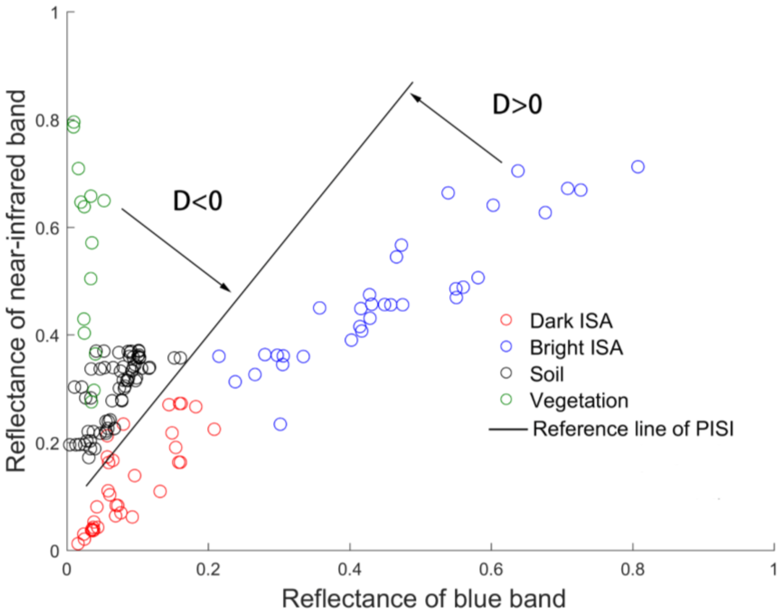
Figure 3 gives a scatter plot of the selected samples in the blue–NIR feature space, where the black solid lines are the dividing lines (not calculated) given by the distribution of scatters. The scatters of the different components demonstrate evident differences in distribution; that is, the ISA scatters are located at the lower right under the soil and vegetation scatters. Therefore, we can distinguish ISA and soil by specifying a dividing line between ISA and soil scatters, as shown in Figure 3. As the vegetation scatters are distributed above the soil scatters, once this dividing line is found, ISA and vegetation are also distinguished.
2.2. PISI Development
According to the spectral features of three main components in the blue–NIR feature space, we selected blue and NIR bands to develop the new index.
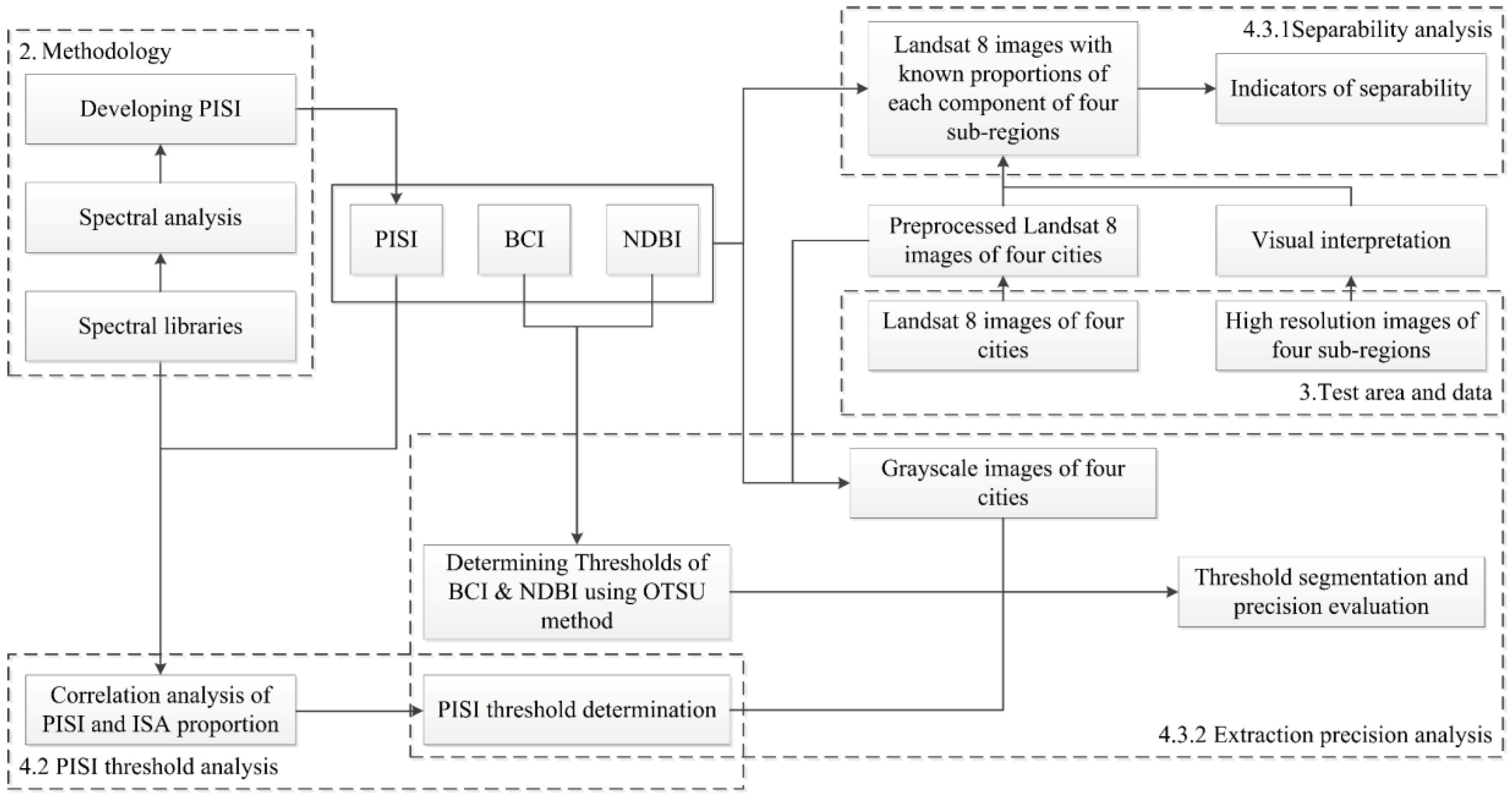
Generally, an index developed by spectral relations can be divided into two categories, ratio form, such as the normalized difference vegetation index (NDVI) [39] and simple ratio [40], and linear form, such as the perpendicular vegetation index (PVI) [41]. The perpendicular index defines a reference line in the feature space, and the perpendicular distance from the point to the reference line is used as the classification basis. According to the concept of the perpendicular index, we can determine a reference line, as shown in Figure 4, so that points below the reference line (i.e., the perpendicular distances are positive) are classified as ISA points, and points above the reference line (i.e., the perpendicular distances are negative) are soil or vegetation points.
Therefore, we used the blue and NIR bands to develop a perpendicular index, and its value represents the perpendicular distance D from the sample point to the reference line (Figure 4). The reference line for PISI is defined as y = ax + b, and and denote the reflectance of blue and NIR bands in blue–NIR feature space, respectively. Then, according to the orthogonal distance formula for the point to the line, D can be obtained as follows:
As PISI is equal to D, we can give the definition of PISI as follows:
According to the definition of PISI, the PISI of the points located in the area between the reference line and the abscissa is greater than 0, whereas the PISI of the points located in the area between the reference line and the ordinate is less than 0. Therefore, our study is aimed at finding the most appropriate reference line to distinguish between ISA and soil (Figure 4). According to the calculation procedure of the soil line in the PVI, the reference line of the PISI can be calculated in the following steps.
2.2.1. Fitting the Soil Line
Take the samples selected from the spectral libraries as an entirety to obtain the fitting line of soil (Figure 5a) in the blue–NIR feature space by least squares linear fitting.
2.2.2. Fitting the ISA Line
If the soil line is regarded as the reference line, the bright ISA sample points and soil can be efficiently separated, but a few dark ISA sample points and some soil sample points are easily confused (as illustrated by a red circle in Figure 5a). As in the case of the soil line, some of the ISA points will be misclassified if the ISA line (Figure 5b) calculated by the ISA point is regarded as a reference line. Therefore, both lines cannot be used as reference lines directly and require further adjustment.
2.2.3. Calculating the Reference Line
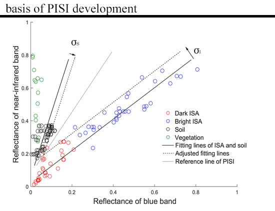
It can be seen in Figure 5b that ISA and soil sample points are distributed on both sides of their corresponding fitting lines. Assuming that the orthogonal distances from a certain category of sample points to their corresponding fitting lines satisfy the normal distribution, the standard deviations of these distances is . Thus, the distances between these sample points and their corresponding fitting line fall mostly into [, ]. Therefore, with and defined as the standard deviations of the orthogonal distances between the soil and ISA sample points and their corresponding fitting lines, we adjusted the fitting line of soil by moving it in parallel in an orthogonal direction, as shown in Figure 5c, with a distance of , and the adjusted ISA line can also be obtained with the same procedure. After being adjusted, most of the soil sample points are located at the upper left and most of the ISA sample points are located at the lower right of the adjusted ISA line. Furthermore, the bisector of the angle between the two adjusted lines is considered as the reference line of the PISI (Figure 5d).
The parameters of the reference line of the PISI can be calculated as follows:
The soil line equation is assumed to be y = x + , the ISA line equation is y = , the adjusted soil line equation is , and the adjusted ISA line equation is given the parallel movement. Then, and can be obtained as follows:
assuming are the orthogonal distances from a point located on the reference line of the PISI to the adjusted ISA line and soil line, respectively. Therefore, the reference line of the PISI satisfies the following equation:
The distance equation is then integrated into Equation (4) as follows:
By defining and , Equation (5) can be simplified as follows:
Therefore, coefficients a and b of the reference line of the PISI are obtained as follows:
Equation (3) is substituted into Equation (7) as follows:
Then, a and b are integrated into Equation (2), and the coefficient of the PISI can be calculated. According the ISA and soil samples selected from the spectral libraries, the formulas for the fitting lines of ISA and soil are y = 0.8863x + 0.0428 (R2 = 0.9089) and y = 2.5325x + 0.0520 (R2 = 0.8209) and the standard deviations of ISA and soil are = 0.2081 and = 0.1606, and, finally, the formula for PISI can be obtained via the above formulas:
3. Test Area and Data
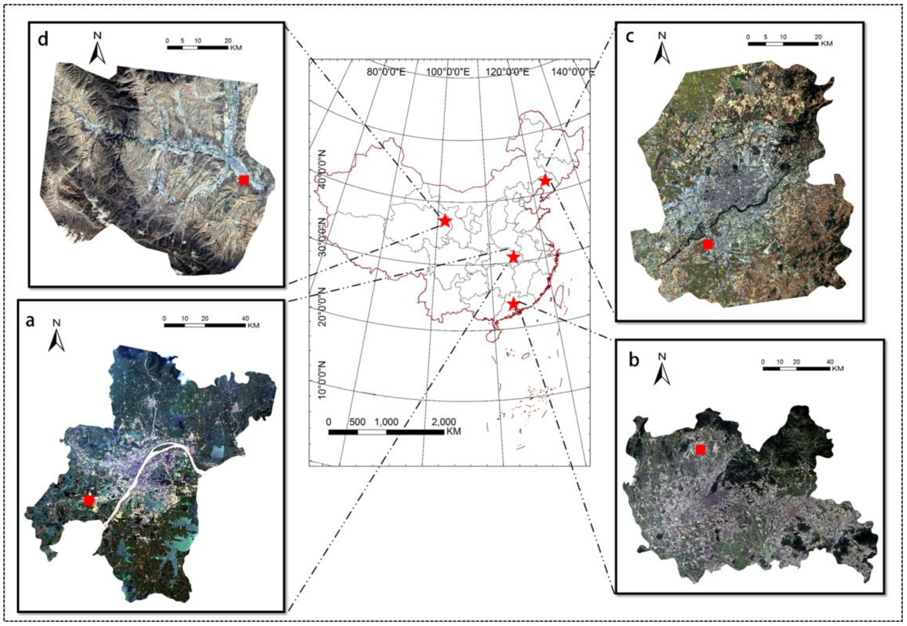
Landsat 8 images were used in this study as the test data for the PISI in medium-resolution remotely sensed images. Four cities in China—Wuhan, Guangzhou, Shenyang, and Xining—were selected as test areas (Figure 6). Wuhan (30.52°N, 114.31°E), the center city of central China, is the largest inland transport hub, with numerous lakes and a humid subtropical monsoon climate. Guangzhou (23.12°N, 113.35°E) is located in the subtropical coast and is the center city in southern China; this city has a developed economy and a subtropical monsoon climate, with an urbanization rate of more than 80%. Shenyang (41.8°N, 123.38°E) is an important industrial base in northeastern China with a high degree of urbanization, where the terrain is dominated by plains, and it has a temperate semi-humid continental climate. Xining (36.56°N, 101.74°E), which is located in northwest China, is one of the highest-altitude cities in the world, with a continental arid–semiarid climate and surrounded by mountains. These four cities, located in the northwestern, northeastern, central, and southern areas of China, have a large span of space, covering a wide range (23.12°N–41.8°N, 23.12°E–123.38°E), and have different geographic environments and climates. These cities can be used to verify the applicability of the PISI under different experimental conditions. Taking the influence of cloud amount into account, the acquisition dates of the Landsat 8 images were 31 July 2013 (Wuhan), 18 October 2015 (Guangzhou), 29 September 2016 (Shenyang), and 10 May 2016 (Xining). Atmospheric correction and water removal were carried out before PISI calculation by using the ENVI FLAASH module and the modified normalized difference water index (MNDWI) [42], respectively. Related calculations in subsequent experiments were done using MATLAB and ENVI software.
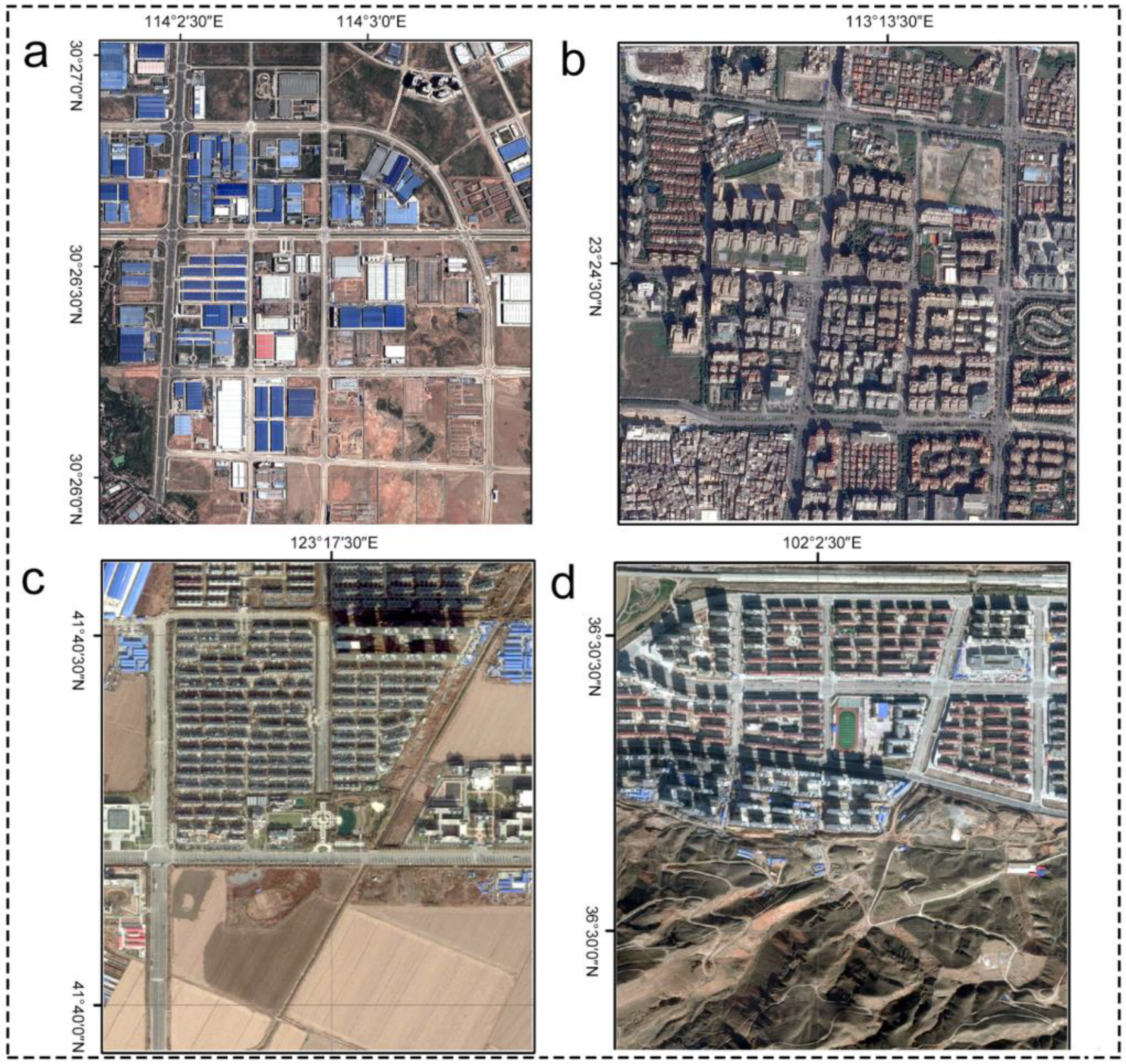
In subsequent sections, the exact proportions of ISA, soil, and vegetation in Landsat 8 images are acquired, as shown in Figure 7. We selected four high-resolution images with 1.07 m spatial resolution of representative subregions (red rectangle in Figure 6) from Google Earth software, and the acquisition times were approximately consistent with the corresponding Landsat 8 images. Part a was selected from Wuhan, with a large amount of soil and minimal vegetation and buildings. Part b was selected from Guangzhou, with buildings and roads as the main land cover types. Part c was selected from Shenyang, where most of the vegetation in the experimental area was withered and the fields were bare soil. Part d was selected from Xining, with a residential district, vegetation dominated by sparse shrubs, and mountains. The acquisition dates for the four subregions were: 7 May 2013 (Part a), 19 December 2015 (Part b), 13 November 2016 (Part c), and 4 November 2016 (Part d). The high-resolution images were classified into ISA, soil, and vegetation by visual interpretation, and the results were regarded as the ground truth to obtain the proportion of each component in the corresponding region of Landsat 8 images.
4. Results
4.1. Applying PISI to Landsat 8 Images
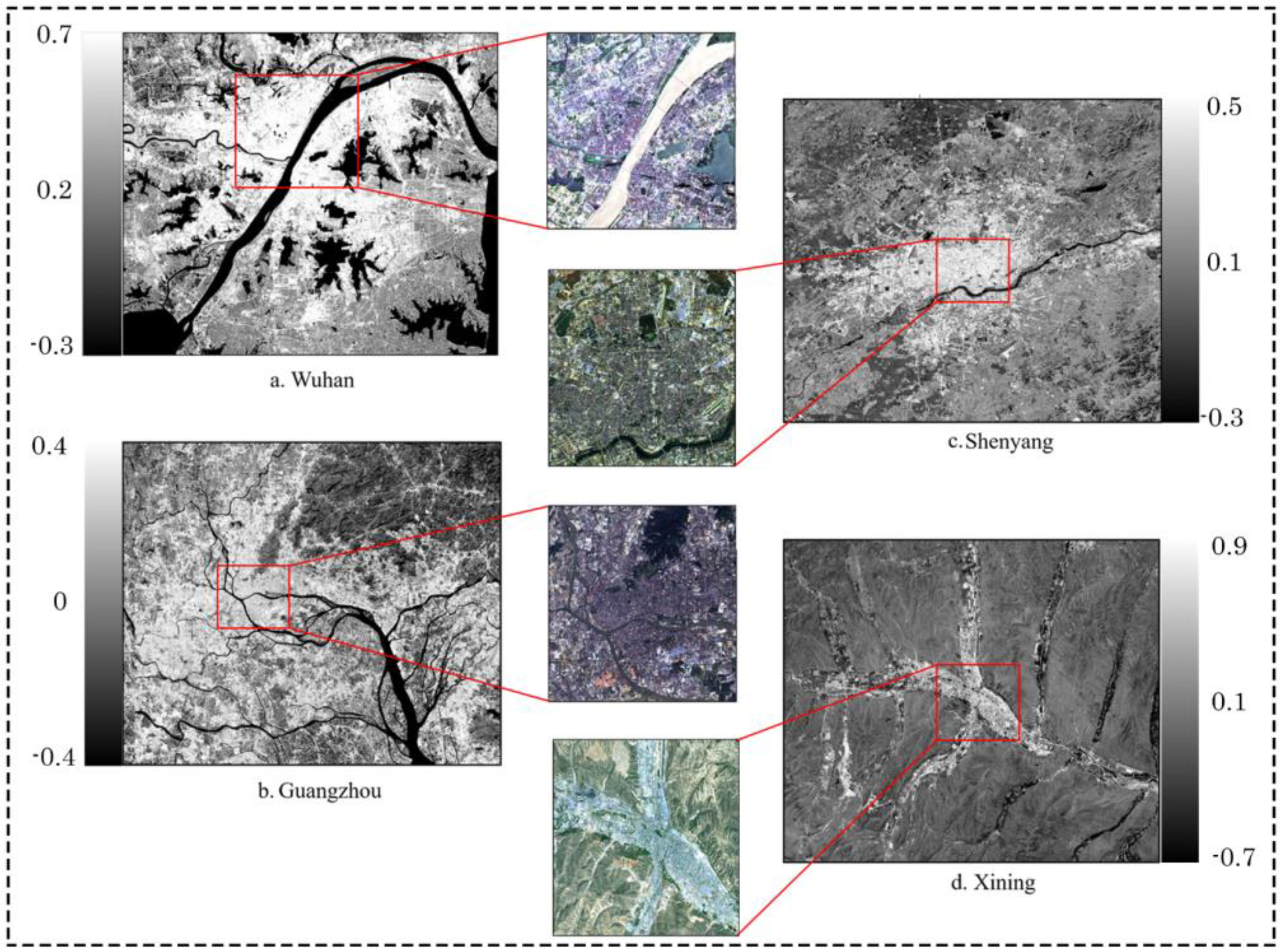
We first applied PISI to the Landsat 8 images of Wuhan, Shenyang, Guangzhou, and Xining. The results of the four cities are shown in both sides of Figure 8. Clearly, significant differences exist in the brightness of the three components. Among the three components, ISA has the highest brightness with a white tone, followed by soil, which shows a gray tone. Vegetation has the lowest brightness and negative values, with a partial black tone.
4.2. PISI Threshold Analysis
4.2.1. Correlation Analysis of PISI and ISA Proportions
Mixed pixels are common in Landsat 8 images. Actually, a pixel may contain multiple types of land cover and the spectra of these components vary widely. Obviously, the proportions of ISA, soil, and vegetation have a significant impact on PISI value. Therefore, a simulation experiment was conducted by using the spectral libraries to analyze the impact of different proportions of background (soil and vegetation) and ISA on PISI. The simulation experiment satisfies the following assumptions: (1) only three components, ISA, vegetation, and soil, exist in urban scenes; (2) the remotely sensed images were unaffected by the atmosphere or were subjected to atmospheric correction; and (3) the spectra of pixels can be obtained by linearly mixing the spectra of the three components according to a certain proportion, and the spectra of ISA, vegetation, and soil used for the simulation experiment are expressed by the average of ISA, vegetation, and soil samples selected from the spectral libraries, respectively. Specifically, the soil proportion in the background does not exceed 0.5. These assumptions satisfy the following equations:
where represents the reflectance of the background, which comprises soil and vegetation; is the reflectance of the mixed pixels; , , and represent the reflectance of ISA, soil, and vegetation, respectively, obtained from the spectral libraries; and , , , and are the proportions of ISA, soil, vegetation, and , respectively. Therefore, the pixels were obtained by mixing the spectra of ISA, soil, and vegetation in accordance with a certain proportion. We considered six background cases, that is, the combination of soil and vegetation where soil coverage is 0%, 10%, 20%, 30%, 40%, or 50%, in accordance with the assumptions.
In terms of the simulation results, Figure 9 shows the PISI values with different proportions of ISA in six simulation cases, where the abscissa indicates the ISA proportion and the ordinate represents the PISI value. In general, the value of PISI increases with the proportion of ISA under six simulation conditions, showing a positive correlation, and the range of PISI is [−0.1265, 0.1462]. Meanwhile, considering the same ISA proportions, low ISA proportions are linked to a greater variance of the PISI index, and this variance gets smaller when the ISA percentage rises, which is also in line with common sense. The larger the ISA proportion, the smaller the corresponding PISI change and the more reliably it can be regarded as the ISA pixel. However, the PISI value increases from −0.1265 to −0.0558 when the ISA coverage equals 0. Therefore, a pixel with PISI value falling in this range should be considered an “uncertain” category, because this pixel can be determined by either ISA or background or both. Meanwhile, when taking −0.0558 as the lower threshold, for the most extreme case where the proportion of soil is 0, the corresponding proportion of ISA is 0.26. That is, when the proportion of ISA is greater than 0.26, the PISI value must fall into the range of [−0.0558, 0.1462] regardless of the composition of the background, and [−0.0558, 0.1462] can be considered as the threshold of PISI.
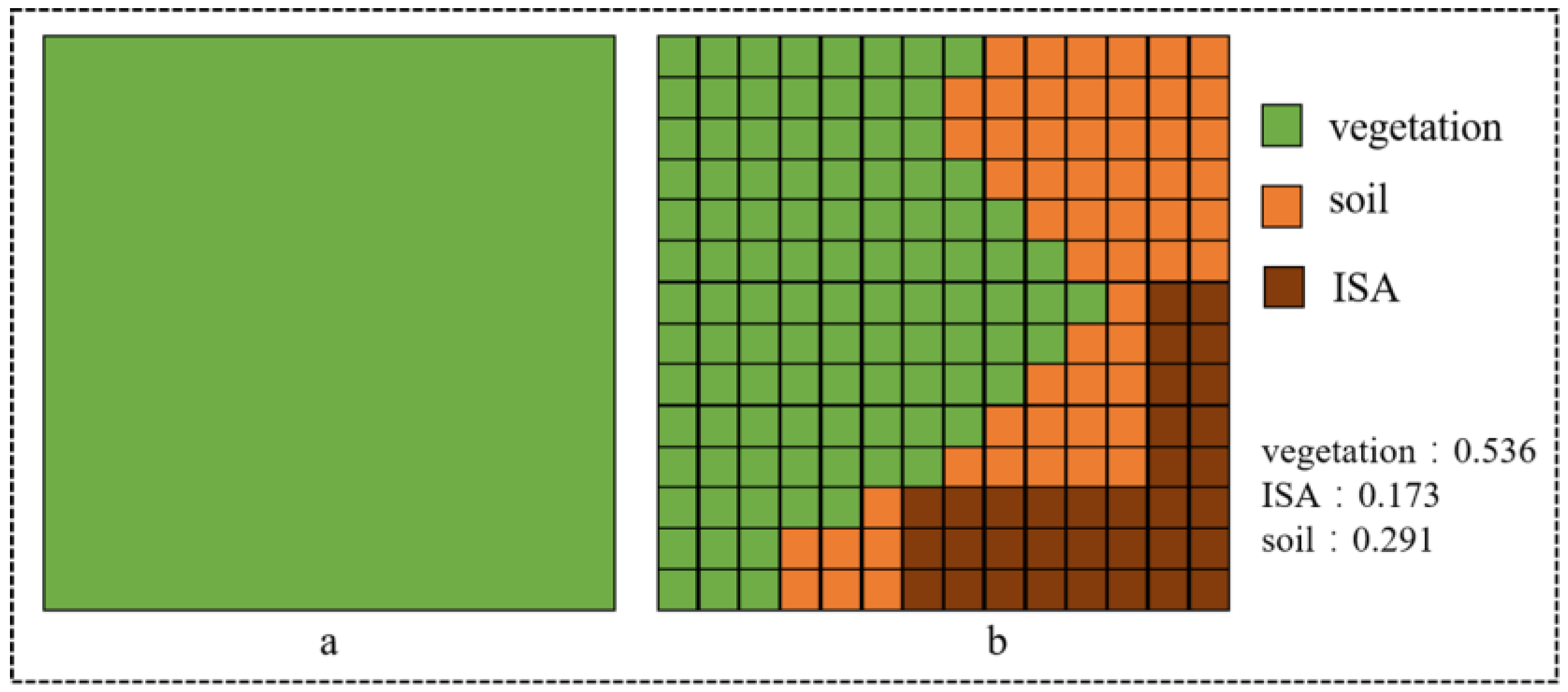
However, the above is just a simulated situation; in practice, since the spectra of ISA, soil, and vegetation in Landsat 8 images have a certain degree of heterogeneity, for pixels with the same ISA proportion, both the different background composition and the different specific categories of ISA and background make the value of PISI change greatly, so we conducted an experiment to analyze the correlation between PISI and ISA proportion in pixels of Landsat 8 images. The four subregions were taken as test areas in this section, and the visual interpretation results of high-resolution images were used to calculate the proportion of each component (ISA, soil, and vegetation) in each pixel of the corresponding Landsat 8 images (Figure 10). Therefore, for proportion p, we can get N pixels with ISA proportion equal to p, and among the N pixels, the PISI value of pixel i is PISIpi. Then, we took the average PISI of all pixels with the same ISA proportion for analysis to eliminate the effects of heterogeneity:
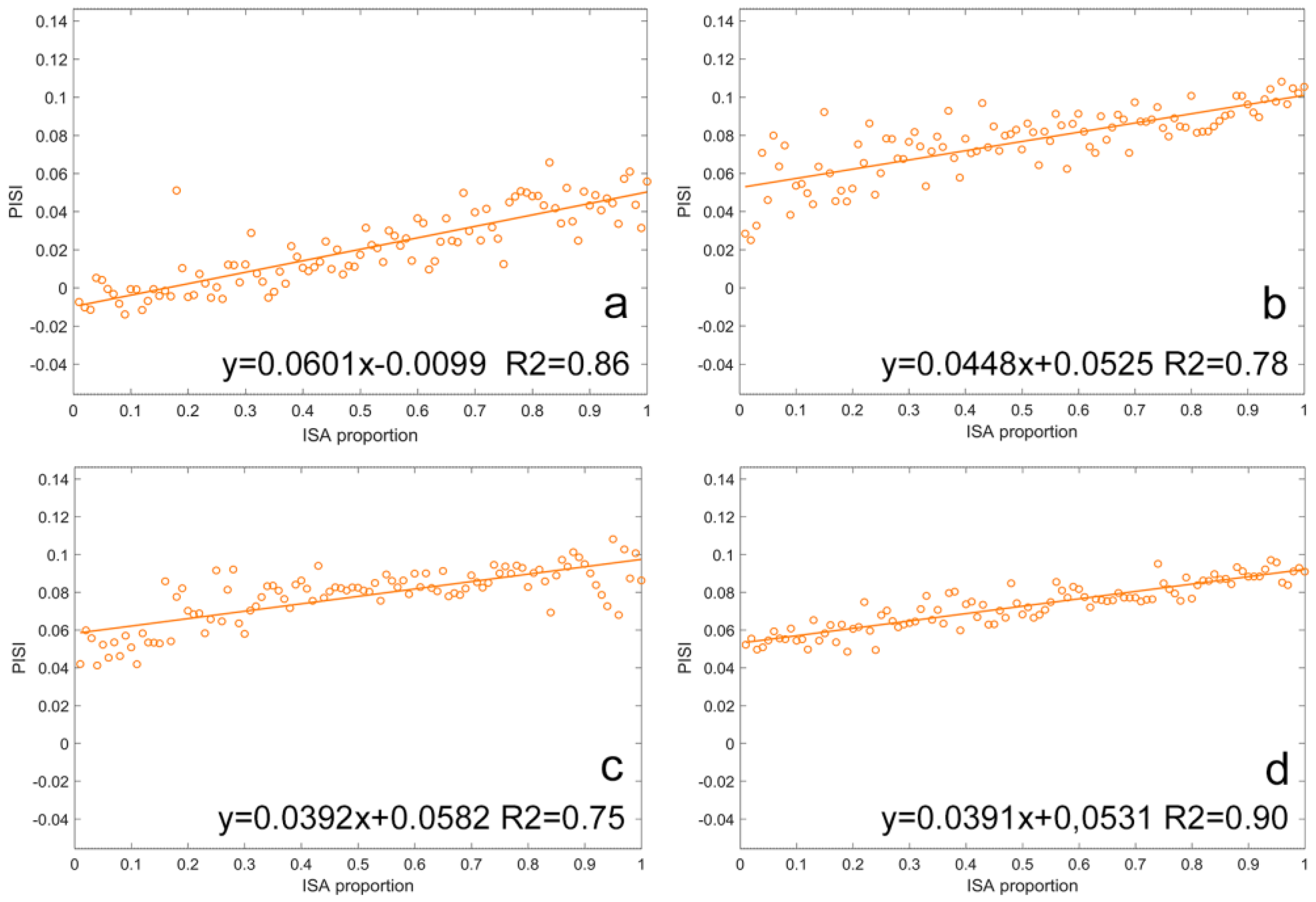
In this way, we performed a correlation analysis on the Landsat 8 pixels of the four subregions (Figure 11). Obviously, the PISI value is also positively correlated with ISA proportion, and the correlation coefficients of the four subregions are 0.86, 0.78, 0.75, and 0.90. At the same time, the PISI values of Landsat 8 pixels are also distributed within [−0.1265, 0.1462], which is also consistent with the above simulation experiment. Therefore, the conclusions we obtained in the simulation experiment can be extended to practical applications.
4.2.2. PISI Threshold Determination
In threshold segmentation, as the real category of each pixel in Landsat 8 images needs to be classified into ISA or non-ISA, it matters how much of the proportion of ISA is reached to classify the pixel into this category, namely, the threshold of ISA proportion. For this reason, we did another experiment to verify the effect of ISA proportion threshold on accuracy, and the test data were the Landsat 8 images of the four subregions with known component proportions.
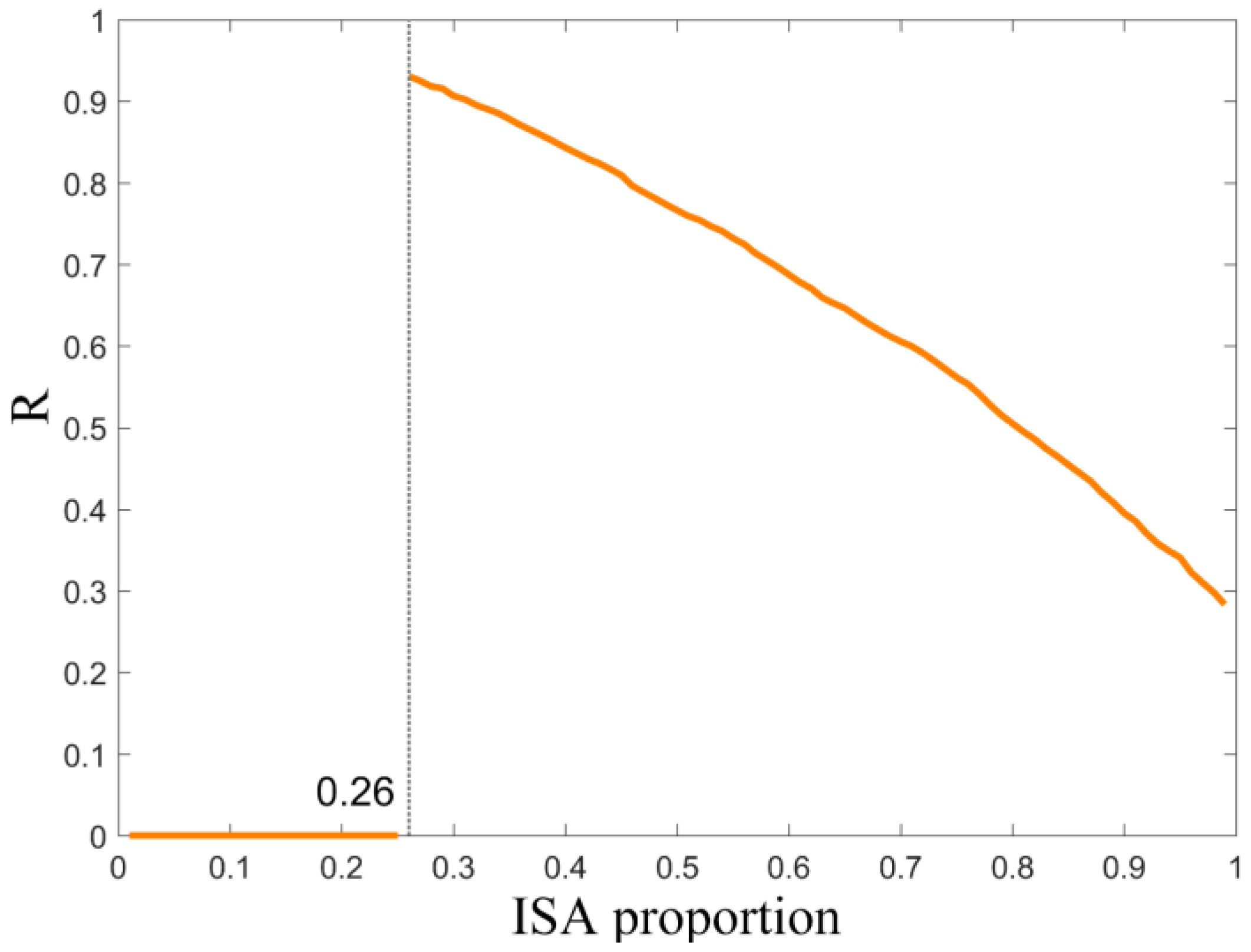
We assumed that pixels whose ISA proportions are greater than X are ISA pixels and those less than X are non-ISA pixels, and counted the number of ISA pixels, denoted as A. Then, the image was segmented according to the PISI threshold [−0.0558, 0.1462] obtained from the simulation experiment, and the number of pixels classified as ISA according to the threshold was denoted as B. We used R = A/B to measure the effect of ISA proportion threshold on accuracy. To verify the conclusion obtained in the simulation experiment, i.e., that when the ISA proportion is greater than 0.26, the corresponding PISI value falls within [−0.0558, 0.1462], the starting value of X is 0.26. As shown in Figure 12, when the proportion of ISA is less than 0.26, R = 0; when X = 0.26, the corresponding R = 0.94; and when X = 0.34 (1/3), R = 0.89. The results show that the proportion threshold of ISA has a significant impact on accuracy, and as the threshold increases, the accuracy decreases. However, according to the simulation experiment, as the threshold of ISA proportion changes, the threshold of PISI should also change. Therefore, we did another set of experiments.
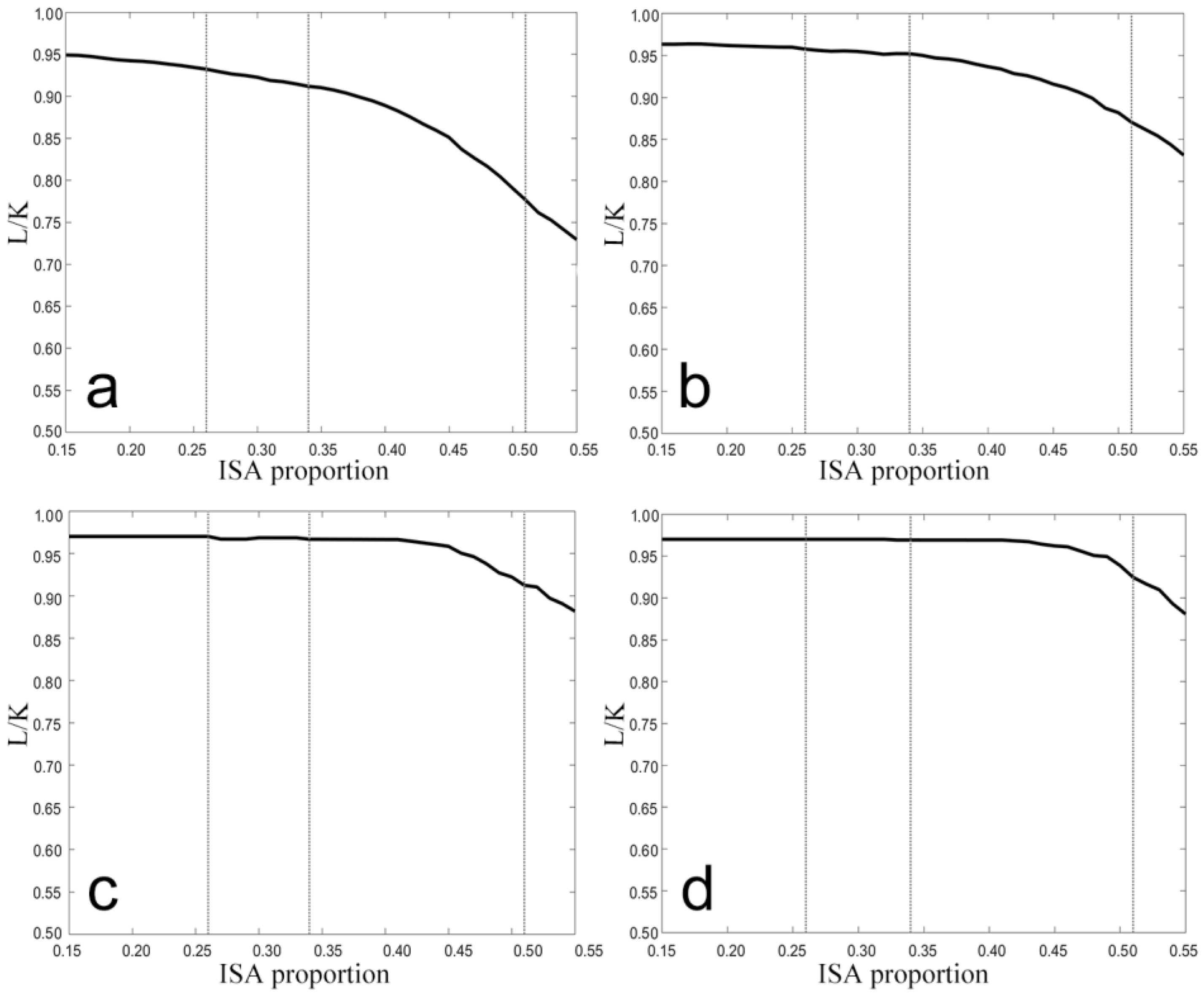
We assumed the criterion for determining whether a pixel is an ISA pixel as an ISA proportion greater than Y, and the corresponding threshold for Y in the simulation experiment is [a, 0.1462] (a can be obtained from the simulation experiment). We then used Y to classify one Landsat 8 image, and the total number of ISA pixels obtained is K. Among these K pixels, the number whose corresponding PISI values are distributed within [a, 0.1462] range is L. If the results of the classification based on ISA proportion are consistent with the classification based on PISI threshold segmentation, L/K should be close to 1. As shown in Figure 13, we verified this assumption in four subregions: the black lines represent L/K and the horizontal axis represents the ISA proportion threshold with a range [0.15, 0.55]. We also list key values of ISA proportion (e.g., 0.26, 0.34, and 0.51) in Table 1.
As shown in Figure 13, the black lines are still at a high level with increased ISA proportion, indicating that the PISI threshold itself has good self-adaptability to different proportions of ISA in Landsat 8 pixels. It should be noted that, according to Table 1, the different ISA proportion thresholds have a significant impact on accuracy and need to be adjusted according to the actual situation. In summary, PISI can be used in practice in two ways with different accuracy: (1) in cities, where the area with an ISA proportion greater than a specified value, for example a PISI threshold of [−0.0558, 0.1462] if one wants to know the area where the proportion is greater than 0.26; and (2) obtaining a reliable area of ISA. To achieve this purpose, one needs to define the threshold of ISA proportion.
4.3. Comparative Analyses with Other Indices
4.3.1. Separability Analysis with Other Indices
Separability analysis was designed to test the ability of the three indices to distinguish the three components. In detail, high-resolution images of the four subregions were classified into ISA, soil, and vegetation pixels by visual interpretation to get accurate ISA, soil, and vegetation proportions of Landsat 8 image pixels. Then, the pixels of the Landsat 8 images were classified into ISA, soil, and vegetation based on the dominant component. PISI, BCI, and NDBI were then applied to the images of the four subregions to get grayscale images. That way, each index obtained pixel sets representing ISA, soil, and vegetation from the grayscale images of each subregion. Referring to the separability analysis in BCI [35], i and j are two of the three components (e.g., ISA and soil, or ISA and vegetation), is the average value, is the standard deviation, c is the covariance (in this experiment, the input was single-band data and the covariance was variance), and is the trace of matrix. The spectral discrimination index (SDI) [43,44], Jeffries-Matusita (J-M) distance [45], and transformed divergence (TD) [46] were then used to measure the separability of ISA and soil and ISA and vegetation (Figure 12). The formulas for SDI, J-M distance, and TD are as follows:
where is:
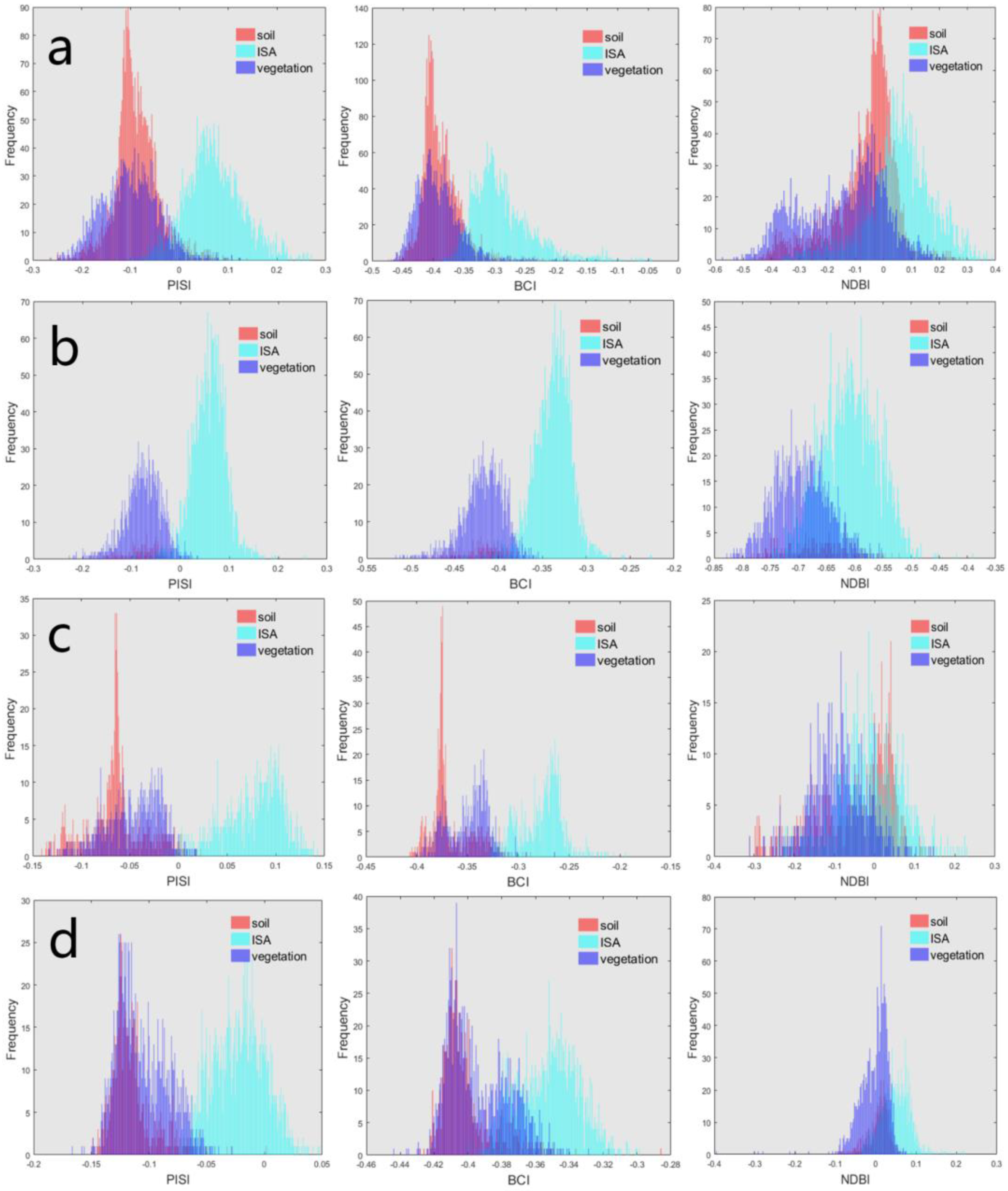
As described above, Figure 14 demonstrate frequency histograms of the values by applying PISI, BCI, and NDBI to the Landsat 8 images of the four subregions. Separability is evaluated by using SDI, J-M distance, and TD.
In Figure 14 and Table 2, PISI is of the optimal separability between ISA and other components, and NDBI is the worst. In areas where ISA is the main ground cover type, e.g., Part b, with minimal bare soil, the separability of the PISI is slightly higher than the BCI. However, in areas where there is a lot of bare soil, e.g., Parts a and c, which makes it difficult for ISA extraction, PISI has obvious advantages compared to the other two indices. It is worth noting that Part d is covered by mountains and sparse shrub. In this area, BCI and NDBI performed less satisfactorily.
4.3.2. Extraction Precision Analysis with Other Indices
In the extraction accuracy analysis, the three indices were first applied to the Landsat 8 images of the four cities to obtain the corresponding grayscale images, and then the binary images of ISA distribution were obtained through the respective thresholds of the three methods (Figure 15). It should be noted that we selected [−0.0558, 0.1462] as the threshold of PISI, and the thresholds of BCI and NDBI were not specified in the original papers, so their initial thresholds were calculated by Otsu’s method, and we used this as a basis to adjust and determine the optimal thresholds. The definition of Otsu’s method is as follows:
For grayscale image I, the segmentation threshold of the foreground (i.e., ISA) and background (i.e., soil and vegetation) is denoted as T, the percent of pixels belonging to the foreground occupying the entire image is denoted as , and the average grayscale is . The percent of background pixels in the entire image is and the average grayscale is . The total average grayscale of the whole image is denoted as μ, and the variance between classes is denoted as g. Assuming that the background of the image is darker than the foreground and the size of the image is M × N, the number of pixels whose gray value is greater than threshold T is denoted as , and the number of pixels whose gray value is less than threshold T is denoted as . We can get the following formula:
Substituting Equation (20) into Equation (21) yields the equivalent formula:
Then, the traversal method is used to obtain the T that maximizes the g, which is the required threshold. Normally, Otsu’s method requires a set of positive integers with bimodal intensity distributions, and the histograms of the four subregions satisfy this requirement (Figure 14). However, the inputs of this experiment are non-integer and some are even negative. Therefore, the original data need to be transformed. For input set S, its threshold satisfies the following formula [47]:
where OTSU () indicates the threshold obtained by Otsu’s method, [] is the rounding operator, and a and b are parameters that guarantee + b is a positive integer set.
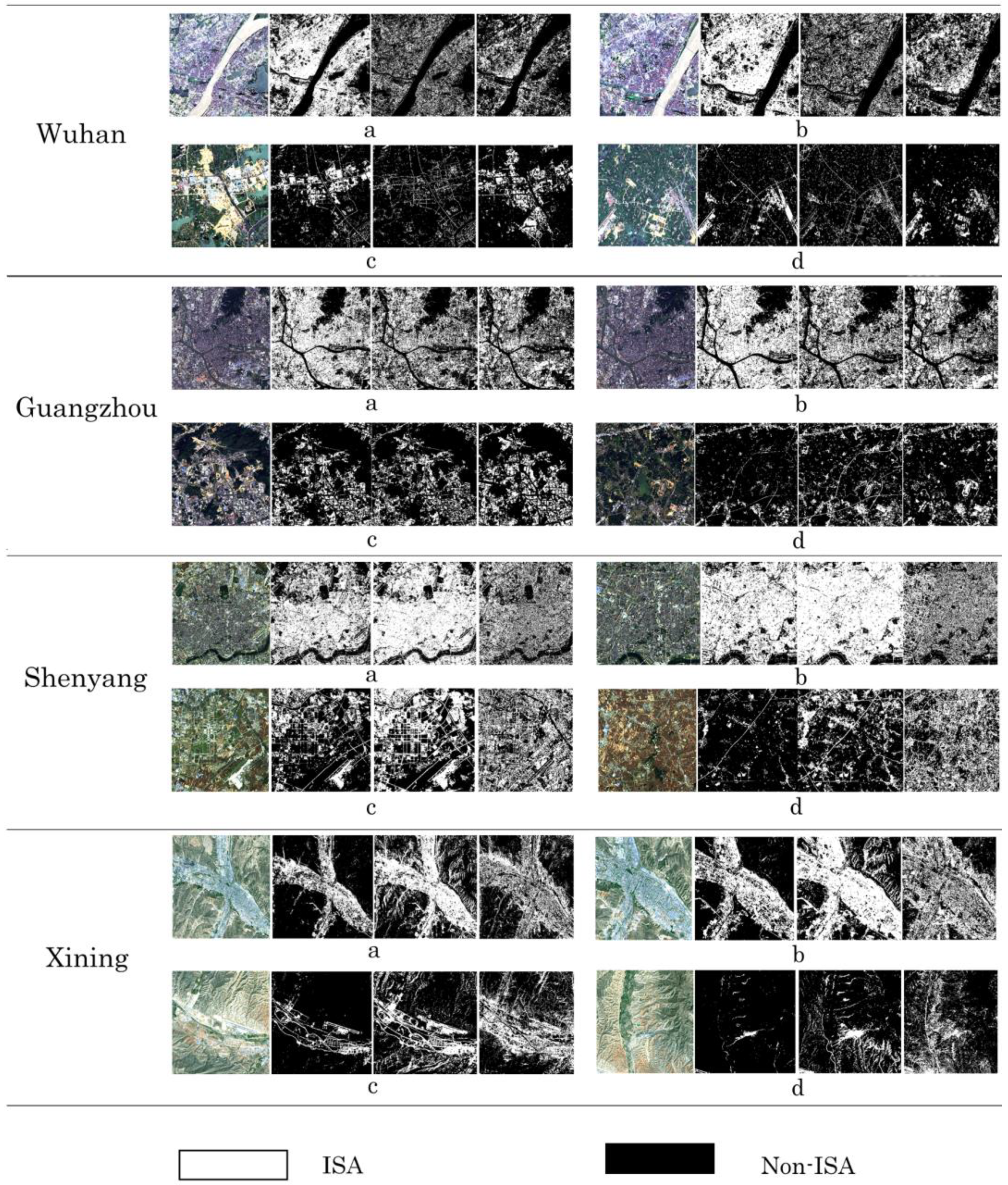
Thresholds of PISI, BCI, and NDBI were applied to the grayscale images (Figure 8), where pixels with values falling in corresponding thresholds were classified as ISA and reassigned 1, and pixels with values out of this range were classified as soil or vegetation and reassigned a value of 0 to obtain the segmentation images. Figure 15a–d in each city indicates the extraction results in the corresponding city under the overall, urban, suburban, and rural scenes, respectively. In each unit, from left to right are the true-color composite images and the results of ISA extraction using PISI, BCI, and NDBI. Then, samples were evenly selected from overall scenes to obtain confusion matrices, and the overall accuracy and kappa coefficient (shown in Table 3) were used to measure the extraction accuracy of PISI, BCI, and NDBI.
In Figure 15, it is clear that the bright area is the ISA, where soil and vegetation are removed, compared with the Landsat 8 true-color images. In addition, the shape and integrity of the ISA also achieve a favorable reservation.
Combining Figure 15 and Table 3 for analysis, we can see the following: (1) PISI can achieve the highest classification accuracy among the three indices, except in Guangzhou where the accuracy is less than 90%, and the NDBI exhibits the worst performance; (2) The suburban scene is the urban–rural frontier, and the land cover types are complex and mainly contain construction, farmland, vegetation, and soil. As displayed in Figure 15 (Shenyang, Figure 15c), BCI and NDBI easily divide soil into ISA; (3) In addition to soil, farmland and mountains also affect the extraction of ISA. The spectral curves of upland fields and soil are also partially similar. Hence, farmland can be easily classified as ISA (Shenyang, Figure 15d). The BCI is sensitive to water, and the extraction results of BCI in the suburban and rural scenes are not sufficiently good, especially in the rural area of Wuhan (Wuhan, Figure 15d), where many paddy fields exist. Xining is surrounded by mountains. The BCI and NDBI divided mountains into ISA (Xining, Figure 15a–d), whereas the PISI can remove mountains well.
5. Discussion
The present study proposes an index that eliminates or reduces soil and vegetation interference to ensure that the PISI has high accuracy for ISA extraction at medium-resolution remotely sensed images in different scenes.
Obviously, the PISI has satisfactory performance and is a potential index. Its advantages are that it has better performance in both separability and ISA extraction precision, especially in areas with more soil. Second, as there is a significant positive correlation between PISI and ISA proportion, PISI can adjust its threshold to get the area where the ISA proportion is greater than a specified value, or obtain reliable ISA area by defining the threshold of ISA proportion. In addition, PISI only needs very common blue and near infrared bands. Therefore, it can be used in more scenarios.
However, some aspects need to be discussed. First, the samples selected from the spectral libraries are single pure samples (paints, metal materials, concrete, asphalt, and plastic). Although these samples can eliminate the influence of mixed pixels and subjective factors when they are selected directly from the images, they cannot fully express real city scenes. Second, the proportions of ISA, soil, and vegetation in pixels of Landsat 8 images need to be obtained for the experiment. Several methods [48,49] can achieve this goal. However, these methods are limited by image resolution and have difficulty achieving accurate results even with the SMA-based methods. Therefore, high-resolution images of the four subregions (Figure 7) with 1.07 m resolution were selected to obtain the accurate proportions of ISA, vegetation, and soil in each pixel of the corresponding Landsat 8 images by visual interpretation (Figure 10). Third, studies show that the extraction precision of ISA is also influenced by factors such as season, and summer images are the most suitable for ISA extraction [50,51]. However, the criterion we chose for the experimental areas was large differences that exist in the geographic environment to test the performance of PISI under different circumstances, and four Chinese cities—Wuhan, Guangzhou, Shenyang, and Xining—were selected. Then, as the amount of cloud is a main consideration, images of the four cities were acquired in different seasons. Apart from season, soil moisture is another factor that affects accuracy. Broadly speaking, reflectance of soil decreases with increasing water content, with the effect more pronounced at longer wavelengths [52]. Moreover, ground-based techniques [53] and microwave remote sensing [54] are the most commonly used methods for soil water content measurement, but these data are not readily available. From a macro perspective, of the four cities we selected, Xining is in a high-latitude and high-altitude mountainous area and Shenyang is at a high latitude and its image acquisition time was autumn, so the precipitation of these two cities was less. In contrast, the precipitation in Wuhan in summer and in Guangzhou, a coastal city, was relatively large. Therefore, these two pairs of cities can reflect the applicability of PISI in different soil moisture areas to some extent. However, more rigorous experimentation is needed. Fourth, high-resolution remote sensing images are more accessible than before with the continuous improvement of satellite sensor resolution. Therefore, the PISI was also applied to the Worldview 3 image of Zigui County, Hubei Province, China, which is a new city built for immigrants of the Three Gorges Project. In Figure 16, the true color composite image is on the left, and the threshold segmentation image by PISI is on the right. The visual result illustrates that the PISI still has excellent potential for high-resolution images.
6. Conclusions
In recent years, ISA has emerged not only as a feature of urbanization but also as a major index of environmental quality. The accurate extraction of ISA is crucial to municipal construction, city planning, sustainable development, and ecological assessment. Among existing methods, such as mixture analysis methods and classification-based methods, the former rely heavily on the quality of the endmember, and in some methods of this category, the process to acquire the endmember is very complicated. For the latter, they need high-quality training data. In contrast, the index-based methods are easy to implement and their accuracy is acceptable.
The challenges in ISA extraction are that ISA and soil are easily confused with each other. Furthermore, the heterogeneity of ISA also affects the extraction results. To address these challenges, based on a VIS model, we analyzed the spectral curves of ISA, soil, and vegetation. Keeping in mind the effects of mixed pixels and the atmosphere, the spectral curves of ISA, soil, and vegetation were selected from the spectral libraries, and they have obvious differences in the reflectance of the blue and NIR bands (Figure 2 and Figure 3). Therefore, the two bands were selected to develop the PISI, and the parameters of the PISI were obtained by using the samples of the spectral libraries. Meanwhile, Landsat 8 images of four Chinese cities and high-resolution images of four subregions were taken as test data. In the PISI threshold analysis, the relationship of PISI and ISA proportion was examined, showing a high positive correlation (Figure 11). Then, the effect of PISI threshold on ISA extraction accuracy was considered (Figure 13), indicating that the PISI threshold can be adjusted according to actual needs with different accuracy. In comparative analysis, results show that PISI has optimal separability compared to other indices in four subregions (Figure 14) and better performance than BCI and NDBI in ISA extraction (Figure 15 and Table 3).
Three conclusions can be drawn from this study. First, compared to other indexes, PISI has less stringent requirements for data. The data sources required for PISI are only the blue and NIR bands, which are common to most satellite sensors. By contrast, mid-infrared bands required by NDBI and tassel cap and transformation matrix required by BCI are not available from some sensors. Second, PISI is more flexible to use. As PISI has a significant positive correlation with ISA proportion, the threshold can be adjusted according to actual needs. Moreover, because the parameters of PISI were calculated from samples in the spectral libraries, they can be adjusted by updating the spectral libraries. Third, with higher ISA extraction precision and better separability of ISA and soil and ISA and vegetation, PISI is a more reliable index.
Author Contributions
Y.T. acquired the data, analyzed the results, and reviewed the original draft. H.C., conducted the investigation, conceived the methodology, visualized relevant results, and drafted the original draft. Q.S. processed data curation and validation. K.Z. acquired funding. The manuscript was improved with contributions from all co-authors.
Funding
The research in this paper was supported by National Key Research and Development Program (Grant No. 2018YFB1004600) and partly supported by National Key Research and Development Program (Grant No. 2016YFB0502603).
Acknowledgments
The authors are grateful to the editors, anonymous reviewers and professor Jin Chen at Beijing normal university for their critical comments and valuable suggestions, which helped to improve the quality of this manuscript substantially.
Conflicts of Interest
The authors declare no conflict of interest.
References
- White, M.D.; Greer, K.A. The effects of watershed urbanization on the stream hydrology and riparian vegetation of Los Peñasquitos Creek, California. Landsc. Urban Plan. 2006, 74, 125–138. [Google Scholar] [CrossRef]
- Schueler, T.R. The Importance of Imperviousness. Water Prot. Tech. 1994, 1, 100–111. [Google Scholar]
- Oke, T.R. The energetic basis of the urban heat island. Q. J. R. Meteorol. Soc. 2006, 108, 1–24. [Google Scholar] [CrossRef]
- Xian, G.; Crane, M. An analysis of urban thermal characteristics and associated land cover in Tampa Bay and Las Vegas using Landsat satellite data. Remote Sens. Environ. 2006, 104, 147–156. [Google Scholar] [CrossRef]
- Yuan, F.; Bauer, M.E. Comparison of impervious surface area and normalized difference vegetation index as indicators of surface urban heat island effects in Landsat imagery. Remote Sens. Environ. 2007, 106, 375–386. [Google Scholar] [CrossRef]
- Coseo, P.; Larsen, L. How factors of land use/land cover, building configuration, and adjacent heat sources and sinks explain Urban Heat Islands in Chicago. Landsc. Urban Plan. 2014, 125, 117–129. [Google Scholar] [CrossRef]
- Huang, F.; Zhan, W.; Voogt, J. Temporal upscaling of surface urban heat island by incorporating an annual temperature cycle model: A tale of two cities. Remote Sens. Environ. 2016, 186, 1–12. [Google Scholar] [CrossRef]
- Weng, Q. Remote sensing of impervious surfaces in the urban areas: Requirements, methods, and trends. Remote Sens. Environ. 2012, 117, 34–49. [Google Scholar] [CrossRef]
- Harbor, J.M. A Practical Method for Estimating the Impact of Land-Use Change on Surface Runoff, Groundwater Recharge and Wetland Hydrology. J. Am. Plan. Assoc. 1994, 60, 95–108. [Google Scholar] [CrossRef]
- Arnold, C.L., Jr.; Gibbons, C.J. Impervious Surface Coverage: The Emergence of a Key Environmental Indicator. J. Am. Plan. Assoc. 1996, 62, 243–258. [Google Scholar] [CrossRef]
- Vogelmann, J.E.; Howard, S.M.; Yang, L.M. Completion of the 1990s National Land Cover Data Set for the Conterminous United States From LandSat Thematic Mapper Data and Ancillary Data Sources. Photogramm. Eng. Remote Sens. 2001, 67, 650–662. [Google Scholar] [CrossRef]
- Homer, C.H.; Fry, J.A.; Barnes, C.A. The National Land Cover Database. US Geological Survey Fact Sheet. 2012, 3020, 1–4. [Google Scholar]
- Song, X. Characterizing the magnitude, timing and duration of urban growth from time series of Landsat-based estimates of impervious cover. Remote Sens. Environ. 2016, 175, 1–13. [Google Scholar] [CrossRef]
- Kotarba, A.Z.; Aleksandrowicz, S. Impervious surface detection with nighttime photography from the International Space Station. Remote Sens. Environ. 2016, 176, 295–307. [Google Scholar] [CrossRef]
- Masek, J.G.; Lindsay, F.E.; Goward, S.N. Dynamics of urban growth in the Washington DC metropolitan area, 1973-1996, from Landsat observations. Int. J. Remote Sens. 2000, 21, 3473–3486. [Google Scholar] [CrossRef]
- Shi, L.F.; Ling, F.; Ge, Y. Impervious Surface Change Mapping with an Uncertainty-Based Spatial-Temporal Consistency Model: A Case Study in Wuhan City Using Landsat Time-Series Datasets from 1987 to 2016. Remote Sens. 2017, 9, 1148. [Google Scholar] [CrossRef]
- Hu, X.; Weng, Q. Estimating impervious surfaces from medium spatial resolution imagery using the self-organizing map and multi-layer perceptron neural networks. Remote Sens. Environ. 2009, 113, 2089–2102. [Google Scholar] [CrossRef]
- Zhang, Y.; Zhang, H.; Lin, H. Improving the impervious surface estimation with combined use of optical and SAR remote sensing images. Remote Sens. Environ. 2014, 141, 155–167. [Google Scholar] [CrossRef]
- Zhou, Y.; Wang, Y.Q. Extraction of Impervious Surface Areas from High Spatial Resolution Imagery by Multiple Agent Segmentation and Classification. Photogramm. Eng. Remote Sens. 2015, 74, 857–868. [Google Scholar] [CrossRef]
- Zhang, X.; Du, S. A Linear Dirichlet Mixture Model for decomposing scenes: Application to analyzing urban functional zonings. Remote Sens. Environ. 2015, 169, 37–49. [Google Scholar] [CrossRef]
- Small, C.; Lu, J.W.T. Estimation and vicarious validation of urban vegetation abundance by spectral mixture analysis. Remote Sens. Environ. 2006, 100, 441–456. [Google Scholar] [CrossRef]
- Deng, C.; Wu, C. A spatially adaptive spectral mixture analysis for mapping subpixel urban impervious surface distribution. Remote Sens. Environ. 2013, 133, 62–70. [Google Scholar] [CrossRef]
- Wu, C.S.; Murray, A.T. Estimating impervious surface distribution by spectral mixture analysis. Remote Sens. Environ. 2003, 84, 493–505. [Google Scholar] [CrossRef]
- Somers, B.; Asner, G.P.; Tits, L.; Coppin, P. Endmember variability in Spectral Mixture Analysis: A review. Remote Sens. Environ. 2011, 115, 1603–1616. [Google Scholar] [CrossRef]
- Yang, F.; Matsushita, B.; Fukushima, T.; Yang, W. Temporal mixture analysis for estimating impervious surface area from multi-temporal MODIS NDVI data in Japan. ISPRS J. Photogramm. Remote Sens. 2012, 72, 90–98. [Google Scholar] [CrossRef] [Green Version]
- Pok, S.; Matsushita, B.; Fukushima, T. An easily implemented method to estimate impervious surface area on a large scale from MODIS time-series and improved DMSP-OLS nighttime light data. Int. J. Remote Sens. 2017, 133, 104–115. [Google Scholar] [CrossRef]
- Ridd, M.K. Exploring a V-I-S (vegetation-impervious surface-soil) model for urban ecosystem analysis through remote sensing: Comparative anatomy for cities. Int. J. Remote Sens. 1995, 16, 2165–2185. [Google Scholar] [CrossRef]
- Lu, D.; Li, G.; Kuang, W.; Moran, E. Methods to extract impervious surface areas from satellite images. Int. J. Digit. Earth 2014, 7, 93–112. [Google Scholar] [CrossRef]
- Sun, G.; Chen, X.L.; Ren, J.C.; Zhang, A.Z.; Jia, X.P. Stratified spectral mixture analysis of medium resolution imagery for impervious surface mapping. Int. J. Appl. Earth Obs. Geoinform. 2017, 60, 38–48. [Google Scholar] [CrossRef] [Green Version]
- Foody, G.M.; Lucas, R.M.; Curran, P.J.; Honzak, M. Non-linear mixture modelling without end-members using an artificial neural network. Int. J. Remote Sens. 1997, 18, 937–953. [Google Scholar] [CrossRef]
- Chen, J.; Shen, M.G.; Zhu, X.L.; Tang, Y.H. Indicator of flower status derived from in situ hyperspectral measurement in an alpine meadow on the Tibetan Plateau. Ecol. Indic. 2009, 9, 818–823. [Google Scholar] [CrossRef]
- Zha, Y.; Gao, J.; Ni, S. Use of normalized difference built-up index in automatically mapping urban areas from TM imagery. Int. J. Remote Sens. 2003, 24, 583–594. [Google Scholar] [CrossRef]
- Xu, H.; Du, L. Fast Extraction of Built-up Land Information from Remote Sensing Imagery. J. Geo-Inf. Sci. 2010, 12, 574–579. [Google Scholar] [CrossRef]
- Liu, C.; Shao, Z.F.; Chen, M.; Luo, H. MNDISI: A multi-source composition index for impervious surface area estimation at the individual city scale. Remote Sens. Lett. 2013, 4, 803–812. [Google Scholar] [CrossRef]
- Deng, C.; Wu, C. BCI: A biophysical composition index for remote sensing of urban environments. Remote Sens. Environ. 2012, 127, 247–259. [Google Scholar] [CrossRef]
- He, C.; Shi, P.; Xie, D.; Zhao, Y. Improving the normalized difference built-up index to map urban built-up areas using a semiautomatic segmentation approach. Remote Sens. Lett. 2009, 1, 213–221. [Google Scholar] [CrossRef]
- Powell, R.L.; Roberts, D.; Dennison, P.; Hess, L. Sub-pixel mapping of urban land cover using multiple endmember spectral mixture analysis: Manaus, Brazil. Remote Sens. Environ. 2007, 106, 253–267. [Google Scholar] [CrossRef]
- Roberts, D.A.; Quattrochi, D.A.; Hulley, G.C.; Hook, S.J.; Green, R.O. Synergies between VSWIR and TIR data for the urban environment: An evaluation of the potential for the Hyperspectral Infrared Imager (HyspIRI) Decadal Survey mission. Remote Sens. Environ. 2012, 117, 83–101. [Google Scholar] [CrossRef]
- Rouse, J.W. Monitoring vegetation systems in the great plains with ERTS. In Proceedings of the 3rd Earth Resource Technology Satellite (ERTS) Symposium; NASA: Washington, DC, USA, 1974; Volume 1, pp. 48–62. [Google Scholar]
- Birth, G.S.; Mcvey, G.R. Measuring the Color of Growing Turf with a Reflectance Spectrophotometer. Agron. J. 1968, 60, 640–643. [Google Scholar] [CrossRef]
- Jackson, R.D.; Huete, A.R. Interpreting vegetation indices. Prev. Vet. Med. 1991, 11, 185–200. [Google Scholar] [CrossRef]
- Xu, H. Modification of normalised difference water index (NDWI) to enhance open water features in remotely sensed imagery. Int. J. Remote Sens. 2006, 27, 3025–3033. [Google Scholar] [CrossRef]
- Kaufman, Y.J.; Remer, L.A. Detection of forests using mid-IR reflectance: An application for aerosol studies. IEEE Trans. Geosci. Remote Sens. 1994, 32, 672–683. [Google Scholar] [CrossRef]
- Pereira, J.M.C. A comparative evaluation of NOAA/AVHRR vegetation indexes for burned surface detection and mapping. IEEE Trans. Geosci. Remote Sens. 1999, 37, 217–226. [Google Scholar] [CrossRef]
- Swain, P.H.; Davis, S.M. Remote sensing: The quantitative approach. IEEE Trans. Pattern Anal. Mach. Intell. 1980, 3, 713–714. [Google Scholar] [CrossRef]
- Mausel, P.W. Optimum band selection for supervised classification of multispectral data. Photogramm. Eng. Remote Sens. 1990, 56, 55–60. [Google Scholar]
- Qin, L.; Xu, W.; Tian, Y.; Chen, B.; Wang, S. A River Channel Extraction Method for Urban Environments Based on Terrain Transition Lines. Water Resour. Res. 2018, 54, 4887–4900. [Google Scholar] [CrossRef]
- Huang, X.; Schneider, A.; Friedl, M. A Mapping sub-pixel urban expansion in China using MODIS and DMSP/OLS nighttime lights. Remote Sens. Environ. 2016, 175, 92–108. [Google Scholar] [CrossRef]
- Liu, X.; Hu, G.; Ai, B.; Li, X.; Shi, Q. A Normalized Urban Areas Composite Index (NUACI) Based on Combination of DMSP-OLS and MODIS for Mapping Impervious Surface Area. Remote Sens. 2015, 7, 17168–17189. [Google Scholar] [CrossRef] [Green Version]
- Sun, Z.; Wang, C.; Guo, H.; Shang, R. A Modified Normalized Difference Impervious Surface Index (MNDISI) for Automatic Urban Mapping from Landsat Imagery. Remote Sens. 2017, 9, 942. [Google Scholar] [CrossRef]
- Deng, C.; Li, C.; Zhu, Z.; Xi, L. Subpixel urban impervious surface mapping: The impact of input Landsat images. ISPRS J. Photogramm. Remote Sens. 2017, 133, 89–103. [Google Scholar] [CrossRef]
- Tian, J.; Philpot, W.D. Relationship between surface soil water content, evaporation rate, and water absorption band depths in SWIR reflectance spectra. Remote Sens. Environ. 2015, 169, 280–289. [Google Scholar] [CrossRef]
- Parent, A.C.; Anctil, F.; Parent, L.É. Characterization of temporal variability in near-surface soil moisture at scales from 1 h to 2 weeks. J. Hydrol. 2006, 325, 56–66. [Google Scholar] [CrossRef]
- Hasan, S.; Montzka, C.; Rüdiger, C.; Ali, M.; Bogena, H.R.; Vereecken, H. Soil moisture retrieval from airborne L-band passive microwave using high resolution multispectral data. ISPRS J. Photogramm. Remote Sens. 2014, 91, 59–71. [Google Scholar] [CrossRef]
Figure 1.
Flowchart of the proposed perpendicular impervious surface index (PISI). Corresponding section numbers describing the flowchart are added for easy reference. BCI, biophysical composition index; NDBI, normalized difference built-up index; ISA, impervious surface area.
Figure 1.
Flowchart of the proposed perpendicular impervious surface index (PISI). Corresponding section numbers describing the flowchart are added for easy reference. BCI, biophysical composition index; NDBI, normalized difference built-up index; ISA, impervious surface area.

Figure 2.
Spectral curves of urban components in the spectral libraries. The four components were defined as dark ISA, bright ISA, soil, and vegetation (dark gray columns represent, from left to right, blue, green, red, and near-infrared (NIR) band locations of Landsat 8).
Figure 2.
Spectral curves of urban components in the spectral libraries. The four components were defined as dark ISA, bright ISA, soil, and vegetation (dark gray columns represent, from left to right, blue, green, red, and near-infrared (NIR) band locations of Landsat 8).

Figure 3.
Scatter plot of selected samples in the blue–NIR feature space.

Figure 4.
PISI reference line and sample distance to this line. The distance in the area above the reference line is negative, and below the reference line is positive.
Figure 4.
PISI reference line and sample distance to this line. The distance in the area above the reference line is negative, and below the reference line is positive.

Figure 5.
Establishment of reference line of PISI. (a–d) Represents the steps of establishment of reference line, respectively.
Figure 5.
Establishment of reference line of PISI. (a–d) Represents the steps of establishment of reference line, respectively.

Figure 6.
Test areas: (a) Wuhan; (b) Guangzhou; (c) Shenyang; and (d) Xining. These cities are illustrated by using true-color composite Landsat 8 images.
Figure 6.
Test areas: (a) Wuhan; (b) Guangzhou; (c) Shenyang; and (d) Xining. These cities are illustrated by using true-color composite Landsat 8 images.

Figure 7.
High-resolution images of representative subregions. (a–d) are the subregions selected from Wuhan, Guangzhou, Shenyang and Xining respectively.
Figure 7.
High-resolution images of representative subregions. (a–d) are the subregions selected from Wuhan, Guangzhou, Shenyang and Xining respectively.

Figure 8.
ISA extraction results by the PISI: (a) Wuhan; (b) Shenyang; (c) Guangzhou; and (d) Xining. Both sides show grayscale images obtained after applying the PISI.
Figure 8.
ISA extraction results by the PISI: (a) Wuhan; (b) Shenyang; (c) Guangzhou; and (d) Xining. Both sides show grayscale images obtained after applying the PISI.

Figure 9.
Relationship between PISI value and proportion of ISA in six simulation cases.

Figure 10.
Calculation of ISA, soil, and vegetation proportion of pixels in Landsat 8 images: (a) one pixel in the Landsat 8 image; and (b) pixels of the high-resolution image in one pixel of the Landsat 8 image.
Figure 10.
Calculation of ISA, soil, and vegetation proportion of pixels in Landsat 8 images: (a) one pixel in the Landsat 8 image; and (b) pixels of the high-resolution image in one pixel of the Landsat 8 image.

Figure 11.
Relationship between PISI value and proportion of ISA in Landsat 8 images. (a–d) correspond to the subregions shown in Figure 7.
Figure 11.
Relationship between PISI value and proportion of ISA in Landsat 8 images. (a–d) correspond to the subregions shown in Figure 7.

Figure 12.
Effect of ISA proportion threshold on accuracy under fixed threshold [−0.0558, 0.1462].

Figure 13.
Effect of ISA proportion threshold on accuracy under adaptive threshold. (a–d) correspond to the subregions shown in Figure 7.
Figure 13.
Effect of ISA proportion threshold on accuracy under adaptive threshold. (a–d) correspond to the subregions shown in Figure 7.

Figure 14.
Histograms of values of different indices for each component (ISA, soil, and vegetation) in the four subregions: (a–d) the results of the four subregions in Figure 7. The three columns, from left to right, are PISI, BCI, and NDBI.
Figure 14.
Histograms of values of different indices for each component (ISA, soil, and vegetation) in the four subregions: (a–d) the results of the four subregions in Figure 7. The three columns, from left to right, are PISI, BCI, and NDBI.

Figure 15.
ISA extraction results for each city: (a–d) the overall, urban, suburban, and rural scene extraction results, respectively. In each unit, from left to right, are true-color composite images and the results of ISA extraction using PISI, BCI, and NDBI.
Figure 15.
ISA extraction results for each city: (a–d) the overall, urban, suburban, and rural scene extraction results, respectively. In each unit, from left to right, are true-color composite images and the results of ISA extraction using PISI, BCI, and NDBI.

Figure 16.
Worldview-3 image and its segmentation result by using PISI.


Table 1.
Value of L/K under different ISA proportions in four subareas.
| Subarea | a | b | c | d | Average | Threshold |
|---|---|---|---|---|---|---|
| 0.26 | 0.9622 | 0.9898 | 0.9700 | 0.9721 | 0.9735 | [−0.0558, 0.1462] |
| 0.34 | 0.9217 | 0.9819 | 0.9667 | 0.9691 | 0.9648 | [−0.0337, 0.1462] |
| 0.51 | 0.7803 | 0.9004 | 0.9123 | 0.9244 | 0.8894 | [0.0126, 0.1462] |
Table 2.
Separability measures between ISA and soil and ISA and vegetation with different indices. TD, transformed divergence; SDI, spectral discrimination index; J-M, Jeffries-Matusita distance.
Table 2.
Separability measures between ISA and soil and ISA and vegetation with different indices. TD, transformed divergence; SDI, spectral discrimination index; J-M, Jeffries-Matusita distance.
| Part a | Part b | Part c | Part d | |||||||||
|---|---|---|---|---|---|---|---|---|---|---|---|---|
| ISA and Soil | TD | SDI | J-M | TD | SDI | J-M | TD | SDI | J-M | TD | SDI | J-M |
| PISI | 1213 | 1.36 | 0.92 | 1589 | 1.77 | 1.58 | 1588 | 1.77 | 1.57 | 1516 | 1.68 | 1.41 |
| BCI | 841 | 1.03 | 0.54 | 1525 | 1.69 | 1.43 | 1219 | 1.36 | 0.93 | 1227 | 1.38 | 0.94 |
| NDBI | 387 | 0.65 | 0.21 | 273 | 0.54 | 0.15 | 67 | 0.29 | 0.05 | 374 | 0.65 | 0.22 |
| ISA and Vegetation | TD | SDI | J-M | TD | SDI | J-M | TD | SDI | J-M | TD | SDI | J-M |
| PISI | 1344 | 1.49 | 1.11 | 1679 | 1.91 | 1.82 | 1547 | 1.72 | 1.48 | 1251 | 1.41 | 0.98 |
| BCI | 1225 | 1.25 | 0.79 | 1508 | 1.67 | 1.39 | 1101 | 1.26 | 0.79 | 924 | 1.11 | 0.61 |
| NDBI | 408 | 0.67 | 0.23 | 528 | 0.78 | 0.31 | 258 | 0.52 | 0.14 | 638 | 0.87 | 0.38 |
Table 3.
Extraction precision of PISI, BCI, and NDBI in different test areas.
| Index | Test Areas | |||||||
|---|---|---|---|---|---|---|---|---|
| Wuhan | Guangzhou | Shenyang | Xining | |||||
| OA | Kappa | OA | Kappa | OA | Kappa | OA | Kappa | |
| PISI | 94.13% | 0.8799 | 89.51% | 0.9295 | 96.50% | 0.7884 | 93.46% | 0.8659 |
| BCI | 77.53% | 0.6670 | 78.02% | 0.8699 | 93.49% | 0.5676 | 84.03% | 0.6428 |
| NDBI | 58.25% | 0.1592 | 77.77% | 0.1506 | 57.53% | 0.5338 | 64.83% | 0.3249 |
© 2018 by the authors. Licensee MDPI, Basel, Switzerland. This article is an open access article distributed under the terms and conditions of the Creative Commons Attribution (CC BY) license (http://creativecommons.org/licenses/by/4.0/).
Share and Cite
MDPI and ACS Style
Tian, Y.; Chen, H.; Song, Q.; Zheng, K. A Novel Index for Impervious Surface Area Mapping: Development and Validation. Remote Sens. 2018, 10, 1521. https://doi.org/10.3390/rs10101521
AMA Style
Tian Y, Chen H, Song Q, Zheng K. A Novel Index for Impervious Surface Area Mapping: Development and Validation. Remote Sensing. 2018; 10(10):1521. https://doi.org/10.3390/rs10101521
Chicago/Turabian StyleTian, Yugang, Hui Chen, Qingju Song, and Kun Zheng. 2018. "A Novel Index for Impervious Surface Area Mapping: Development and Validation" Remote Sensing 10, no. 10: 1521. https://doi.org/10.3390/rs10101521
Note that from the first issue of 2016, this journal uses article numbers instead of page numbers. See further details here.