Dialectical GAN for SAR Image Translation: From Sentinel-1 to TerraSAR-X

Abstract

With more and more SAR applications, the demand for enhanced high-quality SAR images has increased considerably. However, high-quality SAR images entail high costs, due to the limitations of current SAR devices and their image processing resources. To improve the quality of SAR images and to reduce the costs of their generation, we propose a Dialectical Generative Adversarial Network (Dialectical GAN) to generate high-quality SAR images. This method is based on the analysis of hierarchical SAR information and the “dialectical” structure of GAN frameworks. As a demonstration, a typical example will be shown, where a low-resolution SAR image (e.g., a Sentinel-1 image) with large ground coverage is translated into a high-resolution SAR image (e.g., a TerraSAR-X image). A new algorithm is proposed based on a network framework by combining conditional WGAN-GP (Wasserstein Generative Adversarial Network—Gradient Penalty) loss functions and Spatial Gram matrices under the rule of dialectics. Experimental results show that the SAR image translation works very well when we compare the results of our proposed method with the selected traditional methods.

1. Introduction

In remote sensing, Synthetic Aperture Radar (SAR) images are well-known for their all-time and all-weather capabilities. In the 1950s, the first SAR system was invented [1]. However, the implementation of a SAR system is a complex system engineering and costs many resources, both in money and intellectual effort. Therefore, most SAR instruments on satellites are supported by government organizations. For example, the German Aerospace Center (DLR) and EADS (European Aeronautic Defence and Space) Astrium jointly launched TerraSAR-X in 2007 [2] and TanDEM-X in 2010 [3]. The Canadian Space Agency (CSA) launched the RADARSAT-1 and RADARSAT-2 satellites in 1995 and 2007, respectively [4], while the Italian Ministry of Research and the Ministry of Defence together with the Italian Space Agency (ASI) launched the COSMO-SkyMed-1, 2, 3, and 4 satellites in 2007, 2008, and 2010 [5]. The European Space Agency (ESA) launched the Sentinel-1 SAR satellite in 2014 [6]. In addition, there are many governments and institutions which have launched their own SAR satellites [7,8]. Nowadays, SAR has become one of the most valuable tools for remote sensing of the Earth and its environment.

In the era of big data, deep learning can accommodate a large amount of data and generate promising new applications. With the recent development of deep learning, image translation has become a promising to obtain high-quality SAR images. “Translation” is a word borrowed from the linguistic field, which denotes the change from one language to another one. This translation is often applied when one language is hard to understand, while another one is more familiar to us. Though the two languages have different vocabularies and grammars, translation is premised on the identity of the contents. In general, for image translation, there are two “sides” of the translation, namely the two images coming from different sensors. In this paper, we demonstrate a typical example where a low-resolution SAR image (e.g., a Sentinel-1 image) with large ground coverage is translated using deep learning into a high-resolution SAR image (e.g., a TerraSAR-X image). To some extent, this kind of translation is related to super-resolution and neural style transfer.

Since 2013, deep learning has become a popular tool for many applications, such as image recognition, classification, semantic segmentation, target detection, and so on. The first milestone in deep learning-based image translation is Gatys et al.’s paper [9]. They used Visual Geometry Group (VGG) network, a pretrained neural network used for ImageNet in order to define the content and “style” information of images, which provides a framework for image translation under the background of deep learning. Within a neural network-based framework, many researchers have proposed their own methods for their specific purposes [10,11]. The second milestone is the invention of Generative Adversarial Networks (GANs) that was made by Goodfellow et al. [12], which appear to be well-suited for image translation. According to the concepts presented in Reference [13], image translation can be regarded as the “pix2pix” task, and the authors of [13] have used a conditional GAN to carry out image translations. Inspired by this paper, we think that we can apply these algorithms to do SAR image translation. In SAR image processing, there are many papers on how to use deep learning for classification, segmentation, and so on [14,15]. Reference [16] has applied the neural network algorithm on SAR images to delineate ocean oil slicks. Additionally, there are also traditional methods for SAR image enhancement [17,18,19]. However, little attention has been paid to the translation between different SAR instruments using deep learning.

Translation of low-resolution images to high-resolution images can be of great interest the remote sensing community. First, high-resolution images, for example, TerraSAR-X SAR images show more details and can be applied in innovative geoscience applications. Second, the wide area coverage of Sentinel-1 images reduces the need for multiple acquisitionswhich decreases the cost for data acquisition. Third, it is much easier for researchers to access open-source Sentinel-1 images than the charged TerraSAR-X images. To meet these requirements for high-quality data, we propose a “Dialectical GAN” (DiGAN) method based on the analysis of the hierarchical SAR information and the “dialectical” structure of GAN frameworks. The data used for validation cover urban areas, so we can apply spatial matrices to extract geometrical arrangement information and the GAN framework to define the extra information.

This paper is organized as follows: Section 2 presents the data set and the characteristics of both satellites (Sentinel-1 and TerraSAR-X). In Section 3 and Section 4, we explain in depth the deep learning methods for SAR image translation, including the development of traditional methods and the creation of the proposed method. Section 5 describes the experiments based on an urban area using the traditional and proposed methods, while Section 6 discusses the advantages of the proposed method compared with the traditional methods. Finally, Section 7 concludes this paper and gives future research perspectives.

2. Data Set

In the field of radar remote sensing, there are many satellites for different applications [20]. In this paper, we chose two typical satellite systems, Sentinel-1 and TerraSAR-X, which serve the same purpose but with different characteristics.

Sentinel-1 is a C-band SAR satellite system launched by ESA, whose missions include sea and land monitoring, emergency response after environmental disasters, and commercial applications [21]. By contrast, TerraSAR-X is an X-band Earth observation SAR satellite being operated under a public–private partnership between the German Aerospace Center (DLR) and EADS Astrium (now Airbus), whose main features are its high resolution with excellent geometrical accuracy [22]. In our opinion, Sentinel-1 is a good option to generate large-scale SAR images, while TerraSAR-X is an adept solution for high resolution. To avoid being influenced by radar configurations, we try to keep the radar system parameters of the two products as consistent as possible. A comparison of the radar parameters of the two image products we used in this paper is shown in

Table 1. Selected data set parameters.

SAR Instrument	TerraSAR-X	Sentinel-1A
Carrier frequency band	X-band	C-band
Product level	Level 1b	Level 1
Instrument mode	High Resolution Spotlight	Interferometric Wide Swath
Polarization	VV	VV
Orbit branch	Descending	Ascending
Incidence angle	39°	30°–46°
Product type	Enhanced Ellipsoid Corrected (EEC) (amplitude data)	Ground Range Detected High Resolution (GRDH) (amplitude data)
Enhancement	Radiometrically enhanced	Multi-looked
Ground range resolution	2.9 m	20 m
Pixel spacing	1.25 m	10 m
Equivalent number of looks (range × azimuth)	3.2 × 2.6 = 8.3	5 × 1 = 5
Map projection	WGS-84	WGS-84
Acquisition date	29 April 2013	13 October 2014
Original full image size (cols × rows)	9200 × 8000	34,255 × 18,893
Used image sizes (cols × rows)	6370 × 4320	1373 × 936

.

2.1. Image Quantization

The amplitude of SAR image products is usually not in the range of [0, 255], which is the dynamic range where optical image products stay. The amplitude of SAR images relates to the radar cross section (RCS) and has a large dynamic range. There are many methods for SAR image quantization [23]. Because we need to use pretrained neural networks designed for optical images, the SAR data should be scaled to the brightness range of optical pixels. In order to generate the SAR images with good visual effects, an 8-bit uniform quantization is applied in different brightness ranges. For Sentinel-1 images, the range is [0, 800], while for TerraSAR-X images it is [0, 570]. These parameters were defined by the brightness levels of our test data, which contain 98% of the pixels in the pixel brightness histograms.

2.2. Image Coregistration

The image translation between two different products should be done with coregistered image pairs. Different radar sensors usually have different radar imaging coordinates because of geometry configurations. Fortunately, remote sensing products can be projected in the same coordinates using geocoding. Geocoding is a technique that yields for every pixel its longitude and latitude on Earth. Thus, once the location is known, the pixel value at that point in both Sentinel-1 and TerraSAR-X images can be obtained at one time. In order that the two images have the same content and the same pixel size, pixel spacing for both images is set to the same value, where the scale is 1:10. Finally, interpolation and coregistration are completed automatically in the QGIS (Quantum Geographic Information System) software, which is an open source tool. In this software, interpolation is based on the IDW (Inverse Distance Weighted) method [24] and coregistration relies on the annotation data of the image product, resulting in accuracy of a few meters.

2.3. Training Data and Test Data

The selection of a training data set and a test data set for quality control is a primary task in deep learning. There are several hyper-parameters to be determined and they can finally impact the capabilities of the trained networks. The selected patch size is one of the hyper-parameters that can affect both the final results and the amount of the training data. When the patch size is too large, the number of the training data becomes small, which is not suitable for training a deep neural network. Based on the discoveries in Reference [25], which yielded the best patch size for SAR image classification, we chose for our studies a patch size of 128 $\times$ 128 pixels [25]. Using an overlap of 50% between the tiled patches, we obtained 1860 patches for training and 224 patches for testing.

3. Related Work

Deep learning has been widely used in recent years in computer vision, biology, medical imaging, and remote sensing. Although the theory of deep learning is not yet mature, its capabilities shown in numerous applications have attracted the attention of many researchers. Let us simply review the development of image translation with deep learning. In 2016, Gatys et al. demonstrated the power of Convolutional Neural Networks (CNNs) in creating fantastic artistic imagery. With a good understanding of pretrained VGG networks, they achieved style transfer and demonstrated that semantic exchange could be made using neural networks. Since then, Neural Style Transfer has become a trending topic both in academic literature and industrial applications [26]. To accelerate the speed of Neural Style Transfer, a lot of follow-up studies were conducted. A typical one is Texture networks. With the appearance of GANs, several researchers turned to GANs to find more general methods without defining the texture. In this paper, we examine three typical methods, the method of Gatys et al. [9], Texture Networks [10], and Conditional GANs [13]. By analyzing their advantages and disadvantages in SAR image translations, we propose a new GAN-based framework which is the combination of the definition of SAR image content and the GAN method.

3.1. VGG-19 Network

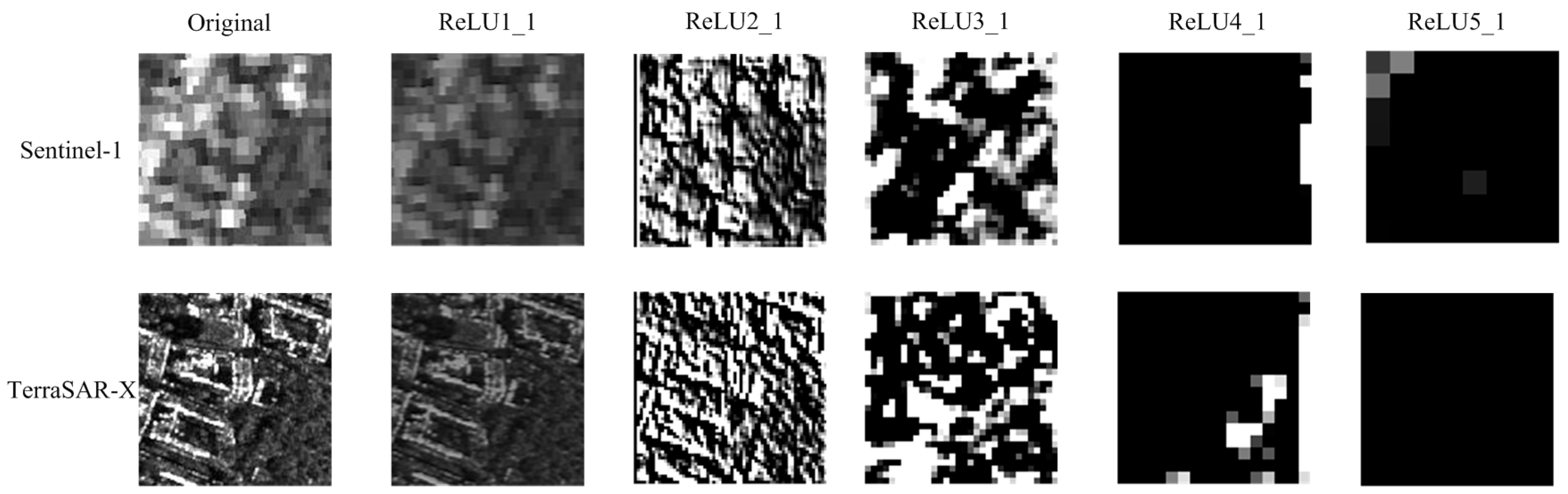
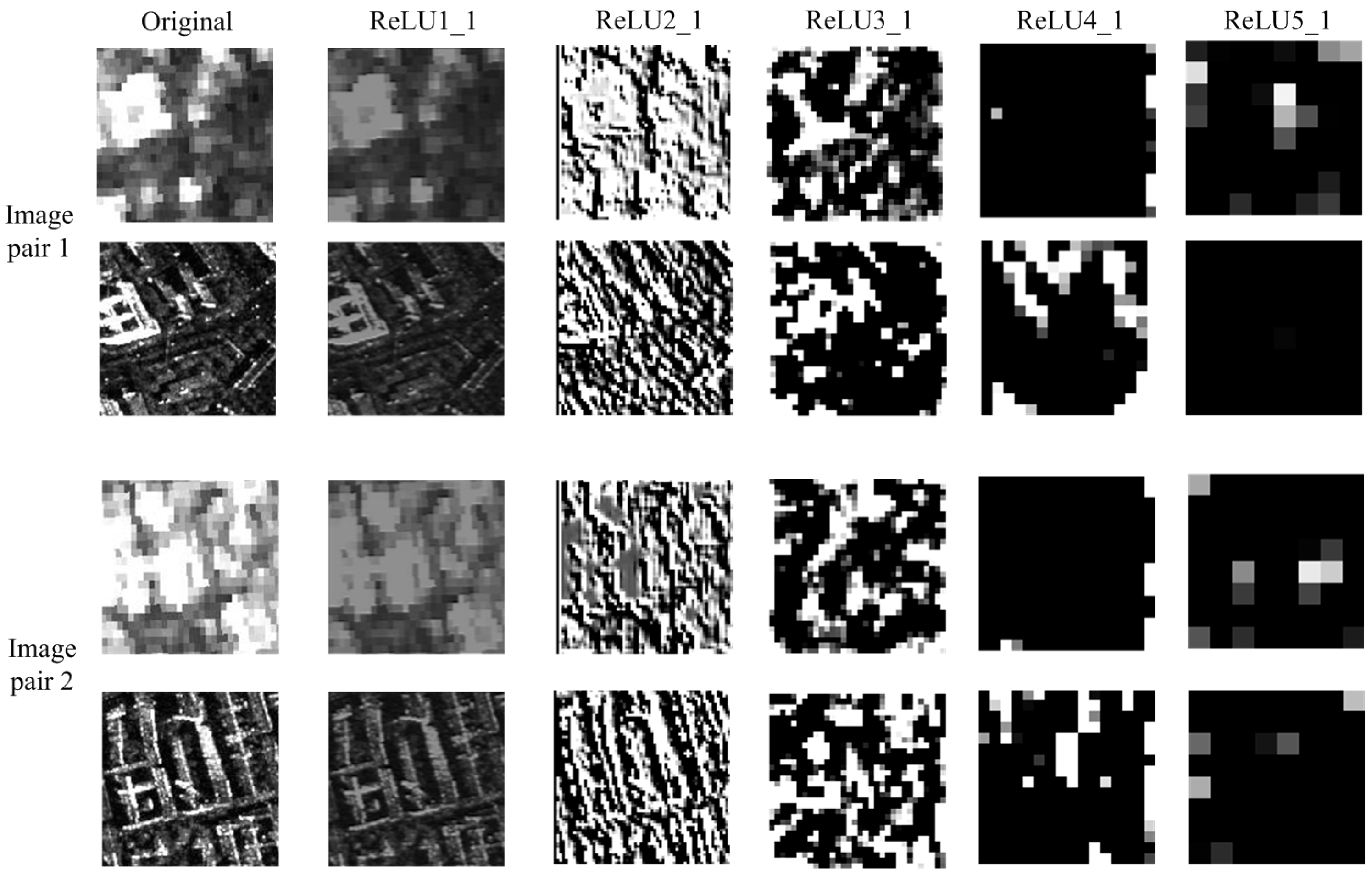
VGG-19 is a key tool to conduct style transfers. It is a pretrained CNN model for large-scale visual recognition developed by Visual Geometry Group at the University of Oxford, which has achieved excellent performances in the ImageNet challenge. Gatys et al. [9] firstly introduced this CNN in their work. Then, the next studies were focused on the utilization of the outcomes of VGG-19. However, VGG-19 has been trained on the ImageNet dataset, which is the collection of optical images. In order to find the capabilities of VGG-19 for SAR images, we first visualized the content of each layer in VGG-19 when the input is a SAR image and then analyzed the meaning of each layer. The input SAR images are in the 8-bit dynamic range without histogram changes for fitting the optical type. There are 19 layers in the VGG-19 network, but the most commonly used layers are the layers after down-sampling, which are called ReLU1_1, ReLU2_1, ReLU3_1, ReLU4_1, and ReLU5_1. The visualization of the middle results in each ReLU layers of VGG-19 is shown in Figure 1.

As can be seen from Figure 1, the images in ReLU 1_1, ReLU 2_1, and ReLU 3_1 layers are similar with the original image, which are called low-level information, while the images in ReLU 4_1 and ReLU5_1 of both two sensors are quite different with the original one, which are called high-level semantic information. According to the conception of deep learning, the higher layers contain higher semantic information [9], which supports the results in Figure 1. Thus, Gatys et al. used the shallow (i.e., lower) layers as the components of texture and took the deep layers as the content information. However, we find that the ReLU5_1 images in both Sentinel-1 and TerraSAR-X are almost featureless. In another paper [27], the authors found that ReLU5_1 has real content for optical images. This may be because this training of VGG-19 is based on optical images. Whatever the cause, we decided to ignore the ReLU5_1 layer in our algorithm to accelerate the computation. This will be discussed in the Experiments section.

3.2. Texture Definition—Gram Matrix

The success of Gatys’ paper is to some extent achieved by the introduction of a Gram matrix. If we regard the pixels of the feature map in each layer as a set of random variables, the Gram matrix is a kind of second-order moment. The Gram matrix in that paper is computed on the selected layers as described in Section 3.1. Assuming $L$ layers are selected, and their corresponding number of feature maps is $N_l$, the Gram matrix of the $l\mathrm{th}$ layer is:

$$G^l=\frac{1}{M_l}\left[\begin{array}{c}{F}_{1:}^l{}^T\\ F_{2:}^l{}^T\\ ⋮\\ F_{N_l:}^l{}^T\end{array}\right]\left[\begin{array}{cccc}{F}_{1:}^l& F_{2:}^l& \cdots & F_{N_l:}^l\end{array}\right],$$

(1)

where $F_{i:}^l$ is the column vector generated from the $i\mathrm{th}$ feature map of layer $l$, and $M_l$ is the size number of each feature map in this layer. An element of the $N^l\times N^l$ Gram matrix is:

$$G_{ij}^l=\frac{1}{M_l}{\displaystyle \sum }_{k=1}^{M_l}{F}_{ik}^l{F}_{jk}^l=\frac{1}{M_l}\langle F_{i:}^l,F_{j:}^l\rangle ,$$

(2)

where $\langle \cdot \rangle$ denotes the inner product. The Gram matrices that we selected are grouped in ${\left\{G^l\right\}}_{l\in {\mathit{L}}_{selected}}$, where ${\mathit{L}}_{selected}$ is the set of the selected layers to define the texture information. Therefore, the definition of the style difference between the two images is:

$${\mathcal{L}}_{style}={\displaystyle \sum }_{l\in {\mathit{L}}_{selected}}{w}_l\Vert {\widehat{G}}^l-G^l{\Vert }_F^2,$$

(3)

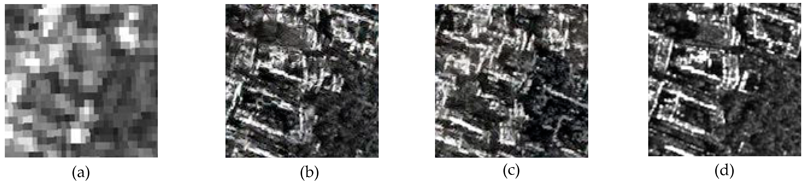
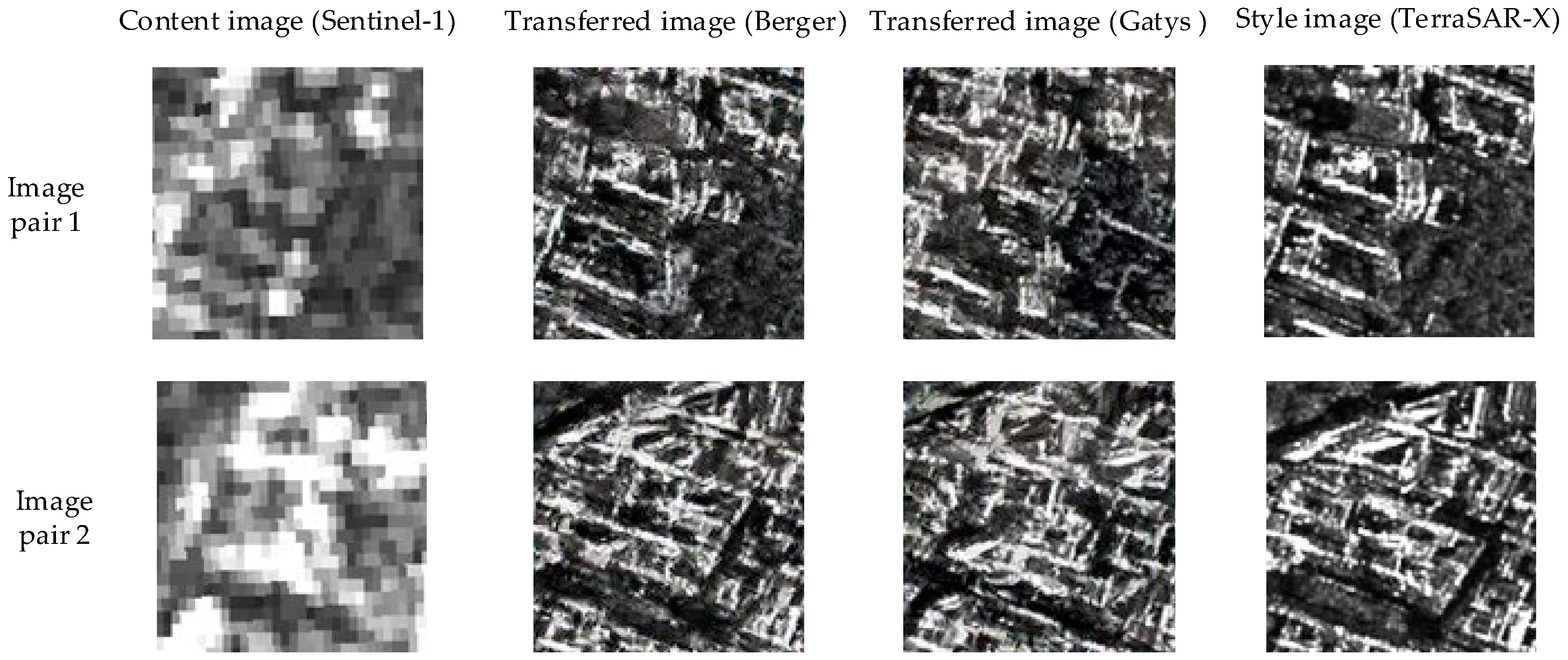
where $w_l$ is a hyper-parameter that defines the weight of the style in the $l\mathrm{th}$ layer, ${\widehat{G}}^l$ is the Gram matrix of the being generated image in the $l\mathrm{th}$ layer, $G^l$ is the corresponding term for the reference image, and $\Vert \cdot \Vert {}_F$ is the Frobenius norm of the matrices. In our case, Gram matrices did not perform well because the style image has more structure information and Figure 2 illustrates this point.

Figure 2b contains many fake targets. For example, there is nothing at the lower right part of Figure 2a,c, but some bright lines, usually from buildings, appear at that same part of Figure 2b. Additionally, contrary to that in Figure 2c, the layout of the buildings in Figure 2b is hard to understand. In our experiment, the SAR data depict an urban area, where most targets are buildings. The city structure is quite different from the design of artistic works, which means the style definition should vary for different applications. Based on these observations, we believe that the format of Gram matrices should be changed to take into account information on spatial arrangement [28], which is important for urban areas. In the following, we discuss this issue in more depth, and propose a solution suitable for our applications.

The arrangement most often indicates the placing of items according to a plan, but without necessarily modifying the items themselves. Thus, an image with arrangement information should contain similar items that placed in different locations. When we tile the images into small pieces (called patches) according to the scheme they belong to, the small pieces should be similar. Their similarity can be determined by the Gram matrix, while the way to tile the image is a part of our approach. The manifestation of most objects of urban areas in remote sensing images is usually rectangular. Thus, the main outline of urban SAR images should be straight lines.

The Spatial Gram method is a good way to represent this arrangement texture, which is defined by the self-similarity matrices themselves and by applying spatial transformations when generating these matrices. A Gram matrix is a measurement of the relationship of two matrices, and the spatial transformation determines which two. G. Berger et al. have proposed a series of CNN-based Spatial Gram matrices to define the texture information. Based on their ideas in [28], we apply a spatial transformation, tiling the feature map horizontally and vertically in different levels to represent the “straight” texture information.

As we have several ways to tile an image, how to compute their Gram matrices for defining the texture of SAR images is still a question, either to add them or to regard them as parallel structures. When the Spatial Gram computation has only one element, it degenerates into the traditional Gram matrix like the one used by Gatys et al. However, when it has too many elements, the ultimate configuration is that all the pixels are in the Gram matrix individually and it has no capability to represent diverse textures. A line, which is the basic unit of our images, can be determined by two parameters. Thus, we use the two orthogonal dimensions ($row$ and $col$) as the two dimensions of the Spatial Gram matrix. Thus, the Spatial Gram matrix we applied in this paper is:

$$S_{spatial}^l=\left(\begin{array}{cccc}{G}_{row,2}^l& G_{row,4}^l& \cdots & G_{row,2^{7-l}}^l\\ G_{col,2}^l& G_{col,4}^l& \cdots & G_{col,2^{7-l}}^l\end{array}\right)$$

(4)

where the type of transformation is related to the size of the feature maps in this layer. ${\mathsf{\Delta }}_l=\left\{2,\dots ,2^{7-l}\right\}$ where the constant 7 is determined by the input size of patches (128 $\times$ 128), and ${\mathit{L}}_{seleted}=\left\{1,2,3\right\}$. $G_{row,\delta }^l$ and $G_{col,\delta }^l$ are two kinds of spatial transformation which relate to the dimensions $row$ and $col$, and the shifted amount $\delta$. Assuming the feature map is $F^l$, and its transformations are $T\left(F^l\right)$, where $T$ denotes the function of spatial transformation. For example, the spatial transformations of feature maps in the row dimension are defined as:

$$T_{row,\delta }\left(F^l\right)=F^l\left(\delta :M,1:N\right), T_{row,-\delta }\left(F^l\right)=F^l\left(1:M-\delta ,1:N\right)$$

(5)

where $M,N$ are the height and width of the feature map $F^l$, respectively. $T_{row,\delta }\left(F^l\right)$ is the transformation on the row dimension. The vectorization of $T_{row,\delta }\left(F^l\right)$ is written as $T_{row,\delta }{\left(F^l\right)}_{:}$, which is the column vector. Having these definitions, $G_{row,\delta }^l$ can be written as:

$$G_{row,\delta }^l=\frac{1}{M_l}\left[\begin{array}{c}{T}_{row,\delta }{\left(F_1^l\right)}_{:}{}^T\\ T_{row,\delta }{\left(F_2^l\right)}_{:}{}^T\\ ⋮\\ T_{row,\delta }{\left(F_{N_l}^l\right)}_{:}{}^T\end{array}\right]\left[\begin{array}{cccc}{T}_{row,-\delta }{\left(F_1^l\right)}_{:}& T_{row,-\delta }{\left(F_2^l\right)}_{:}& \cdots & T_{row,-\delta }{\left(F_{N_l}^l\right)}_{:}\end{array}\right]$$

(6)

where $G_{row,\delta }^l$ can be written in the same way but the spatial transformation takes places in the row direction. Thus, the spatial style loss function is:

$${\mathcal{L}}_{style}={\displaystyle \sum }_{l\in {\mathit{L}}_{selected}}{w}_l\Vert {\widehat{S}}_{spatial}^l-S_{spatial}^l{\Vert }_F^2.$$

(7)

where $S_{spatial}^l$ is the spatial matrices of the target images and ${\widehat{S}}_{spatial}^l$ is for the generated image. The style loss function ${\mathcal{L}}_{style}$ is only dominated by the Spatial Gram matrices; it is not necessary to add the traditional Gram matrices because, when $\delta$ is small, it is almost the same as the traditional one. Figure 3 shows the results applying the new Spatial Gram matrix.

3.3. Conditional Generative Adversarial Networks

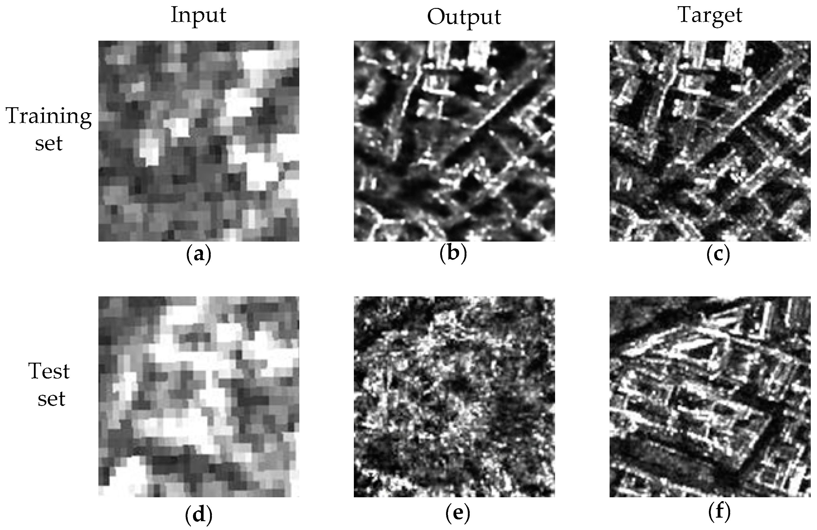
The introduction of GANs is a milestone in deep learning [29]. A conditional GAN makes a general GAN more useful, because the inputs are no longer noise, but signals that we can control. In our case, the conditional inputs are Sentinel-1 images. T The conditional GANs have achieved impressive results on many image processing tasks, such as style transfer [30], super-resolution [31], and other tasks [32,33]. Isola et al. [13] summarized the tasks of image translation as “pix2pix” translations and demonstrated the capabilities of conditional GANs in their paper. Inspired by their works, we modified the “pix2pix” framework by adding new constrains about GANs and specific features of the SAR images translations. When we used the “pix2pix” framework in our application it failed. Figure 4 shows the overfitting of the “pix2pix” conditional GAN because it has good performances on the training set but bad results on the test set. Without any improvement, we could not reach our goals. In the next section, we propose a new method to realize Sentinel-1 to TerraSAR-X image translations.

4. Method

Although conditional GAN is overfitting in our case, it is still a good strategy to complete our task, which is designing a mapping function from Sentinel-1 to TerraSAR-X. In mathematical notation, it is:

$$G:x\to y$$

(8)

where $G$ is the mapping function, $x$ is a Sentinel-1 image, and $y$ is a TerraSAR-X image. Actually, this task can be achieved by designing a neural network and by presetting a loss function, like traditional machine learning. Indeed, this idea has already been accomplished in References [10,11]. However, the preset loss function does not work well in all cases. In GANs, the loss function is not preset, and it can be trained through a network which is called a “Discriminator”. The mapping function $G$ is realized through a “Generator” neural network.

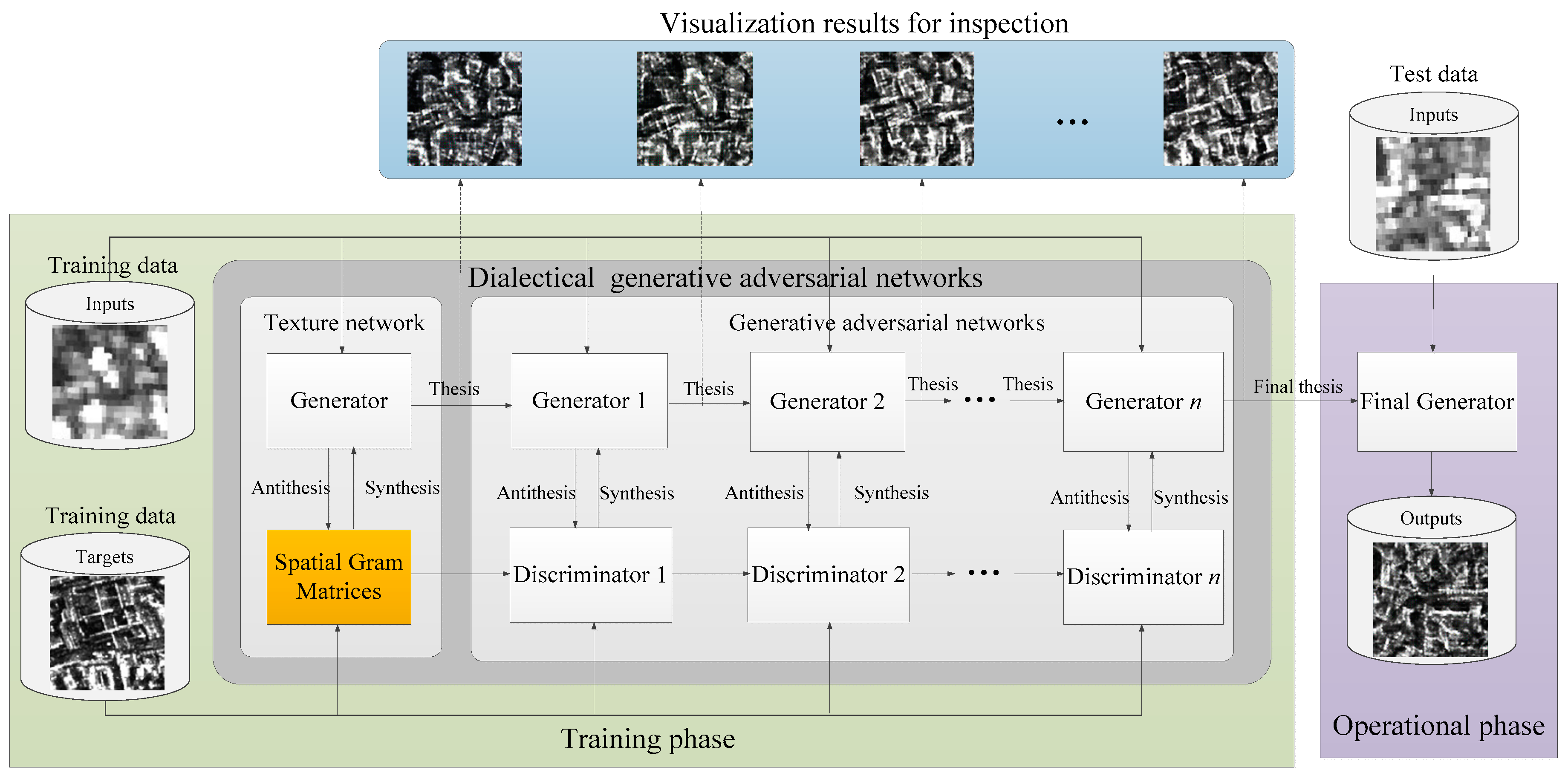
In this paper, we use the concept of dialectics to unify the GANs and traditional neural networks. There is a triad in the system of dialectics, including thesis, antithesis, and synthesis, and they are regarded as a formula for the explanation of change. The formula is summarized as: (1) A beginning proposition, called a thesis; (2) a negation of that thesis, called the antithesis; and (3) a synthesis, whereby the two conflicting ideas are reconciled to form a new proposition [34]. We apply this formula to describe the change of image translation. The “Generator” network is regarded as the thesis and it can inherit the parameters from the previous thesis. In our case, the “Generator” inherits from the texture network. The “Discriminator” network acts as a negation of the “Generator”. The synthesis is based on the law of the Negation of the Negation. Thus, we can generate a new “Generator” through the dialectic. When the new data come, they will enter the next state of changing and developing. The global flowchart of our method is shown in Figure 5. There are two phases, the training phase and the operational phase. The training phase is the processing to generate a final Generator, and the operational phrase applies the final Generator to conduct the image translation task. In the following, we will discuss the “Generator” network, the “Discriminator” network, and the details to train them.

4.1. “Generator” Network—Thesis

The purpose of the Generator is to generate an image $G\left(x\right)$ that has the content of image $x$ and the style of image $y$. Thus, the loss function has two parts, the content loss and the style loss, which is defined as:

$$\begin{array}{cc}\hfill {\mathcal{L}}_{Generator}& ={\mathcal{L}}_{content}+\lambda {\mathcal{L}}_{style}\hfill \\ \hfill & ={\displaystyle {\displaystyle \sum }_{l\in {\mathit{L}}_{content}}}\Vert F^l\left(G\left(x\right)\right)-F^l\left(x\right){\Vert }_F^2+\lambda {\displaystyle \sum }_{l\in {\mathit{L}}_{style}}{w}_l\Vert S_{spatial}^l\left(G\left(x\right)\right)-S_{spatial}^l\left(y\right){\Vert }_F^2,\hfill \end{array}$$

(9)

where $\lambda$ is a regularization parameter, $F^l(\cdot )$ are the feature maps of the $l\mathrm{th}$ layer of an image, and $S_{spatial}^l(\cdot )$ are the Spatial Gram matrices that were defined in Section 3.2. According to the discussion in Section 3.1, there is little information in “ReLU5_1” layer, which makes it a burden for computation because of its depth. Therefore, we chose “ReLU4_1” as the content layer, and “ReLU1_1”, “ReLU2_1”, and ”ReLU3_1”as the style layers. Consequently, ${\mathit{L}}_{content}=\left\{4\right\}, \mathrm{and} {\mathit{L}}_{style}=\left\{1,2,3\right\}$.

$G$ can be any kind of function. For example, it can be as simple as a linear function or as complex as a multiple composition of nonlinear functions. As a powerful tool to approximate functions [35,36], we chose to use deep neural network as generators in this paper. The input and the target images, $x$ and $y$, are from different SAR sensors, but they are observing the same test site. The properties of SAR systems result in their own characteristics of image representation, such as final resolution, polarization response, and the dynamic ranges. However, the same observed area makes them share identical compounds. Regardless of the changes in time, $x$ and $y$ are generated from identical objects. For the analysis of our input and target images, there are plenty of network structures that solve this problem.

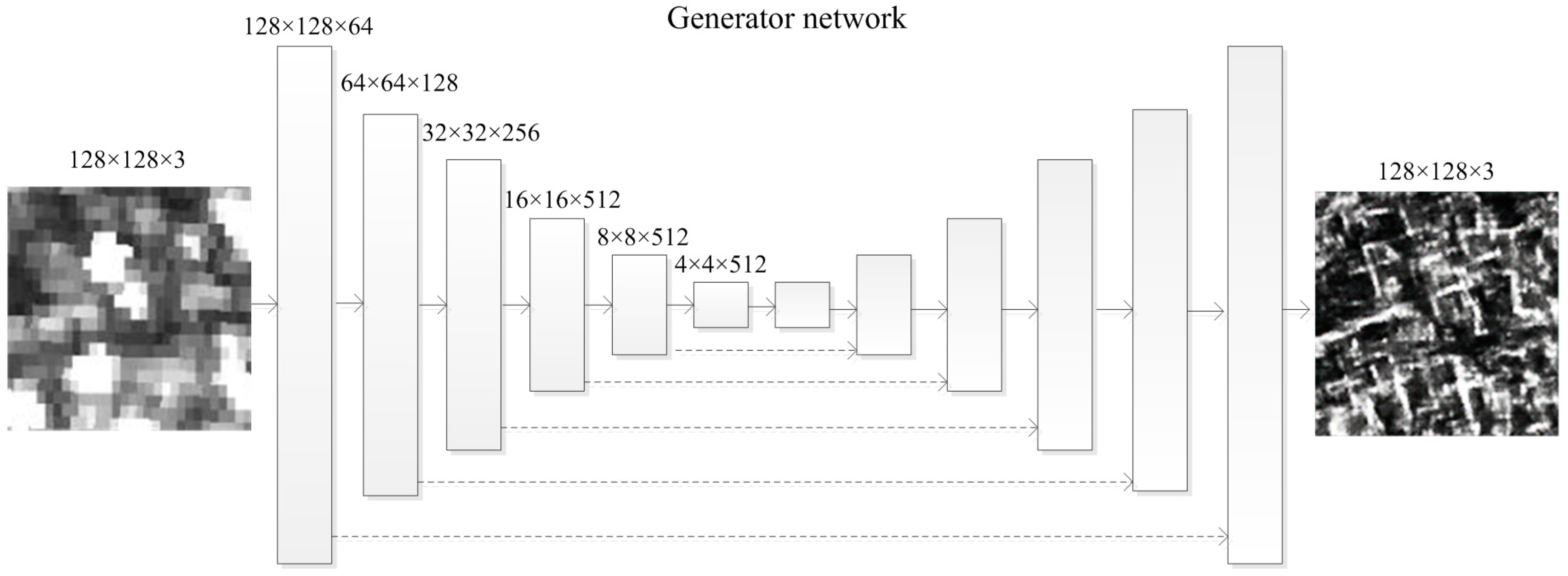
Previous related works [32,37] have used an encoder–decoder network [38], where the input image is compressed in down-sampled layers and then be expanded again in up-sampled layers, where the process is reversed. The main problem with this structure is whether the information is preserved in the down-sampled layers. Based on the discussion in Reference [13], we chose the “U-Net” network to execute our tasks. The “U-Net” is very well known for its skip connections, which are a way to protect the information from loss during transport in neural networks. According to the anaylsis of our SAR images in the VGG-19 network, we set the “U-Net” to 12 layers. The structure of the network we used is shown in Figure 6.

Although the network in Figure 5 has too many elements and is hard to be trained, we think it is necessary to use a deep network, because the architecture of a network can affect its expressiveness of complex functions. Maybe there will be more efficient methods to approximate the mapping function, but this is not the topic of this paper. Our goal here is to find a powerful tool to describe the mapping from Sentinel-1 to TerraSAR-X, and the solution is a deep neural network.

4.2. “Discriminator” Network—Antithesis

A deep neural network is a suitable solution, but on the other hand, it can also easily generate nontarget results. Based on the concept of dialectics, when the appearance is not fit for the conception, it is needed to deny the existence of this thing. In this case, it is the negation of the generated images. In other words, we need a loss function yielding a small value when the output equals the target, while yielding a high value when the two things are different. Usually, the loss function is predefined. For example, the most common loss function, Mean Squared Error (MSE), is a preinstalled function which is defined as:

$$MSE=\frac{1}{N}{\displaystyle \sum }_{i=1}^N{\left(Y^i-{\widehat{Y}}^i\right)}^2,$$

(10)

where $\widehat{Y}$ is the generated vector of $Y$ whose elements are $Y^i$. When computing the MSE function, it outputs a scalar value to describe the similarity between the input and the target. However, it is predefined, and the only freedom is the input data. How it relates to the negation of the generated images is still a question. There are three steps to solve the problem. First, the loss function should criticize the existence of $\widehat{Y}$, so it has a term $-\widehat{Y}$. Second, it should approve the subsistence of $Y$, the target; thus, the term $Y$ shall appear. Third, the square operator makes sure the function is a kind of distance. Through these three steps, the MSE has accomplished the negation of the generated vectors or images. When the generated image differs from the target image, the distance is large. When the generated image is the target image itself, their distance shall be zero. By contrast, a large distance shall be generated when the input is markedly different from the target, representing a better negation.

It is reasonable to assume that the loss function is a kind of distance function, because the distance space is a weak one compared with the norm space and the inner product space. For instance, the loss function in Equation (9) is another kind of distance compared with the MSE that directly computes pixel values. However, it is hard to find a unique common distance, because our tasks differ, while the distance remains invariant. Using a neural network scheme to train a distance is a good choice. Fortunately, the appearance of GANs has provided us with a solution to find the proper distances. In GAN systems, the negation of generated images is processed in the loss function of the “Discriminator”. The Discriminator is a mapping function, which is in the format of the neural network to describe the existence of the input image. However, little discussion has been made on the Discriminator properties. In this paper, we try to use the theory of metric spaces to discuss this question.

Assuming that the distance in the image domain $M_1$ is $d_1(\cdot )$ and the distance in the Discriminator domain $M_2$ is $d_2(\cdot )$, the Discriminator is the map $D:M_1\to M_2$ [39]. The distance of the conditional case, which is also the $\mathrm{contradiction}$ between the two images, can be defined as:

$${\mathcal{L}}_{\mathrm{contradiction}}=d_2\left(D\left(y|x\right),D\left(G\left(x\right)|x\right)\right)$$

(11)

where $D\left(\cdot |x\right)$ is the Discriminator of an image under the condition that the input is $x$. If $D(\cdot )$ is a function to map the image to itself, and $d_2(\cdot )$ is the Frobenius norm, the contradiction becomes:

$${\mathcal{L}}_{\mathrm{contradiction}}=\Vert y-G{\left(x\right)\Vert }_F$$

(12)

which is the $L_1$ norm that usually acts as a loss function in machine learning. This is one case of a determined map. As for a training map function, the most important thing is to design its format. If we still set $d_2(\cdot )$ as the Frobenius norm, the distance of the Discriminator becomes:

$${\mathcal{L}}_{\mathrm{contradiction}}=\Vert D\left(y|x\right)-D{\left(G\left(x\right)|x\right)\Vert }_F$$

(13)

When the Discriminator is a predefined network, such as the Spatial Gram matrix, we conclude that the loss function in Equation (9) can be regarded as a specific case of Equation (13).

If the range of $d_2(\cdot )$ is $\left[0,1\right]$, it is considered that the output is the possibility of being real(or fake). Now, there are many concepts to reunite the formats of different loss functions. In $f$-GAN [40], the authors unified the loss function of many GAN models as a version of $f$-divergence, which is a measurement for the similarity of two distributions. However, the drawback of divergences is that they don’t satisfy triangle inequality and symmetry, which are requirements of distance functions [41]. Thus, the $f$-GAN is not the perfect GAN model. The modifications of GAN models are mostly based on the loss function. In LSGAN (Least Squares GAN) [42], the least squares method is used to measure the output of the Discriminator. In this method, the generated images are in an inner product space, which is also a metric space. Therefore, we infer that the contradiction between the real image and the generated image should be contained in a function that can define the distance of some metric space, and map $D$ should be constrained. One constraint of $D$ is that the range of $D$ should be bounded, because the infinite number is unacceptable for computers. Second, $D$ should be continuous, even uniformly continuous, because the gradient descent algorithms may fail when the loss function is not continuous. In WGAN, the Wasserstein distance is used, where the Lipschitz-continuous map ensures the property of uniform continuity. In this paper, we focus on the WGAN framework.

When $d_2(\cdot )$ is the Wasserstein distance [43], the loss function of the Discriminator becomes:

$${\mathcal{L}}_{\mathrm{discriminator}}=W\left(D\left(y|x\right),D\left(G\left(x\right)|x\right)\right)$$

(14)

where $W(\cdot )$ is the Wasserstein distance function, which behaves better than the $f-divergence$ being used in traditional GANs. The realization of the Wasserstein distance enforces a Lipschitz constraint on the Discriminator. In the Wasserstein Generative Adversarial Network—Gradient Penalty (WGAN-GP) framework [44], the Lipschitz constraint is realized by enforcing a soft version of the constraint with a penalty on the gradient norm for random samples $\widehat{x}~{\mathbb{P}}_{\widehat{x}}$, where $\widehat{x}=ϵy+\left(1-ϵ\right)G\left(x\right)$. Based on the conclusions in WGAN [44], the maximum of the Wasserstein distance between ${\mathbb{P}}_{r,y|x}$ and ${\mathbb{P}}_{g,x}$ becomes:

$$D^{*}=\underset{D}{\max }\left({\mathcal{L}}_{\mathrm{discriminator}}\right)=\underset{D}{\min }\left(\begin{array}{c}\underset{G\left(x\right)~{\mathbb{P}}_{g,x},x~{\mathbb{P}}_{r,x}}{\mathbb{E}}\left[D\left(G\left(x\right)|x\right)\right]-\underset{y~{\mathbb{P}}_{r,y},x~{\mathbb{P}}_{r,x},}{\mathbb{E}}\left[D\left(y|x\right)\right]\\ +{\lambda }_{gp}\underset{\widehat{x}~{\mathbb{P}}_{\widehat{x}}}{\mathbb{E}}[{\left({\Vert {\nabla }_{\widehat{x}}D\left(\widehat{x}|x\right)\Vert }_2-1\right)}^2]\end{array}\right)$$

(15)

where $D^{*}$ is the best Discriminator, $\mathbb{E}(\cdot )$ is the expectation operator, ${\mathbb{P}}_{r,y|x}$ is the distribution of given real images, ${\mathbb{P}}_{g,x}$ is the distribution of generated images, and ${\nabla }_{\widehat{x}}D\left(\widehat{x}|x\right)$ is the gradient of the Discriminator $D\left(\cdot |\cdot \right)$. When adding the penalty of the distance between the normal of ${\nabla }_{\widehat{x}}D\left(\widehat{x}|x\right)$ and 1 in the loss function, the Discriminator is forced to become a $1-Lipschitz$ function. ${\lambda }_{gp}$ is usually set to 10 according to the experiments conducted in Reference [44]. Intuitively, the removal of the absolute operator ensures the continuity of the derivation of the loss function at the origin. The $1-Lipschitz$ constraint limits the normal of the derivation from growing too large, which is a way to increase the distance, but not the way we want.

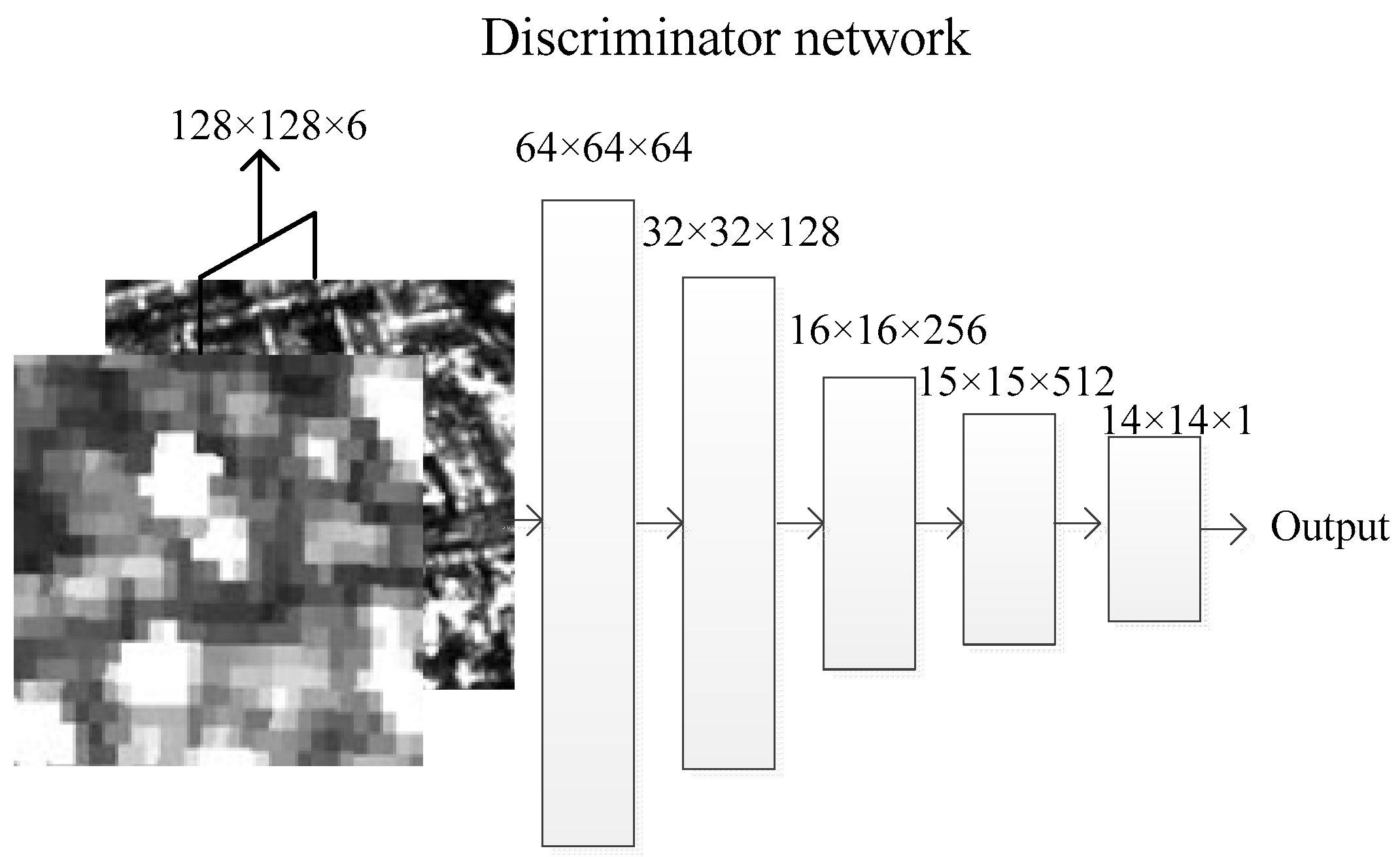
Once the loss function is determined, the next step is to design the architecture of $D\left(\cdot |x\right)$ that can be easily trained. Considering the ready-made function already discussed in the previous section, the loss function of style defined by Gram matrices is a good choice, because it can be regarded as processing on a Markov random field [13,29]. The “pix2pix” summarized it as the “PatchGAN” whose input is the combination of $x$ and $y$. The architecture of the Discriminator is shown in Figure 7.

4.3. Dialectical Generative Adversarial Networ—Synthesis

According to the dialectic, the third step is the negation of the negation. The negation of the generated image is described by the loss function of the Discriminator. Thus, the negation of the negation should be the negation of the loss function of the Discriminator. The negation is trying to make the distance defined by the Discriminator become larger, while the negation of the negation should make the distance smaller. In our framework, the negation is defined by Equation (15). Thus, the negation of the negation can be realized by maximizing it. Therefore, the maximization of the loss function in Equation (15) is the negation of the negation. At the last step of the dialectic, the negation of the negation should be combined with the thesis to form a synthesis.

The thesis can be regarded as a synthesis from the former dialectics. For example, the “pix2pix” used the $L_1$ norm as their thesis, and the SRGAN (Super Resolution GAN) used the Gram matrices on the 5th layer of the VGG-19 network as their thesis. These initial loss functions are distance functions and contain the negation of the generated images. In this paper, we start from the thesis defined by a Spatial Gram matrix. In other words, we set the initial loss function as defined in Equation (9). The negation of the negation is the maximization of Equation (15). Therefore, the synthesis of our “Dialectical GAN” is the combination of Equations (9) and (15). Reducing the terms that are independent of “Generator” networks, the loss function of the “Dialectical GAN” becomes:

$$\begin{array}{cc}\hfill {\mathcal{L}}_{Generator}^{GAN}& ={\mathcal{L}}_{Generator}-{\lambda }_{GAN}{\mathcal{L}}_{critical}\hfill \\ \hfill & ={\mathcal{L}}_{content}+\lambda {\mathcal{L}}_{style}-{\lambda }_{GAN}\underset{G\left(x\right)~{\mathbb{P}}_{g,x},x~{\mathbb{P}}_{r,x}}{\mathbb{E}}\left[D\left(G\left(x\right)|x\right)\right]\hfill \end{array}$$

(16)

where ${\mathcal{L}}_{critical}$ is the negation of the generated image. To optimize this new loss function, we need four steps: Set up the Generator, update the Discriminator, update the Generator, and iterate.

• Step 1, having a Generator $G(\cdot )$ and an input image $x$, use them to generate $G\left(x\right)$, and then run the Discriminator $D\left(\cdot |\cdot \right)$.
• Step 2, use gradient descent methods to update $D\left(\cdot |\cdot \right)$, following (15).
• Step 3, use gradient descent methods to update $G(\cdot )$, following (16).
• Step 4, repeat Step 1 and Step 3 until the stopping condition is met.

Then, the training of the Dialectical GAN is completed. Every loop can be considered as a realization of the dialectics. The basic framework is based on the WGAN-GP. As for the mathematical analysis of the GANs and deep learnings, please refer to References [45,46,47]. Although Deep Learning still looks like a “black box”, we tried to provide a logical analysis of it and attempted to achieve “real” artificial intelligence with the capabilities of dialectics.

5. Experiments

Based on the method proposed in Section 4, the GAN network used in this paper has two neural networks, Generator and Discriminator. The Generator is a “U-Net” with 6 layers, and the Discriminator is a “PatchGAN” convolutional neural network with 4 layers. In total, we had 1860 image pair-patches in the training data set and 224 image pair-patches in the test data set, which were preprocessed according to the methods in Section 2. With these data sets, the training of 200 epoch took 3000 min on a laptop with Intel Xeon CPU E3, an NVidia Q2000M GPU, and 64 GB of memory. We conducted three experiments with respect to the following networks further presented below.

5.1. SAR Images in VGG-19 Networks

The VGG-19 has an essential role in this paper because its layers are the components of the texture information determined by a Gram matrix. Additionally, the selection of the content layer is a new problem for SAR images. First, we compared the differences between Sentinel-1 and TerraSAR-X images in each layer. The two image patch-pairs are the inputs in the VGG-19 networks and their intermediate results are shown in Figure 8.

Visually, the images of the ReLU4_1 layer have common parts. However, this is not enough, and we decided to introduce the MSE and the Structural Similarity Index (SSIM) [48] in order to compare the image in different layers. The MSE is defined as:

$$MS{E}^l=\frac{1}{{\left(M^l\right)}^2{N}^l}{\displaystyle \sum }_{k=0}^{N^l-1}{\displaystyle \sum }_{i=0}^{M^l-1}{\displaystyle \sum }_{j=0}^{M^l-1}{\left[x_k^l\left(i,j\right)-y_k^l\left(i,j\right)\right]}^2,$$

(17)

where $M^l$ is the size of the feature maps in $l\mathrm{th}$ layer, $N^l$ is the number of the feature maps in $l\mathrm{th}$ layer, $x_k^l\left(i,j\right)$ is the pixel value of $\left(i,j\right)$ in the $k\mathrm{th}$ feature map of the $l\mathrm{th}$ layer of a Sentinel-1 image, and $y_k^l\left(i,j\right)$ is the counterpart of a TerraSAR-X image. In order to overcome the drawbacks of the MSE, we applied the SSIM, whose definition is:

$$SSIM\left(x,y\right)=\frac{\left(2{\mu }_x{\mu }_y+c_1\right)\left(2{\sigma }_{xy}+c_2\right)}{\left({\mu }_x^2+{\mu }_y^2+c_1\right)\left({\sigma }_x^2+{\sigma }_y^2+c_2\right)},$$

(18)

where ${\mu }_x$ and ${\sigma }_x$ are the mean value and the standard deviation of image $x$; the same to applies to $y$. $c_1$ and $c_2$ are two constants related with the dynamic range of the pixel values. For more details, we refer the reader to Reference [48]. The SSIM values range between −1 and 1, where 1 indicates perfect similarity. The evaluation results under two indicators are shown in

Table 2. Evaluation results with the Mean Squared Error (MSE) and Structural Similarity Index (SSIM).

Layers	MSE	SSIM
ReLU1_1	0.1616	0.4269
ReLU2_1	0.5553	0.0566
ReLU3_1	0.5786	0.2115
ReLU4_1	0.3803	0.7515
ReLU5_1	0.2273	0.7637

.

Although ReLU5_1 has the best performance with two indicators, we still ignore this layer, due to the poor diversity in this layer. Excluding ReLU5_1, the ReLU4_1 layer gives us the best result. There will not be too many differences between ReLU5_1 and ReLU4_1 (Figure 9). Moreover, training processing with ReLU4_1 will be faster than that with ReLU5_1. When choosing ReLU5_1, the speed is 2.1 images/s, while the speed is 2.3 images/s for ReLU4_1. Considering the large scale of the training phase and the real effect, ReLU4_1 is chosen as the content layer, and the first three layers are used to define texture information.

5.2. Gram Martrices vs. Spatial Gram Martrices

A Spatial Gram matrix is an extension of a Gram matrix, which is used to describe texture information and is good at representing arrangement information. In Section 3.2, we have shown the visual difference between two style definitions. In this experiment, we used the quantity indicators to evaluate the two methods. Two image patch-pairs were chosen to conduct the comparison, whose results are shown in Figure 10. In order to evaluate the image quality of the SAR images, we introduce the equivalent numbers of looks (ENL), which act as a contrast factor to represent the image resolutions approximately. Although the ENL is an indicator for speckle, it has a negative correlation with the image resolution. Here, the ENL is computed in on the whole patch. Looks are the sub-images formed during SAR processing where the image speckle variance is reduced through multilook processing. However, a degradation of the geometric resolution occurs due to the reduction of the processed bandwidth [49]. Thus, a higher ENL value indicates that the image is smooth, while a lower value means that the image is in high resolution [50]. For our case, we need high-resolution images and, as a result, the lower their ENL value, the better. The definition of ENL is:

$$ENL=\frac{{\mu }^2}{{\sigma }^2}$$

(19)

where $\mu$ is the mean value of the image patch and $\sigma$ is its standard deviation.

As can be seen from Figure 10 and

Table 3. Evaluation of two methods for both image pairs 1 and 2.

Image Pairs	Methods	MSE	SSIM	ENL
1	Gatys et al. Gram	0.3182	0.0925	1.8286
	Spatial Gram	0.2762	0.1888	2.0951
2	Gatys et al. Gram	0.3795	0.0569	2.0389
	Spatial Gram	0.3642	0.0700	1.9055

, the Spatial Gram method performs better than Gatys et al.’s method, both visually and according to evaluation indicators. However, the ENL of image pair 1 indicates that Gatys et al.’s method is better. To solve this problem, we need more experiments. Because the traditional generative model regards every pixel as a random pixel and ignores the relationships among neighboring pixels, its computing efficiency is limited. Nevertheless, a Spatial Gram matrix is a good tool to determine the image style for our cases. In the next subsection, we have abandoned Gatys et al.’s method and replaced it with a “U-net” network to generate the enhanced images. This method is called “Texture network”.

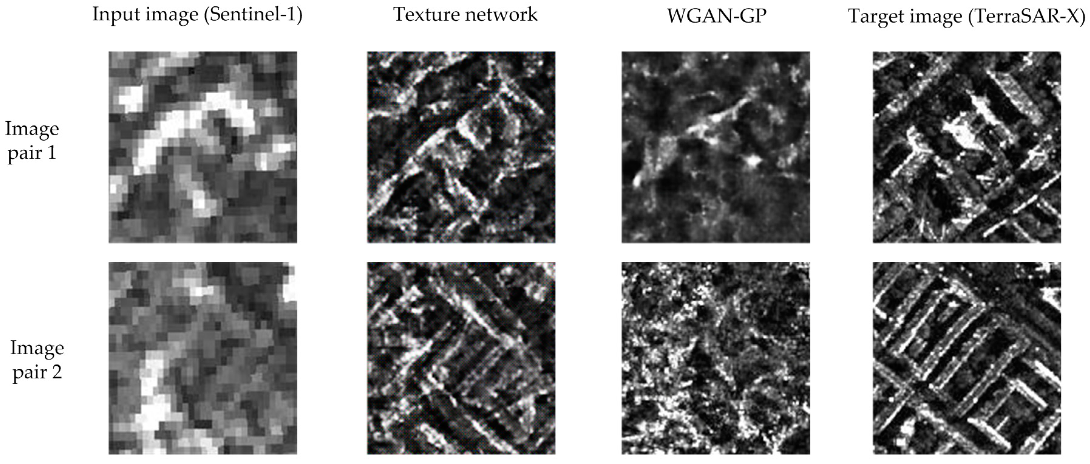
5.3. Spatial Gram Matrices vs. Traditional GANs

The texture network moves the computational burden to a learning stage and no longer needs the style images as an aide to produce an image, because the style information is already mapped in the network through the learning steps. Although the feed-forward network supersedes the solution of random matrices, the loss function is still the same. According to the above experiments, the Spatial Gram matrix is the one we chosen.

In contrast to the determinate one, other researchers found that the loss function can also be learned, though the Spatial Gram matrix is also learned from the VGG-19 network. Nonetheless, the learning of the loss function enables the definition of image style to become more optional. We use the WGAN-GP framework to represent this kind of idea, which is the most stable one among the GAN family. The results of the texture network and the WGAN-GP are compared in Figure 11, and the evaluation results are listed in

Table 4. Evaluation of Texture network and WGAN-GP in both image pair 1 and 2.

Image Pairs	Methods	MSE	SSIM	ENL
1	Texture network	0.3265	0.0614	1.3932
	WGAN-GP	0.2464	0.1993	2.8725
2	Texture network	0.3396	0.0766	1.6269
	WGAN-GP	0.2515	0.2058	3.5205
Test set	Texture network	0.3544	0.0596	1.7005
	WGAN-GP	0.2632	0.2117	3.3299

. The test set components in Table 4 are the average performances of images in the whole test set. Especially, the SSIM is quite low in both methods because the input image and the target image are not totally from the same target as the traditional super-resolution tasks. Since Sentinel-1 and TerraSAR-X are with different radar parameters, it is reasonable that the two images have different content. We need to generate an image with the content of Sentinel-1 but its style should be that of TerraSAR-X., Therefore, the original difference reflects on the final performance as a result that SSIM becomes low in Table 4.

The texture network and the WGAN-GP are fast ways to conduct style transfer. According to the values in Table 4, we concluded that the WGAN-GP has a better performance than the texture network method with the given indicators. However, the WGAN-GP is not able to preserve the content information of Sentinel-1 and its output images are muddled without obvious structures, like the texture network. Although the texture network has no good performance in the evaluation system, it has a preferable visual effect in contrast to the WGAN-GP. How to balance the indicator values and the visual performance is a crucial problem. The texture information is defined by the VGG-19 network, which has been trained by optical images. Thus, we have grounds to believe that there is texture information that cannot be fully described by Spatial Gram matrices. In the following experiment, we will compare the texture network with the proposed Dialectical GAN.

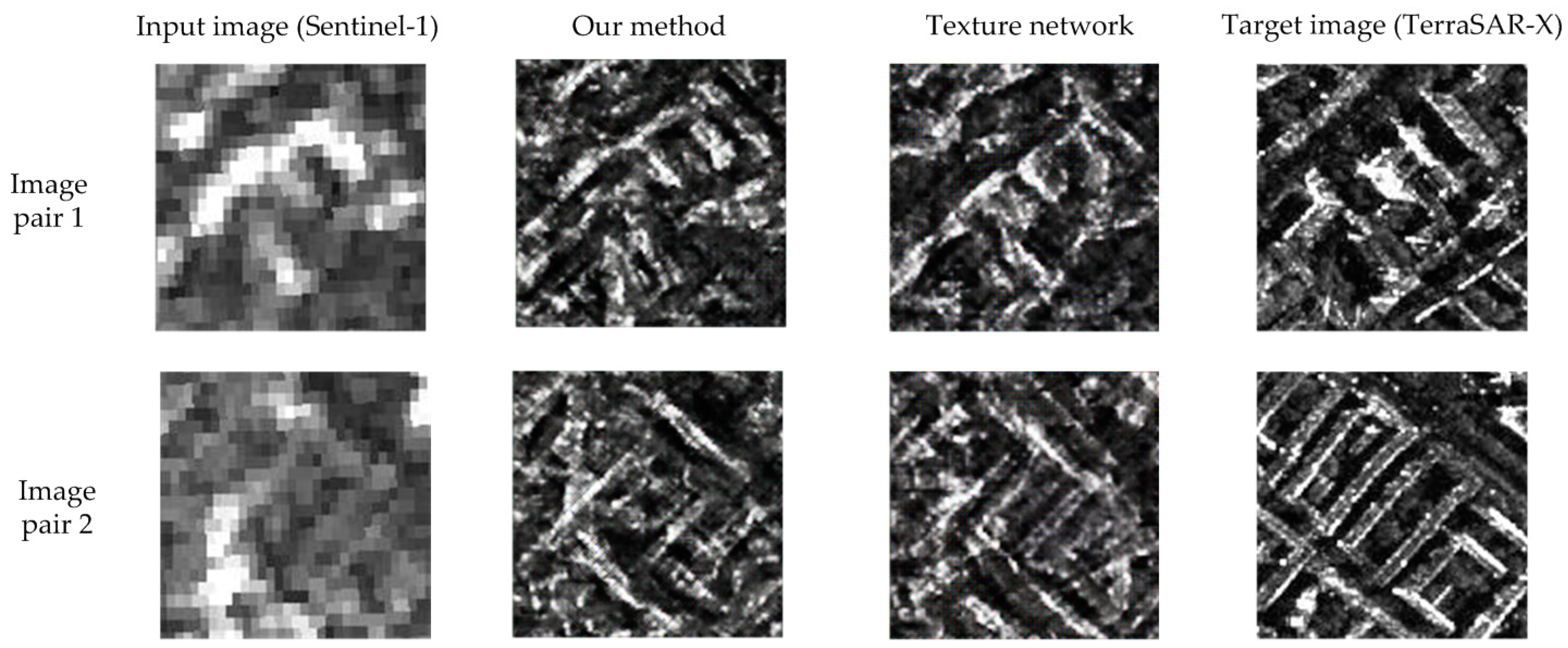
5.4. The Dialectical GAN vs. Spatial Gram Matrices

The texture network defined the texture information in a determinate way, while the WGAN-GP uses a flexible method to describe the difference between generative images and target images. In this paper, we proposed a new method that combines a determinate way and a flexible way to enhance the generative images, and we called it “Dialectical GAN” because the idea is enlightened by the dialectical logic. The Dialectical-GAN initializes its loss function with the Spatial Gram matrix that was found as a good way to describe the texture information of the urban area and the content loss defined by the ReLU4_1 layer of the VGG-19 network. Through the training of the Dialectical GAN, new texture information can be learned and represented in the “Discriminator” network. The comparison between a “Dialectical GAN” and the texture network with a Spatial Gram loss function are shown in Figure 12 and

Table 5. Evaluation of Texture network and Dialectical GAN for both image pairs 1 and 2.

Image Pairs	Methods	MSE	SSIM	ENL
1	Texture network	0.3264	0.0614	1.3933
	Dialectical GAN	0.3291	0.0884	1.5885
2	Texture network	0.3396	0.0766	1.6270
	Dialectical GAN	0.3310	0.0505	1.8147
Test set	Texture network	0.3544	0.0596	1.7005
	Dialectical GAN	0.3383	0.0769	1.8804
Original data	Sentinel-1	0.3515	0.1262	5.1991
	TerraSAR-X	-	-	1.6621

.

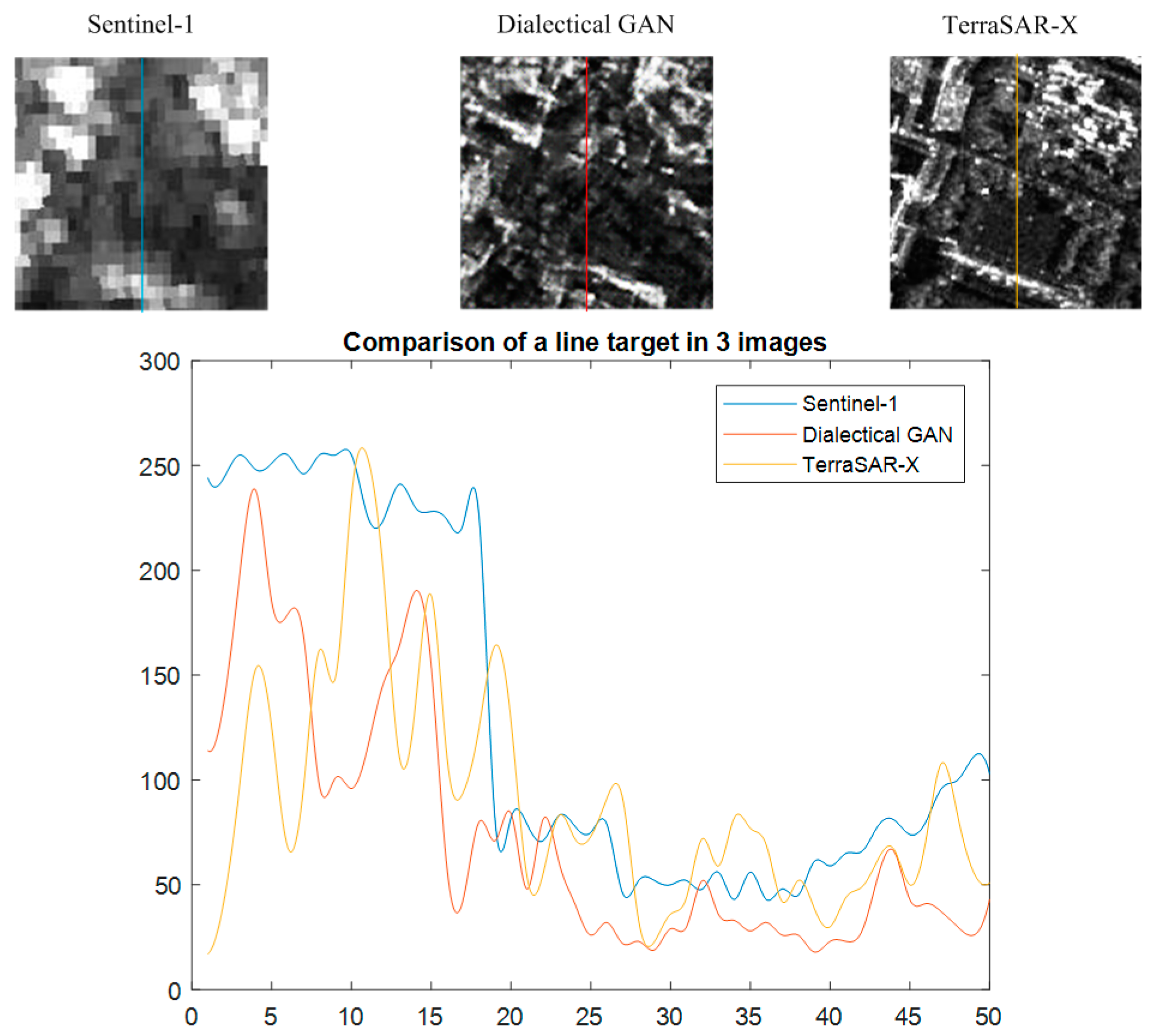
Both visual performance (Figure 12) and the indicator analysis (Table 5) proved that our method is better than the texture network. The original data are also compared in Table 5. The above analysis is all at image level. With respect to the signal level, we can evaluate some typical targets in these images. In Figure 13, we have chosen a line-like target to demonstrate the high-resolution result of our method. At the bottom of this image patch, there is a small line-like target. We have drawn three signal profiles along the middle line direction in Figure 13, where the resolution of the Dialectical GAN is much higher than that of Sentinel-1.

However, these experiments all remained limited to the patch level, and the figures for a whole scene have not yet been considered. Therefore, we show the entire image composited with every patch to check the overall performance and to estimate the relationship between neighboring patches.

5.5. Overall Visual Perfomance

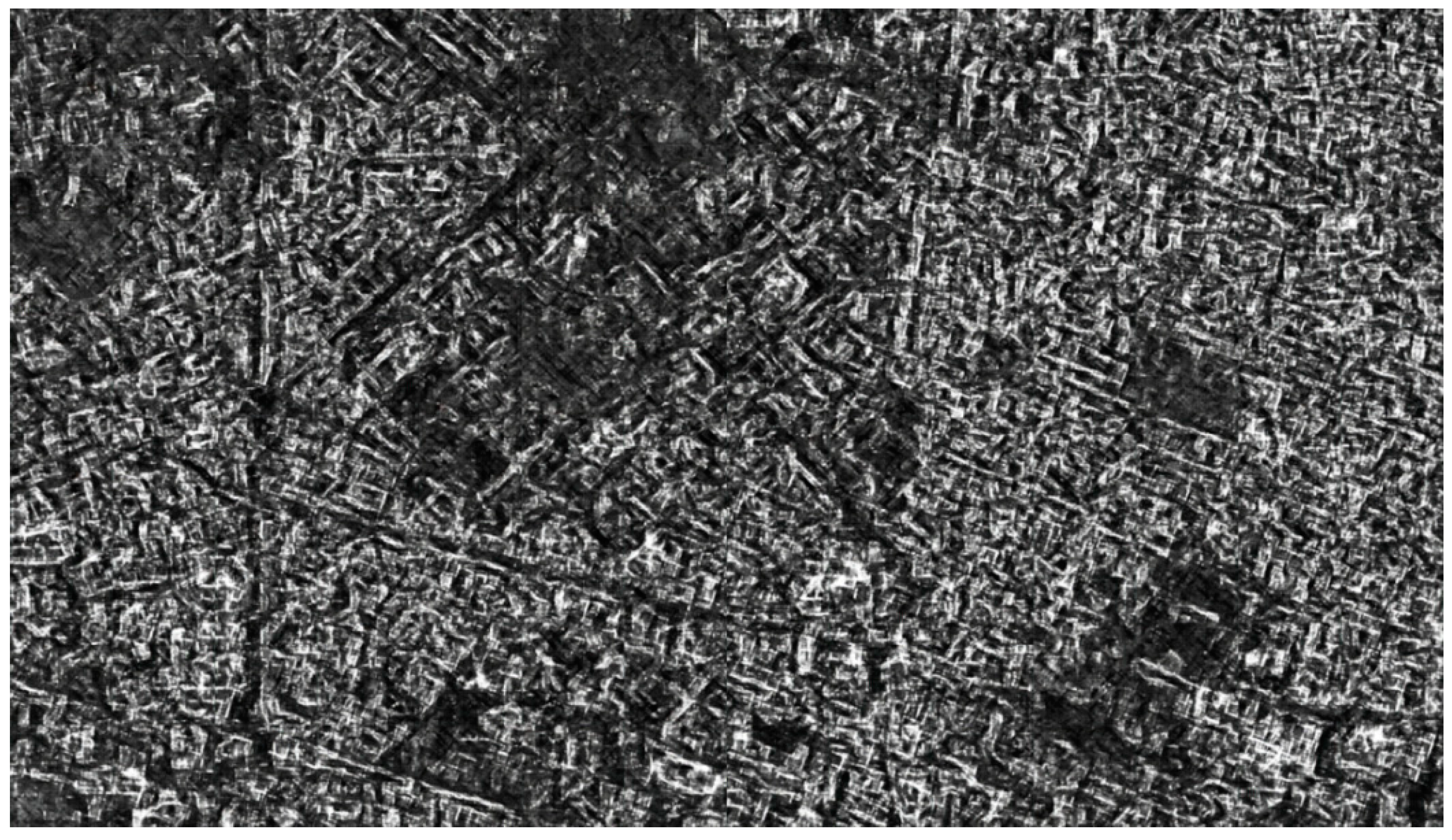
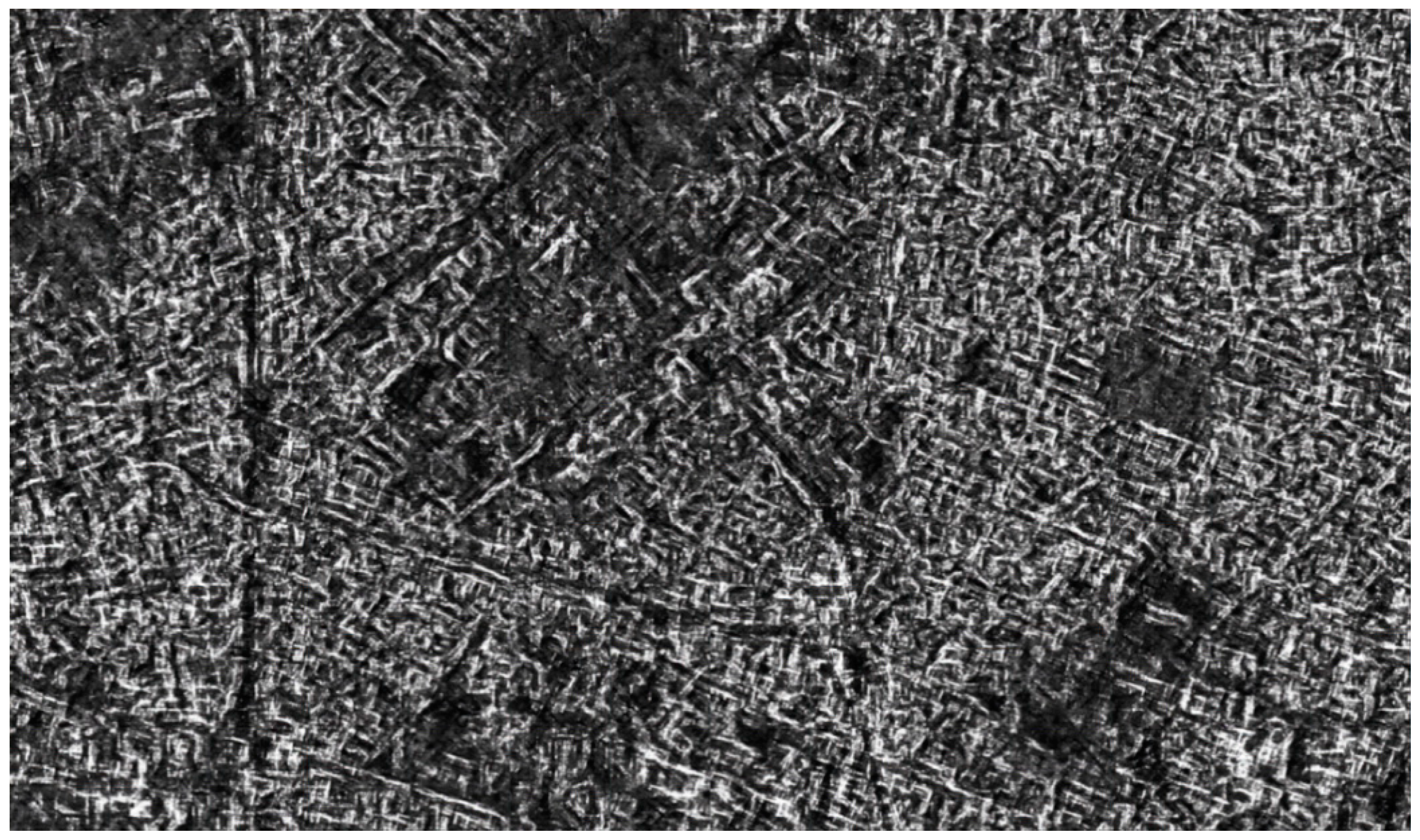
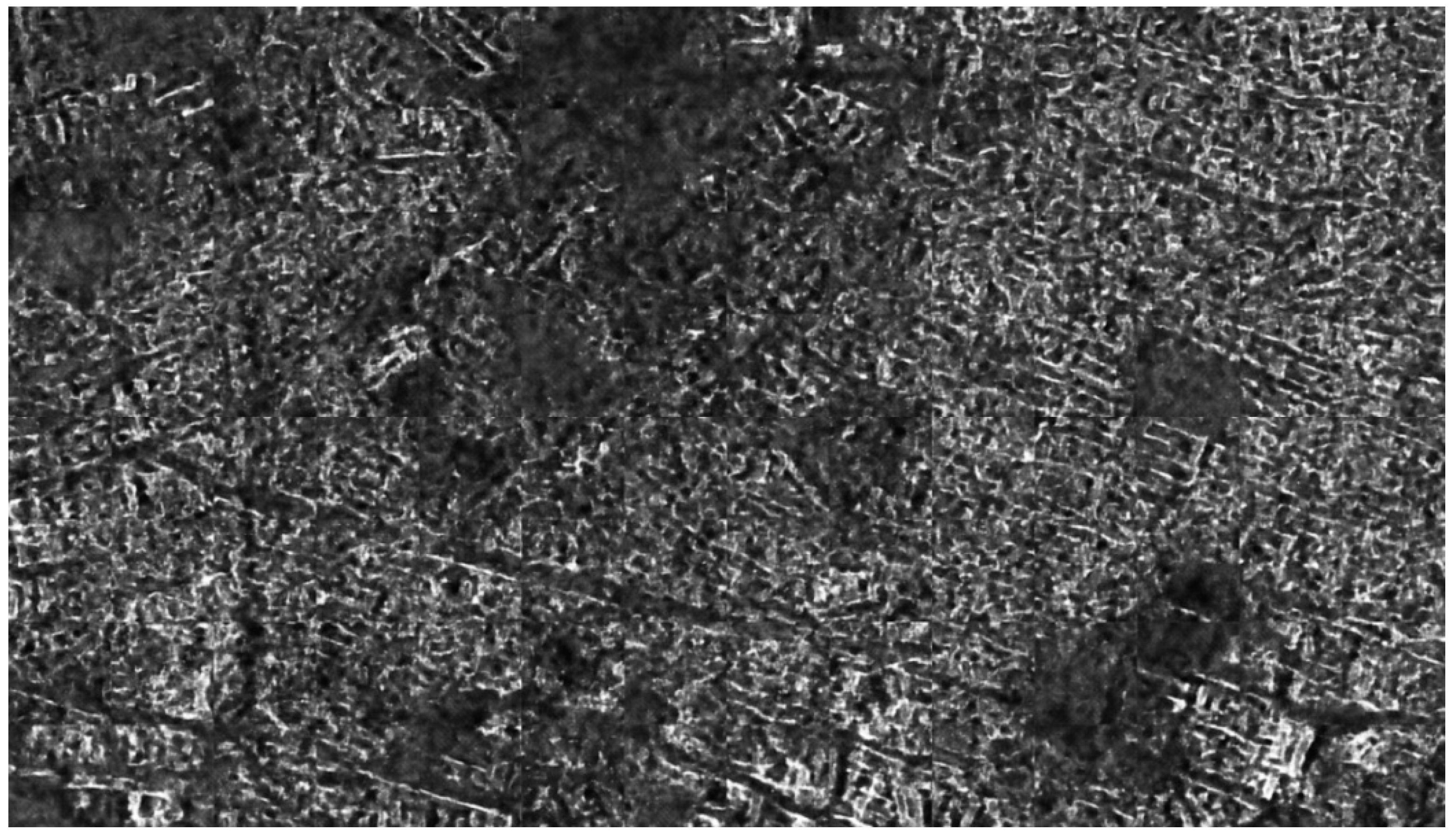
One of the most important merits of remote sensing images is their large-scale observation. In this section, we are discussing how a remote sensing image looks when its patches are processed by the selected neural networks. A full image is generated by concatenating the small processed patches to produce a final image. In this paper, we focus on three networks, our “Dialectical GAN”, the texture network with a Spatial Gram matrix, and the WGAN-GP method. They are shown in Figure 14, Figure 15 and Figure 16, respectively. As for the overall visual performance, we consider that the Dialectical GAN has the best subjective visual performances.

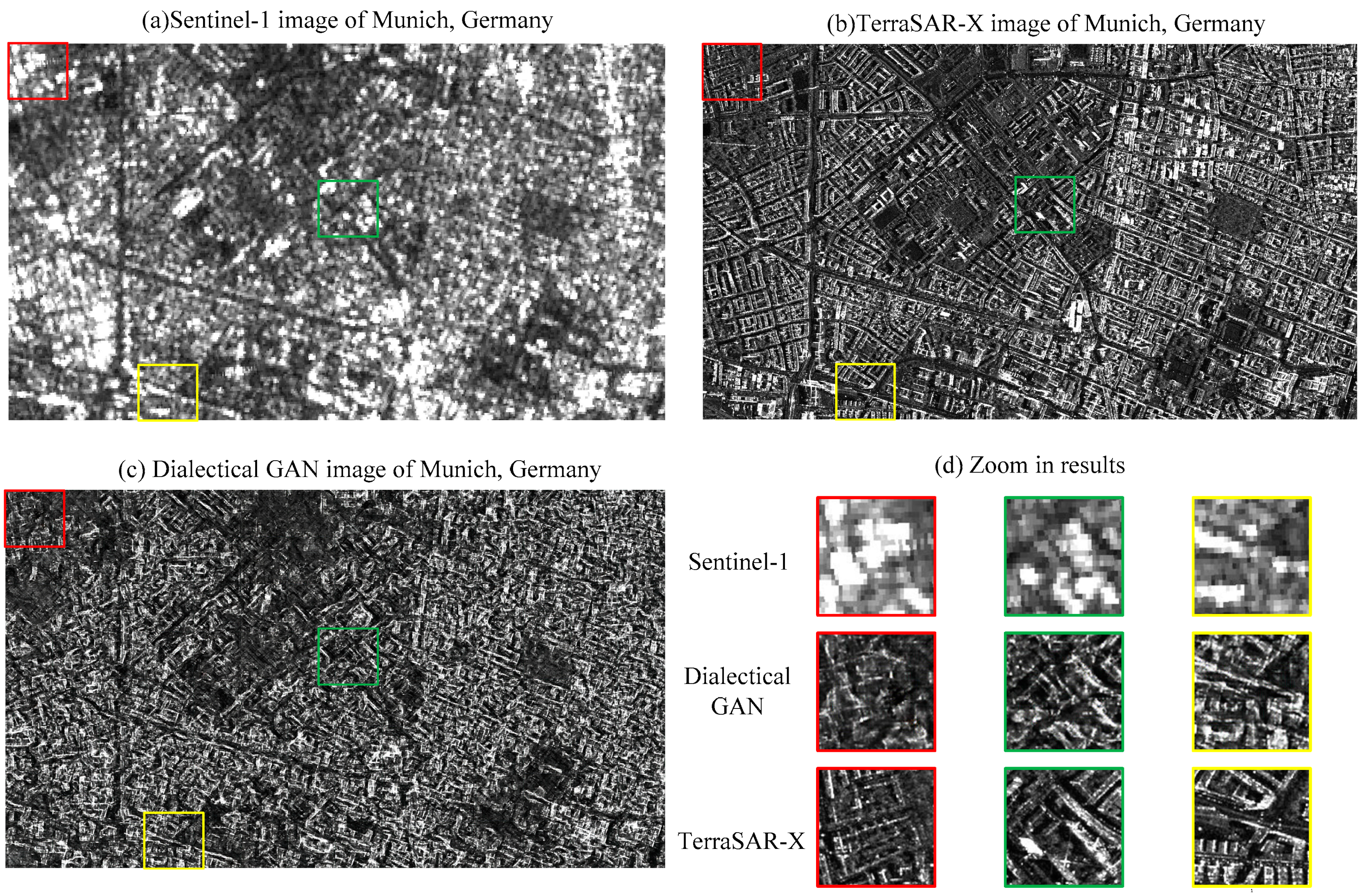
The SAR image translation results compared with inputs and outputs image are shown in Figure 17. First, we can see the entire effect of the image translation in the Munich urban area. To display detail results, we have three bounding boxes with different colors (Red, Green, and Yellow) to extract the patches from the full image. They are in Figure 17d.

6. Discussion

Compared with traditional image enhancement methods, deep learning is an end-to-end method that is quite easy to be implemented. Deep learning has excellent performances and is standing out among machine learning algorithms, especially in the case of big data. Solutions for remote sensing applications were discovered by the advent of deep learning. More importantly, deep learning is now playing a crucial role in transferring the style of images.

Concerning SAR image translation, little attention has been focused on it and the performances of deep learning on this topic are still unknown. The task addressed in this paper is related to super-resolution tasks, but our image pairs are not of the same appearances due to the differences in incidence angles, radar polarization, and acquisition times. From this aspect, our task belongs to style transfer to some extent, like generating a piece of artistic painting without the constraint that the two images should be focused on the same objects. Therefore, SAR image translation is a mix of super-resolution and style transfer and has never been focused on the previous conception of deep learning.

From Gatys et al.’s method to GAN frameworks, we have tested the capabilities of deep learning in translating Sentinel-1 images to TerraSAR-X images. The resulting images of Gatys et al.’s method are of high quality, but they don’t preserve structure information well, which is an essential characteristic of SAR images, especially for urban areas. The improvement can be accomplished by introducing Spatial Gram matrices instead of the traditional ones in the loss function. A Spatial Gram matrix is a compromise between the arrangement structure and the freedom of style. In this paper, we composed Gram matrices computed in spatial shifting mode as a new matrix-vector for each layer. The spatial matrix is a good indicator to describe arrangement structures, such as buildings and roads. However, our loss function modifications can only solve the style presentation problem, but the high computation effort still limits the applications of image translation for remote sensing. Fortunately, deep neural networks are a powerful tool for fitting complicated functions that provide solutions to speed up image translation. Instead of taking every pixel as a random variable, a deep neural network regards an image as an input of the system, and the only thing deep learning can do is to approximate the mapping function. That is to say, the deep neural network is a Generator, and the Spatial Gram matrix is used to define the loss function.

The GAN framework gives us a new concept of a loss function which can also be defined by a neural network, called a “Discriminator”. We assumed that the GAN framework has a dialectical logical structure and explained it in a triad. However, due to the arbitrariness of a neural network and the limitation of the training data, it is hard to train a GAN and the trained GAN cannot usually achieve good performances for our applications. Considering the diversity of GANs and the determinacy of Spatial Gram matrices, we proposed a new method that combines their advantages together. With the initial loss function defined by Spatial Gram matrices, our GAN system updates its Discriminator and Generator to make the output image as “true” as possible. The Spatial Gram loss function works well, but we still believe that there are other functions to determine the style of a given image. Using a combination framework, our system is able to generate high-quality SAR images and to improve the resolutions of Sentinel-1 images without the need for large amounts of data.

To appraise the generated images, we used three indicators, MSE, SSIM, and ENL. The comparison experiments show that the Spatial Gram matrix is better than the traditional Gram matrix. A WGAN-GP without any initial loss function didn’t perform well in contrast to the Spatial Gram matrix method. With the support of Spatial Gram matrices, the new WGAN-GP that we proposed is the best of these three methods, both in visual performance and by quantitative measurements (using the three indicators). Additionally, we have tested the overall visual performance rather than staying at image patch level. It is a new attempt for deep learning to perform the image transfer task in this way. The same results occurred when full images were considered and the new proposed method outperforms the existing ones. However, there will be some fake targets or some targets are missing in the generated images. These errors are the drawbacks of the GAN method and it is hard to use an exact theory to explain why they occur. One of the solutions might be increasing the training data. Explaining the behavior of the deep neural network is still a tough issue that needs to be studied.

Our method gives a solution for SAR image translation, but it is not a substitute for traditional SAR imaging algorithms or SAR hardware systems. With the high-resolution images generated by traditional methods, the deep learning method can learn from them and produce impressive results. The data are always the foundation of the deep learning method. We just use the dialectic to learn some laws from the various appearances.

7. Conclusions

In this paper, a “Dialectical GAN” based on Spatial Gram matrices and a WGAN-GP framework was proposed to conduct the SAR image transfer task from Sentinel-1 to TerraSAR-X images. By analyzing the behavior of SAR images in the VGG-19 pretrained network, we found that the relationship between two source images is maintained in the higher layers of the VGG-19 network, which is the foundation of changing the “style” of images. In remote sensing, the urban areas are usually dominated by buildings and roads, and based on this observation, the Spatial Gram matrices are a very good metric to describe the “style” information of these areas, including their arrangement structure.

In order to explain the idea of a GAN, we introduced the dialectical way and adapted each part of the proposed frame to fit with this logical structure. The proposed method is combining the loss functions of Spatial Gram and WGAN-GP methods to meet our requirements. The results of the translation show promising capabilities, especially for urban areas. The networks learn an adaptive loss from image pairs at hand and are regularized by the prescribed image style, which makes it applicable for the task of SAR image translation.

For future works, we plan to go into deeper mathematic details and explanations of the Dialectical GAN. The combination of radar signal theory and deep learning needs to be investigated in order to describe the change of the basic unit (e.g., point spread function). In addition, this paper is limited to the application of SAR image translations, now we are trying to understand the translation of SAR, and optical images. In the future, we would like to apply our techniques to other target areas and other sensors.

References

- Love, A. In memory of Carl A. Wiley. IEEE Antennas Propag. Soc. Newsl. 1985, 27, 17–18. [Google Scholar] [CrossRef]
- TerraSAR-X—Germany’s Radar Eye in Space. Available online: https://www.dlr.de/dlr/en/desktopdefault.aspx/tabid-10377/565_read-436/#/gallery/3501 (accessed on 18 May 2018).
- TanDEM-X—The Earth in Three Dimensions. Available online: https://www.dlr.de/dlr/en/desktopdefault.aspx/tabid-10378/566_read-426/#/gallery/345G (accessed on 18 May 2018).
- RADARSAT. Available online: https://en.wikipedia.org/wiki/RADARSAT (accessed on 18 May 2018).
- COSMO-SkyMed. Available online: http://en.wikipedia.org/wiki/COSMO-SkyMed (accessed on 18 May 2018).
- European Space Agency. Available online: http://en.wikipedia.org/wiki/European_Space_Agency (accessed on 18 May 2018).
- Li, Y.H.; Guarnieri, A.M.; Hu, C.; Rocca, F. Performance and Requirements of GEO SAR Systems in the Presence of Radio Frequency Interferences. Remote Sens. 2018, 10, 82. [Google Scholar] [CrossRef]
- Ao, D.Y.; Li, Y.H.; Hu, C.; Tian, W.M. Accurate Analysis of Target Characteristic in Bistatic SAR Images: A Dihedral Corner Reflectors Case. Sensors 2018, 18, 24. [Google Scholar] [CrossRef] [PubMed]
- Gatys, L.A.; Ecker, A.S.; Bethge, M. Image style transfer using convolutional neural networks. In Proceedings of the IEEE Conference on Computer Vision and Pattern Recognition (CVPR), Las Vegas, NV, USA, 27–30 June 2016; pp. 2414–2423. [Google Scholar]
- Ulyanov, D.; Lebedev, V.; Vedaldi, A.; Lempitsky, V.S. Texture Networks: Feed-forward Synthesis of Textures and Stylized Images. arXiv, 2016; arXiv:1603.03417. [Google Scholar]
- Johnson, J.; Alahi, A.; Fei-Fei, L. Perceptual losses for real-time style transfer and super-resolution. In Proceedings of the European Conference on Computer Vision, Amsterdam, The Netherlands, 11–14 October 2016; pp. 694–711. [Google Scholar]
- Goodfellow, I.; Pouget-Abadie, J.; Mirza, M.; Xu, B.; Warde-Farley, D.; Ozair, S.; Courville, A.; Bengio, Y. Generative adversarial nets. In Proceedings of the Advances in Neural Information Processing Systems, Montreal, QC, Canada, 8–12 December 2014; pp. 2672–2680. [Google Scholar]
- Isola, P.; Zhu, J.-Y.; Zhou, T.; Efros, A.A. Image-to-image translation with conditional adversarial networks. arXiv, 2017; arXiv:1611.07004. [Google Scholar]
- Merkle, N.; Auer, S.; Müller, R.; Reinartz, P. Exploring the Potential of Conditional Adversarial Networks for Optical and SAR Image Matching. IEEE J. Sel. Top. Appl. Earth Obs. Remote Sens. 2018, 11, 1811–1820. [Google Scholar] [CrossRef]
- Zhu, X.X.; Tuia, D.; Mou, L.; Xia, G.-S.; Zhang, L.; Xu, F.; Fraundorfer, F. Deep learning in remote sensing: A review. arXiv, 2017; arXiv:1710.03959. [Google Scholar]
- Garcia-Pineda, O.; Zimmer, B.; Howard, M.; Pichel, W.; Li, X.; MacDonald, I.R. Using SAR Image to Delineate Ocean Oil Slicks with a Texture Classifying Neural Network Algorithm (TCNNA). Can. J. Remote Sens. 2009, 5, 411–421. [Google Scholar] [CrossRef]
- Shi, H.; Chen, L.; Zhuang, Y.; Yang, J.; Yang, Z. A novel method of speckle reduction and enhancement for SAR image. In Proceedings of the IEEE International Geoscience and Remote Sensing Symposium (IGARSS), Fort Worth, TX, USA, 23–28 July 2017; pp. 3128–3131. [Google Scholar]
- Chierchia, G. SAR image despeckling through convolutional neural networks. In Proceedings of the 2017 IEEE International Geoscience and Remote Sensing Symposium (IGARSS), Fort Worth, TX, USA, 23–28 July 2017. [Google Scholar]
- Xiang, D.; Tang, T.; Hu, C.; Li, Y.; Su, Y. A kernel clustering algorithm with fuzzy factor: Application to SAR image segmentation. IEEE Geosci. Remote Sens. Lett. 2014, 11, 1290–1294. [Google Scholar] [CrossRef]
- Hu, C.; Li, Y.; Dong, X.; Wang, R.; Cui, C. Optimal 3D deformation measuring in inclined geosynchronous orbit SAR differential interferometry. Sci. China Inf. Sci. 2017, 60, 060303. [Google Scholar] [CrossRef]
- Sentinel-1. Available online: http://en.wikipedia.org/wiki/Sentinel-1 (accessed on 18 May 2018).
- TerraSAR-X. Available online: http://en.wikipedia.org/wiki/ TerraSAR-X (accessed on 18 May 2018).
- Ao, D.; Wang, R.; Hu, C.; Li, Y. A Sparse SAR Imaging Method Based on Multiple Measurement Vectors Model. Remote Sens. 2017, 9, 297. [Google Scholar] [CrossRef]
- Mitas, L.; Mitasova, H. Spatial Interpolation. In Geographical Information Systems: Principles, Techniques, Management and Applications; Longley, P., Goodchild, M.F., Maguire, D.J., Rhind, D.W., Eds.; Wiley: Hoboken, NJ, USA, 1999. [Google Scholar]
- Dumitru, C.O.; Schwarz, G.; Datcu, M. Land cover semantic annotation derived from high-resolution SAR images. IEEE J. Sel. Top. Appl. Earth Obs. Remote Sens. 2016, 9, 2215–2232. [Google Scholar] [CrossRef]
- Jing, Y.; Yang, Y.; Feng, Z.; Ye, J.; Yu, Y.; Song, M. Neural style transfer: A review. arXiv, 2017; arXiv:1705.04058. [Google Scholar]
- Liao, J.; Yao, Y.; Yuan, L.; Hua, G.; Kang, S.B. Visual attribute transfer through deep image analogy. arXiv, 2017; arXiv:1705.01088. [Google Scholar] [CrossRef]
- Berger, G.; Memisevic, R. Incorporating long-range consistency in CNN-based texture generation. arXiv, 2016; arXiv:1606.01286. [Google Scholar]
- The-Gan-Zoo. Available online: http://github.com/hindupuravinash/the-gan-zoo (accessed on 18 May 2018).
- Li, C.; Wand, M. Precomputed real-time texture synthesis with Markovian generative adversarial networks. In Proceedings of the European Conference on Computer Vision, Amsterdam, The Netherlands, 11–14 October 2016; pp. 702–716. [Google Scholar]
- Ledig, C.; Theis, L.; Huszár, F.; Caballero, J.; Cunningham, A.; Acosta, A.; Aitken, A.; Tejani, A.; Totz, J.; Wang, Z.; et al. Photo-realistic single image super-resolution using a generative adversarial network. arXiv, 2016; arXiv:1609.04802. [Google Scholar]
- Pathak, D.; Krahenbuhl, P.; Donahue, J.; Darrell, T.; Efros, A.A. Context encoders: Feature learning by inpainting. In Proceedings of the IEEE Conference on Computer Vision and Pattern Recognition, Amsterdam, The Netherlands, 11–14 October 2016; pp. 2536–2544. [Google Scholar]
- Zhu, J.-Y.; Krähenbühl, P.; Shechtman, E.; Efros, A.A. Generative visual manipulation on the natural image manifold. In Proceedings of the European Conference on Computer Vision, Amsterdam, The Netherlands, 11–14 October 2016; pp. 597–613. [Google Scholar]
- Schnitker, S.A.; Emmons, R.A. Hegel’s Thesis-Antithesis-Synthesis Model. In Encyclopedia of Sciences and Religions; Runehov, A.L.C., Oviedo, L., Eds.; Springer: Dordrecht, The Netherlands, 2013. [Google Scholar]
- Liang, S.; Srikant, R. Why deep neural networks for function approximation? arXiv, 2016; arXiv:1610.04161. [Google Scholar]
- Yarotsky, D. Optimal approximation of continuous functions by very deep ReLU networks. arXiv, 2018; arXiv:1802.03620. [Google Scholar]
- Wang, X.; Gupta, A. Generative image modeling using style and structure adversarial networks. In Proceedings of the European Conference on Computer Vision, Amsterdam, The Netherlands, 11–14 October 2016; pp. 318–335. [Google Scholar]
- Hinton, G.E.; Salakhutdinov, R.R. Reducing the dimensionality of data with neural networks. Science 2006, 313, 504–507. [Google Scholar] [CrossRef] [PubMed]
- Metric Space. Available online: https://en.wikipedia.org/wiki/Metric_space (accessed on 18 May 2018).
- Nowozin, S.; Cseke, B.; Tomioka, R. f-gan: Training generative neural samplers using variational divergence minimization. arXiv, 2016; arXiv:1606.00709. [Google Scholar]
- Divergence (Statistics). Available online: https://en.wikipedia.org/wiki/ Divergence_(statistics) (accessed on 18 May 2018).
- Mao, X.; Li, Q.; Xie, H.; Lau, R.Y.; Wang, Z.; Smolley, S.P. Least squares generative adversarial networks. In Proceedings of the IEEE International Conference on Computer Vision (ICCV), Tampa, FL, USA, 5–8 December 1988; pp. 2813–2821. [Google Scholar]
- Arjovsky, M.; Chintala, S.; Bottou, L. Wasserstein gan. arXiv, 2017; arXiv:1701.07875. [Google Scholar]
- Gulrajani, I.; Ahmed, F.; Arjovsky, M.; Dumoulin, V.; Courville, A.C. Improved training of wasserstein gans. arXiv, 2017; arXiv:1704.00028. [Google Scholar]
- Pennington, J.; Bahri, Y. Geometry of neural network loss surfaces via random matrix theory. In Proceedings of the International Conference on Machine Learning, Sydney, Australia, 6–11 August 2017; pp. 2798–2806. [Google Scholar]
- Haeffele, B.D.; Vidal, R. Global optimality in neural network training. In Proceedings of the IEEE Conference on Computer Vision and Pattern Recognition, Tampa, FL, USA, 5–8 December 1988; pp. 7331–7339. [Google Scholar]
- Lucic, M.; Kurach, K.; Michalski, M.; Gelly, S.; Bousquet, O. Are GANs Created Equal? A Large-Scale Study. arXiv, 2017; arXiv:1711.10337. [Google Scholar]
- Wang, Z.; Bovik, A.C.; Sheikh, H.R.; Simoncelli, E.P. Image quality assessment: from error visibility to structural similarity. IEEE Trans. Image Process. 2004, 13, 600–612. [Google Scholar] [CrossRef] [PubMed]
- Zénere, M.P. SAR Image Quality Assessment; Universidad Nacional De Cordoba: Córdoba, Argentina, 2012. [Google Scholar]
- Anfinsen, S.N.; Doulgeris, A.P.; Eltoft, T. Estimation of the equivalent number of looks in polarimetric synthetic aperture radar imagery. IEEE Trans. Geosci. Remote Sens. 2009, 47, 3795–3809. [Google Scholar] [CrossRef]
Figure 1.
Visualization of Sentinel-1 and TerraSAR-X Synthetic Aperture Radar (SAR) images in the Visual Geometry Group (VGG)-19 layers.
Figure 2.
Experiment using the Gatys et al. method. (a) Content image (Sentinel-1); (b) transferred image (Gram matrix); (c) style image (TerraSAR-X).
Figure 3.
Experiment using Spatial Gram matrices. (a) Content image (Sentinel-1); (b) transferred image (Spatial Gram matrix); (c) transferred image (Gatys et al.’s Gram matrix); (d) style image (TerraSAR-X).
Figure 4.
SAR image translation using the “pix2pix” framework in both training and test set. (a) Input image in the training set; (b) Generative Adversarial Network (GAN) output of image a; (c) target of image a; (d) input image in the test set; (e) GAN output of image d; (f) target of image d.
Figure 5.
Global flowchart of Dialectical GAN.
Figure 6.
Architecture of the “U-Net” Generator network.
Figure 7.
Architecture of the PatchGAN Discriminator network.
Figure 8.
Two image patch-pairs input to in the VGG-19 networks and their intermediate results.
Figure 9.
Style transfer experiments with different content layers.
Figure 10.
Comparison between a Berger et al. Spatial Gram matrix and a Gatys et al. Gram matrix in two patch-pairs.
Figure 11.
Comparison between Texture network and Wasserstein Generative Adversarial Network—Gradient Penalty (WGAN-GP) for two patch-pairs.
Figure 12.
Comparison between Dialectical GAN and Texture network for two image patch-pairs.
Figure 13.
Comparison of three images of a line target at signal level.
Figure 14.
The overall results of a Dialectical-GAN.
Figure 15.
The overall results of a texture network.
Figure 16.
The overall results of a WGAN-GP (L1 +WGAN-GP).
Figure 17.
Overall visual performance of Dialectical GAN compared with Sentinel-1 and TerraSAR-X images. (a) Sentinel-1 image; (b) TerraSAR-X image; (c) Dialectical GAN image; (d) zoom in results.