LDAS-Monde Sequential Assimilation of Satellite Derived Observations Applied to the Contiguous US: An ERA-5 Driven Reanalysis of the Land Surface Variables

Abstract

Land data assimilation system (LDAS)-Monde, an offline land data assimilation system with global capacity, is applied over the CONtiguous US (CONUS) domain to enhance monitoring accuracy for water and energy states and fluxes. LDAS-Monde ingests satellite-derived surface soil moisture (SSM) and leaf area index (LAI) estimates to constrain the interactions between soil, biosphere, and atmosphere (ISBA) land surface model (LSM) coupled with the CNRM (Centre National de Recherches Météorologiques) version of the total runoff integrating pathways (CTRIP) continental hydrological system (ISBA-CTRIP). LDAS-Monde is forced by the ERA-5 atmospheric reanalysis from the European Center for Medium Range Weather Forecast (ECMWF) from 2010 to 2016 leading to a seven-year, quarter degree spatial resolution offline reanalysis of land surface variables (LSVs) over CONUS. The impact of assimilating LAI and SSM into LDAS-Monde is assessed over North America, by comparison to satellite-driven model estimates of land evapotranspiration from the Global Land Evaporation Amsterdam Model (GLEAM) project, and upscaled ground-based observations of gross primary productivity from the FLUXCOM project. Taking advantage of the relatively dense data networks over CONUS, we have also evaluated the impact of the assimilation against in situ measurements of soil moisture from the USCRN (US Climate Reference Network), together with river discharges from the United States Geological Survey (USGS) and the Global Runoff Data Centre (GRDC). Those data sets highlight the added value of assimilating satellite derived observations compared with an open-loop simulation (i.e., no assimilation). It is shown that LDAS-Monde has the ability not only to monitor land surface variables but also to forecast them, by providing improved initial conditions, which impacts persist through time. LDAS-Monde reanalysis also has the potential to be used to monitor extreme events like agricultural drought. Finally, limitations related to LDAS-Monde and current satellite-derived observations are exposed as well as several insights on how to use alternative datasets to analyze soil moisture and vegetation state.

1. Introduction

One of the major scientific challenges in relation to the adaptation to climate change is observing and simulating the response of land biophysical variables to extreme events, making land surface models (LSMs) constrained by high-quality gridded atmospheric variables and coupled with river-routing models key tools to address these challenges [1,2]. The modelling of terrestrial variables can be improved through the dynamical integration of observations. Remote sensing observations are particularly useful in this context because of their global coverage and higher spatial resolution (10 km and below). The current fleet of Earth observation missions holds an unprecedented potential to quantify land surface variables (LSVs) [3] and many satellite-derived products relevant to the hydrological and vegetation cycles are already available at high spatial resolutions. However, satellite remote sensing observations exhibit spatial and temporal gaps and not all key LSVs can be observed. LSMs are able to provide LSV estimates at all times and locations using physically-based equations, but as remotely sensed observations, they are affected by uncertainties (e.g., parametrization representation, atmospheric forcing, initialisation). Through a weighted combination of both, LSVs can be better estimated than by either source of information alone [4]; data assimilation techniques enable one to spatially and temporally integrate observed information into LSMs in a consistent way to unobserved locations, time steps, and variables.

In the past recent years, several land data assimilation system (LDAS) have emerged at different spatial scales: “site level”, like the data assimilation system for LSMs using CLM4.5 (Community Land Model 4.5, [5]); regional, like the coupled land vegetation LDAS (CLVLDAS, [6,7]) and the famine early warning systems network (FEWSNET) LDAS (FLDAS, [8]); continental, like the North American LDAS (NLDAS, [9,10]) and the National Climate Assessment LDAS (NCA-LDAS [11]); as well as at global scale, like the global land data assimilation (GLDAS, [12]) and, more recently, LDAS-Monde [13]. LDAS-Monde has been developed to constrain the CO₂-responsive version of the ISBA (interactions between soil, biosphere, and atmosphere) LSM [14,15,16,17] using satellite derived observations within the open-source SURFEX modelling platform (SURFace Externalisee, [18]) of Meteo-France. LDAS-Monde has been implemented in a monitoring chain of terrestrial water and carbon fluxes. Unlike most of the above mentioned LDAS, LDAS-Monde is able to jointly and sequentially assimilate vegetation products such as leaf area index (LAI) together with surface soil moisture (SSM) observations [13,19,20,21]. Ref. [13] tested LDAS-Monde over Europe and the Mediterranean basin for the 2000–2012 period. A long term, global scale, multi-sensor satellite-derived surface soil moisture dataset (ESA CCI SSM, [22,23,24,25]) along with satellite derived LAI (GEOV1, http://land.copernicus.eu/global/ last access, June 2018), were jointly assimilated. LDAS-Monde was forced by WFDEI (WATCH-forcing-data-ERA-interim) observations based atmospheric forcing dataset [26,27] at half degree spatial resolution. Analysis impact was successfully carried out using (i) agricultural statistics over France; (ii) river discharge observations; (iii) satellite-derived estimates of land evapotranspiration from the global land evaporation amsterdam model (GLEAM) project; and (iv) spatially gridded observations-based estimates of up-scaled gross primary production and evapotranspiration from the FLUXNET network [13].

In this study, LDAS-Monde is applied and tested in a data-rich area: the CONtiguous US (CONUS, defined here as longitudes from 130.0°W to 60.0°W, latitudes from 20.0°N to 55.0°N, as shown in Figure 1). LDAS-Monde is forced by the latest ERA-5 atmospheric reanalysis from the European Center for Medium Range Weather Forecast (ECMWF) from 2010 to 2016 leading to a seven-year, quarter degree spatial resolution offline reanalysis of the land surface variables (LSVs). Ref. [28] assessed ERA-5 ability to force the ISBA LSM by comparison to satellite-derived products and in situ observations covering a substantial part of the land surface storage and fluxes. They found that using ERA-5 in place of its predecessor, ERA-Interim, led to significant improvements in the representation of the LSVs linked to the terrestrial water cycle (surface soil moisture, river discharges, snow depth, and turbulent atmospheric fluxes), but did not improve the LSVs linked to the vegetation cycle (evapotranspiration, carbon uptake, and LAI). In that respect, the assimilation of LAI through ERA-5 driven reanalysis from LDAS-Monde is expected to bring clear improvements [13]. In this study, the impact of LDAS-Monde analysis with respect to an open-loop (i.e., model run without assimilation) is assessed using satellite-driven model estimates of land evapotranspiration from the Global Land Evaporation Amsterdam Model (GLEAM) project and upscaled ground-based observations of gross primary productivity from the FLUXCOM project, together with river discharges from the United States Geophysical Survey (USGS) and the Global Runoff Data Centre (GRDC). Over CONUS, in situ measurements of soil moisture from the USCRN network (US Climate Reference Network) are also used in the evaluation. Section 2 describes the different components of LDAS-Monde as well as the evaluation data sets and strategy. Section 3 provides a set of statistical diagnostics to assess and evaluate the impact of the assimilation. Finally, Section 4 provides perspectives and future research directions.

2. Data and Methods

2.1. LDAS-Monde System Components

LDAS-Monde allows sequential assimilation of satellite derived land observations at a global scale. The assimilation is performed into the open-access SURFEX modelling platform of Météo-France (SURFace Externalisée, [18]). It produces offline re-analyses of LSVs using (i) an LSM along with data assimilation techniques, (ii) observations, and (iii) atmospheric forcing. Those components of LDAS-Monde are briefly described below.

2.1.1. The SURFEX Modelling Platform

LDAS-Monde uses the CO₂-responsive version of ISBA embedded within the SURFEX platform. The most recent version of SURFEX (version 8.1) is used in this study with the “NIT” plant biomass monitoring option for ISBA. In this configuration, ISBA simulates leaf-scale physiological processes and plant growth [15,16,17]. The dynamic evolution of the vegetation biomass and LAI variables is driven by photosynthesis in response to atmospheric and climate conditions. Photosynthesis enables vegetation growth resulting from the CO₂ uptake. During the growing phase, enhanced photosynthesis corresponds to a CO₂ uptake, which results in vegetation growth from the LAI minimum threshold (prescribed as 1 m² m⁻² for coniferous forest or 0.3 m² m⁻² for other vegetation types). Transfers of water and heat through the soil rely on a multilayer diffusion scheme [29,30]. The ISBA parameters are defined for 12 generic land surface patches. They include nine plant functional types (needle leaf trees, evergreen broadleaf trees, deciduous broadleaf trees, C3 crops, C4 crops, C4 irrigated crops, herbaceous, tropical herbaceous, and wetlands) as well as bare soil, rocks, and permanent snow and ice surfaces.

This version of ISBA is coupled to the CTRIP river routing model through OASIS-MCT [31] in order to simulate streamflows of the main rivers [32,33,34,35]. Besides, a single-source energy budget of a soil/vegetation composite is computed. SURFEX also involves data assimilation techniques to analyse LSVs from the ISBA LSM.

This study makes use of the simplified version of an extended Kalman filter (SEKF), as already used and described in [13,19,21,36]. The SEKF uses finite differences from perturbed simulations to estimate the linear tangent model linking the model state control variables to the observed variables. Satellite derived surface soil moisture (SSM) and leaf area index (LAI) are simultaneously assimilated to update eight model state control variables (i.e., control variables); LAI and soil moisture from seven layers of soil, from 1 cm to 100 cm. Assimilating SSM and LAI within LDAS-Monde results in updates of the LSM variables in different ways. Model variables corresponding to the observations are first updated through the Kalman gain computed by the SEKF. Secondly, control variables are updated through their sensitivity to the observed variables. For example, the assimilation of LAI impacts LAI itself, but also soil moisture from the seven layers present in the state vector and the assimilation of SSM impacts LAI. Finally, other variables are indirectly modified by the analysis through biophysical processes and feedbacks in the model by updates of the control variables.

2.1.2. ESA CCI Surface Soil Moisture and CGLS Leaf Area Index

In this study the European Space Agency and Climate Change Initiative (ESA CCI) SSM-combined version of the product (v4.1) is assimilated into LDAS-Monde (http://www.esa-soilmoisture-cci.org, last access June 2018). The CCI merges SSM observations from seven different microwave radiometers (SMMR, SSM/I, TMI, ASMR-E, WindSat, AMSR2, SMOS) and four different scatterometers (ERS-1 and 2 AMI, and MetOp-A and B ASCAT) into a single combined data set covering the time period from November 1978 to December 2016. Data are expressed in volumetric (m³ m⁻³) units and quality flags are provided (i.e., snow coverage or temperature below 0° and dense vegetation). For a more comprehensive overview of the product, see [24,25]. Topographic relief is known to negatively affect satellite remote sensing retrievals of SSM [37], hence the time series for pixels whose average altitude exceeds 1500 m above sea level were not accounted for. Data on pixels with urban land cover fractions larger than 15% were discarded too, to limit the effects of artificial surfaces. These thresholds were set according to [13,20,38], who processed satellite-based SSM retrievals for data assimilation experiments with the ISBA LSM. Data are available almost every day with a spatial resolution of 0.25° × 0.25°. To assimilate SSM data, it is important to rescale the observations such that they are consistent with the model climatology [39,40]. Hence, similarly to previous studies, the ESA CCI SSM product has been transformed into the model-equivalent SSM to address possible misspecification of physiographic parameters, such as the wilting point and the field capacity. The linear rescaling approach described in [41] (using the first two moments of the cumulative distribution function, CDF) was used. It consists of a linear rescaling enabling a correction of the differences in the mean and variance of the distribution. It has been applied at a seasonal scale (i.e., for each specific month) following [13].

The GEOV1 LAI is also assimilated. It is produced by the European Copernicus Global Land Service project (http://land.copernicus.eu/global/, last access June 2018). Ref. [42] proposed an evaluation of this product in the context of Numerical Weather Prediction (NWP). LAI observations are retrieved from the SPOT-VGT (from 1999 to 2014) and then from PROBA-V (from 2014 to present) satellite data according to the methodology proposed by [43]. The 1 km spatial resolution observations are interpolated by an arithmetic average to the 0.25° × 0.25° model grid points, if at least 50% of the observation grid points are observed (i.e., half the maximum amount). LAI observations have a temporal frequency of 10 days at best (e.g., in presence of clouds, no observations are available). Both assimilated datasets are illustrated by Figure 1, averaged over 2010–2016.

2.1.3. ERA-5 Atmospheric Reanalysis

ERA-5 [44] is the fifth generation of European re-analyses produced by the ECMWF and a key element of the EU-funded Copernicus Climate Change Service (C3S). ERA-5 important changes relative to ERA-interim former ECMWF’s atmospheric reanalysis include (i) a higher spatial and temporal resolution as well as (ii) a more recent version of ECMWF Earth system model physics and data assimilation system (corresponding to ECMWF’s cycle CY41R2, https://www.ecmwf.int/en/forecasts/documentation-and-support/changes-ecmwf-model/ifs-documentation, last access June 2018). It makes it possible to use modern parameterizations of Earth processes compared with older versions used in ERA-interim. For instance, in addition to being applied to satellite observations, a variational bias scheme is also applied to aircraft and surface ozone and pressure data. ERA-5 also benefits from reprocessed data sets that were not ready yet during the production of ERA-interim. Two other important features of ERA-5 are the more frequent model output and improved model spatial resolution, going from six-hourly output in ERA-interim to hourly output analysis in ERA-5, and from 79 km (horizontal dimension) and 60 levels (vertical dimension) to 31 km and 137 levels in ERA-5. Finally, ERA-5 also provides an estimate of uncertainty through the use of a 10-member ensemble of data assimilations (EDA) at a coarser resolution (63 km horizontal resolution) and three-hourly frequency. ERA-5 is foreseen to replace ERA-interim re-analysis. All ERA-5 atmospheric variables were interpolated at 0.25° × 0.25° spatial resolution. A bilinear interpolation from the native reanalysis grid to the regular grid was made.

2.2. Evaluation Datasets and Methods

The LDAS-Monde analysis impact was assessed with respect to the open-loop model run (i.e., no assimilation). The system was spun-up by running year 2010 twenty times.

Table 1. Set up of the experiments used in this study. ISBA—interactions between soil, biosphere, and atmosphere; DA—data assimilation; SEKF—simplified version of an extended Kalman filter; ESA CCI SSM—European Space Agency and Climate Change Initiative surface soil moisture; LAI—leaf area index; CTRIP—Centre National de Recherches Météorologiques version of the total runoff integrating pathways.

Experiments (Time Period)	Model	Domain & Spatial Resolution	Atmospheric Forcing	DA Method	Assimilated Observations	Model Equivalents of the Observations	Control Variables	Additional Options
Model or Open-loop (2010–2016)	ISBA Multi-layer soil model CO2-responsive version (Interactive vegetation)	CONtiguous US (CONUS), 0.25° × 0.25°	ERA-5	N/A	N/A	N/A	N/A	Coupling with CTRIP (0.5°)
Analysis (2010–2016)	ISBA Multi-layer soil model CO2-responsive version (Interactive vegetation)	CONtiguous US (CONUS), 0.25° × 0.25°	ERA-5	SEKF	SSM (ESA CCI) LAI (GEOV1)	Rescaled WG2 (Second layer of soil (1–4 cm)) LAI	Layers of soil 2 to 8 (WG2 to WG8, 1–100 cm) LAI	Coupling with CTRIP (0.5°)
Ini_Model (2016)	ISBA Multi-layer soil model CO2-responsive version (Interactive vegetation)	CONtiguous US (CONUS), 0.25° × 0.25°	ERA-5	12-month model run starting on 1 January 2016 (initialised by the model simulation, i.e., Open-loop, run from 2010 to 2015)				Coupling with CTRIP (0.5°)
Ini_Analysis (2016)	ISBA Multi-layer soil model CO2-responsive version (Interactive vegetation)	CONtiguous US (CONUS), 0.25° × 0.25°	ERA-5	12-month model run starting on 1 January 2016 (initialised by the analysis run from 2010 to 2015)				Coupling with CTRIP (0.5°)

presents the set up of the different experiments used in this study, the open-loop and the analysis, as well as two additional model runs: (i) Ini_model, a 12-month model run starting on 1 January 2016 (initialised by the model, that is, the openloop with no data assimilation, simulation run from 2010 to 2015); and (ii) Ini_analysis, a 12-month model run initialised by initial conditions from the analysis on 1 January 2016. The two above-mentioned assimilated datasets (ESA CCI SSM and LAI GEOV1) were used as a way to check to what extent the assimilation system was able to produce analyses closer to these two datasets that were assimilated than the open-loop. Then, two independent spatially distributed datasets, namely evapotranspiration from the GLEAM project [45,46] and gross primary production (GPP) from the FLUXCOM project [47,48], were used in the evaluation process. Ground based measurements of soil moisture from the USCRN (US Climate Reference Network, [49]) were also used, along with river discharge observations from the United States Geophysical Survey (USGS) and the Global Runoff Data Centre (GRDC).

The ability of LDAS-Monde to represent SSM, LAI, evapotranspiration, and GPP was assessed using the correlation coefficient (R) and root mean square difference (RMSD). These metrics were applied at a seasonal scale (i.e., for each month) over 2010–2016. For ground-based measurements of SSM, R was calculated for both absolute and anomaly time series in order to remove the strong impact from the SSM seasonal cycle on this specific metric (see e.g., [13,28]). Ground measurements at a depth of 5 cm were compared with soil moisture of the third layer of soil (between 4 and 10 cm depth) from both the model and the analysis for months from April to September over the 2010–2016 time period to avoid frozen conditions. Only stations with significant R values for the two experiments (with p-value < 0.05) were kept for the evaluation.

In order to provide an easier measurement of the added value of the analysis, statistics were also normalized with respect to the model. The so-called normalized information contribution index (NIC as in [28,50]) was applied to the correlation coefficient (Equation (1), for both volumetric and anomaly time-series) and to RMSD (Equation (2)) to quantify the improvement or degradation from the analysis with respect to the model.

$${\mathrm{NIC}}_{\mathrm{R}}=\frac{{\mathrm{R}}_{\left(\mathrm{Analysis}\right)}-{\mathrm{R}}_{\left(\mathrm{Model}\right)}}{1-{\mathrm{R}}_{\left(\mathrm{Model}\right)}}\times 100$$

(1)

$$N_{\mathrm{RMSD}}=\frac{{\mathrm{RMSD}}_{\left(\mathrm{Analyse}\right)}-{\mathrm{RMSD}}_{\left(\mathrm{Model}\right)}}{{\mathrm{RMSD}}_{\left(\mathrm{Model}\right)}}\times 100$$

(2)

NIC scores were then classified according to three categories: (i) negative impact from the analysis with respect to the model with values smaller than −3%, (ii) positive impact from the analysis with respect to the model with values greater than +3%, and (iii) neutral impact from the analysis with respect to the model with values between −3% and 3%.

Over the 2010–2016 time period, river discharge from the analysis and model runs were compared with daily streamflow data from USGS and GRDC. Data were selected for sub-basins with rather large drainage areas (10,000 km² or greater) because of the low resolution of CTRIP (0.5° × 0.5°) and with a long observation time series (48 months or more). As commonly found in the literature, observed and simulated river discharge (Q) data are expressed in m³ s⁻¹. However, given that the observed drainage areas may differ from the simulated ones, specific discharge in mm d⁻¹ (the ratio of Q to the drainage area) was used in this study, similarly to [13,28]. Stations with drainage areas differing by more than 20% from the simulated ones were discarded. Impact on Q was evaluated using the Kling–Gupta Efficiency (KGE, [51]) score:

$$\mathrm{KGE}=1-\sqrt{{\mathrm{RE}}_{\sigma }^2+{\mathrm{RE}}_{\mu }^2+{\left(1-R\right)}^2}$$

(3)

with RE_μ and RE_σ representing the relative error of simulated or analysed mean and standard deviation (Equations (4) and (5)), respectively; R representing the correlation coefficient between the observed discharges and either the modelled or analysed river discharges.

$${\mathrm{RE}}_{\mu }=\frac{{\mathrm{Q}}_{\mu }}{{\mathrm{Q}}_{{\left(\mathrm{obs}.\right)}_{\mu }}}-1$$

(4)

$${\mathrm{RE}}_{\sigma }=\frac{{\mathrm{Q}}_{\sigma }}{{\mathrm{Q}}_{{\left(\mathrm{obs}.\right)}_{\sigma }}}-1$$

(5)

KGE represents the Euclidean distance from the ideal point in the [RE_μ, RE_σ, R] score space. RE_μ, RE_σ, and R constitute a set of mathematically independent metrics quantifying the fit of simulated/analysed discharge time series. At best, Re_μ and RE_σ are equal to 0 and R is equal to 1 (leading to a perfect KGE value of 1), indicating that simulated or analysed time series are identical to the measured one. NIC (Equation (1)) was applied to KGE (Equation (6)) as well, only for stations with KGE values greater than 0. Finally, RE_μ and RE_σ metrics were normalised, following Equation (7), as well as Equation (8) to appreciate the added value from the analysis with respect to the model.

$${\mathrm{NIC}}_{\mathrm{KGE}}=\frac{{\mathrm{KGE}}_{\left(\mathrm{Analysis}\right)}-{\mathrm{KGE}}_{\left(\mathrm{Model}\right)}}{1-{\mathrm{KGE}}_{\left(\mathrm{Model}\right)}}\times 100$$

(6)

$$N_{{\mathrm{RE}}_{\mu }}=\frac{100\ast {\mathrm{RE}}_{{\mu }_{\left(\mathrm{Analysis}\right)}}-{\mathrm{RE}}_{{\mu }_{\left(\mathrm{Model}\right)}}}{{\mathrm{RE}}_{{\mu }_{\left(\mathrm{Model}\right)}}}$$

(7)

$$N_{{\mathrm{RE}}_{\sigma }}=\frac{100\ast {\mathrm{RE}}_{{\sigma }_{\left(\mathrm{Analysis}\right)}}-{\mathrm{RE}}_{{\sigma }_{\left(\mathrm{Model}\right)}}}{{\mathrm{RE}}_{{\sigma }_{\left(\mathrm{Model}\right)}}}$$

(8)

3. Results

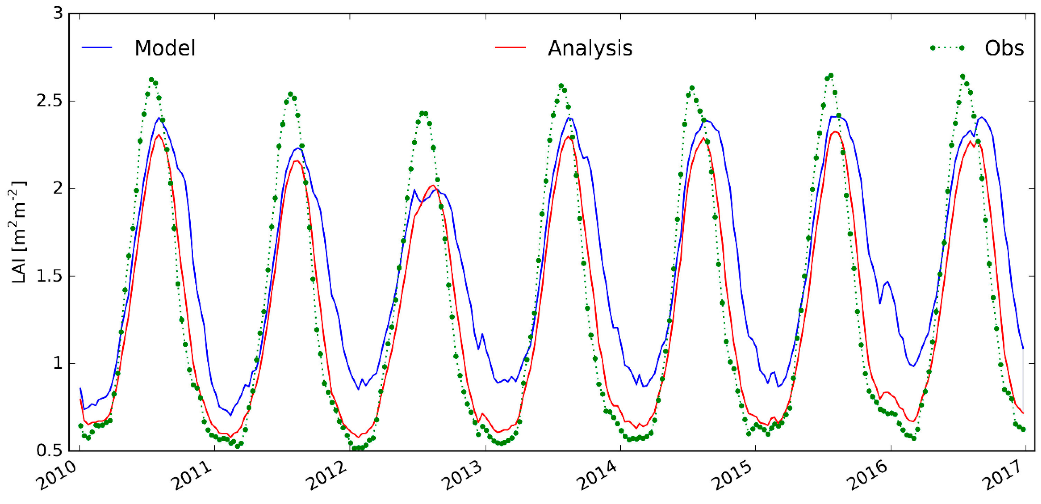
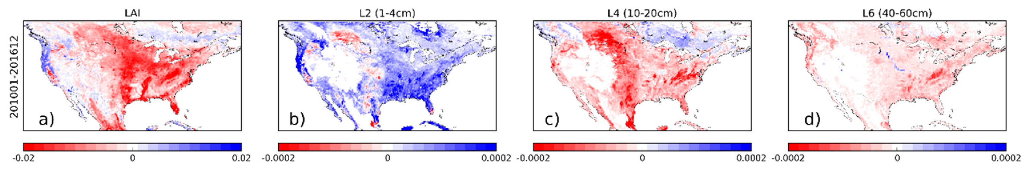
3.1. Analysis Impact on Assimilated Variables

Being the model equivalents of the assimilated observations, LAI and soil moisture from the second layer of soil are expected to be the two variables most affected by the assimilation. Figure 2 presents a 10-day time series of LAI averaged over the whole domain for the 2010–2016 time period. From Figure 2, one can see that the open-loop simulation tends to overestimate the observed LAI in winter periods and that the senescence phase of vegetation is too late over the autumn when compared with the observations. In that respect, the assimilation is efficiently correcting the model; however, analysed LAI does not reach LAI maximal values of the observations. Figure 3 shows maps of LAI for the model (Figure 3a), the observations (Figure 3b), and the analysis (Figure 3c) averaged over 2010–2016. It is clearly visible that the model overestimates LAI in the eastern part of the domain. Also, some geographical patterns visible in the observations (e.g., the Mississippi area in Figure 3b) are not represented in the model (Figure 3a). After assimilation, the analysis presents reduced LAI values in the eastern part of the domain and the above-mentioned geographical patterns are visible too (Figure 3c). This shows the ability of the assimilation to integrate geographical information into the model. Figure 3 also presents seasonal scores between the model and the observations and between the analysis and the observations for RMSD and R over the 2010–2016 time period. The analysis leads to a better fit between the model forecasts and the subsequent assimilated observations for both metrics. On average for the whole period, RMSD values drop from 1.10 m² m⁻² (model vs. observations) to 0.65 m² m⁻² (analysis vs. observations), while R values increase from 0.69 (model vs. observations) to 0.88 (analysis vs. observations). Figure 4 presents the same information content for soil moisture. As ESA CCI SSM was rescaled in order to match the first two moments of the modelled SSM cumulative distribution function, the impact is marginal and differences are hardly visible from Figure 4a–c. From Figure 4d,e, however, one can appreciate the added value of the analysis: RMSD values drop from 0.046 m³ m⁻³ (model vs. observations) to 0.044 m³ m⁻³ (analysis vs. observations), while R values increase from 0.85 (model vs. observations) to 0.87 (analysis vs. observations). It is worth mentioning that the good level of scores (prior as well as after assimilation) are linked to the rescaling of the ESA CCI SSM data to the model climatology. Finally, Figure 5 shows maps of analysis increments for 4 (out of 8) control variables averaged over the whole 2010–2016 time period (LAI, second, fourth, and sixth layers of soil from left to right, respectively). It can be noticed that the magnitude of increments is decreasing with depth. It can also be noticed that over almost the whole domain, the analysis tends to add water in the soil near the surface (positive increments), while it dries layers where the roots are mainly located (from layer 4 to 6, negative increments).

3.2. Evaluation Using Independent Datasets

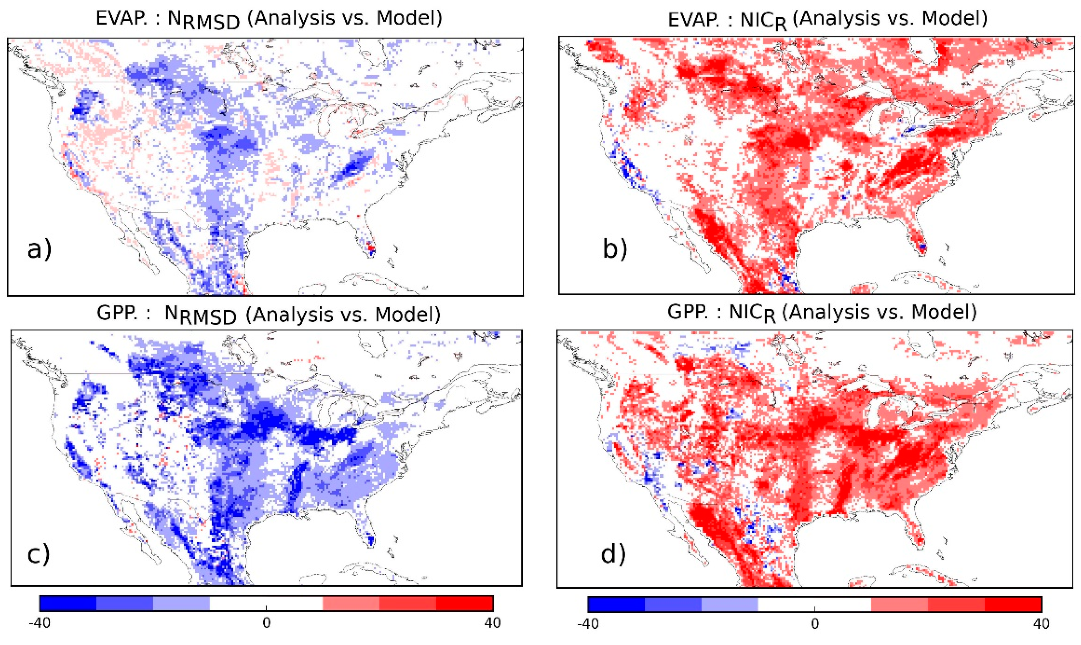
3.2.1. Evapotranspiration and GPP

Table 2. Statistical scores from the evaluation of both the open-loop and the analysis with respect to evapotranspiration and gross primary production (GPP) averaged over 2010–2016. RMSD—root mean square difference.

	Mean of the Evaluation Data Set	Experiments	RMSD	R
Evapotranspiration	1.46 kg/m2/d	Open-loop	0.87 kg/m2/d	0.80
		Analysis	0.85 kg/m2/d	0.81
Gross Primary Production	1.76 g(C)/m2/d	Open-loop	2.20 g(C)/m2/d	0.74
		Analysis	1.91 g(C)/m2/d	0.78

presents the statistical scores from the evaluation of both the open-loop and the analysis with respect to evapotranspiration and GPP averaged over 2010–2016, as well as the mean of the evaluation data set over the considered area. On average, R increases from 0.80 to 0.81 when comparing evapotranspiration from the model and from the analysis, respectively, to the independent estimates. Average RMSD decreases from 0.89 kg m⁻² d⁻¹ to 0.85 kg m⁻² d⁻¹. When compared with GPP estimates, averaged correlations rise from 0.74 to 0.78 and RMSD drops from 2.20 g(C) m⁻² d⁻¹ to 1.91 g(C) m⁻² d⁻¹ when considering the model or the analysis, respectively. Figure 6 presents spatial maps of N_RMSD (Figure 6a,c) and NIC_R (Figure 6b,d) resulting from the comparison with evapotranspiration (Figure 6, top row) and GPP (Figure 6, bottom row) of their modelled and analysed equivalent. For N_RMSD (Figure 6a,c), blue colours represent an improvement from the analysis regarding RMSDs (i.e., the latter better represents either evapotranspiration or GPP than the model), while for NIC_R (Figure 6b,d), red colours depict an improvement from the analysis. Figure 6 shows that both evapotranspiration and GPP are improved almost everywhere in terms of correlation and RMSD, and that the impact of the assimilation is stronger for GPP than for evapotranspiration. At the seasonal scale (not shown), the assimilation leads to a positive impact all year long in the representation of GPP in terms of both RMSD and R values. Impact from the assimilation on evapotranspiration is smaller (as seen in Table 2), while RMSD values are slightly improved all year long, R values are slightly improved from April to October and slightly degraded from November to March.

Geographical patterns, as seen on the middle of Figure 6a,c (transition from relative wet to dry areas) areas of the Midwest, are also visible in the soil moisture increments maps of Figure 5b,c, where stronger increments occur. It is difficult to state whether or not those strong corrections reflect atmospheric forcing errors, for example, precipitation, in this area as to date, very few studies have evaluated ERA5 precipitation errors. Ref. [52] have evaluated a large amount of precipitation products, including ERA5, using the high-resolution (4 km) stage-IV gauge-radar precipitation data set as a reference over CONUS using several metrics for 2008–2017. Figure 1d of [52], illustrates the Kling–Gupta efficiency (KGE) scores between ERA5 precipitation and stage-IV reference. If lower values seem to be observed in the above-mentioned transition area, it is not clear enough to incriminate precipitation errors. However, this geographical pattern corresponds to a specific soil moisture regime, the Ustic regime, where moisture is present in the soil, but limited, at times in which conditions are suitable for plant growth (as visible on the following USDA map: https://www.nrcs.usda.gov/Internet/FSE_MEDIA/nrcs142p2_050436.jpg, last access October 2018). This area has specific soil properties including clay, with high swelling potential [53]. Such soil properties are likely to be misrepresented in the model, possibly leading to stronger increments in the analysis.

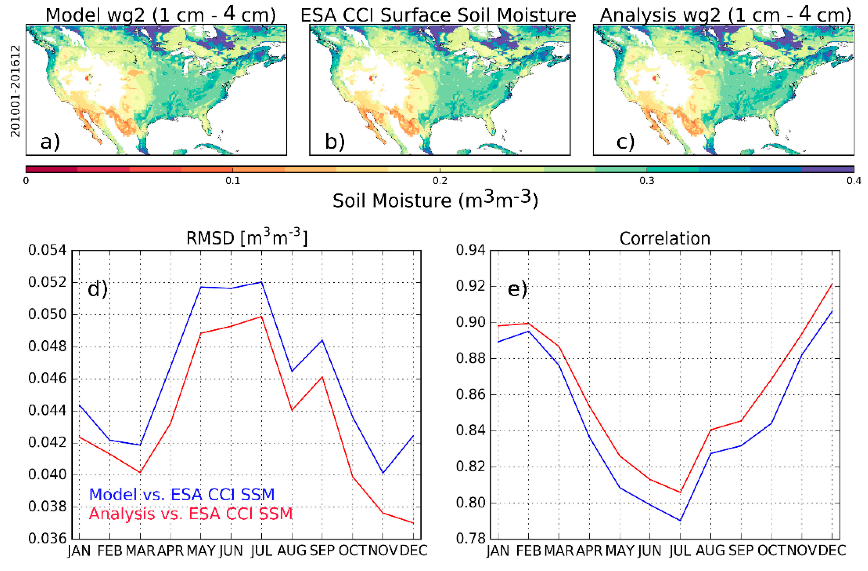
3.2.2. Soil Moisture

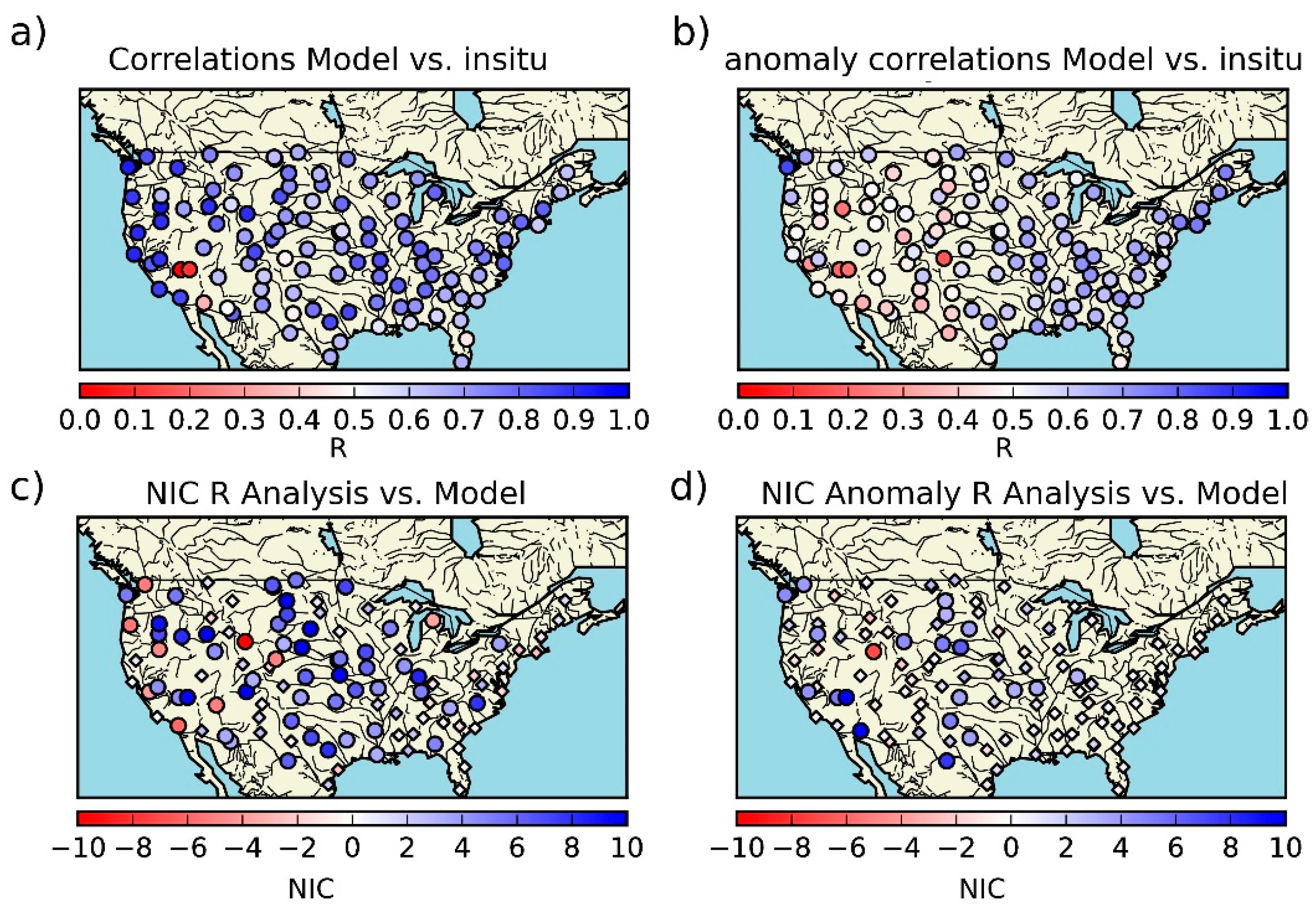
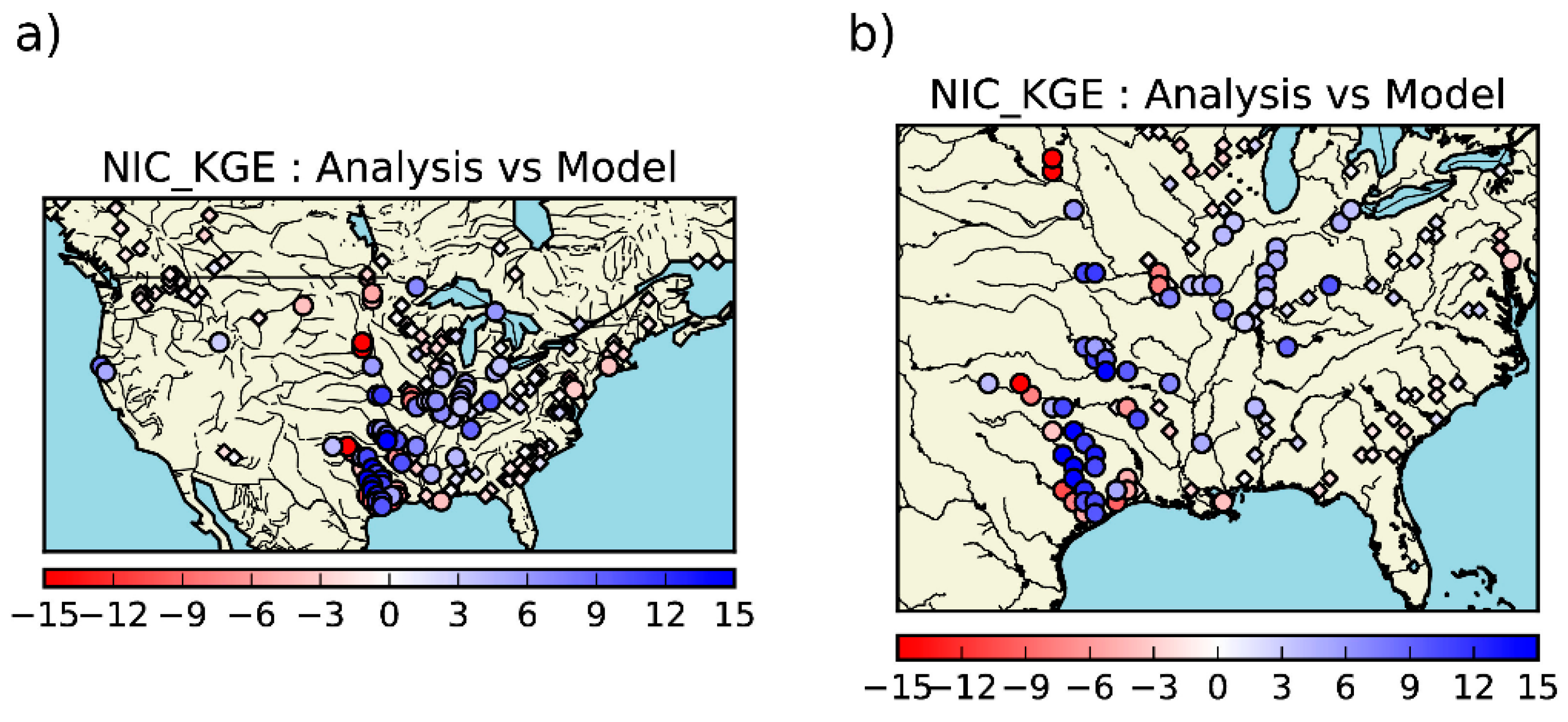
The statistical scores for surface soil moisture from the model and the analysis (third layer of soil between 4 and 10 cm depth) over 2010–2016 when compared with ground measurements from the USCRN network (at 5 cm depth) are presented in

Table 3. Analysis impact evaluation against in situ measurements of soil moisture from the US Climate Reference Network (USCRN) network. In situ measurements at a depth of 5 cm are used to evaluate soil moisture from the third layer of soil (4–10 cm) from either the model or analysis experiment over 2010–2016. The normalized information contribution (NIC) is applied to the correlation (anomaly correlations) values. NIC scores are classified according to three categories: (i) negative impact from the analysis with respect to the model with values smaller than −3%, (ii) positive impact from the analysis with respect to the model with values greater than +3%, and (iii) neutral impact from the analysis with respect to the model with values between −3% and 3%.

110 (110) Stations with Significant R (Anomaly R)	Median R (Anomaly R)	Median ubRMSD	Positive Impact: >+3	←3 Negative Impact: <−3	Neutral Impact [−3; +3]
Model	0.72 ± 0.02 * (0.60 ± 0.02 *)	0.049 ± 0.004 *	N/A	N/A	N/A
Analysis	0.74 ± 0.02 * (0.60 ± 0.02 *)	0.048 ± 0.004 *	46% (18%)	8% (1%)	46% (81%)

* 95% confidence interval of the median derived from a 10,000 samples bootstrapping.

. Median R values on volumetric soil moisture time-series (anomaly time series), along with their 95% confidence interval of the median, derived from 10,000-sample bootstrapping are as follows: 0.72 ± 0.02 (0.60 ± 0.02) and 0.74 ± 0.02 (0.60 ± 0.02), while median ubRMSDs are 0.049 ± 0.004 and 0.048 ± 0.004 for the model and the analysis, respectively. Figure 7a,b illustrate correlation values on volumetric and anomaly time-series between the model and the observations, respectively, for each station. Figure 7c,d represent the added value of the analysis expressed through the NIC index (Equation (1)) applied for correlations (NIC_R) values on volumetric and anomaly time-series; large blue circles represent a positive impact from the analysis at NIC_R greater that +3 (i.e., R values are better when the analysis is used than when the model is used), large red circles a degradation from the analysis at NIC_R smaller than −3, while diamond symbols represent a rather neutral impact at NIC_R in between [−3; +3]. While 46% (81%) of the pool of stations present a rather neutral impact for R values on volumetric (anomaly) time series, stations more impacted by the analysis tend to be positively impacted at 46% (18%), to be compared with 8% (1%) of negative impacts. Although differences between the model run and the analysis are rather small, these results underline the added value of the analysis with respect to the model run.

3.2.3. Streamflow

A subset of 258 out of 531 gauging stations was selected for the evaluation according to the criteria described in the methodology section, with KGE scores within the [0, 1] interval. Figure 8 presents the performance of analysed streamflow with respect to the one from the model run for this pool of stations, with a focus on the eastern part of the domain. NIC_KGE values are presented following the same classification as NIC_R applied to soil moisture. Scores are presented in

Table 4. Analysis impact evaluation against daily streamflow over 2010–2016. The impact from the analysis with respect to the model is assessed through the normalized information contribution (NIC) applied to the Kling–Gupta efficiency (KGE) score, as well as using normalized relative error of simulated or analysed mean (RE_μ) and standard deviation (RE_σ). Scores are classified according to three categories: (i) negative impact from the analysis with respect to the model with values smaller than −3, (ii) positive impact from the analysis with respect to the model with values greater than +3, and (iii) neutral impact from the analysis with respect to the model with values between −3 and 3.

258 out of 531 Stations with KGE Greater than 0	Positive Impact: >+3	Negative Impact: <−3	Neutral Impact [−3; +3]
NICKGE	26%	12%	62%
NREσ	22%	1%	77%
NREμ	34%	1%	65%

. Looking at NIC_KGE, 62% of the pool of stations (258 stations) present a rather neutral impact (at NIC_KGE between [−3; 3]) and 26% of the stations present a positive impact (at NIC_KGE > +3), while only 12% of stations have a negative impact (at NIC_KGE < −3). NICR, N_REσ, and N_REμ follow the same classification (with even a smaller percentage of stations being negatively affected by the analysis; 1%); when the analysis is impacting streamflow representation, it tends to be a positive impact.

4. Potential Applications, Discussions, and Perspectives

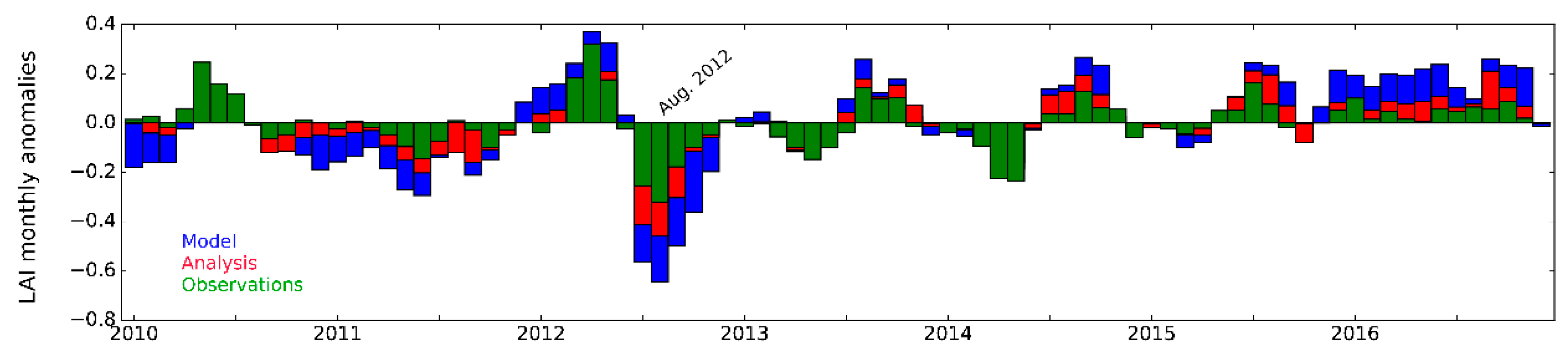
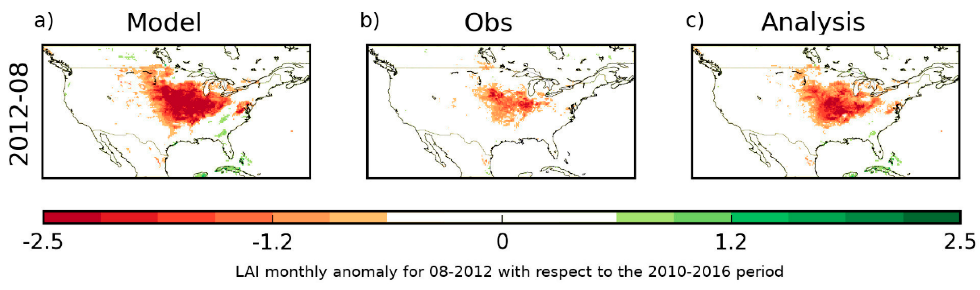
4.1. Could LDAS-Monde be Used to Monitor Agricultural Droughts?

The previous section has highlighted the LDAS-Monde ability to enhance the monitoring accuracy for land surface variables. It should then be possible to use it to better represent extreme events like agricultural droughts. Figure 9 represents monthly LAI anomalies averaged over the U.S. corn belt (simplified as a box from 110°W to 70°W and 30°N to 50°N) with respect to 2010–2016 means from the model, the analysis, and the observations. As shown by Figure 9, for the second part of the year 2012, LAI observations exhibit a strong negative anomaly at this domain scale. While it is also visible in the model, the latter clearly overestimates the intensity of the observed anomaly. The analysed LAI anomaly is closer to the observed one than the model. This extreme drought event is known as the August 2012 U.S. corn belt drought. The U.S. Department of Agriculture (USDA, www.nass.usda.gov, last access June 2018) estimated that corn yield (per acre of planted crop) was 26% below the expectation that they had at the beginning of the 2012 growing season. The 2012 corn yield deficit and the implied climatic impact was classified as a ‘historic event’ [54]. As visible on Figure 9, spring 2012 presents a positive anomaly for vegetation. Ref. [55] defined spring 2012 as the earliest false spring in the North American record (i.e., a period of weather in late winter or early spring allowing vegetation to be prematurely brought out of dormancy). This false spring has contributed to an earlier dry out of the soil. Figure 10 presents maps of the LAI anomaly for this specific month for the model, observations, and analysis from left to right, respectively. Compared with the observations (Figure 10b), the area affected by the anomaly in the model (Figure 10a) is too large and too intense, while the analysis (Figure 10c) better matches the observed pattern in both space and intensity. This impact is valid when compared with most of the severe droughts events that occurred over CONUS (data from the National Oceanic and Atmospheric Administration (NOAA) state of the climate website, last access April 2018 https://www.ncdc.noaa.gov/sotc/drought/201803, not shown). Hence, LDAS-Monde provides a better tool than the model alone to monitor extreme events like agricultural droughts.

It is also worth mentioning that if LDAS-Monde brings a clear improvement in the representation of LAI, reducing the overestimation duration as well as the minimal values, as its model counterpart, it fails capturing the observed LAI peak intensity. Ref. [13] has evaluated the model sensitivity of the observation for Europe over 2000–2012 reflected in the SEKF Jacobians. The Jacobians depend on the model physics and their examination provides useful insight that explains the data assimilation system performances [21,56]. Ref. [13] suggests a seasonal dependency of the model sensitivity to the observed LAI. High sensitivity is found in autumn. Smaller model sensitivity at the time of the year where the peak LAI occurs (late spring) prevails the analysis to match the observations correctly.

As highlighted by [57], who have evaluated the capacity of several LSMs (including ISBA) to accurately simulate observed energy and water fluxes during droughts, there is a need to re-examine existing model components in LSMs to improve simulations of soil hydrological processes and water–plant interactions. It appears from Figure 2 that although the analysis is able to correct the overestimated LAI values in winter, the minimum LAI thresholds used in ISBA has to be revisited. Recently, the satellite derived LAI data have been disaggregated following a Kalman filtering technique developed by [58]. This enables the LAI signal for each vegetation type to be separated within the pixel, which provides a dynamic vegetation-dependent estimate of the assimilated LAI within the pixel [59]. This new dataset will make it possible to modify the minimum LAI thresholds accordingly.

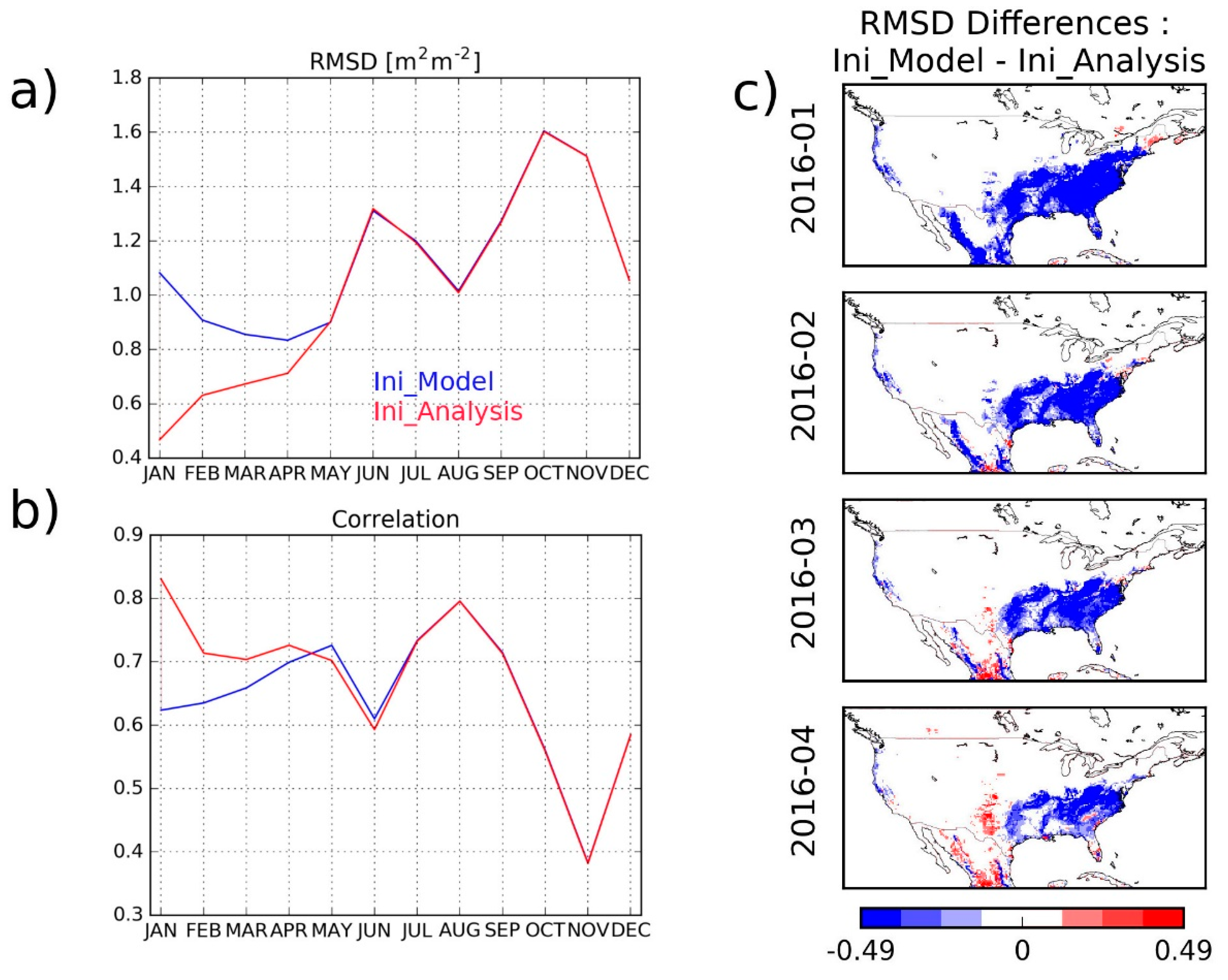
4.2. Could LDAS-Monde Provide Accurate Initial Conditions for Vegetation Forecasts?

In the context of NWP, assimilation of satellite observations in atmospheric models has the capacity to mitigate model deficiencies, leading to better estimates of system states. This has been the main driver of the improvement of both weather forecast skill and lead time [60]. Data assimilation is able to produce similar benefits for LSVs forecasting. Seeking to foster a link with applications, LDAS-Monde could not only be used to monitor the LSVs, but could also be integrated into a forecasting system (at different time scales) assuming that it can provide better initial conditions than a model run and that its impact lasts in time. Many applications could benefit from a better representation of the LSVs, from NWP [61], to early warning systems of, for example, agricultural drought and yield forecasts. As a first step towards such early warning systems, Figure 11 shows a comparison between LAI from the two last simulations presented in Table 1: Ini_Model and Ini_Analysis. Figure 11a,b shows monthly RMSD (R) values for the year 2016 for LAI. A strong impact is visible not only from the beginning of the two simulations, but also a few months later (up to April). The four maps of Figure 11c show RMSD differences between Ini_analysis and Ini_model from January to April. All maps are dominated by negative values (in blue), suggesting that Ini_analysis presents a better match with the observed LAI and that analysis effects last in time. Southeastern part of the domain is mainly affected, these areas are dominated by broadleaves forest as well as C3 crops. Large differences between the model and the analysis during winter time (as shown on Figure 2) suggest that the minimum LAI threshold used in the model for these vegetation types has to be revisited. Such results are strongly linked to the time of the year when the simulation is initialised by the analysis, that is, the greater the prior difference between the model and the analysis experiments will be, the stronger the impact. As for LAI, and according to Figure 2a, marked impact would be expected from July to March. It is also very promising that the impact of LAI initialisation lasts in time for several weeks or even months. Those results are in line with findings from [5] who have assimilated biomass and LAI observations at “site-level” in CLM4.5. They found that monthly forecasts (and even longer forecasts range) were improved by data assimilation compared with forecasts without data assimilation.

Although the ISBA LSM does not directly represent grain yield (GY), it is assumed that the regional-scale simulations of above-ground biomass from a generic LSM can provide the inter-annual variability as a proxy for GY [62,63]. Refs. [13,64] have also found that the LDAS-Monde analysed above-ground biomass inter-annual variability was in better agreement with that of GY than its open-loop counterpart. These studies have been performed over France using straw cereal GY values from the Agreste French agricultural statistics portal (http://agreste.agriculture.gouv.fr). If more evaluations are required to assess LDAS-Monde capacity to represent GY, it paves the way towards potential productivity and yield forecasting system.

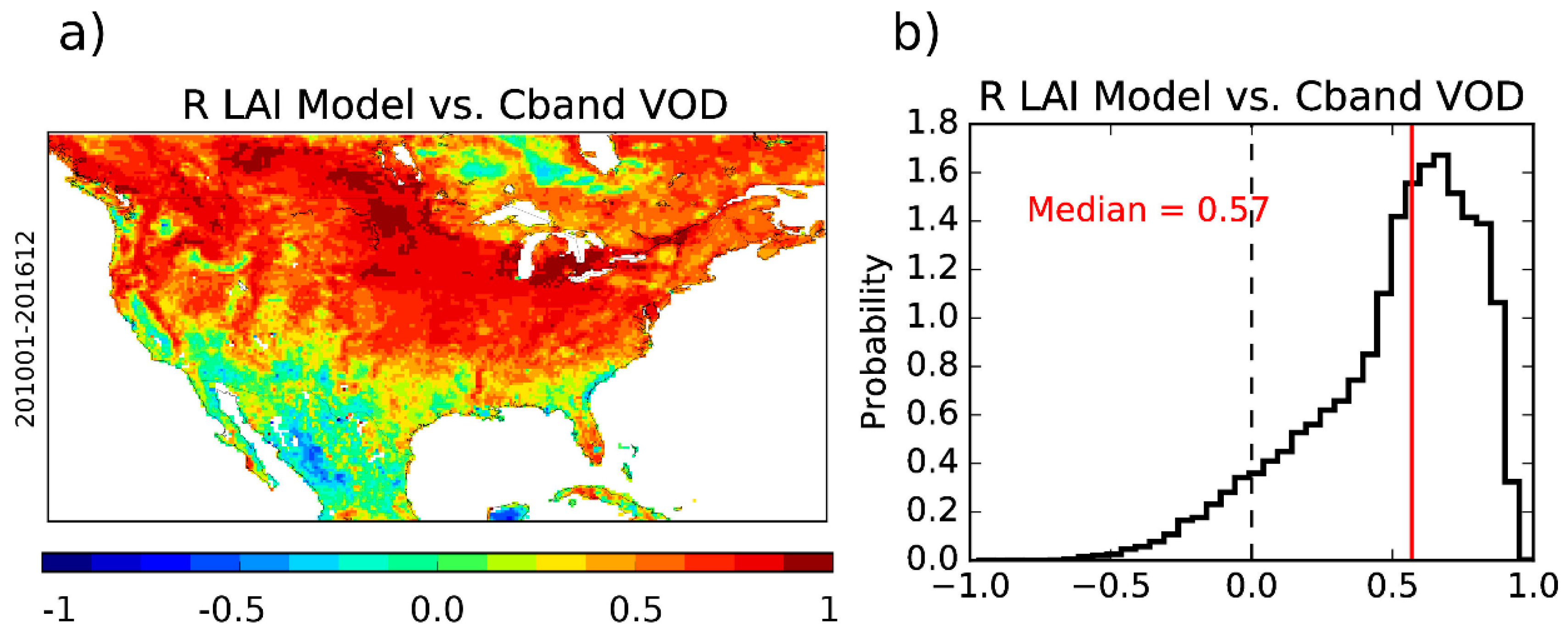
4.3. Which Alternative Data to Better Constrain LDAS-Monde?

LDAS-Monde re-analyses presented above were repeated, assimilating only SSM or LAI, the results suggested that most of the skill came from the assimilation of LAI (not shown). Assimilating LAI permits to analyze not only LAI itself, but also the root zone soil moisture. While assimilating SSM does mainly affect the first layers of soil (layer 2, 1 cm to 4 cm and layer 3, 4 cm to 10 cm), assimilating LAI has an impact on deeper layers (up to 60 cm) and is more efficient to analyse the root zone soil moisture too. This has also been suggested by [13], when analysing the ISBA LSM sensitivity to the assimilated observations through the SEKF Jacobians.

However, the LAI product used in this study is available every 10 days at best, making it less efficient to constrain the ISBA LSM, particularly in areas of the world affected by clouds for long periods of time (e.g., areas affected by the monsoon regime). Another caveat is the use of a single LAI value for all vegetation types that are represented in SURFEX. As detailed in [20], the innovation is computed from the difference between the observed LAI and the modelled LAI aggregated over all the vegetation types. Then, the Kalman gain is calculated for each individual vegetation type. The analysis increment is added to the background for each vegetation type, producing a vegetation-dependent analysis update. The vegetation dependence is introduced in the Kalman gain via the Jacobian elements. As mentioned already, the possibility of having LAI estimates for each type of vegetation is under investigation [59] and has the capacity of overcoming the above-mentioned weakness. An extension of this work is under development to assimilate in LDAS-Monde the disaggregated LAI product for each vegetation type independently, with very promising preliminary results [65].

Microwave remote sensing over land has mainly focused on soil moisture retrieval [66,67] and vegetation was mostly considered during the retrieval of surface soil moisture as a by-pass product affecting the signal penetration to the surface [68,69]. The attenuation of the signal (i.e., when passing through the vegetation) depends on the vegetation optical depth (VOD). VOD describes the attenuation of radiation due to scattering and absorption within the vegetation layer, which is caused by the water contained in the vegetation. It is function of the frequency of the microwave sensor, the water content of the plant (trunk, branches, leaves), as well as the biomass (e.g., [70,71,72,73]. VOD can be retrieved from microwave data, for example, from the L-band soil moisture and ocean salinity (SMOS) mission [74] or the C-band advanced scatterometer (ASCAT) mission on-board the meteorological operational satellite A (MetOp-A) [75,76]. VOD can be related to LAI (e.g., [77,78,79,80]. Figure 12 presents a map of temporal correlation coefficient values between modelled LAI and microwave-derived VOD from radar backscatter measurements of ASCAT [75,76] (Figure 12a), as well as their distribution (Figure 12b) for 2010–2016. High correlations values are found in large parts of the domain, with a median value of 0.57. The northern part of the domain shows R values greater than 0.7, while smaller R values (and even negative R values) are found in the southern part of the domain. Over dry soils, sub-surface scattering from the microwave signal potentially affects the VOD estimates (Wolfgang Wagner, TU WIEN, personal communication, April 2018). The same VOD dataset has a higher median R value with the observed LAI, that is, 0.88. Consequently it better correlates with the analysis (median R values of 0.61) than with the model. If a strong statistical relationship between C-band VOD and LAI can be obtained through the use of, for example, machine learning techniques (like neural network techniques, [81], it could enable obtaining a surrogate of LAI based on C-band VOD that would have the advantage of having higher temporal frequency than the current LAI product (low frequency microwave observations are not affected much by clouds and are not affected by solar elevation). Such a product could then be assimilated into LDAS-Monde to better constrain the system. Looking at such a relationship for data assimilation purposes is currently under study at CNRM.

Also, retrieved soil moisture is assimilated in LDAS-Monde, from active radar backscatter (σ_o) observations. Retrieval methods usually make use of land surface parameters and auxiliary information (like vegetation, texture, and temperature), possibly being inconsistent with specific model simulations (which also include these parameters, but potentially from different sources). Also, if retrievals and model simulations rely on similar types of auxiliary information, their errors may be cross-correlated, potentially degrading the system performance [82]. This leads to an increasing tendency towards the direct assimilation of σ_o observations (and of passive radiometer brightness temperature, T_b, as well) [83,84,85,86,87]. CNRM is also investigating the direct assimilation of σ_o. It requires the implementation of a forward model for σ_o in the ISBA LSM. Ref. [85] used the Water Cloud Model [88] to relate surface soil moisture from the Global Land Evaporation Amsterdam Model (GLEAM, [45,89]) to σ_o for data assimilation purposes. Within LDAS-Monde, both surface soil moisture and leaf area index could be related to the radar backscatter.

5. Conclusions

In this study, LDAS-Monde sequential assimilation of satellite derived surface soil moisture and leaf area index, forced by ERA-5 latest atmospheric re-analysis, was applied to the CONtiguous US domain. Ref. [28] have highlighted the added value of using the ERA-5 atmospheric reanalysis to force the ISBA Land Surface Model over the CONtiguous US for the 2010–2016 period. They found that the use of ERA-5 instead of ERA-interim leads to significant improvements in the representation of the land surface variables linked to the terrestrial water cycle (e.g., surface soil moisture, river discharges, snow depth, and turbulent fluxes), but to a rather neutral impact on land surface variables linked to the vegetation cycle (e.g., evapotranspiration, carbon uptake, and leaf area index). Assimilating satellite derived observations linked to vegetation (LAI in this application) through LDAS-Monde forced by ERA-5 not only leads to a clear improvement in the representation of the vegetation cycle in ISBA, but brings further improvement on the representation of the terrestrial water cycle. The results have highlighted the stronger impact of LAI observations assimilation with respect to soil moisture assimilation. Other vegetation-related observations such as vegetation optical depth could be used, under specific circumstances, as a surrogate of LAI limiting the negative impact of the rather low temporal frequency of the LAI product. LDAS-Monde is a powerful tool to track the evolution of land surface variables and to monitor extreme events such as agricultural drought. Since LDAS-Monde analysis is more accurate than a simple model run, it can be used to initialise a forecast experiment of the land surface variables. Preliminary results suggest that its impact on forecast experiments, in particular with respect to vegetation, is positive and lasts in time. It opens the way towards applications from monitoring to forecasting land surface states. For that purpose, LDAS-Monde will be forced by other, higher spatial resolution, ECMWF atmospheric products like the high resolution forecast (HRES, current spatial resolution of ~9 km), which also gives daily forecasts up to 10 days ahead and/or the ensemble forecast (ENS, current spatial resolution of ~18 km), giving daily forecasts up to 15 days (46 days twice a week).

References

1. Dirmeyer, P.A.; Gao, X.; Zhao, M.; Guo, Z.; Oki, T.; Hanasaki, N. The Second Global Soil Wetness Project (GSWP-2): Multi-model analysis and implications for our perception of the land surface. Bull. Am. Meteorol. Soc. 2006, 87, 1381–1397. [Google Scholar] [CrossRef]
2. Schellekens, J.; Dutra, E.; Martínez-de la Torre, A.; Balsamo, G.; van Dijk, A.; Sperna Weiland, F.; Minvielle, M.; Calvet, J.-C.; Decharme, B.; Eisner, S.; et al. A global water resources ensemble of hydrological models: The eartH2Observe Tier-1 dataset. Earth Syst. Sci. Data 2017, 9, 389–413. [Google Scholar] [CrossRef]
3. Lettenmaier, D.P.; Alsdorf, D.; Dozier, J.; Huffman, G.J.; Pan, M.; Wood, E.F. Inroads of remote sensing into hydrologic science during the WRR era. Water Resour. Res. 2015, 51, 7309–7342. [Google Scholar] [CrossRef] [Green Version]
4. Reichle, R.H.; Koster, R.D.; Liu, P.; Mahanama, S.P.; Njoku, E.G.; Owe, M. Comparison and assimilation of global soil moisture retrievals from the Advanced Microwave Scanning Radiometer for the Earth Observing System (AMSR-E) and the Scanning Multichannel Microwave Radiometer (SMMR). J. Geophys. Res. 2007, 112, D09108. [Google Scholar] [CrossRef]
5. Fox, A.M.; Hoar, T.J.; Anderson, J.L.; Arellano, A.F.; Smith, W.K.; Litvak, M.E.; MacBean, N.; Schimel, D.S.; Moore, D.J.P. Evaluation of a Data Assimilation System for Land Surface Models using CLM4.5. J. Adv. Model. Earth Syst. 2018. [Google Scholar] [CrossRef]
6. Sawada, Y.; Koike, T. Simultaneous estimation of both hydrological and ecological parameters in an ecohydrological model by assimilating microwave signal. J. Geophys. Res. Atmos. 2014, 119. [Google Scholar] [CrossRef]
7. Sawada, Y.; Koike, T.; Walker, J.P. A land data assimilation system for simultaneous simulation of soil moisture and vegetation dynamics. J. Geophys. Res. Atmos. 2015, 120. [Google Scholar] [CrossRef]
8. McNally, A.; Arsenault, K.; Kumar, S.; Shukla, S.; Peterson, P.; Wang, S.; Funk, C.; Peters-Lidard, C.D.; Verdin, J.P. A land data assimilation system for sub-Saharan Africa food and water security applications. Sci. Data 2017, 4, 170012. [Google Scholar] [CrossRef] [PubMed] [Green Version]
9. Mitchell, K.E.; Lohmann, D.; Houser, P.R.; Wood, E.F.; Schaake, J.C.; Robock, A.; Cosgrove, B.A.; Sheffield, J.; Duan, Q.; Luo, L.; et al. The multi-institution North American Land Data Assimilation System (NLDAS): Utilizing multiple GCIP products and partners in a continental distributed hydrological modeling system. J. Geophys. Res. 2004, 109, D07S90. [Google Scholar] [CrossRef]
10. Xia, Y.; Mitchell, K.; Ek, M.; Sheffield, J.; Cosgrove, B.; Wood, E.; Luo, L.; Alonge, C.; Wei, H.; Meng, J.; et al. Continental-scale water and energy flux analysis and validation for the North American Land Data Assimilation System project phase 2 (NLDAS-2): 1. Intercomparison and application of model products. J. Geophys. Res. 2012, 117, D03109. [Google Scholar] [CrossRef]
11. Kumar, S.V.; Jasinski, M.; Mocko, D.; Rodell, M.; Borak, J.; Li, B.; Kato Beaudoing, H.I.R.O.K.O.; Peters-Lidard, C.D. NCA-LDAS land analysis: Development and performance of a multisensor, multivariate land data assimilation system for the National Climate Assessment. J. Hydrometeorol. 2018. [Google Scholar] [CrossRef]
12. Rodell, M.; Houser, P.R.; Jambor, U.E.; Gottschalck, J.; Mitchell, K.; Meng, C.J.; Arsenault, K.; Cosgrove, B.; Radakovich, J.; Bosilovich, M.; et al. The Global Land Data Assimilation System. Bull. Am. Meteorol. Soc. 2004, 85, 381–394. [Google Scholar] [CrossRef] [Green Version]
13. Albergel, C.; Munier, S.; Leroux, D.J.; Dewaele, H.; Fairbairn, D.; Barbu, A.L.; Gelati, E.; Dorigo, W.; Faroux, S.; Meurey, C.; et al. Sequential assimilation of satellite-derived vegetation and soil moisture products using SURFEX_v8.0: LDAS-Monde assessment over the Euro-Mediterranean area. Geosci. Model Dev. 2017, 10, 3889–3912. [Google Scholar] [CrossRef] [Green Version]
14. Noilhan, J.; Mahfouf, J.-F. The ISBA land surface parameterisation scheme. Glob. Planet. Chang. 1996, 13, 145–159. [Google Scholar] [CrossRef]
15. Calvet, J.-C.; Noilhan, J.; Roujean, J.-L.; Bessemoulin, P.; Cabelguenne, M.; Olioso, A.; Wigneron, J.-P. An interactive vegetation SVAT model tested against data from six 780 contrasting sites. Agric. For. Meteorol. 1998, 92, 73–95. [Google Scholar] [CrossRef]
16. Calvet, J.-C.; Rivalland, V.; Picon-Cochard, C.; Guehl, J.-M. Modelling forest transpiration and CO2 fluxes—Response to soil moisture stress. Agric. For. Meteorol. 2004, 124, 143–156. [Google Scholar] [CrossRef]
17. Gibelin, A.-L.; Calvet, J.-C.; Roujean, J.-L.; Jarlan, L.; Los, S.O. Ability of the land surface model ISBA-A-gs to simulate leaf area index at global scale: Comparison with satellite products. J. Geophys. Res. 2006, 111, 1–16. [Google Scholar] [CrossRef]
18. Masson, V.; Le Moigne, P.; Martin, E.; Faroux, S.; Alias, A.; Alkama, R.; Belamari, S.; Barbu, A.; Boone, A.; Bouyssel, F.; et al. The SURFEXv7.2 land and ocean surface platform for coupled or offline simulation of earth surface variables and fluxes. Geosci. Model Dev. 2013, 6, 929–960. [Google Scholar] [CrossRef] [Green Version]
19. Barbu, A.L.; Calvet, J.-C.; Mahfouf, J.-F.; Albergel, C.; Lafont, S. Assimilation of Soil Wetness Index and Leaf Area Index into the ISBA-A-gs land surface model: Grassland case study. Biogeosciences 2011, 8, 1971–1986. [Google Scholar] [CrossRef] [Green Version]
20. Barbu, A.L.; Calvet, J.C.; Mahfouf, J.F.; Lafont, S. Integrating ASCAT surface soil moisture and GEOV1 leaf area index into the SURFEX modelling platform: A land data assimilation application over France. Hydrol. Earth Syst. Sci. 2014, 18, 173–192. [Google Scholar] [CrossRef] [Green Version]
21. Fairbairn, D.; Barbu, A.L.; Napoly, A.; Albergel, C.; Mahfouf, J.-F.; Calvet, J.-C. The effect of satellite-derived surface soil moisture and leaf area index land data assimilation on streamflow simulations over France. Hydrol. Earth Syst. Sci. 2017, 21, 2015–2033. [Google Scholar] [CrossRef]
22. Liu, Y.Y.; Parinussa, R.M.; Dorigo, W.A.; De Jeu, R.A.; Wagner, W.; Van Dijk, A.I.; McCabe, M.F.; Evans, J.P. Developing an improved soil moisture dataset by blending passive and active microwave satellite-based retrievals. Hydrol. Earth Syst. Sci. 2011, 15, 425–436. [Google Scholar] [CrossRef] [Green Version]
23. Liu, Y.Y.; Dorigo, W.A.; Parinussa, R.M.; de Jeu, R.A.; Wagner, W.; McCabe, M.F.; Evans, J.P.; Van Dijk, A.I. Trend-preserving blending of passive and active microwave soil moisture retrievals. Remote Sens. Environ. 2012, 123, 280–297. [Google Scholar] [CrossRef]
24. Dorigo, W.A.; Gruber, A.; De Jeu, R.A.; Wagner, W.; Stacke, T.; Loew, A.; Albergel, C.; Brocca, L.; Chung, D.; Parinussa, R.M.; et al. Evaluation of the ESA CCI soil moisture product using ground-based observations. Remote Sens. Environ. 2015. [Google Scholar] [CrossRef]
25. Dorigo, W.; Wagner, W.; Albergel, C.; Albrecht, F.; Balsamo, G.; Brocca, L.; Chung, D.; Ertl, M.; Forkel, M.; Gruber, A.; et al. ESA CCI Soil Moisture for improved Earth system understanding: State-of-the art and future directions. Remote Sens. Environ. 2017. [Google Scholar] [CrossRef]
26. Weedon, G.P.; Gomes, S.; Viterbo, P.; Shuttleworth, W.J.; Blyth, E.; Österle, H.; Adam, J.C.; Bellouin, N.; Boucher, O.; Best, M. Creation of the WATCH forcing data and its use to assess global and regional reference crop evaporation over land during the twentieth century. J. Hydrometeorol. 2011, 12, 823–848. [Google Scholar] [CrossRef]
27. Weedon, G.P.; Balsamo, G.; Bellouin, N.; Gomes, S.; Best, M.J.; Viterbo, P. The WFDEI meteorological forcing data set: WATCH Forcing data methodology applied to ERA- interim reanalysis data. Water Resour. Res. 2014, 50, 7505–7514. [Google Scholar] [CrossRef]
28. Albergel, C.; Dutra, E.; Munier, S.; Calvet, J.-C.; Munoz-Sabater, J.; de Rosnay, P.; Balsamo, G. ERA-5 and ERA-Interim driven ISBA land surface model simulations: Which one performs better? Hydrol. Earth Syst. Sci. 2018, 22, 3515–3532. [Google Scholar] [CrossRef]
29. Boone, A.; Masson, V.; Meyers, T.; Noilhan, J. The influence of the inclusion of soil freezing on simulations by a soil vegetation–atmosphere transfer scheme. J. Appl. Meteorol. 2000, 39, 1544–1569. [Google Scholar] [CrossRef]
30. Decharme, B.; Martin, E.; Faroux, S. Reconciling soil thermal and hydrological lower boundary conditions in land surface models. J. Geophys. Res.-Atmos. 2013, 118, 7819–7834. [Google Scholar] [CrossRef] [Green Version]
31. Voldoire, A.; Decharme, B.; Pianezze, J.; Lebeaupin Brossier, C.; Sevault, F.; Seyfried, L.; Garnier, V.; Bielli, S.; Valcke, S.; Alias, A.; et al. SURFEX v8.0 interface with OASIS3-MCT to couple atmosphere with hydrology, ocean, waves and sea-ice models, from coastal to global scales. Geosci. Model Dev. 2017, 10, 4207–4227. [Google Scholar] [CrossRef] [Green Version]
32. Decharme, B.; Alkama, R.; Douville, H.; Becker, M.; Cazenave, A. Global evaluation of the ISBA-TRIP continental hydrologic system, Part 2: Uncertainties in river routing simulation related to flow velocity and groundwater storage. J. Hydrometeorol. 2010, 11, 601–617. [Google Scholar] [CrossRef]
33. Decharme, B.; Alkama, R.; Papa, F.; Faroux, S.; Douville, H.; Prigent, C. Global offline evaluation of the ISBA-TRIP flood model. Clim. Dynam. 2012, 38, 1389–1412. [Google Scholar] [CrossRef]
34. Vergnes, J.-P.; Decharme, B. A simple groundwater scheme in the TRIP river routing model: Global off-line evaluation against GRACE terrestrial water storage estimates and observed river discharges. Hydrol. Earth Syst. Sci. 2012, 16, 3889–3908. [Google Scholar] [CrossRef] [Green Version]
35. Vergnes, J.-P.; Decharme, B.; Habets, F. Introduction of groundwater capillary rises using subgrid spatial variability of topography into the ISBA land surface model. J. Geophys. Res.-Atmos. 2014, 119, 11065–11086. [Google Scholar] [CrossRef]
36. Leroux, D.J.; Calvet, J.-C.; Munier, S.; Albergel, C. Using Satellite-Derived Vegetation Products to Evaluate LDAS-Monde over the Euro-Mediterranean Area. Remote Sens. 2018, 10, 1199. [Google Scholar] [CrossRef]
37. Mätzler, C.; Standley, A. Relief effects for passive microwave remote sensing. Int. J. Remote Sens. 2000, 21, 2403–2412. [Google Scholar] [CrossRef]
38. Draper, C.; Mahfouf, J.-F.; Calvet, J.-C.; Martin, E.; Wagner, W. Assimilation of ASCAT near-surface soil moisture into the SIM hydrological model over France. Hydrol. Earth Syst. Sci. 2011, 15, 3829–3841. [Google Scholar] [CrossRef] [Green Version]
39. Reichle, R.H.; Koster, D. Bias reduction in short records of satellite soil moisture. Geophys. Res. Lett. 2004, 31, L19501. [Google Scholar] [CrossRef]
40. Drusch, M.; Wood, E.F.; Gao, H. Observations operators for the direct assimilation of TRMM microwave imager retrieved soil moisture. Geophys. Res. Lett. 2005, 32, L15403. [Google Scholar] [CrossRef]
41. Scipal, K.; Drusch, M.; Wagner, W. Assimilation of a ERS scatterometer derived soil moisture index in the ECMWF numerical weather prediction system. Adv. Water Resour. 2008, 31, 1101–1112. [Google Scholar] [CrossRef]
42. Boussetta, S.; Balsamo, G.; Dutra, E.; Beljaars, A.; Albergel, C. Assimilation of surface albedo and vegetation states from satellite observations and their impact on numerical weather prediction. Remote Sens. Environ. 2015, 163, 111–126. [Google Scholar] [CrossRef] [Green Version]
43. Baret, F.; Weiss, M.; Lacaze, R.; Camacho, F.; Makhmared, H.; Pacholczyk, P.; Smetse, B. GEOV1: LAI and FAPAR essential climate variables and FCOVER global time series capitalizing over existing products, Part 1: Principles of development and production. Remote Sens. Environ. 2013, 137, 299–309. [Google Scholar] [CrossRef]
44. Hersbach, H.; Dee, D. ERA-5 Reanalysis is in Production; ECMWF Newsletter, Number 147; ECMWF: Reading, UK, 2016; p. 7. [Google Scholar]
45. Miralles, D.G.; Holmes, T.R.H.; De Jeu, R.A.M.; Gash, J.H.; Meesters, A.G.C.A.; Dolman, A.J. Global land-surface evaporation estimated from satellite-based observations. Hydrol. Earth Syst. Sci. 2011, 15, 453–469. [Google Scholar] [CrossRef] [Green Version]
46. Martens, B.; Miralles, D.G.; Lievens, H.; van der Schalie, R.; de Jeu, R.A.M.; Fernández-Prieto, D.; Beck, H.E.; Dorigo, W.A.; Verhoest, N.E.C. GLEAM v3: Satellite-based land evaporation and root-zone soil moisture. Geosci. Model Dev. 2017, 10, 1903–1925. [Google Scholar] [CrossRef]
47. Tramontana, G.; Jung, M.; Schwalm, C.R.; Ichii, K.; Camps-Valls, G.; Ráduly, B.; Reichstein, M.; Arain, M.A.; Cescatti, A.; Kiely, G.; et al. Predicting carbon dioxide and energy fluxes across global FLUXNET sites with regression algorithms. Biogeosciences 2016, 13, 4291–4313. [Google Scholar] [CrossRef] [Green Version]
48. Jung, M.; Reichstein, M.; Schwalm, C.R.; Huntingford, C.; Sitch, S.; Ahlström, A.; Arneth, A.; Camps-Valls, G.; Ciais, P.; Friedlingstein, P.; et al. Compensatory water effects link yearly global land CO2 sink changes to temperature. Nature 2017, 541, 516–520. [Google Scholar] [CrossRef] [PubMed]
49. Bell, J.E.; Palecki, M.A.; Collins, W.G.; Lawrimore, J.H.; Leeper, R.D.; Hall, M.E.; Kochendorfer, J.; Meyers, T.P.; Wilson, T.; Baker, B.; et al. U.S. Climate Reference Network soil moisture and temperature observatons. J. Hydrometeorol. 2013, 14, 977–988. [Google Scholar] [CrossRef]
50. Kumar, S.; Reichle, R.H.; Koster, R.D.; Crow, W.T.; Peters-Lidard, C. Role of Subsurface Physics in the Assimilation of Surface Soil Moisture Observations. J. Hydrometeor. 2009, 10, 1534–1547. [Google Scholar] [CrossRef] [Green Version]
51. Gupta, H.V.; Kling, H.; Yilmaz, K.K.; Martinez, G.F. Decomposition of the mean squared error and NSE performance criteria: Implications for improving hydrological modelling. J. Hydrol. 2009, 377, 80–91. [Google Scholar] [CrossRef] [Green Version]
52. Beck, H.E.; Pan, M.; Roy, T.; Weedon, G.P.; Pappenberger, F.; van Dijk, A.I.J.M.; Huffman, G.J.; Adler, R.F.; Wood, E.F. Daily evaluation of 26 precipitation datasets using Stage-IV gauge-radar data for the CONUS, Hydrol. Earth Syst. Sci. Discuss. 2018. [Google Scholar] [CrossRef]
53. Olive, W.W.; Chleborad, A.F.; Frahme, C.W.; Schlocker, J.; Schneider, R.R.; Schuster, R.L. Swelling Clays Map of the Conterminous United States; USGS: Reston, VA, USA, 1989.
54. Hoerling, M.; Eischeid, J.; Kumar, A.; Leung, R.; Mariotti, A.; Mo, K.; Schubert, S.; Seager, R. Causes and Predictability of the 2012 Great Plains Drought. Bull. Am. Meteorol. Soc. 2014, 95, 269–282. [Google Scholar] [CrossRef]
55. Ault, T.R.; Henebry, G.M.; De Beurs, K.M.; Schwartz, M.D.; Betancourt, J.L.; Moore, D. The False Spring of 2012, Earliest in North American Record. EOS 2013, 94, 181–182. [Google Scholar] [CrossRef] [Green Version]
56. Rüdiger, C.; Albergel, C.; Mahfouf, J.-F.; Calvet, J.-C.; Walker, J.P. Evaluation of Jacobians for Leaf Area Index data assimilation with an extended Kalman filter. J. Geophys. Res. 2010, 115, D09111. [Google Scholar] [CrossRef]
57. Ukkola, A.M.; De Kauwe, M.G.; Pitman, A.J.; Best, M.J.; Abramowitz, G.; Haverd, V.; Decker, M.; Haughton, N. Land surface models systematically overestimate the intensity, duration and magnitude of seasonal-scale evaporative droughts. Environ. Res. Lett. 2016, 11, 104012. [Google Scholar] [CrossRef] [Green Version]
58. Carrer, D.; Meurey, C.; Ceamanos, X.; Roujean, J.-L.; Calvet, J.-C.; Liu, S. Dynamic mapping of snow-free vegetation and bare soil albedos at global 1 km scale from 10 year analysis of MODIS satellite products. Remote Sens. Environ. 2014, 140, 420–432. [Google Scholar] [CrossRef]
59. Munier, S.; Carrer, D.; Planque, C.; Camacho, F.; Albergel, C.; Calvet, J.-C. Satellite Leaf Area Index: Global Scale Analysis of the Tendencies Per Vegetation Type Over the Last 17 Years. Remote Sens. 2018, 10, 424. [Google Scholar] [CrossRef]
60. Bauer, P.; Thorpe, A.; Brunet, G. The quiet revolution of numerical weather prediction. Nature 2015, 525, 47–55. [Google Scholar] [CrossRef] [PubMed]
61. De Rosnay, P.; Drusch, M.; Vasiljevic, D.; Balsamo, G.; Albergel, C.; Isaksen, L. A simplified extended Kalman filter for the global operational soil moisture analysis at ECMWF. Q. J. R. Meteorol. Soc. 2013, 139, 1199–1213. [Google Scholar] [CrossRef]
62. Calvet, J.-C.; Lafont, S.; Cloppet, E.; Souverain, F.; Badeau, V.; Le Bas, C. Use of agricultural statistics to verify the interannual variability in land surface models: A case study over France with ISBA-A-gs. Geosci. Model Dev. 2012, 5, 37–54. [Google Scholar] [CrossRef]
63. Canal, N.; Calvet, J.-C.; Decharme, B.; Carrer, D.; Lafont, S.; Pigeon, G. Evaluation of root water uptake in the ISBA-A-gs land surface model using agricultural yield statistics over France. Hydrol. Earth Syst. Sci. 2014, 18, 4979–4999. [Google Scholar] [CrossRef]
64. Dewaele, H.; Munier, S.; Albergel, C.; Planque, C.; Laanaia, N.; Carrer, D.; Calvet, J.-C. Parameter optimisation for a better representation of drought by LSMs: Inverse modelling vs. sequential data assimilation. Hydrol. Earth Syst. Sci. 2017, 21, 4861–4878. [Google Scholar] [CrossRef]
65. Munier, S.; Leroux, D.; Albergel, C.; Carrer, D.; Calvet, J.C. Hydrological impacts of the assimilation of satellite-derived disaggregated Leaf Area Index into the SURFEX modelling platform. Hydrol. Earth Syst. Sci. Discuss. 2018. in preparation. [Google Scholar]
66. Entekhabi, D.; Nakamura, H.; Njoku, E.G. Solving the inverse problem for soil moisture and tem-perature profiles by the sequential assimilation of multifrequency remotely sensed observations. IEEE Trans. Geosci. Remote Sens. 1994, 32, 438–448. [Google Scholar] [CrossRef]
67. Reichle, R.H.; Entekhabi, D.; McLaughlin, D.B. Downscaling of radio brightness measurements for soil moisture estimation: A four-dimensional variational data assimilation approach. Water Resour. Res. 2001, 37, 2353–2364. [Google Scholar] [CrossRef] [Green Version]
68. Kurum, M.; Lang, R.H.; O’Neill, P.E.; Joseph, A.T.; Jackson, T.J.; Cosh, M. A first-order radiative transfer model for microwave radiometry of forest canopies at L-band. IEEE Trans. Geosci. Remote Sens. 2011, 49, 3167–3179. [Google Scholar] [CrossRef]
69. Kurum, M.; O’Neill, P.E.; Lang, R.H.; Joseph, A.T.; Cosh, M.H.; Jackson, T.J. Effective tree scattering and opacity at L-band. Remote Sens. Environ. 2012, 118, 1–9. [Google Scholar] [CrossRef] [Green Version]
70. Meesters, A.G.C.A.; Jeu, R.A.M.D.; Owe, M. Analytical derivation of the vegetation optical depth from the microwave polarization difference index. IEEE Geosci. Remote Sens. Lett. 2005, 2, 121–123. [Google Scholar] [CrossRef]
71. Liu, Y.Y.; Jeu, R.D.; McCabe, M.F.; Evans, J.P.; van Dijk, A.I.J.M. Global lon-term passive microwave satellite-based retrievals of vegetation optical depth. Geophys. Res. Lett. 2011, 38. [Google Scholar] [CrossRef]
72. Konings, A.G.; Gentine, P. Global variations in ecosystem-scale isohydricity. Glob. Chang. Biol. 2016, 23, 891–905. [Google Scholar] [CrossRef] [PubMed]
73. Tian, F.; Brandt, M.; Liu, Y.Y.; Verger, A.; Tagesson, T.; Diouf, A.A.; Rasmussen, K.; Mbow, C.; Wang, Y.; Fensholt, R. Remote sensing of vegetation dynamics in drylands: Evaluating vegetation optical depth (VOD) using AVHRR NDVI and in situ green biomass data over West African Sahel. Remote Sens. Environ. 2016, 177, 265–276. [Google Scholar] [CrossRef] [Green Version]
74. Fernandez-Moran, R.; Wigneron, J.-P.; De Lannoy, G.; Lopez-Baeza, E.; Parrens, M.; Mialon, A.; Mahmoodi, A.; Al-Yaari, A.; Bircher, S.; Al Bitar, A.; et al. A new calibration of the effective scattering albedo and soil roughness parameters in the SMOS SM retrieval algorithm. Int. J. Appl. Earth Obs. Geoinf. 2017, 62, 27–38. [Google Scholar] [CrossRef]
75. Vreugdenhil, M.; Dorigo, W.A.; Wagner, W.; de Jeu, R.A.M.; Hahn, D.; Marle, M.J.E. Analyzing the vegetation parameterization in the TU-Wien ASCAT soil moisture retrieval. IEEE Trans. Geosci. Remote Sens. 2016, 54, 3513–3531. [Google Scholar] [CrossRef]
76. Vreugdenhil, M.; Hahn, S.; Melzer, T.; Bauer-Marschallinger, B.; Reimer, C.; Dorigo, W.A.; Wagner, W. Assessing vegetation dynamics over Mainland Australia with Metop ASCAT. IEEE J. Sel. Top. Appl. Earth Obs. Remote Sens. 2016, 10, 2240–2248. [Google Scholar] [CrossRef]
77. Zribi, M.; Chahbi, A.; Shabou, M.; Lili-Chabaane, Z.; Duchemin, B.; Baghdadi, N.; Amri, R.; Chehbouni, A. Soil surface moisture estimation over a semi-arid region using ENVISAT ASAR radar data for soil evaporation evaluation. Hydrol. Earth Syst. Sci. Discuss. 2011, 15, 345–358. [Google Scholar] [CrossRef] [Green Version]
78. Kim, Y.; Jackson, T.; Bindlish, R.; Lee, H.; Hong, S. Radar Vegetation Index for Estimating the Vegetation Water Content of Rice and Soybean. IEEE Geosci. Remote Sens. Lett. 2012, 9, 564–568. [Google Scholar] [CrossRef]
79. Sawada, Y.; Tsutsui, H.; Koike, T.; Rasmy, M.; Seto, R.; Fuji, H. A Field Verification of an Algorithm for Retrieving Vegetation Water Content from Passive Microwave Observations. IEEE Trans. Geosci. Remote Sens. 2016, 54, 2082–2095. [Google Scholar] [CrossRef]
80. Momen, M.; Wood, J.D.; Novick, K.A.; Pangle, R.; Pockman, W.T.; McDowell, N.G.; Konings, A.G. Interacting effects of leaf water potential and biomass on vegetation optical depth. J. Geophys. Res. Biogeosci. 2017, 122, 3031–3046. [Google Scholar] [CrossRef]
81. Rodríguez-Fernández, N.J.; Muñoz Sabater, J.; Richaume, P.; de Rosnay, P.; Kerr, Y.H.; Albergel, C.; Drusch, M.; Mecklenburg, S. SMOS near-real-time soil moisture product: Processor overview and first validation results. Hydrol. Earth Syst. Sci. 2017, 21, 5201–5216. [Google Scholar] [CrossRef]
82. De Lannoy, G.J.M.; Reichle, R.H.; Pauwels, V.R.N. Global calibration of the GEOS-5 L-band microwave radiative transfer model over nonfrozen land using SMOS observations. J. Hydrometeorol. 2013, 14, 765–785. [Google Scholar] [CrossRef]
83. De Lannoy, G.J.M.; Reichle, R.H. Global assimilation of multiangle and multipolarization SMOS brightness temperature observations into the GEOS-5 catchment Land Surface Model for soil moisture estimation. J. Hydrometeorol. 2016, 17, 669–691. [Google Scholar] [CrossRef]
84. Han, X.; Hendricks Franssen, H.-J.; Montzka, C.; Vereecken, H. Soil moisture and soil properties estimation in the community land model with synthetic brightness temperature observations. Water Resour. Res. 2014, 50, 6081–6105. [Google Scholar] [CrossRef]
85. Lievens, H.; Al Bitar, A.; Verhoest, N.E.C.; Cabot, F.; De Lannoy, G.J.M.; Drusch, M.; Dumedah, G.; Hendricks Franssen, H.J.; Kerr, Y.H.; Kumar Tomer, S.; et al. Optimization of a radiative transfer forward operator for simulating SMOS brightness temperatures over the Upper Mississippi Basin. J. Hydrometeorol. 2015, 16, 1109–1134. [Google Scholar] [CrossRef]
86. Lievens, H.; Martens, B.; Verhoest, N.E.C.; Hahn, S.; Reichle, R.H.; Miralles, D.G. Assimilation of global radar backscatter and radiometer brightness temperature observations to improve soil moisture and land evaporation estimates. Remote Sens. Environ. 2016, 189, 194–210. [Google Scholar] [CrossRef]
87. Zhao, L.; Yang, Z.-L.; Hoar, T.J. Global Soil Moisture Estimation by Assimilating AMSR-E Brightness Temperatures in a Coupled CLM4–RTM–DART System. J. Hydrometeorol. 2016, 17, 2431–2454. [Google Scholar] [CrossRef]
88. Attema, E.; Ulaby, F. Vegetation modeled as a water cloud. Radio Sci. 1978, 13, 357–364. [Google Scholar] [CrossRef]
89. Miralles, D.G.; De Jeu, R.A.M.; Gash, J.H.; Holmes, T.R.H.; Dolman, A.J. Magnitude and variability of land evaporation and its components at the global scale. Hydrol. Earth Syst. Sci. 2011, 15, 967–981. [Google Scholar] [CrossRef] [Green Version]
Figure 1. Averaged (a) surface soil moisture from the Climate Change Initiative project of ESA (for pixels with less than 15% of urban areas and with an elevation of less than 1500 m above sea level); (b) GEOV1 leaf area index from the Copernicus Global Land Service project (for pixels covered by more than 90% of vegetation) from 2010 to 2016. ESA CCI SSM—European Space Agency and Climate Change Initiative surface soil moisture; LAI—leaf area index.
Remotesensing 10 01627 g001
Figure 2. Leaf area index time series from the model (blue line), the observations (green dots and dashed line), and the analysis (red line) averaged over the whole domain from 2010 to 2017.
Remotesensing 10 01627 g002
Figure 3. Top row; leaf area index from (a) the model, (b) the observations, and (c) the analysis averaged over the 2010–2016 time period. Bottom row: seasonal (d) root mean square difference (RMSD) and (e) correlation values between leaf area index (LAI) from the model (in blue), the analysis (in red) and GEOV1 LAI estimates from the Copernicus Global Land Service project from 2010 to 2016.
Remotesensing 10 01627 g003
Figure 4. (ae) same as Figure 3 for soil moisture.
Remotesensing 10 01627 g004
Figure 5. Analysis increments averaged over the 2010–2016 time period for (a) LAI in m2 m−2, (b) second, (c) fourth, and (d) sixth layer of soil moisture in m3 m−3.
Remotesensing 10 01627 g005
Figure 6. Top row: (a) normalized root mean square difference (RMSD) (blue colours indicate an improvement) and (b) normalized information contribution (NIC) applied on correlations values (red colours indicate an improvement) for evapotranspiration from the analysis with respect to the model. Bottom row: same as top row for gross primary production. Units are percentages.
Remotesensing 10 01627 g006
Figure 7. Maps of correlation (R) on volumetric time-series (a) and anomaly time-series (b) between in situ measurements at 5 cm depth from the US Climate Reference Network (USCRN) network and soil moisture from the model (third layer of soil between 4 cm and 10 cm) from 2010 to 2016. NIC applied on R (anomaly R) values (c,d); analysis with respect to the model. NIC scores are classified according to three categories: (i) negative impact from the analysis with respect to the model with values smaller than −3% (red circles), (ii) positive impact from the analysis with respect to the model with values greater than +3% (blue circles), and (iii) neutral impact from the analysis with respect to the model with values between −3% and 3% (diamonds).
Remotesensing 10 01627 g007
Figure 8. Normalized information contribution scores based on Kling–Gupta efficiency (KGE) scores (NICKGE) (a) analysis with respect to the model, (b) zoom over the eastern part of the domain. Small diamonds represent stations for which NICKGE are between [−3; +3]. NICKGE greater than 3 (blue large circles) suggest an improvement from the analysis over the model, values smaller than −3 (red large circles) suggest a degradation. For sake of clarity, a factor of 100 has been applied to NIC.
Remotesensing 10 01627 g008
Figure 9. Leaf area index (LAI) monthly anomalies over the 2010–2016 time period for the model (blue bars), the analysis (red bars), and the CGLS GEOV1 observations (in green) over the corn belt drought defined as a box from 110°W to 70°W and 30°N to 50°N.
Remotesensing 10 01627 g009
Figure 10. (a) Monthly anomaly of leaf area index for August 2012 with respect to the 2010–2016 period, (b) same as (a) for observed leaf area index, and (c) same as (a) for analysed leaf area index.
Remotesensing 10 01627 g010
Figure 11. Seasonal (a) root mean square differences (RMSD) and (b) correlation values between observed leaf area index (LAI) and (in blue) a 12-month model run, (in red) a 12-month model run initialised by analysed conditions from LDAS-Monde. (c) RMSD differences values between a 12-month model run and a 12-month model run initialised by analysed conditions from LDAS-Monde.
Remotesensing 10 01627 g011
Figure 12. (a) Correlation coefficient values between modelled LAI and C-band vegetation optical depth (VOD) over 2010–2016, (b) probability distribution of the correlation coefficient values over the same period.
Remotesensing 10 01627 g012