Nationwide Projection of Rice Yield Using a Crop Model Integrated with Geostationary Satellite Imagery: A Case Study in South Korea


1
Department of Applied Plant Science, Chonnam National University, 77 Yongbong-ro, Buk-gu, Gwangju 61186, Korea
2
Satellite Information Center, Korea Aerospace Research Institute, 169-84 Gwahak-ro, Yuseong-gu, Daejeon 34133, Korea
*
Author to whom correspondence should be addressed.
†
Equal contribution goes to these authors.
Remote Sens. 2018, 10(10), 1665; https://doi.org/10.3390/rs10101665
Submission received: 2 September 2018
/
Revised: 16 October 2018
/
Accepted: 19 October 2018
/
Published: 21 October 2018
(This article belongs to the Section Remote Sensing in Agriculture and Vegetation)
Abstract
:The Geostationary Ocean Color Imager (GOCI) of the Communication, Ocean, and Meteorological Satellite (COMS) increases the chance of acquiring images with greater clarity eight times a day and is equipped with spectral bands suitable for monitoring crop yield in the national scale with a spatial resolution of 500 m. The objectives of this study were to classify nationwide paddy fields and to project rice (Oryza sativa) yield and production using the grid-based GRAMI-rice model and GOCI satellite products over South Korea from 2011 to 2014. Solar insolation and temperatures were obtained from COMS and the Korea local analysis and prediction systems for model inputs, respectively. The paddy fields and transplanting dates were estimated by using Moderate Resolution Imaging Spectroradiometer (MODIS) reflectance and land cover products. The crop model was calibrated using observed yield data in 11 counties and was applied to 62 counties in South Korea. The overall accuracies of the estimated paddy fields using MODIS data ranged from 89.5% to 90.2%. The simulated rice yields statistically agreed with the observed yields with mean errors of −0.07 to +0.10 ton ha−1, root-mean-square errors of 0.219 to 0.451 ton ha−1, and Nash–Sutcliffe efficiencies of 0.241 to 0.733 in four years, respectively. According to paired t-tests (α = 0.05), the simulated and observed rice yields were not significantly different. These results demonstrate the possible development of a crop information delivery system that can classify land cover, simulate crop yield, and monitor regional crop production on a national scale.
1. Introduction
Satellite-based remote sensing techniques have been applied for estimating crop yield throughout the world [1,2,3]. Advanced Very High Resolution Radiometer (AVHRR) and Moderate Resolution Imaging Spectroradiometer (MODIS) satellite imagery have been used most widely to estimate crop yield from a regional to a global scale [3,4,5]. These satellite sensors have advantages of high temporal resolution, broad coverage, and suitable multi-spectral bands to acquire crop formation. However, it is challenging to obtain invariably high-quality imagery data particularly in monsoon climate areas because of many inadequate or missing pixels caused by frequent cloud coverage during a crop growing season. For this reason, an image processing technique that retrieves the pixels contaminated by clouds is an important issue for obtaining reliable spectral information on crop conditions.
Various approaches have been applied to minimize such contaminated pixels based on image processing methods. The linear interpolation method using vegetation indices (VIs) is a traditional and straightforward technique used to retrieve the contaminated pixels by utilizing the characteristic that VI values linearly increase or decrease according to crop growth [6,7,8]. A temporal image composite method is an adequate way to reduce the cloud effects. This method selects the best possible pixels during a specific period considering atmospheric conditions and combines them into one image [3,9]. Smoothing or curve fitting methods have been applied by using various statistical algorithms based on spectral information [10,11,12]. Although all of these approaches have been proven to be practically applicable, it is difficult to ensure reliable imagery data in the case of prolonged cloudy days [13,14].
Geostationary orbit satellite sensors are primarily designed for observation and forecasting of weather conditions. These have a higher temporal resolution than Earth orbit satellite sensors such as MODIS and AVHRR due to their continuous observation characteristic in specified regions [15,16]. This characteristic can increase the chances for obtaining clear satellite imagery by acquiring many images in a single day than polar orbit satellites [14,17]. However, the imageries from these types of satellite sensors have rarely been used to estimate crop yield due to a low spatial resolution and insufficient spectral bands for monitoring crop spectral information. On the other hand, the Communication, Ocean, and Meteorological Satellite (COMS), which is one of the geostationary orbit satellites that observe the sea around the Korean Peninsula, is equipped with multi-spectral sensors that can monitor spectral crop information with a moderate spatial resolution of 500 m. The previous study compared Geostationary Ocean Color Imager (GOCI) products from COMS with MODIS images [14]. They showed that the COMS data had a more stable seasonal variation and recurrent image acquisition with less cloud cover than the MODIS data during a paddy growing season. Therefore, the high temporal resolution of GOCI satellite imageries can be used for reliable and stable estimation of potential crop yields.
For satellite-based monitoring of crop yield, an empirical approach using VIs from satellite data has often been used because VIs have shown a strong correlation with crop yield [18,19,20]. The empirical approach is widely applicable to various crops depending on the availability of observed crop yield in the ground. The accuracy would be increased depending on the observed data. However, this method tends to be applicable in regions where observed data is available because the accuracy in determining yield relies on the observed data without crop biophysical parameters. Moreover, it is effective for use in regions with the same weather conditions as those used for model validation [1]. Another satellite-based approach is to use a light use efficiency (LUE) model that generally estimates the fraction of photosynthetically active radiation (fPAR) from solar radiation and satellite-based VIs and converts the fPAR into crop biomass or directly into crop yield [4,21,22]. Similar to the empirical method, this approach may have inconsistent results in various weather conditions because only one physiological process involved in solar radiation is reflected [23]. Recently, abnormal weather conditions have increased due to climate change [24,25]. Thus, a more promising approach for estimating crop yield is needed.
Conventional process-based (mechanistic) crop models such as the Decision Support System for Agrotechnology Transfer (DSSAT) and the Cropping Systems Simulator (CROPSYST) simulate time profiles of various crop growth conditions and yield as well as atmosphere–plant–soil relationship factors considering biophysical parameters [26,27]. The disadvantage of these models is that it is difficult to obtain the required various physiological crop parameters and a complete input dataset spatially [28]. A modification effort using the Crop Environment Resource Synthesis (CERES-Wheat) cereal crop simulation model was implemented to allow the model to accept observed leaf area index (LAI) values and to adjust related parameters in the model as a function of LAI [29,30]. Similar approaches followed using the World Food Studies (WOFOST) model and the Simple and Universal Crop Growth Simulator (SUCROS) model to improve the overall model performance [31,32,33,34]. Huang et al. [31] and Zhao et al. [33] reported an integration method of satellite-based remote sensing information with the WOFORST crop model to improve regional wheat yield estimation. Launay and Guerif [32] also reported an assimilation method of remote sensing images into the SUCROS model to improve its performance for spatial application in terms of projecting the sugar beet production. Even though these procedures objectively calibrate the model to the actual field conditions for each application, they still require the acquisition of the same inputs needed for the crop models. For this reason, simple approaches based on a crop model incorporated with remote sensing data have been suggested [1,35,36,37]. GRAMI, which is one such crop model, was designed to simulate gramineous crop growth and yield based on canopy development and senescence determined from remote sensing data [38]. This model has been used to simulate crop growth and yield by using remote sensing imagery from satellites such as Landsat and RapidEye or an unmanned aerial system [39,40,41,42].
Although the GRAMI model has been proven to be reliable in previous studies, it has not been systematically applied to broader regions such as an entire nation or a continental zone. Simulation for a larger region using GRAMI is challenging because the model needs to use low or medium spatial resolution satellite imagery for projecting practical crop yield in such a sector. This could produce errors due to subpixel heterogeneity. Moreover, although the input requirement of the model is less than that for other conventional processed-based crop models, it is difficult to construct grid-based inputs such as planting date, solar insolation, and air temperature.
In this study, the GRAMI-rice model and GOCI satellite products that can steadily obtain crop spectral information are used to simulate rice yield and production in South Korea. COMS-based solar insolation and numerical forecast system-based reanalysis temperature data are used as weather inputs of the model. The sub-objectives of the study are to (1) detect a spatial distribution of paddy fields and transplanting dates based on satellite data, (2) calibrate the GRAMI-rice crop model incorporated with the GOCI satellite imagery by using observed yields in counties of South Korea, and (3) apply the calibrated crop model to the detected paddy fields to evaluate the simulated rice yield and production.
2. Materials and Methods
2.1. Study Area
The study region of interest includes all paddy fields of South Korea where rice is the most important crop and is consumed as a staple, which produces ~397 MT per year, according to the Korea Statistical Information Service (KOSIS) report (http://kosis.kr/eng/). The average annual temperature of the study area is 10 to 15 °C and the hottest month is August, which shows temperatures from 23 to 26 °C. The annual precipitation is 1200 to 1500 mm in the central region and 1000 to 1800 mm in the southern region. In addition, 50% to 60% of the annual precipitation falls in the summer season. The weather during the summer crop growing season is hot, humid, and cloudy due to high pressure in the North Pacific Ocean. The overall weather conditions are suitable for cultivating paddy rice.
The Korea Ministry of Environment (KME) land cover data for 2013 (http://www.me.go.kr/eng/web/main.do) shows that the main land cover classes in the study area are composed of ~64% forests, 7.7% dry fields, 11.6% paddy fields, and 16.7% other land types (Figure 1). The paddy fields are distributed mainly in the plains and are spread along the western and southern coastal areas. The entire study region has highly complicated land cover properties including paddy fields, forests, dry lands, and urban areas. According to the reported land cover data (https://egis.me.go.kr), only about 3% of the unmixed paddy pixels occur within a 500 m grid or in more than 90% of the total paddy pixels. The grid size is the spatial resolution of the GOCI imagery used in this study.
Of the total 97 counties with reported rice data from KOSIS, the data consisting of 73 counties with more than 5000 ha of paddy areas were used for the evaluation of the model performance from 2011 to 2014. The other counties where the paddy areas are less than 5000 ha were excluded to minimize potential errors considering the 500 m resolution of the satellite image. For calibration of the crop model, 11 counties were selected considering the location and size of the paddy area (Figure 1). The calibrated model was applied and evaluated for 62 counties. The rice production was simulated and evaluated for the 73 counties.
2.2. Data Collection and Manipulation
2.2.1. KME Land Cover and SRTM DEM Data
In this study, the KME land cover data and the digital elevation map (DEM) from the Shuttle Radar Topography Mission (SRTM) of United States National Aeronautics and Space Administration (NASA) were used as ancillary data to detect paddy fields. The KME land cover data were produced with a spatial resolution of ~5 m by using satellite imagery, which is a digital topographical map, and a cadastral map. The data consisted of 22 land cover classes. Classification for the entire country of South Korea was completed in 2007 and the data were continuously revised for some counties until 2013 (Figure 1). In the KME land cover data, only paddies were extracted and were resampled into 500 m spatial resolution by using the nearest neighbor resampling method.
NASA, the German Aerospace Center (DLR), and the Italian Space Agency (ASI) jointly conducted the SRTM project. Its mission was to provide world DEM with a 90-m spatial resolution based on the Interferometric Synthetic Aperture Radar (InSAR) data in which the raw data have a 30 m ground resolution. However, the product was available only in the United States [43]. The SRTM DEM data with 90 m spatial resolution were also resampled into 500 m resolution from which the surface slope was calculated. The results were used to determine the threshold values for cultivatable surface conditions.
2.2.2. MODIS Surface Reflectance and Land Cover Products
For satellite-based detection of a spatial distribution of arable paddy fields, this study used MODIS 8-day composite surface reflectance (MYD09A1/Aqua satellite) and annual land cover products (MCD12Q1/Terra and Aqua satellites; Table 1). The MYD09A1 product contains reflectance values from bands 1 to 7. The selected data considered the effects of atmospheric water vapor and clouds during the eight-day period with a 500-m spatial resolution. The product provides quality assessment (QA) information of each band. In this study, the enhanced vegetation index (EVI) and the land surface water index (LSWI) were calculated by using the MODIS reflectance data, as shown below [44,45].
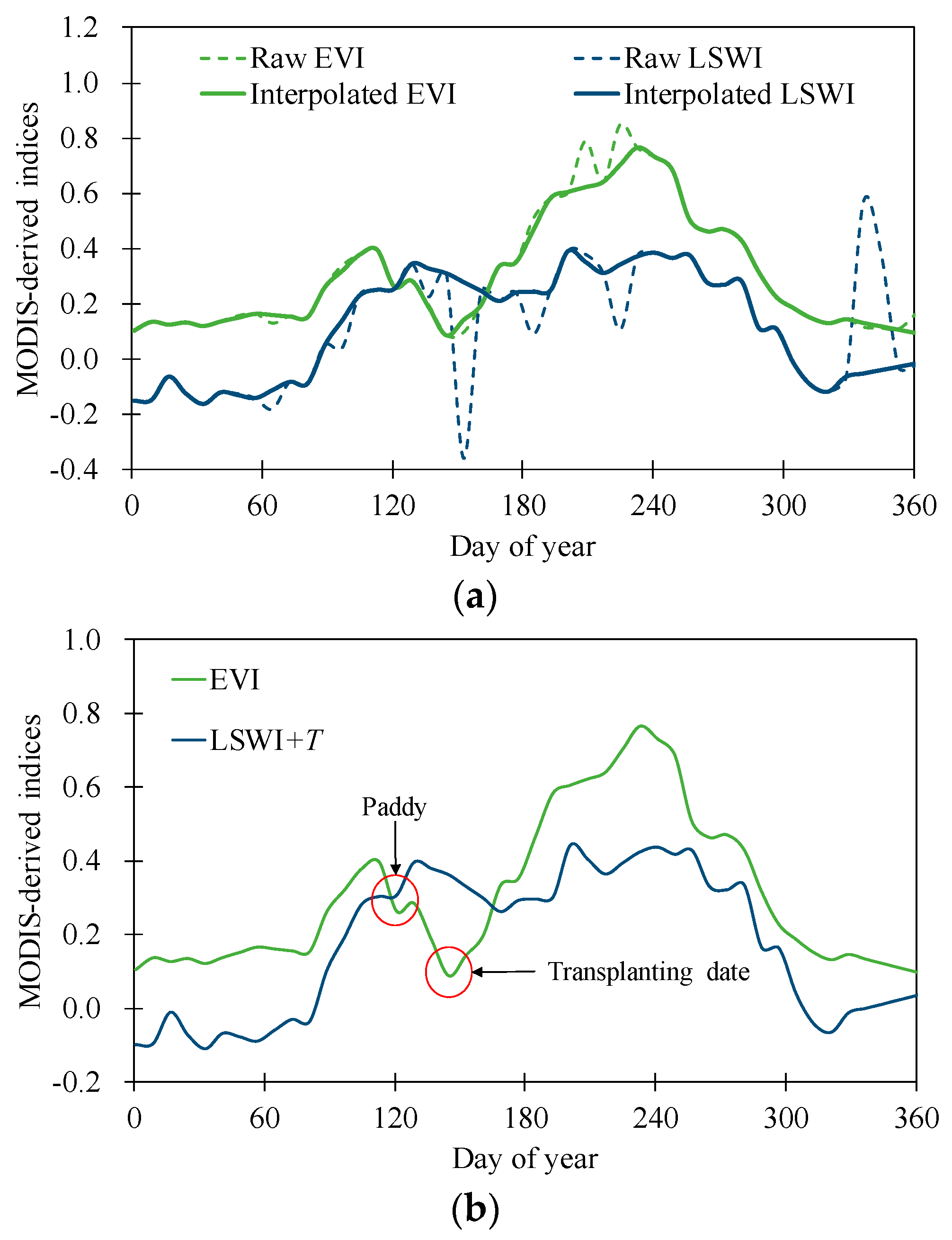
where , , , and are MODIS band 1 (red, 620–670 nm), band 2 (near infrared, NIR, 841–879 nm), band 3 (blue, 459–479 nm), and band 6 (short-wave infrared, SWIR, 1628–1652 nm) reflectances, respectively. Although the MODIS 8-day composite data can reduce the effect of clouds to some extent, abundant contaminated data can be present because the study area is usually cloudy during the crop growing season. Simple linear interpolation was performed to average the indices before and after the target indices. The insertion was conducted by using the QA cloud information and the blue band reflectance defined as having a value higher than 0.2 in the cloud-contaminated pixels (Figure 2a) [8,46].
The MCD12Q1 yearly product contains five land cover types characterizing different global land cover classification schemes. The primary land cover type is composed of 17 land cover classes that describe 11 natural vegetation classes, 3 developed and mosaicked land classes, and 3 non-vegetated land classes using the International Geosphere Biosphere Program (IGBP) scheme. The other four land cover classification schemes included the University of Maryland (UMD), MODIS-derived LAI/fPAR, MODIS-derived net primary production (NPP), and plant functional type (PFT). These MODIS products can be downloaded free of charge through the Level-1 and Atmosphere Archive and Distribution System (LDDAS) of the Distributed Active Archive Center (DAAC).
2.2.3. KLAPS Temperatures
Temperatures used as input biophysical parameters of the GRAMI-rice model were acquired from the Korea Local Analysis and Prediction System (KLAPS) provided by the Korea Meteorological Administration (KMA). The KLAPS is a numerical forecasting system including a real-time operating scheme to analyze and forecast weather conditions around the Korean Peninsula. The temperature data were reproduced by reanalysis weather data with 1.5 km spatial resolution and 70 levels from the ground surface up to the altitude where the atmospheric pressure reaches a 50 mbar (~40 km) in the vertical direction. In this study, we used temperature data at the height of 2 m above the ground. The weather data used include ground observation data from 470 Automated Weather Systems (AWS) and layered atmospheric weather data from Aircraft Communications Addressing and Reporting System (ACARS) [47]. Detailed information for the KLAPS procedure is given in Albers et al. [48] and McGinley et al. [49].
2.2.4. COMS Reflectance and Solar Insolation
COMS, which is the first geostationary orbit satellite of South Korea, was developed by the Korea Aerospace Research Institute (KARI) and launched on 27 June 2010. It is located at 36,000 km above the ground surface and along the longitude of 128.2°E. The COMS has four distinctive payloads: the GOCI for monitoring the ocean environment and short-term biological phenomena, the meteorological imager (MI) for monitoring weather phenomena and sea surface temperature (SST), S- and L-transponders for meteorology data dissemination, and the Ka-band transponder for communications. In this study, the reflectance and solar insolation data used as input parameters for simulation of rice yields and production were obtained from the GOCI and MI of COMS, respectively (Table 2).
GOCI reflectance data are provided as eight multi-spectral bands from visible to NIR with a 500 m spatial resolution every hour from 09:00 to 16:00 (local time). In this study, the GOCI reflectance was corrected for atmospheric effects by using the second simulation of the satellite signal in the solar spectrum (6S) model. The atmospheric inputs used in the 6S model were aerosol optical depth (AOD), water vapor, and the total ozone from MODIS products such as MOD04, MOD05, and MOD07. In addition, the semi-empirical bidirectional reflectance distribution function (BRDF) was applied to the GOCI reflectance data to correct the surface anisotropy effects. Among the eight-times hourly reflectance data obtained during the day, the values least affected by the aerosol and cloud were synthesized and reproduced as daily data. Further details of 6S and BRDF processing methods used for GOCI reflectance data are described in Yeom et al. [50]. Four VIs were calculated from the corrected GOCI reflectance to use as inputs of the crop model: normalized difference vegetation index (NDVI, Rouse, 1974), renormalized difference vegetation index (RDVI), optimized soil-adjusted vegetation index (OSAVI), and modified triangular vegetation index (MTVI). The equations for the four VIs are shown below [51,52,53,54].
where , , and are GOCI band 4 (green, 433–453 nm), band 5 (red, 650–670 nm), and band 8 (NIR, 845–885 nm) reflectances, respectively.
The COMS MI data were used to estimate daily solar insolation with a spatial resolution of 1 km using the Kawamura [55] physical model modified by Yemo et al. [56]. The model uses an improved cloud factor by using the visible reflectance and the solar zenith angle rather than the brightness temperature. The model also estimates a more accurate solar insolation considering the surface slope and elevation by using the DEM data. In the previous study, the estimated solar insolation data were validated by using 37 ground station pyranometers and the results showed reliability for both clear and cloudy sky conditions [56]. Details of the physical model and validation results are described in Yeom et al. [56].
2.3. Detection of Paddy Fields and Transplanting Dates
For the detection of paddy fields, MODIS reflectance, and land cover products were used. MODIS land cover data have been constructed and used worldwide and their reliability has been verified through various studies [57,58]. In this study, croplands were extracted from the MODIS land cover classes to detect the paddy fields among them. Croplands from the IGBP scheme that are primary land cover of MODIS were evaluated to have 83.3% of the producer’s accuracy and 92.8% of the user’s accuracy [57]. To ensure that the MODIS croplands include as many paddy fields as possible, all croplands for the five land cover types for three years from 2011 to 2013 were composited into one image. As shown in Table 3, the MODIS-based croplands included ~93% of all paddy fields. This study focuses on detecting the transplanted paddy fields and removing the non-paddy fields from the MODIS-based croplands.
Paddy rice has a unique style of growth in irrigated fields, which significantly differs from other staple crops. On the basis of this feature, Xiao et al. [46] proposed a threshold method for detecting paddy fields and transplanting dates using the interrelationships of EVI (or NDVI), LSWI, and the threshold (T) of the LSWI, i.e., the condition of LSWI + T ≥ EVI (Figure 2). EVI generally shows higher values than LSWI in dryland crop fields. Moreover, the irrigated or transplanting period in paddy fields temporally shows a reversal of the relationship between these indices because the short-wave infrared (SWIR) used in LSWI (Equation (2)) is highly sensitive to surface water. The T value applied to LSWI considers the mixed pixel effects of other land cover. The advantage of this approach is that detecting both paddy fields and transplanting dates of rice can be obtained by using the simple relation.
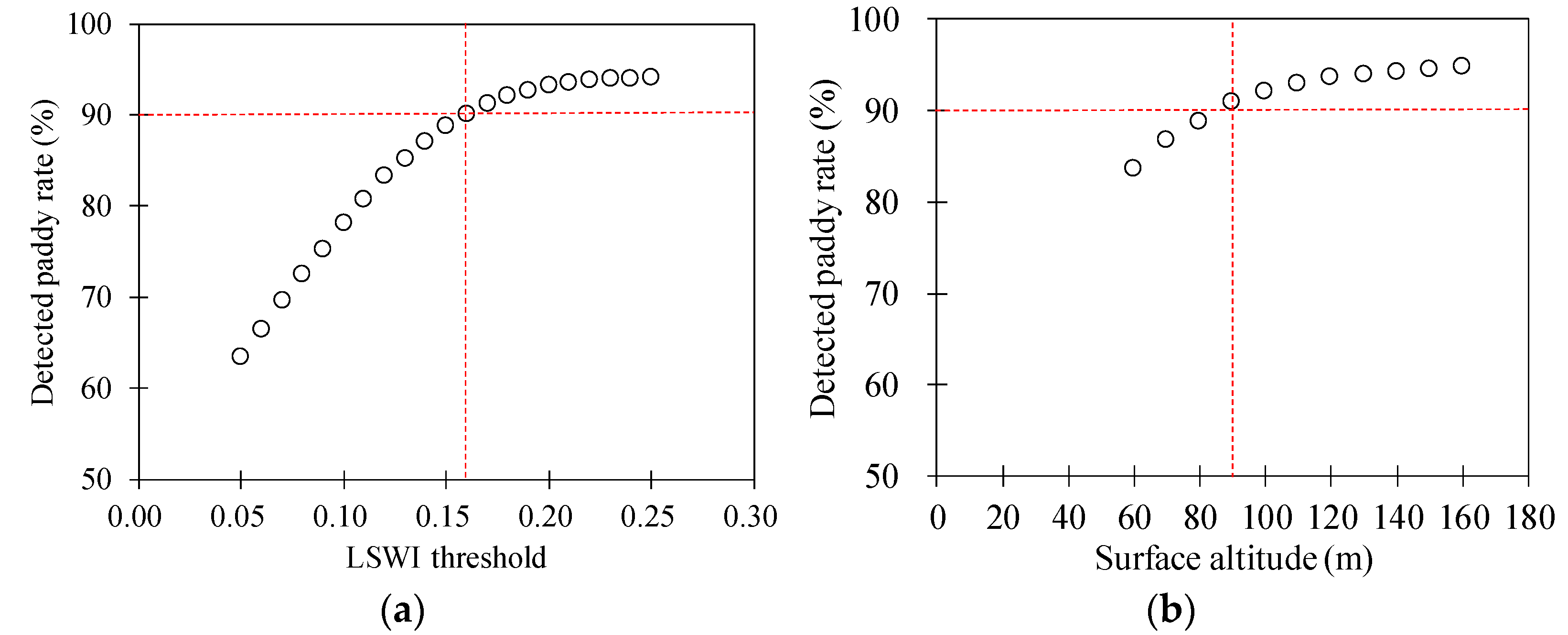
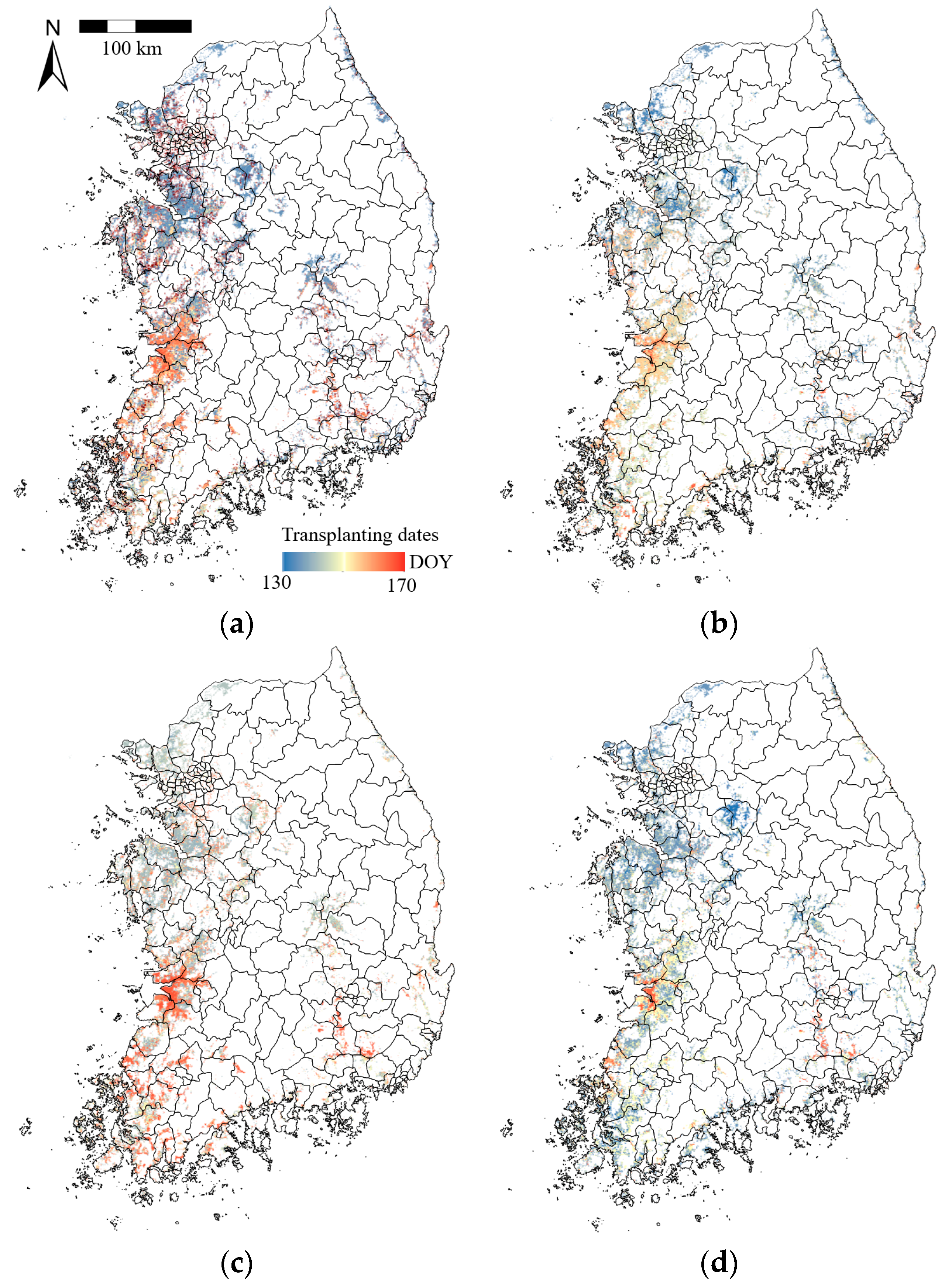
In this approach, the T value is an essential factor in determining the accuracy of the detected paddies, e.g., when the T value is too high, the detected paddy fields could be overestimated because the detection condition can be met even at lower EVI. Xiao et al. [46] suggested 0.05 as a global T value. However, other studies have reported that the T value should be changed, according to local land cover characteristics or cropping systems [7,59,60]. Sun et al. [59] proposed 0.17 as the T value for late transplanted rice and Peng et al. [7] used 0.21 for double-cropping fields. A method for applying different T values to each pixel according to land cover heterogeneity has also been reported [60]. In the current study, to determine the appropriate T value for the paddy fields in South Korea, the paddy fields were detected by using the threshold method while increasing the T value by 0.01 (Figure 3a). The value was determined to be the appropriate T value when the detected paddy field rates exceeded 90%, according to the KME-based paddy fields. MODIS-based reflectance values in 2013 were used to determine the T values and those in 2011, 2012, and 2014 were used to evaluate the detected paddy fields. The T value of this study area was determined as 0.16. Additionally, the transplanting dates of rice were estimated as those in which the EVI had the lowest values within the period satisfying the condition for detecting paddy fields (Figure 2b). Overall, the simulated transplanting dates in the southern sectors were later than those in the northern sectors (Figure 4). The transplanting times in the southern parts where temperatures are relatively high tended to be delayed because late-maturing varieties of rice are grown in those regions. These rice varieties are suitable in the southern sectors due to less sensitivity for the accumulation in growing degree days.
In the paddy fields detected using only the MODIS-based threshold method, misinterpretation of paddy patches can occur due to the effects of mixed land cover or poor pixels caused by clouds. The surface altitude and slope data from SRTM DEM were used to remove the erroneous paddy fields. In high-altitude regions in the study area, it is difficult to cultivate rice because of the low temperatures. Severe surface slopes also cause challenges in rice growth. Therefore, the threshold values of <90 m in surface altitude and <3° in slope were considered by using the same method as the one employed to select the T values (Figure 3b,c).
2.4. GRMAI-Rice Model for Simulation of Rice Yield and Production
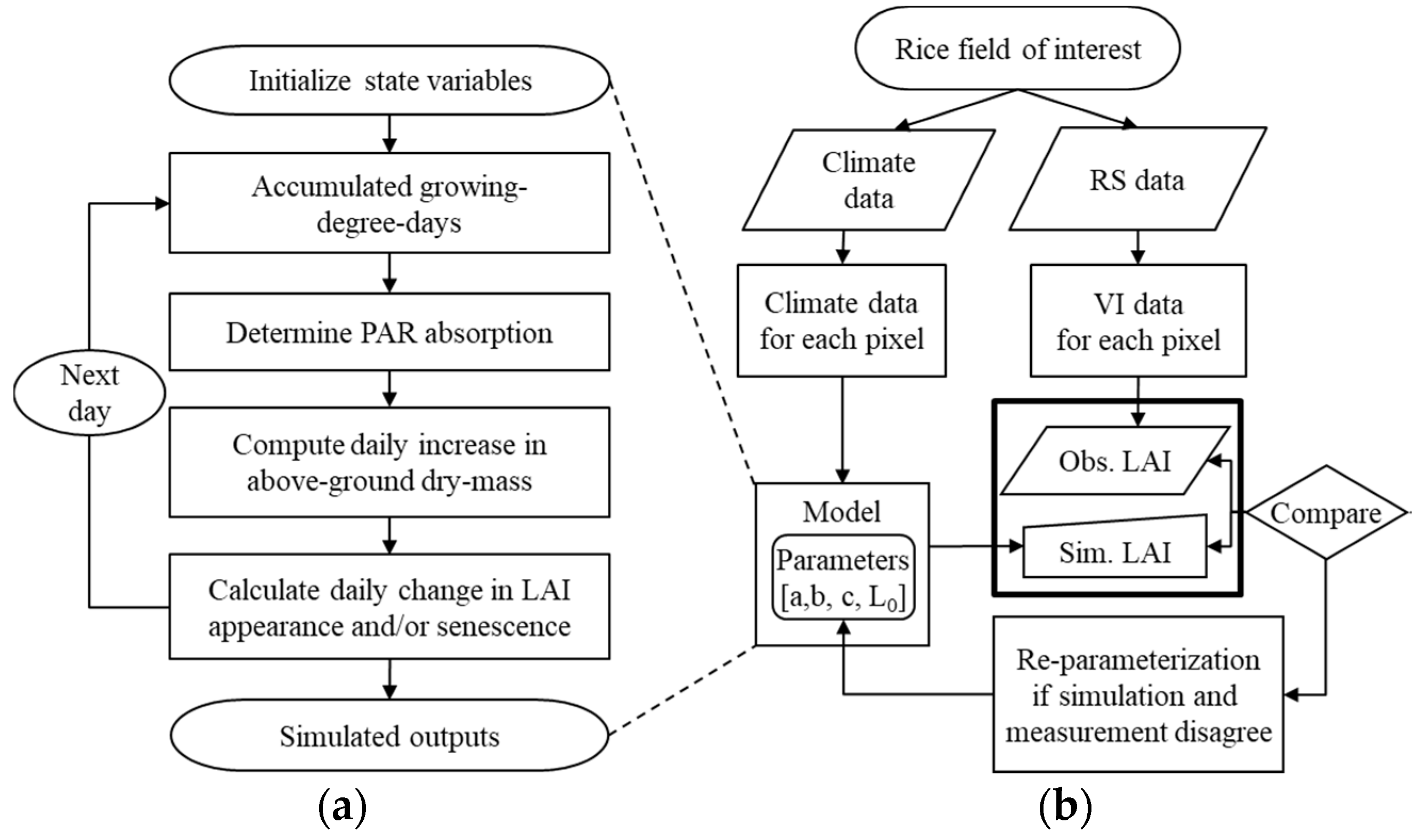
The grid-based GRAMI-rice model was used with GOCI satellite imagery to simulate rice yield and production for South Korea (Figure 5). The model was a modified and extended version to spatially simulate rice growth conditions and yield based on the GRAMI crop model [61]. The GRAMI model has three characteristics. First, the model can simulate crop yield by using only weather and remote sensing data as input variables and simple crop parameters unlike other process-based models that require many input variables and parameters. Second, it directly uses remote sensing data to simulate crop state variables such as LAI and yield. This feature makes the model highly dependent on remote sensing data. Therefore, reliable data acquisition is essential. Third, it employs a “within-season” calibration procedure that performs re-initialization to adjust the initial LAI of a crop and re-parameterization to modify the model parameters to determine an LAI seasonal curve by minimizing the difference between observed and simulated values [62,63]. This procedure can simulate daily LAI by using only several remotely spectral data for specific days during the crop growth season [41,62,63]. Further details are described in Maas [62,63] and Ko et al. [41].
The GRAMI-rice model was formulated to reproduce and monitor potential crop production information based on mathematical integration of remotely sensed information [41]. The crop model can receive remote sensing data as an input to execute the within-season calibration procedure. In this process, simulated crop canopy growth (LAI) is compared with the corresponding measured values to enable agreement with the measurement of a minimal error based on the parameterization of specified parameters. Four different coefficients (L0, a, b, and c) are employed in the model to describe the growth processes of rice. The parameter values were obtained through a parameterization process using the Bayesian method with a prior distribution chosen according to the estimates from previous reports. The relationships between five VIs and LAI were framed by using the log–log linear regression models as described later in this section.
The GRAMI-rice model includes four main processes for simulating rice growth and yield (Figure 5a). The first formulation is to calculate the growing degree days (GDD) of rice by using daily mean temperatures and a base temperature of rice. The second is to compute new dry mass produced by the rice canopy. The third is to determine the absorption of daily incident radiation energy by leaves using simulated LAI. Lastly, the fourth is to determine LAI partitioning from a new dry mass. The specific formulas are shown below. The accumulation of GDD was calculated by Equation (7) below.
where is the daily increase in GDD (°C), is the daily mean temperature (°C), and is the base temperature (°C) for rice, which was previously determined as 12 °C by Ko et al. [41]. The daily increase in the above ground dry mass (, g) was calculated by using the equation below.
where is the radiation use efficiency (RUE) of rice and is the daily total photosynthetically active radiation (PAR, MJ m−2). The rice was determined as 3.49 g MJ−1 [41]. was calculated by Equation (9) below.
where is the fraction of total solar irradiance (or fPAR), is the incident daily total solar irradiance (MJ m−2), and is the light extinction coefficient of rice. and were determined to be 0.45 by Monteith and Unsworth [64] and 0.6 by Charles-Edwards et al. [65], respectively. The daily LAI increase from new leaf growth () was calculated by the equation below.
where is the fraction of assigned to new leaves and is the specific leaf area (m2 g−1). was determined as 0.016 m2 g−1 [41]. was calculated by the equation below.
where and b are parameters that control the magnitude and shape of the function and D is the cumulative GDD (°C).
Rice yield (ton ha−1) was calculated by using the method below.
where ΔG is the daily increase in grain, P2 is the fraction of ΔM partitioned to grains, and ΔM is the daily increase in AGDW from Equation (8).
where P2 is the dimensionless grain-partitioning parameter, pa and pb are parameters that control the magnitude and shape of the function, and fGD is the grain partitioning factor based on the cumulative GDD. The county rice productions (kt) were calculated by multiplying simulated rice yields by the detected paddy areas (ha) in each county.
LAI is a three-dimensional concept while the reflectance of plants to solar radiation is a two-dimensional concept because the canopies of crops are the top surface of the plants. In the within-season calibration using the Bayesian method of parameter estimation, it was assumed that a log–log regression model with a slope of approximately 2/3 could describe the relationship between the reflectance and LAI. On the basis of this concept, the correlations between LAI and four VIs such as MTVI, NDVI, RDVI, and OSAVI were formulated by using log–log linear regression models. For each VI, labeled 1, 2, 3, 4, and 5, respectively, an empirical model was formulated, which is shown below.
where , and ( represent intercept, slope, and error of the linear regression model, respectively.
The evolution of the LAI for each pixel was explained by the GRAMI-rice model using four parameters (L0, a, b, and c). These parameters were assumed to be generated from the prior distribution , where the following transformations were used to guarantee that all four parameters (L0, a, b, and c) ranged between 0 and 1.
Both the regression coefficients and the hyper-parameters were obtained from the data collected in previous studies [40,41]. These include both the VIs and the measured LAI values. The parameter was specified by using the before-calibration values (L0 = 0.2, a = 3.25 × 10⁻¹, b = 1.25 × 10⁻³, and c = 1.25 × 10⁻³). Parameter D is a diagonal matrix with all diagonal elements equivalent to 0.5.
The following numerical procedure was adopted to obtain for each pixel.
- Step 1:
- For each pixel, set to serve as the initial estimation of .
- Step 2:
- Define and consider the objective function.
- Step 3:
- Generate the simulated curve for each pixel from the estimated ψ in Step 2.
- Step 4:
- Update μ, D as the sample means and sample variances of the estimates in Step 2.
In this procedure, the parameter ψ was estimated by minimizing the above function and the optimization was performed by using the POWELL optimization routine for one-point simulation cases and the Quasi-Newton minimizer for two-dimensional simulation cases [66,67].
The GRAMI model is designed to assimilate remote sensing data based on the mathematical procedures described above. The parameters of L0, a, and b control growth and development of crop canopies or LAI attributing to variation in crop yield and productivity (Figure 6). These parameters are reparametrized to make agreement between simulation and observation by using the minimization and optimization procedures.
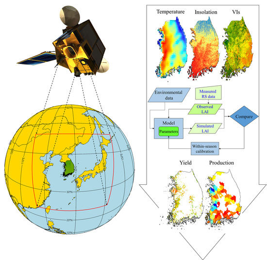
The Crop Information Delivery System (CIDS) was previously designed as an extended version of the GRAMI-rice model to project pixel-based geospatial crop growth and yield based on integration with remote sensing images (Figure 5b). CIDS employs pixel-based remote sensing data and climate data as system inputs and takes climate data either from a single weather station or multiple weather stations (pixels) depending on the situation. The GRAMI-rice model is then implemented to simulate crop growth in each pixel by using both types of input data. In CIDS, the GRAMI model simulates a crop in each pixel by using both remote sensing data and climate data as inputs [41].
2.5. Statistical Analysis
Statistical evaluations of the detected paddy areas and the simulated rice yield and production were performed by using two statistical indices called Nash–Sutcliffe efficiency (NSE) and the root-mean-square error (RMSE), which is shown below.
where , , , and n denote the ith simulated value, the ith measured value, the mean value, and the total number of values, respectively. The NSE ranges from −∞ to 1 in which the accuracy of the model performance is higher when the value is closer to 1. NSE values between 0 and 1 indicate that the simulated results are acceptable while values less than 0 mean that measured values are more dependable [68]. RMSE is a widely used measure of the difference between observed and simulated (or predicted) values. Values closer to 0 indicate closer agreement between the simulated and observed values. The two-paired t-test, which is a statistical analysis technique that compares the mean of two paired groups, was also performed. The observed rice dataset for the evaluation of the results was collected from KOSIS.
3. Results
3.1. Estimated Spatial Distribution of Paddy Fields and Transplanting Dates
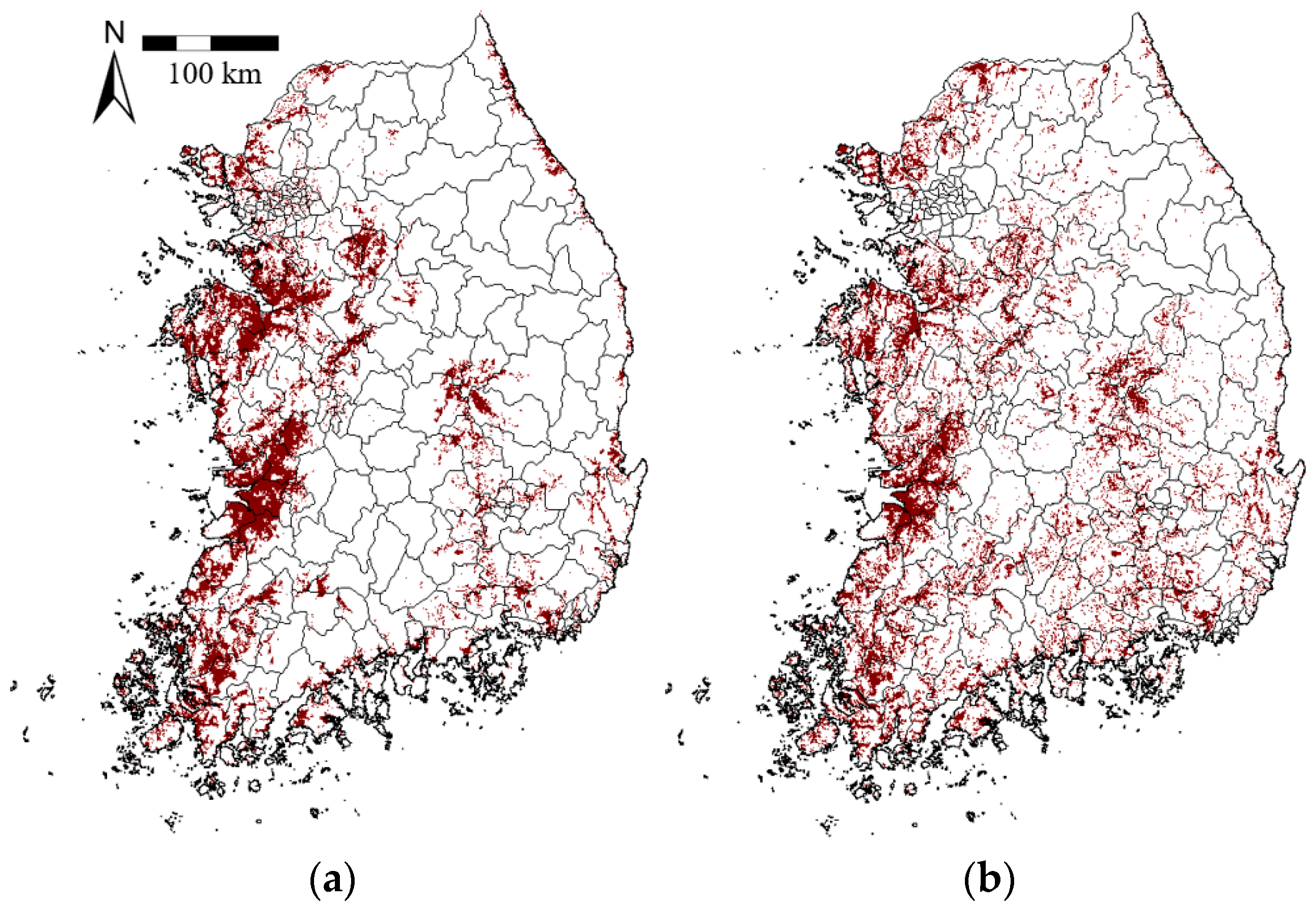
Paddy fields and transplanting dates of rice were estimated by using the approach proposed by Xiao et al. [46] prior to simulation of the rice yield and production using the GRAMI-rice model and the GOCI imagery. The threshold values of LSWI T, surface altitude, and surface slope were determined by using the KME-based paddy fields and MODIS-based spectral indices in 2013. In comparison with the KME-based land cover data, the overall accuracy for paddy and non-paddy fields was 90.2% in 2013. The overall accuracies when applying the determined thresholds in 2011, 2012, and 2014 were 89.5%, 90.1%, and 89.5%, respectively. In comparison with spatial distribution patterns between the KME-based and detected paddy fields, the broadly distributed paddy fields were in close agreement (Figure 7). However, scattered small paddy fields especially those situated near forests were poorly matched.
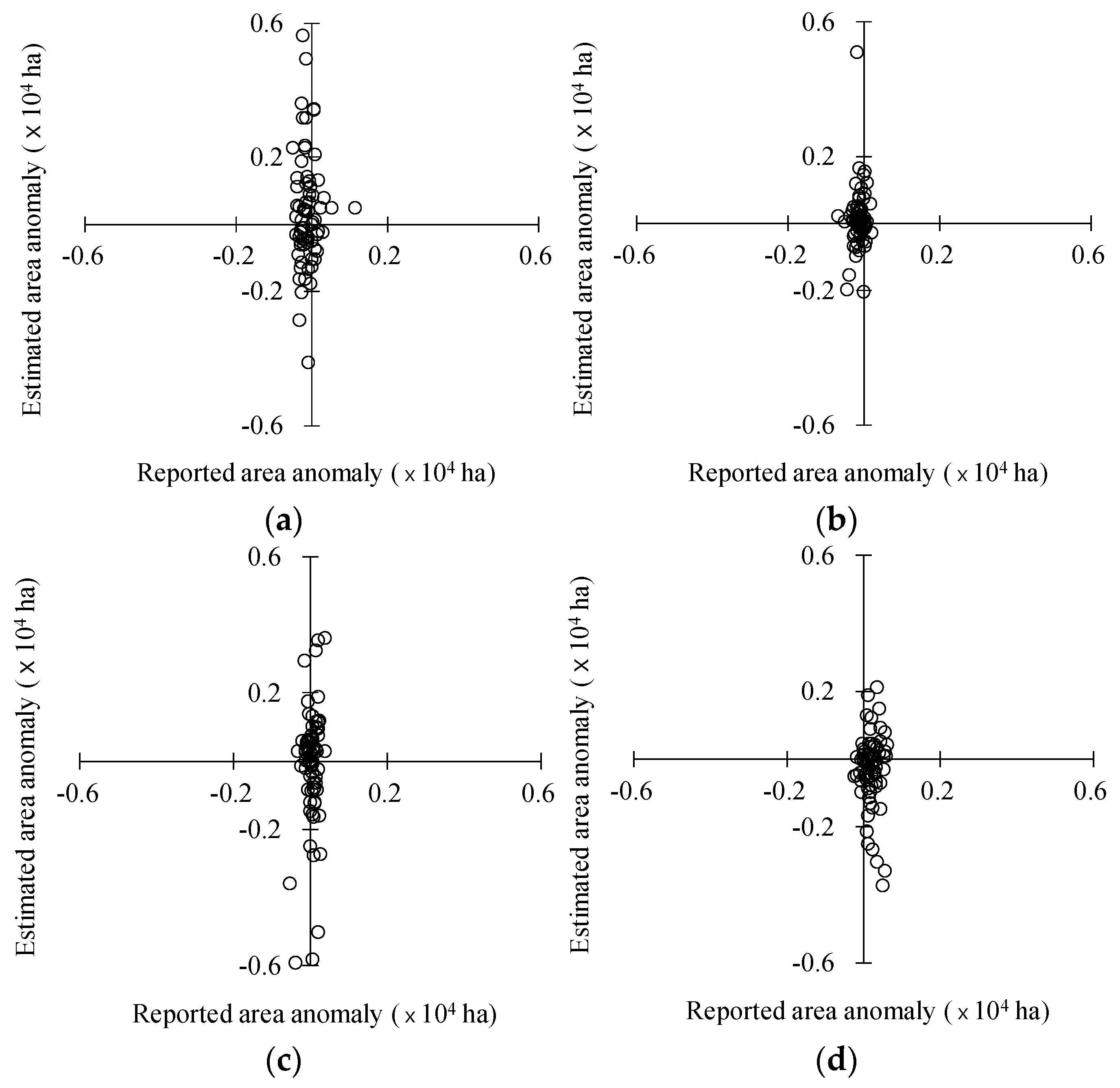
Additionally, the detected paddy areas were evaluated by using the observed paddy areas of more than 5000 ha in 73 counties obtained from KOSIS (Figure 8). The results showed that RMSE and NSE were 0.3982 × 10⁴ ha and 0.154 in 2011, 0.4266 × 10⁴ ha and 0.057 in 2012, 0.4755 × 10⁴ ha and −0.251 in 2013, and 0.4592 × 10⁴ ha and −0.198 in 2014, respectively (Table 4). Although the results in 2013 and 2014 disagreed somewhat, the paired t-tests revealed no significant differences between the observed and MODIS-derived paddy areas in which the p-values ranged from 0.331 to 0.980 in four years. Moreover, the observed and detected paddy areas showed high linearity in all four years in which the coefficient of determination (r2) ranged from 0.752 to 0.773 (Figure 8). In the comparison of anomalies in the paddy areas, there were larger anomalies in the estimation than those in the observation (Figure 9). While some yearly variations exist in the anomalies of the estimated paddy areas, the mean and median values of the anomalies did not deviate from the yearly mean and median values of the estimated paddy areas.
3.2. Evaluation of Simulated Rice Yields
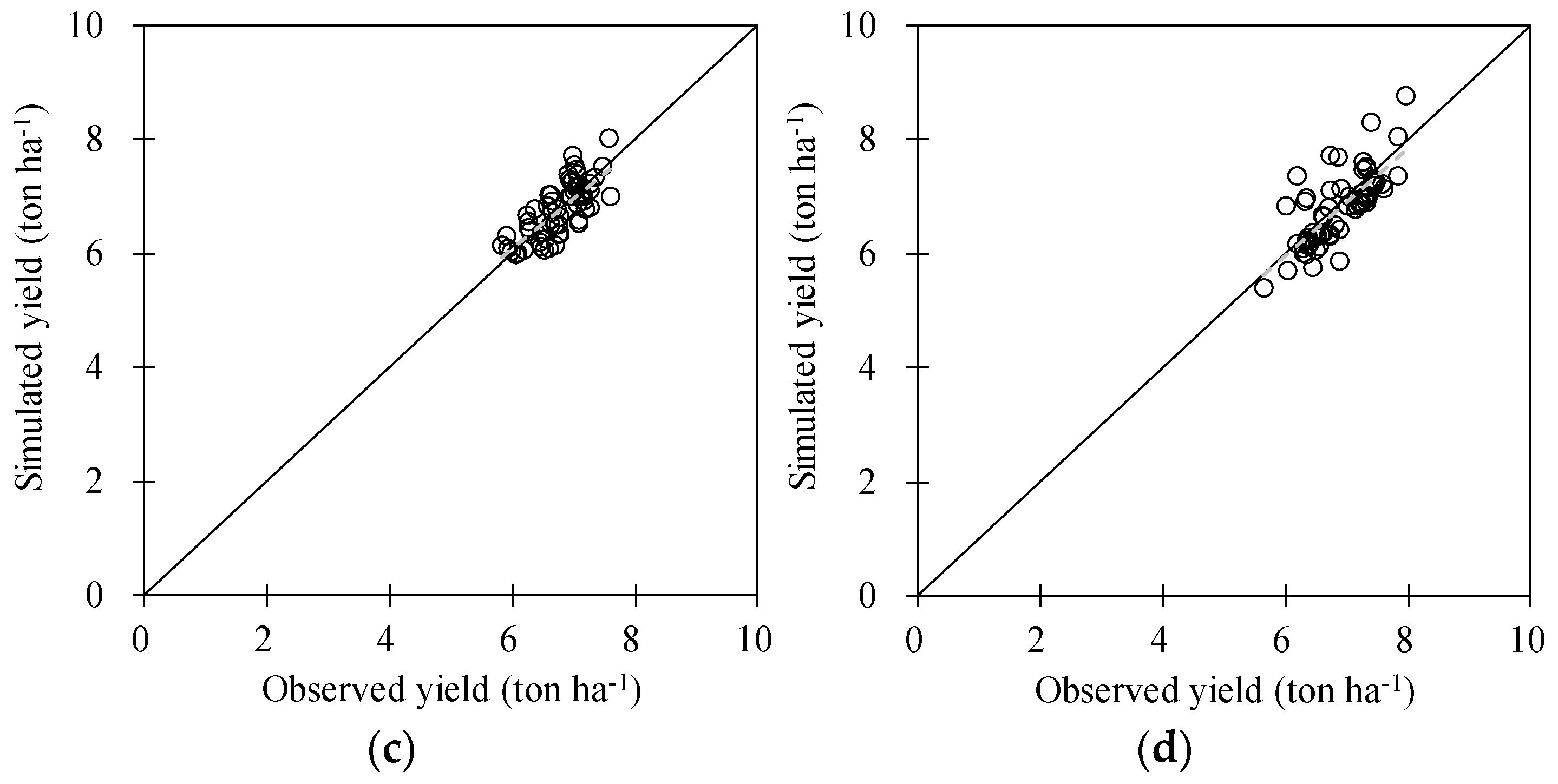
The GRAMI-rice model was calibrated using observed rice yields in 11 counties and was evaluated using those in 62 counties with more than 5000 ha of paddy areas in South Korea (Figure 1). The simulated rice yields were statistically in good agreement with the observed yields in the 11 counties (Figure 10). The RMSE and NSE values were 0.284 ton ha−1 and 0.627 in 2011, 0.324 ton ha−1 and 0.389 in 2012, 0.219 ton ha−1 and 0.733 in 2013, and 0.622 ton ha−1 and 0.692 in 2014, respectively (Table 5). According to the paired t-tests, the observed and simulated rice yields showed no significant differences with p-values of 0.732, 0.628, 0.545, and 0.692 in 2011, 2012, 2013, and 2014, respectively (Table 4).
The calibrated GRAMI-rice model was applied to the paddy fields detected by using the MODIS-based threshold method to project the spatial distribution of rice yield from 2011 to 2014 (Figure 11). Simulated yields were higher in the counties distributed in the central western region. In the northern and northeastern areas, simulated yields were relatively lower. A comparison of the observed and simulated rice yields for the 62 counties (Figure 12) revealed RMSE and NSE values of 0.374 ton ha−1 and 0.356 in 2011, 0.451 ton ha−1 and 0.486 in 2012, 0.326 ton ha−1 and 0.389 in 2013, and 0.441 ton ha−1 and 0.241 in 2014, respectively (Table 6). According to the paired t-tests, the simulated rice yields did not differ significantly from the observed yields with p-values of 0.404, 0.296, 0.815, and 0.392 in 2011, 2012, 2013, and 2014, respectively (Table 6).
3.3. Evaluation of Simulated Rice Production
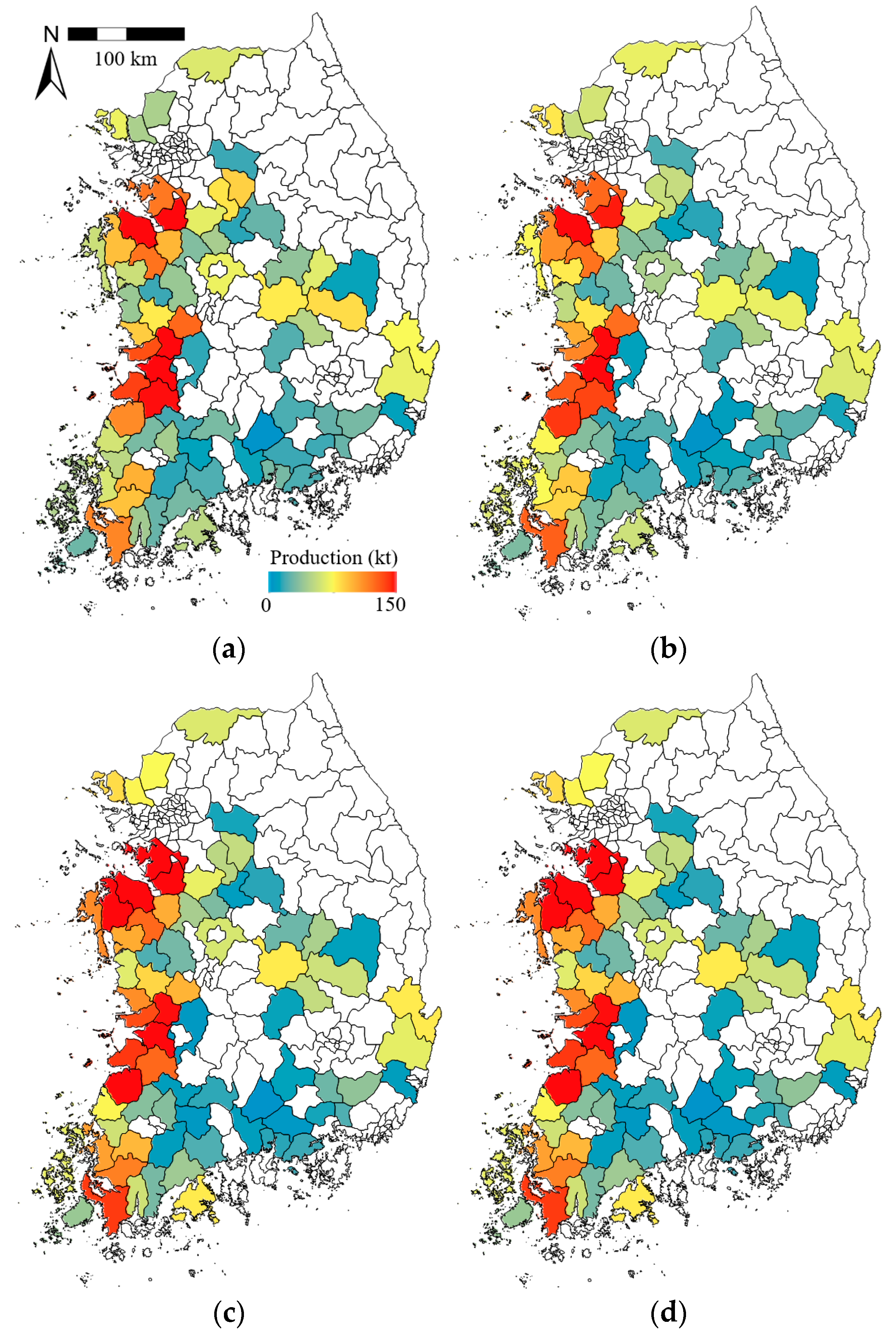
The simulated rice production in 73 counties with more than 5000 ha from 2011 to 2014 was calculated by using the simulated rice yield for each county and the estimated spatial distribution of the paddy fields (Figure 13). Overall, the simulated rice production in the western counties was higher than that in all other counties especially in the mid-western counties where the simulated rice yield was also higher. The paddy patches in the entire nation were distributed mainly in the plains and were stretched along the western and southern coastal regions. The spatial distribution of the simulated rice production effectively reflected the spatial characteristics of the plains in the entire study area.
A comparison of the observed and simulated rice production in 73 counties with more than 5000 ha in the study area (Figure 14) revealed RMSE and NSE values of 27.98 kt and 0.151 in 2011, 25.23 kt and 0.167 in 2012, 30.71 kt and −0.002 in 2013, and 33.00 kt and −0.123 in 2014, respectively (Table 7). In 2013 and 2014, the simulated rice production did not closely correspond to the measurements, which shows negative NSE values. However, according to the paired t-tests, no significant differences were noted between the observed and simulated rice productions with p-values of 0.893, 0.908, 0.579, and 0.337 in 2011, 2012, 2013, and 2104, respectively. Anomalies were larger in the estimation than the observation (Figure 15). The mean and median values of the anomalies did not deviate from the yearly mean in both the estimation and observation data while some yearly variations exist.
4. Discussion
The current study on the paddy area, the rice yield, and rice production focused on 73 counties in South Korea while KOSIS provided all of the data for a total of 97 counties. The other 24 counties were purposely excluded in this study because they contain many relatively small paddy fields. It is assumed that this issue could have resulted in undetected paddy fields, which might have affected the overall evaluation results. According to the analyses of RMSE and NSE, the paddy fields and production typically were not effectively reproduced in 2013 and 2014 (Table 3 and Table 6). Since the rice production was based on classified paddy pixels and simulated yield, the production accuracy was dependent on that of the estimated paddy fields and the simulated yield. The MODIS-derived paddy areas did not thoroughly agree with the observed paddy areas. Thus, the comparison results between the simulated and observed productions were similar to the evaluation results for the paddy areas (Figure 7 and Figure 12). Therefore, the simulated production errors can be explained by the disagreement of the MODIS image-based paddy fields with the actual paddy fields. The leading cause of the undetected paddy fields is attributable to the complicated land cover characteristics of the study area and the limitation of the satellite imagery with a coarse spatial resolution of 500 m. If a KME land cover map with a fine spatial resolution of 5 m is used, the rice yield and production could be simulated for most of the counties. Nevertheless, there are two reasons for detecting paddy fields using satellite imageries. The first is because the KME land cover data used in this study are updated at a quite slow cycle because they are obtained through direct supervised classification using various data points with high spatial resolution from aircraft or satellite platforms. Therefore, it is difficult to reflect seasonal changes in the spatial distribution of paddy patches. The second is attributed to a possible mismatch between the KME land cover map and the spectral information from satellite imagery. Paddy fields of the KME land cover data may not represent typical seasonal patterns of satellite-based VIs due to mixed pixel effects by various land cover types in the satellite images. Even if a reasonable number of paddy patches is shown within a 500 m pixel of a set of satellite images used for simulation, the simulated rice yield may not represent an actual value when the seasonal characteristics of rice cannot be expressed by using the same satellite data. If the seasonal patterns deviate from the distinctive patterns, errors can be severe because the GRAMI-rice model is highly dependent on remote sensing data [41,42]. Therefore, direct estimation of paddy fields in the area of interest using satellite imagery with the same spatial resolution would contain fewer errors for simulated yield using the crop model.
Despite the fact that using GOCI data can provide a more stable seasonal pattern and was used as the primary input variable for the GRAMI-rice model, the current study used MODIS data to detect the distribution of paddy fields. The reason is that paddy field has a unique characteristic of irrigation and MODIS LSWI is a very useful index to catch the irrigation. Besides detection of irrigation can be used to estimate the timing of the rice transplanting (beginning of the rice growth), which is an essential input of the crop model for the simulation of the yield. Another reason is that the irrigation period is not a monsoon season (from the middle of June to the end of August) so the MODIS data can provide relatively cloud-less VIs. There have been many studies using only a time series pattern of VIs without the LSWI to detect the paddy fields [5,69,70,71]. These features include maximum VIs values in the heading period, crop growth rates, or the growing period based on the seasonal patterns of the VIs. However, these approaches are not suitable for regions with many mixed pixels such as the current study area because the spectral characteristics of crops can be lost. However, the LSWI-based approach used in this study is highly sensitive to irrigation water, which makes it relatively accurate for paddy detection in mixed land cover regions [60,72]. An additional approach is available for using GOCI-based EVI (or NDVI) and MODIS-based LSWI. However, it requires further verification because the spectral response characteristics of the GOCI data are somewhat different from those of the MODIS data [14,50]. In addition, this approach may contain errors caused by a projection difference between both imagery types. Despite these reasons, using MODIS and GOCI imagery together might increase the accuracy of paddy detection in future research because GOCI images can provide stable seasonal VIs.
Scattered paddy patches with a small scale were not detected well in the MODIS-based paddy fields mainly because of the coarse spatial resolution of MODIS images. Although the KME land cover data were resampled into a spatial resolution of 500 m, they still reflected small-scale paddy fields because they are based on a spatial resolution of 5 m. It might be unreasonable to compare the two dissimilar data points with such variance in spatial resolution. In previous studies, evaluation was performed mainly by comparing the paddy area rather than spatial distribution [8,46,73,74]. However, because evaluation of spatial distribution accuracy is apparently a necessary factor, development of a statistical evaluation technique for comparing data with different spatial resolutions is needed. Another reason is that the scattered paddy fields are distributed near forests with a small scale, which can be removed together in the process of eliminating non-paddy fields by using the thresholds for surface altitude and slope. In this study, the thresholds were defined as paddy fields exceeding 90% of the total paddy fields because non-paddy fields increase inversely if the threshold criterion is higher. The most challenging aspect of the approach using thresholds is how to determine an appropriate threshold value that can vary depending on land cover composition or land surface characteristics of the study area [7,60]. This study used thresholds that can ignore small paddy fields in consideration of the coarse spatial resolution of MODIS images. However, when using satellite images of a higher spatial resolution or those applied to other regions, the thresholds can be different. In addition, the KME-based paddy fields include fallow land while MODIS-based paddy fields can detect only arable land, which also results in an error.
The simulated rice yields were in statistically acceptable agreement with the observed yields in most counties of South Korea from 2011 to 2014. Some error was caused apparently by subpixel heterogeneity. However, the simulated rice yields were similar to the corresponding observed values, which demonstrates relatively high reliability. The results of the current study are comparable with those of earlier studies using the GRAMI model [39,40,41,42]. Although the previous evaluated the performance of the GRAMI model in farm fields or small-region to mid-region scales, the current study focuses on the application at the scale of an entire nation. Therefore, the simulation outcomes using the GRAMI model and satellite imagery would be potentially applicable for crop management as a decision support system in various fields and regions and can provide crop productivity information for an entire nation.
According to the statistical analyses for the simulated rice yield by year, RMSE was the highest in 2012 at 0.451 ton ha−1 and NSE was the lowest in 2014 at 0.241. The simulation errors in 2012 were higher in southern counties while those in 2014 were higher in the northern counties (Figure 14). Drought was severe in 2012 and 2014 (data not shown), according to a report by the National Drought Information Analysis Center (NDIAC) of South Korea. In 2012, the drought occurred throughout the country from May to June. As a result, the observed rice yield in the southern region was affected severely, which resulted in a yield lower than that in other years. In 2014, the drought had a severe influence in the northern sectors. It was assumed that the model could not effectively simulate conditions when the rice yield was lower than average or when the values deviated from the yields used in calibration.
The input parameters used in the model can result in potential error factors. Among them, the parameters for the relationships between specific VIs and LAI are crucial factors that can have an essential impact on the simulation results. Doraiswamy et al. [1] reported that the relationship between canopy NDVI and LAI used in the calibration procedure might not be consistent in all applied research areas due to differences in soil characteristics, plant populations, and other factors. Ko et al. [41] and Moulin et al. [36] reported that the error can be severe if the collected relationships between LAI and VIs exceed the range. To minimize this issue, log–log linear regression models were introduced to formulate the correlations between LAI and four VIs such as MTVI, NDVI, RDVI, and OSAVI collectively. It was presumed that a log–log regression model with a slope of approximately 2/3 could describe the relationship between reflectance (VI) and LAI. The GRAMI-rice model is theoretically incorporated with a Bayesian method for parameter estimation to facilitate an agreement between simulations and observations based on the Quasi–Newton optimization procedure for two-dimensional simulation cases [67]. The current parameter estimation method was considered to be favorable for integrating various remote sensing data into crop models that have a strong dependence on input LAI from remotely sensed information. The solid assimilation of the current GRAMI model with remote sensing data can offer distinct benefits in several ways. First, the current approach allows a simple input condition, which employs only the existing observations that characterize the environmental conditions. Second, the optimization method enables the GRAMI model to improve the simulation performance. Third, the GRAMI model can be combined with remotely sensed information from various platforms such as an unmanned aerial system (UAS) and operational optical satellites including sensors of various spatial resolution [14,40,42]. Lastly, the model is applicable for any region of interest on the Earth’s surface depending on the availability of satellite imagery. However, limitations include inadequate representation of remotely sensed information as well as restricted observations available during the crop growing season. These limits can eventually cause some level of disagreement between simulations and observations. Although some limitations in the GRAMI model exist including a steady dependence on the remote sensing data needed to accomplish the modeling mentioned above, the requisite of input parameters and variables has significant implications especially for inaccessible and data-sparse regions. In such regions, this type of crop model is particularly significant because it is almost impossible to monitor or project the crop productivity without using operational satellite imagery.
5. Conclusions
In this study, regional rice productions were estimated from detected paddy fields and simulation of rice yield for 73 counties of South Korea from 2011 to 2014. The paddy fields were classified using MODIS imagery and the rice yield was simulated by using the GRAMI-rice model combined with GOCI imagery. Despite the subpixel heterogeneity of satellite images because of coarse spatial resolution, the overall accuracy analysis results were statistically acceptable and reasonable considering the national scale of the study. Therefore, this study may help manage staple food production in the country by providing an accurate understanding of the current circumstances for the regional crop productivity based on the crop model integrated with GOCI images. The GOCI satellite can continuously and reliably obtain surface reflectance in the Northeast Asia region near the Korean Peninsula. It is believed that the combination of the crop model and GOCI imagery could help implement diagnostic information monitoring and can offer a delivery system that can project crop growth conditions and monitor regional crop yield and production in Northeast Asia.
Author Contributions
S.J. designed the research direction, conducted the research, and wrote the manuscript. J.K. contributed the research design, developed the crop model, and reviewed the manuscript. J.Y. contributed the research design, processed, and analyzed the whole satellite data. All authors were equally involved in the editing of the manuscript.
Funding
This research was supported by the Basic Science Research Program through the National Research Foundation of Korea (NRF) and funded by the Ministry of Education, Science, and Technology (NRF-2015R1D1A1A01057586).
Acknowledgments
The authors thank the Korea Institute of Ocean Science and Technology (KIOST) for providing the GOCI data.
Conflicts of Interest
The authors declare no conflict of interest.
References
- Doraiswamy, P.C.; Sinclair, T.R.; Hollinger, S.; Akhmedov, B.; Stern, A.; Prueger, J. Application of MODIS derived parameters for regional crop yield assessment. Remote Sens. Environ. 2005, 97, 192–202. [Google Scholar] [CrossRef]
- Lobell, D.B.; Thau, D.; Seifert, C.; Engle, E.; Little, B. A scalable satellite-based crop yield mapper. Remote Sens. Environ. 2015, 164, 324–333. [Google Scholar] [CrossRef]
- Mo, X.G.; Liu, S.X.; Lin, Z.H.; Xu, Y.Q.; Xiang, Y.; McVicar, T.R. Prediction of crop yield, water consumption and water use efficiency with a SVAT-crop growth model using remotely sensed data on the north china plain. Ecol. Model. 2005, 183, 301–322. [Google Scholar] [CrossRef]
- Peng, D.L.; Huang, J.F.; Li, C.J.; Liu, L.Y.; Huang, W.J.; Wang, F.M.; Yang, X.H. Modelling paddy rice yield using MODIS data. Agric. For. Meteorol. 2014, 184, 107–116. [Google Scholar] [CrossRef]
- Johnson, D.M. A comprehensive assessment of the correlations between field crop yields and commonly used MODIS products. Int. J. Appl. Earth Obs. Geoinf. 2016, 52, 65–81. [Google Scholar] [CrossRef] [Green Version]
- Huang, N.E.; Shen, Z.; Long, S.R.; Wu, M.C.; Shih, H.H.; Zheng, Q.; Yen, N.-C.; Tung, C.C.; Liu, H.H. The empirical mode decomposition and the hilbert spectrum for nonlinear and non-stationary time series analysis. In Proceedings of the Royal Society of London A: Mathematical, Physical and Engineering Sciences 454, The Royal Society, London, UK, 8 March 1998; pp. 903–995. [Google Scholar]
- Peng, D.L.; Huete, A.R.; Huang, J.F.; Wang, F.M.; Sun, H.S. Detection and estimation of mixed paddy rice cropping patterns with MODIS data. Int. J. Appl. Earth. Obs. Geoinf. 2011, 13, 13–23. [Google Scholar] [CrossRef]
- Sakamoto, T.; Van Nguyen, N.; Kotera, A.; Ohno, H.; Ishitsuka, N.; Yokozawa, M. Detecting temporal changes in the extent of annual flooding within the Cambodia and the Vietnamese Mekong Delta from MODIS time-series imagery. Remote Sens. Environ. 2007, 109, 295–313. [Google Scholar] [CrossRef]
- Justice, C.O.; Townshend, J.R.G.; Holben, B.N.; Tucker, C.J. Analysis of the phenology of global vegetation using meteorological satellite data. Int. J. Remote Sens. 2007, 6, 1271–1318. [Google Scholar] [CrossRef]
- Gao, F.; Morisette, J.T.; Wolfe, R.E.; Ederer, G.; Pedelty, J.; Masuoka, E.; Myneni, R.; Tan, B.; Nightingale, J. An algorithm to produce temporally and spatially continuous MOIDS_LAI time series. IEEE Geosci. Remote Sens. Lett. 2008, 5, 60–64. [Google Scholar] [CrossRef]
- Jiang, B.; Liang, S.L.; Wang, J.D.; Xiao, Z.Q. Modeling MODIS LAI time series using three statistical methods. Remote Sens. Environ. 2010, 114, 1432–1444. [Google Scholar] [CrossRef]
- Kandasamy, S.; Baret, F.; Verger, A.; Neveux, P.; Weiss, M. A comparison of methods for smoothing and gap filling time series of remote sensing observations–Application to MODIS LAI products. Biogeosciences 2013, 10, 4055–4071. [Google Scholar] [CrossRef]
- Funk, C.; Budde, M.E. Phenologically-tuned MODIS-NDVI-based production anomaly estimates for Zimbabwe. Remote Sens. Environ. 2009, 113, 115–125. [Google Scholar] [CrossRef]
- Yeom, J.M.; Kim, H.O. Comparison of NDVI from GOCI and MODIS data towards improved assessment of crop temporal dynamics in the case of paddy rice. Remote Sens. 2015, 7, 11326–11343. [Google Scholar] [CrossRef]
- Fensholt, R.; Anyamba, A.; Stisen, S.; Sandholt, I.; Pak, E.; Small, J. Comparisons of compositing period length for vegetation index data from polar-orbiting and geostationary satellites for the cloud-prone region of West Africa. Photogramm. Eng. Remote Sens. 2007, 73, 297–309. [Google Scholar] [CrossRef]
- Nigam, R.; Vyas, S.S.; Bhattacharya, B.K.; Oza, M.P.; Manjunath, K.R. Retrieval of regional LAI over agricultural land from an Indian geostationary satellite and its application for crop yield estimation. J. Spat. Sci. 2016, 1–23. [Google Scholar] [CrossRef]
- Nigam, R.; Bhattacharya, B.K.; Gunjal, K.R.; Padmanabhan, N.; Patel, N.K. Formulation of time series vegetation index from Indian geostationary satellite and comparison with global product. J. Indian Soc. Remote Sens. 2012, 40, 1–9. [Google Scholar] [CrossRef]
- Doraiswamy, P.C.; Cook, P.W. Spring wheat yield assessment using NOAA AVHRR data. Can. J. Remote Sens. 1995, 21, 43–51. [Google Scholar] [CrossRef]
- Groten, S.M.E. NDVI—Crop monitoring and early yield assessment of Burkina Faso. Int. J. Remote Sens. 1993, 14, 1495–1515. [Google Scholar] [CrossRef]
- Weiss, L.M.; Marcy, G.W. The mass-radius relation for 65 exoplanets smaller than 4 Earth radii. Astrophys. J. Lett. 2014, 783, L6. [Google Scholar] [CrossRef]
- Lobell, D.B.; Asner, G.P.; Ortiz-Monasterio, J.I.; Benning, T.L. Remote sensing of regional crop production in the Yaqui Valley, Mexico: Estimates and uncertainties. Agric. Ecosyst. Environ. 2003, 94, 205–220. [Google Scholar] [CrossRef]
- Monteith, J.L.; Moss, C. Climate and the efficiency of crop production in Britain. Philos. Trans. R. Soc. Lond. B Biol. Sci. 1977, 281, 277–294. [Google Scholar] [CrossRef]
- Doraiswamy, P.C.; Hatfield, J.L.; Jackson, T.J.; Akhmedov, B.; Prueger, J.; Stern, A. Crop condition and yield simulations using Landsat and MODIS. Remote Sens. Environ. 2004, 92, 548–559. [Google Scholar] [CrossRef]
- Chang, I.S.; Wu, J. Integration of climate change considerations into environmental impact assessment—Implementation, problems and recommendations for China. Front. Environ. Sci. Eng. 2013, 7, 598–607. [Google Scholar] [CrossRef]
- Gaudin, A.C.; Tolhurst, T.N.; Ker, A.P.; Janovicek, K.; Tortora, C.; Martin, R.C.; Deen, W. Increasing crop diversity mitigates weather variations and improves yield stability. PLoS ONE 2015, 10, e0113261. [Google Scholar] [CrossRef] [PubMed]
- Jones, J.W.; Hoogenboom, G.; Porter, C.H.; Boote, K.J.; Batchelor, W.D.; Hunt, L.A.; Wilkens, P.W.; Singh, U.; Gijsman, A.J.; Ritchie, J.T. The DSSAT cropping system model. Eur. J. Agron. 2003, 18, 235–265. [Google Scholar] [CrossRef]
- Stockle, C.O.; Donatelli, M.; Nelson, R. Cropsyst, a cropping systems simulation model. Eur. J. Agron. 2003, 18, 289–307. [Google Scholar] [CrossRef]
- Moriondo, M.; Maselli, F.; Bindi, M. A simple model of regional wheat yield based on NDVI data. Eur. J. Agron. 2007, 26, 266–274. [Google Scholar] [CrossRef]
- Ritchie, J.; Godwin, D.; Otter-Nacke, S. Ceres-Wheat. A Simulation Model of Wheat Growth and Development; Texas A&M: College Station, TX, USA, 1985. [Google Scholar]
- Barnes, E.M.; Pinter, P.J.; Kimball, B.A.; Wall, G.W.; LaMorte, R.L.; Hunsaker, D.J.; Adamsen, F.; Leavitt, S.; Thompson, T.; Mathius, J. Modification of Ceres-wheat to accept leaf area index as an input variable. In Proceedings of the 1997 ASAE Annual International Meeting, Minneapolis, MN, USA, 10–14 August 1997. [Google Scholar]
- Huang, J.X.; Sedano, F.; Huang, Y.B.; Ma, H.Y.; Li, X.L.; Liang, S.L.; Tian, L.Y.; Zhang, X.D.; Fan, J.L.; Wu, W.B. Assimilating a synthetic Kalman filter leaf area index series into the WOFOST model to improve regional winter wheat yield estimation. Agric. For. Meteorol. 2016, 216, 188–202. [Google Scholar] [CrossRef]
- Launay, M.; Guerif, M. Assimilating remote sensing data into a crop model to improve predictive performance for spatial applications. Agric. Ecosyst. Environ. 2005, 111, 321–339. [Google Scholar] [CrossRef]
- Zhao, Y.X.; Chen, S.N.; Shen, S.H. Assimilating remote sensing information with crop model using ensemble Kalman filter for improving LAI monitoring and yield estimation. Ecol. Model. 2013, 270, 30–42. [Google Scholar] [CrossRef]
- Spitters, C.; Van Keulen, H.; Van Kraalingen, D. A simple and universal crop growth simulator: Sucros87. In Simulation and Systems Management in Crop Protection; Pudoc: Wageningen, The Netherlands, 1989; pp. 147–181. [Google Scholar]
- Delécolle, R.; Maas, S.; Guérif, M.; Baret, F. Remote sensing and crop production models: Present trends. ISPRS J. Photogramm. Remote Sens. 1992, 47, 145–161. [Google Scholar] [CrossRef]
- Moulin, S.; Bondeau, A.; Delecolle, R. Combining agricultural crop models and satellite observations: From field to regional scales. Int. J. Remote Sens. 1998, 19, 1021–1036. [Google Scholar] [CrossRef]
- Huang, Y.; Ryu, Y.; Jiang, C.; Kim, H.; Kim, S.; Kang, M.; Shim, K. Bess-rice: A remote sensing derived and biophysical process-based rice productivity simulation model. Agric. For. Meteorol. 2018, 256, 253–269. [Google Scholar] [CrossRef]
- Maas, S.J. GRAMI: A Crop Growth Model that Can Use Remotely Sensed Information; ARS-91, US Department of Agriculture, Agricultural Research Service: Washington, DC, USA, 1992.
- Padilla, F.L.M.; Maas, S.J.; Gonzalez-Dugo, M.P.; Mansilla, F.; Rajan, N.; Gavilan, P.; Dominguez, J. Monitoring regional wheat yield in Southern Spain using the GRAMI model and satellite imagery. Field Crop Res. 2012, 130, 145–154. [Google Scholar] [CrossRef]
- Kim, M.; Ko, J.; Jeong, S.; Yeom, J.M.; Kim, H.O. Monitoring canopy growth and grain yield of paddy rice in South Korea by using the GRAMI model and high spatial resolution imagery. Gisci. Remote Sens. 2017, 54, 534–551. [Google Scholar] [CrossRef]
- Ko, J.; Jeong, S.; Yeom, J.; Kim, H.; Ban, J.O.; Kim, H.Y. Simulation and mapping of rice growth and yield based on remote sensing. J. Appl. Remote Sens. 2015, 9, 096067. [Google Scholar] [CrossRef]
- Jeong, S.; Ko, J.; Choi, J.; Xue, W.; Yeom, J.M. Application of an unmanned aerial system for monitoring paddy productivity using the GRAMI-rice model. Int. J. Remote Sens. 2018, 39, 2441–2462. [Google Scholar] [CrossRef]
- Rabus, B.; Eineder, M.; Roth, A.; Bamler, R. The shuttle radar topography mission-a new class of digital elevation models acquired by spaceborne radar. ISPRS J. Photogramm. Remote Sens. 2003, 57, 241–262. [Google Scholar] [CrossRef]
- Gao, B.-C. NDWI—A normalized difference water index for remote sensing of vegetation liquid water from space. Remote Sens. Environ. 1996, 58, 257–266. [Google Scholar] [CrossRef]
- Huete, A.; Didan, K.; Miura, T.; Rodriguez, E.P.; Gao, X.; Ferreira, L.G. Overview of the radiometric and biophysical performance of the MODIS vegetation indices. Remote Sens. Environ. 2002, 83, 195–213. [Google Scholar] [CrossRef]
- Xiao, X.M.; Boles, S.; Liu, J.Y.; Zhuang, D.F.; Frolking, S.; Li, C.S.; Salas, W.; Moore, B. Mapping paddy rice agriculture in Southern China using multi-temporal MODIS images. Remote Sens. Environ. 2005, 95, 480–492. [Google Scholar] [CrossRef]
- Kim, Y.; Park, O.; Hwang, S. Realtime operation of the Korea local analysis and prediction system at METRI. Asia Pac. J. Atmos. Sci. 2002, 38, 1–10. [Google Scholar]
- Albers, S.C.; McGinley, J.A.; Birkenheuer, D.L.; Smart, J.R. The local analysis and prediction system (LAPS): Analyses of clouds, precipitation, and temperature. Weather Forecast. 1996, 11, 273–287. [Google Scholar] [CrossRef]
- McGinley, J.A.; Albers, S.C.; Stamus, P.A. Validation of a composite convective index as defined by a real-time local analysis system. Weather Forecast. 1991, 6, 337–356. [Google Scholar] [CrossRef]
- Yeom, J.M.; Kim, H.O. Feasibility of using geostationary ocean colour imager (GOCI) data for land applications after atmospheric correction and bidirectional reflectance distribution function modelling. Int. J. Remote Sens. 2013, 34, 7329–7339. [Google Scholar] [CrossRef]
- Rouse, J.W., Jr.; Haas, R.; Schell, J.; Deering, D. Monitoring Vegetation Systems in the Great Plains with ERTS; Texas A&M Univ., College Station: Texas, USA, 1974. [Google Scholar]
- Roujean, J.L.; Breon, F.M. Estimating PAR absorbed by vegetation from bidirectional reflectance measurements. Remote Sens. Environ. 1995, 51, 375–384. [Google Scholar] [CrossRef]
- Rondeaux, G.; Steven, M.; Baret, F. Optimization of soil-adjusted vegetation indices. Remote Sens. Environ. 1996, 55, 95–107. [Google Scholar] [CrossRef]
- Haboudane, D.; Miller, J.R.; Pattey, E.; Zarco-Tejada, P.J.; Strachan, I.B. Hyperspectral vegetation indices and novel algorithms for predicting green LAI of crop canopies: Modeling and validation in the context of precision agriculture. Remote Sens. Environ. 2004, 90, 337–352. [Google Scholar] [CrossRef]
- Kawamura, H.; Tanahashi, S.; Takahashi, T. Estimation of insolation over the Pacific Ocean off the Sanriku coast. J. Oceanogr. 1998, 54, 457–464. [Google Scholar] [CrossRef]
- Yeom, J.M.; Seo, Y.K.; Kim, D.S.; Han, K.S. Solar radiation received by slopes using COMS imagery, a physically based radiation model, and GLOBE. J. Sens. 2016, 2016, 4834579. [Google Scholar] [CrossRef]
- Friedl, M.A.; Sulla-Menashe, D.; Tan, B.; Schneider, A.; Ramankutty, N.; Sibley, A.; Huang, X.M. MODIS collection 5 global land cover: Algorithm refinements and characterization of new datasets. Remote Sens. Environ. 2010, 114, 168–182. [Google Scholar] [CrossRef]
- Hannerz, F.; Lotsch, A. Assessment of remotely sensed and statistical inventories of African agricultural fields. Int. J. Remote Sens. 2008, 29, 3787–3804. [Google Scholar] [CrossRef]
- Sun, H.S.; Huang, J.F.; Huete, A.R.; Peng, D.L.; Zhang, F. Mapping paddy rice with multi-date moderate-resolution imaging spectroradiometer (MODIS) data in China. J. Zhejiang Univ. Sci. A 2009, 10, 1509–1522. [Google Scholar] [CrossRef]
- Jeong, S.; Kang, S.; Jang, K.; Lee, H.; Hong, S.; Ko, D. Development of variable threshold models for detection of irrigated paddy rice fields and irrigation timing in heterogeneous land cover. Agric. Water Manag. 2012, 115, 83–91. [Google Scholar] [CrossRef]
- Maas, S.J. Within-season calibration of modeled wheat growth using remote sensing and field sampling. Agron. J. 1993, 85, 669–672. [Google Scholar] [CrossRef]
- Maas, S.J. Parameterized model of gramineous crop growth: I. Leaf area and dry mass simulation. Agron. J. 1993, 85, 348–353. [Google Scholar] [CrossRef]
- Maas, S.J. Parameterized model of gramineous crop growth: II. Within-season simulation calibration. Agron. J. 1993, 85, 354–358. [Google Scholar] [CrossRef]
- Monteith, J.; Unsworth, M. Principles of Environmental Sciences; Elsevier: Amsterdam, The Netherlands, 2008. [Google Scholar]
- Charles-Edwards, D.; Doley, D.; Rimmington, G. Modeling Plant and Development; Academic Press: Orlando, FL, USA, 1986. [Google Scholar]
- Press, W.H.; Teukolsky, S.A.; Vetterling, W.T.; Flannery, B.P. Numerical Recipes in Fortran: The Art of Scientific Computing; Cambridge University Press: New York, NY, USA, 1992; p. 963. [Google Scholar]
- Nash, J.C. Compact Numerical Methods for Computers: Linear Algebra and Function Minimisation; CRC Press: Boca Raton, FL, USA, 1990. [Google Scholar]
- Nash, J.E.; Sutcliffe, J.V. River flow forecasting through conceptual models part I—A discussion of principles. J. Hydrol. 1970, 10, 282–290. [Google Scholar] [CrossRef]
- Zhang, X.Y.; Friedl, M.A.; Schaaf, C.B.; Strahler, A.H.; Hodges, J.C.F.; Gao, F.; Reed, B.C.; Huete, A. Monitoring vegetation phenology using MODIS. Remote Sens. Environ. 2003, 84, 471–475. [Google Scholar] [CrossRef]
- Sakamoto, T.; Yokozawa, M.; Toritani, H.; Shibayama, M.; Ishitsuka, N.; Ohno, H. A crop phenology detection method using time-series MODIS data. Remote Sens. Environ. 2005, 96, 366–374. [Google Scholar] [CrossRef]
- Singha, M.; Wu, B.F.; Zhang, M. An object-based paddy rice classification using multi-spectral data and crop phenology in Assam, Northeast India. Remote Sens. 2016, 8, 479. [Google Scholar] [CrossRef]
- Sakamoto, T.; Cao, V.P.; Kotera, A.; Nguyen, D.K.; Yokozawa, M. Detection of yearly change in farming systems in the Vietnamese Mekong delta from MODIS time-series imagery. Jpn. Agric. Res. Q. 2009, 43, 173–185. [Google Scholar] [CrossRef]
- Ozdogan, M.; Gutman, G. A new methodology to map irrigated areas using multi-temporal MODIS and ancillary data: An application example in the continental us. Remote Sens. Environ. 2008, 112, 3520–3537. [Google Scholar] [CrossRef]
- Biradar, C.M.; Xiao, X.M. Quantifying the area and spatial distribution of double- and triple-cropping croplands in India with multi-temporal MODIS imagery in 2005. Int. J. Remote Sens. 2011, 32, 367–386. [Google Scholar] [CrossRef]
Figure 1.
Korea Ministry of Environment (KME) land cover map of South Korea with 5 m spatial resolution (http://www.me.go.kr/eng/web/main.do). The red circles indicate counties with more than 5000 ha of paddy areas, according to data obtained from the Korean Statistical Information Service (KOSIS) for the calibration of the crop model.

Figure 2.
Seasonal variations in enhanced vegetation index (EVI) and land surface water index (LSWI) derived from Moderate Resolution Imaging Spectroradiometer (MODIS) imagery at a paddy field in South Korea: (a) comparisons between raw and interpolated indices (EVI and LSWI) and (b) conditions for the detection of paddy fields and transplanting date. T is the threshold value of the LSWI.

Figure 3.
Determination of the thresholds as functions of (a) land surface water index (LSWI), (b) surface altitude, and (c) surface slope used to detect paddy fields. The red dotted lines show the determined threshold values when the detected paddy rates exceed 90% while increasing the threshold values at regular intervals.


Figure 4.
Detected spatial distributions of transplanting dates (day of year, DOY) for paddy fields derived from Moderate Resolution Imaging Spectroradiometer (MODIS) images in South Korea in (a) 2011, (b) 2012, (c) 2013, and (d) 2014.
Figure 4.
Detected spatial distributions of transplanting dates (day of year, DOY) for paddy fields derived from Moderate Resolution Imaging Spectroradiometer (MODIS) images in South Korea in (a) 2011, (b) 2012, (c) 2013, and (d) 2014.

Figure 5.
Schematic diagrams of (a) the daily crop growth simulation process of the GRAMI model and (b) the integrated crop modeling system used to project spatiotemporal crop productions based on the model and remote sensing (RS) data. (LAI: leaf area index, PAR: photosynthetic active radiation, and VI: vegetation index).

Figure 6.
GRAMI model sensitivities: responses of Leaf Area Index, LAI (a) and yield (b) to three parameters to control leaf growth and development, i.e., initial LAI (L0), a, and b.
Figure 6.
GRAMI model sensitivities: responses of Leaf Area Index, LAI (a) and yield (b) to three parameters to control leaf growth and development, i.e., initial LAI (L0), a, and b.

Figure 7.
Comparison of spatial distributions of paddy fields between (a) the Moderate Resolution Imaging Spectroradiometer (MODIS) imagery-based detection map in 2013 and (b) the Korea Ministry of Environment (KME) land cover classification map in South Korea.
Figure 7.
Comparison of spatial distributions of paddy fields between (a) the Moderate Resolution Imaging Spectroradiometer (MODIS) imagery-based detection map in 2013 and (b) the Korea Ministry of Environment (KME) land cover classification map in South Korea.

Figure 8.
Comparisons of estimated paddy areas derived from Moderate Resolution Imaging Spectroradiometer (MODIS) images and the observed paddy areas from the Korean Statistical Information Service (KOSIS) data in South Korea in (a) 2011, (b) 2012, (c) 2013, and (d) 2014.
Figure 8.
Comparisons of estimated paddy areas derived from Moderate Resolution Imaging Spectroradiometer (MODIS) images and the observed paddy areas from the Korean Statistical Information Service (KOSIS) data in South Korea in (a) 2011, (b) 2012, (c) 2013, and (d) 2014.


Figure 9.
Anomalies in the paddy areas estimated from Moderate Resolution Imaging Spectroradiometer (MODIS) images and observed from the Korean Statistical Information Service (KOSIS) data in South Korea in (a) 2011, (b) 2012, (c) 2013, and (d) 2014.
Figure 9.
Anomalies in the paddy areas estimated from Moderate Resolution Imaging Spectroradiometer (MODIS) images and observed from the Korean Statistical Information Service (KOSIS) data in South Korea in (a) 2011, (b) 2012, (c) 2013, and (d) 2014.

Figure 10.
Comparison of observed and calibrated rice yields in 11 counties of South Korea with more than 5000 ha of the paddy areas from 2011 to 2014. The dashed lines represent linear regression fitting lines between the observed and simulated yields.
Figure 10.
Comparison of observed and calibrated rice yields in 11 counties of South Korea with more than 5000 ha of the paddy areas from 2011 to 2014. The dashed lines represent linear regression fitting lines between the observed and simulated yields.

Figure 11.
Spatial distributions of simulated rice yield using the GRAMI-rice model and geostationary ocean color imager (GOCI) products in South Korea in (a) 2011, (b) 2012, (c) 2013, and (d) 2014.
Figure 11.
Spatial distributions of simulated rice yield using the GRAMI-rice model and geostationary ocean color imager (GOCI) products in South Korea in (a) 2011, (b) 2012, (c) 2013, and (d) 2014.

Figure 12.
Comparison of observed and simulated rice yield in 62 counties of South Korea with more than 5000 ha of the paddy areas from 2011 to 2014. The dashed lines represent linear regression fitting lines between the observed and simulated yields.
Figure 12.
Comparison of observed and simulated rice yield in 62 counties of South Korea with more than 5000 ha of the paddy areas from 2011 to 2014. The dashed lines represent linear regression fitting lines between the observed and simulated yields.


Figure 13.
Spatial distributions of simulated rice production using the GRAMI-rice model and the geostationary ocean color imager (GOCI) products in 73 counties of South Korea with more than 5000 ha of paddy areas in (a) 2011, (b) 2012, (c) 2013, and (d) 2014.
Figure 13.
Spatial distributions of simulated rice production using the GRAMI-rice model and the geostationary ocean color imager (GOCI) products in 73 counties of South Korea with more than 5000 ha of paddy areas in (a) 2011, (b) 2012, (c) 2013, and (d) 2014.

Figure 14.
Comparison of observed and simulated rice production in 73 counties of South Korea with more than 5000 ha of the paddy areas in (a) 2011, (b) 2012, (c) 2013, and (d) 2014.
Figure 14.
Comparison of observed and simulated rice production in 73 counties of South Korea with more than 5000 ha of the paddy areas in (a) 2011, (b) 2012, (c) 2013, and (d) 2014.

Figure 15.
Anomalies in the simulated and observed production in 73 counties of South Korea with more than 5000 ha of the paddy areas in (a) 2011, (b) 2012, (c) 2013, and (d) 2014.
Figure 15.
Anomalies in the simulated and observed production in 73 counties of South Korea with more than 5000 ha of the paddy areas in (a) 2011, (b) 2012, (c) 2013, and (d) 2014.


Table 1.
Collected and manipulated geospatial data information for the detection of the spatial distribution of paddy fields and transplanting dates and for the simulation of rice yield and production in South Korea from 2011 to 2014.
Table 1.
Collected and manipulated geospatial data information for the detection of the spatial distribution of paddy fields and transplanting dates and for the simulation of rice yield and production in South Korea from 2011 to 2014.
| Purpose | Data Type | Produced Data | Spatial Resolution |
|---|---|---|---|
| Detection of paddies and transplanting dates | MODIS land cover | Crop fields | 500 m |
| MODIS reflectance | Vegetation and water indices | 500 m | |
| SRTM DEM | Elevation and slope | 90 m | |
| KME | Paddy fields | 5 m | |
| Simulation of rice yields and production | COMS GOCI | Vegetation indices | 500 m |
| COMS MI | Solar radiation | 1000 m | |
| KLAPS | Temperatures | 1500 m |
Table 2.
Information on the wavebands and the spatial resolutions of the Geostationary Ocean Color Imager (GOCI) and Meteorological Imager (MI) sensors aboard the Communication, Ocean, and Meteorological Satellite (COMS).
Table 2.
Information on the wavebands and the spatial resolutions of the Geostationary Ocean Color Imager (GOCI) and Meteorological Imager (MI) sensors aboard the Communication, Ocean, and Meteorological Satellite (COMS).
| COMS Sensor | Wavelength (μm) | Spatial Resolution |
|---|---|---|
| GOCI | B1: 0.40–0.42, B2: 0.43–0.45 | 500 m |
| B3: 0.48–0.50, B4: 0.55–0.57 | ||
| B5: 0.65–0.67, B6: 0.68–0.69 | ||
| B7: 0.74–0.76, B8: 0.85–0.89 | ||
| MI | B1: 0.55–0.80 | 1 km |
| B2: 3.50–4.00, B3: 6.50–7.00 | 4 km | |
| B4: 10.30–11.30, B5: 11.50–12.50 |
Table 3.
Information on cropland from five land cover classification schemes of the Moderate Resolution Imaging Spectroradiometer (MODIS) MCD12Q1 product.
Table 3.
Information on cropland from five land cover classification schemes of the Moderate Resolution Imaging Spectroradiometer (MODIS) MCD12Q1 product.
| Type Number | Land Classification Scheme | Cropland Class Name from MODIS MCD12Q1 Product | |
|---|---|---|---|
| 1 | IGBP global vegetation classification | Cropland | Croplands/natural vegetation mosaic |
| 2 | University of Maryland (UMD) | Cropland | |
| 3 | MODIS-derived LAI/fPAR | Grasses/Cereal crops | Broadleaf crops |
| 4 | MODIS-derived NPP | Broadleaf crops | Annual grass vegetation |
| 5 | Plant Functional type (PFT) | Annual broadleaf vegetation | Broad-leaf crops |
Table 4.
Error statistics of root mean square error (RMSE), Nash–Sutcliffe efficiency (NSE), and paired t-test between observed and estimated paddy areas in 73 counties of South Korea with more than 5000 ha of paddy areas from 2011 to 2014.
Table 4.
Error statistics of root mean square error (RMSE), Nash–Sutcliffe efficiency (NSE), and paired t-test between observed and estimated paddy areas in 73 counties of South Korea with more than 5000 ha of paddy areas from 2011 to 2014.
| Year | Observation | Estimation | RMSE | NSE | t-Test |
|---|---|---|---|---|---|
| - | ------------------------- ×104 ha ------------------------- | - | ----- p ----- | ||
| 2011 | 0.931 | 0.934 | 0.3982 | 0.154 | 0.980 |
| 2012 | 0.932 | 0.959 | 0.4266 | 0.057 | 0.790 |
| 2013 | 0.917 | 0.982 | 0.4755 | −0.251 | 0.538 |
| 2014 | 0.900 | 1.001 | 0.4592 | −0.198 | 0.331 |
Table 5.
Error statistics of root mean square error (RMSE), Nash-–Sutcliffe efficiency (NSE), and a paired t-test between observed and simulated rice yields in 11 counties of South Korea with more than 5000 ha of paddy areas from 2011 to 2014.
Table 5.
Error statistics of root mean square error (RMSE), Nash-–Sutcliffe efficiency (NSE), and a paired t-test between observed and simulated rice yields in 11 counties of South Korea with more than 5000 ha of paddy areas from 2011 to 2014.
| Year | Observation | Simulation | RMSE | NSE | t-Test |
|---|---|---|---|---|---|
| - | -------------------- ton ha−1 ------------------- | - | ----- p ----- | ||
| 2011 | 6.64 | 6.71 | 0.284 | 0.627 | 0.732 |
| 2012 | 6.52 | 6.43 | 0.324 | 0.389 | 0.628 |
| 2013 | 6.75 | 6.63 | 0.219 | 0.733 | 0.545 |
| 2014 | 7.00 | 7.11 | 0.306 | 0.622 | 0.692 |
Table 6.
Error statistics of root mean square error (RMSE), Nash–Sutcliffe efficiency (NSE), and paired t-test between observed and simulated rice yields in 62 counties of South Korea with more than 5000 ha of paddy areas from 2011 to 2014.
Table 6.
Error statistics of root mean square error (RMSE), Nash–Sutcliffe efficiency (NSE), and paired t-test between observed and simulated rice yields in 62 counties of South Korea with more than 5000 ha of paddy areas from 2011 to 2014.
| Year | Observation | Simulation | RMSE | NSE | t-Test |
|---|---|---|---|---|---|
| - | -------------------- ton ha−1 ------------------- | - | ----- p ----- | ||
| 2011 | 6.58 | 6.65 | 0.374 | 0.356 | 0.404 |
| 2012 | 6.36 | 6.26 | 0.451 | 0.468 | 0.296 |
| 2013 | 6.77 | 6.75 | 0.326 | 0.389 | 0.815 |
| 2014 | 6.86 | 6.77 | 0.441 | 0.241 | 0.392 |
Table 7.
Error statistics of root mean square error (RMSE), Nash–Sutcliffe efficiency (NSE), and paired t-test between observed and simulated rice productions in 73 counties of South Korea with more than 5000 ha of paddy areas from 2011 to 2014.
Table 7.
Error statistics of root mean square error (RMSE), Nash–Sutcliffe efficiency (NSE), and paired t-test between observed and simulated rice productions in 73 counties of South Korea with more than 5000 ha of paddy areas from 2011 to 2014.
| Year | Observation | Simulation | RMSE | NSE | t-Test |
|---|---|---|---|---|---|
| - | -------------------- kt ------------------- | - | ----- p ----- | ||
| 2011 | 61.84 | 62.77 | 27.981 | 0.151 | 0.829 |
| 2012 | 59.37 | 60.10 | 25.227 | 0.167 | 0.908 |
| 2013 | 62.52 | 66.59 | 30.712 | −0.002 | 0.579 |
| 2014 | 62.58 | 69.92 | 33.003 | −0.123 | 0.337 |
© 2018 by the authors. Licensee MDPI, Basel, Switzerland. This article is an open access article distributed under the terms and conditions of the Creative Commons Attribution (CC BY) license (http://creativecommons.org/licenses/by/4.0/).
Share and Cite
MDPI and ACS Style
Jeong, S.; Ko, J.; Yeom, J.-M. Nationwide Projection of Rice Yield Using a Crop Model Integrated with Geostationary Satellite Imagery: A Case Study in South Korea. Remote Sens. 2018, 10, 1665. https://doi.org/10.3390/rs10101665
AMA Style
Jeong S, Ko J, Yeom J-M. Nationwide Projection of Rice Yield Using a Crop Model Integrated with Geostationary Satellite Imagery: A Case Study in South Korea. Remote Sensing. 2018; 10(10):1665. https://doi.org/10.3390/rs10101665
Chicago/Turabian StyleJeong, Seungtaek, Jonghan Ko, and Jong-Min Yeom. 2018. "Nationwide Projection of Rice Yield Using a Crop Model Integrated with Geostationary Satellite Imagery: A Case Study in South Korea" Remote Sensing 10, no. 10: 1665. https://doi.org/10.3390/rs10101665
Note that from the first issue of 2016, this journal uses article numbers instead of page numbers. See further details here.