Survey of Hyperspectral Earth Observation Applications from Space in the Sentinel-2 Context


1
Earth and Life Institute—Environment, Université Catholique de Louvain, Croix du Sud 2, 1348 Louvain-la-Neuve, Belgium
2
European Commission, Joint Research Centre (JRC), Sustainable Resources Directorate, Food Security Unit (D.5), Via E. Fermi 2749, 21027 Ispra, Italy
3
Centre Wallon de Recherches Agronomiques, Soil Fertility and Water Protection Unit, Rue du Bordia, 4, 5030 Gembloux, Belgium
*
Author to whom correspondence should be addressed.
Remote Sens. 2018, 10(2), 157; https://doi.org/10.3390/rs10020157
Submission received: 30 October 2017
/
Revised: 11 January 2018
/
Accepted: 16 January 2018
/
Published: 23 January 2018
(This article belongs to the Special Issue Spatial Enhancement of Hyperspectral Data and Applications)
Abstract
:In the last few decades, researchers have developed a plethora of hyperspectral Earth Observation (EO) remote sensing techniques, analysis and applications. While hyperspectral exploratory sensors are demonstrating their potential, Sentinel-2 multispectral satellite remote sensing is now providing free, open, global and systematic high resolution visible and infrared imagery at a short revisit time. Its recent launch suggests potential synergies between multi- and hyper-spectral data. This study, therefore, reviews 20 years of research and applications in satellite hyperspectral remote sensing through the analysis of Earth observation hyperspectral sensors’ publications that cover the Sentinel-2 spectrum range: Hyperion, TianGong-1, PRISMA, HISUI, EnMAP, Shalom, HyspIRI and HypXIM. More specifically, this study (i) brings face to face past and future hyperspectral sensors’ applications with Sentinel-2’s and (ii) analyzes the applications’ requirements in terms of spatial and temporal resolutions. Eight main application topics were analyzed including vegetation, agriculture, soil, geology, urban, land use, water resources and disaster. Medium spatial resolution, long revisit time and low signal-to-noise ratio in the short-wave infrared of some hyperspectral sensors were highlighted as major limitations for some applications compared to the Sentinel-2 system. However, these constraints mainly concerned past hyperspectral sensors, while they will probably be overcome by forthcoming instruments. Therefore, this study is putting forward the compatibility of hyperspectral sensors and Sentinel-2 systems for resolution enhancement techniques in order to increase the panel of hyperspectral uses.
Keywords:
hyperspectral imaging; hyperspectral applications; Hyperion; EnMAP; HISUI; PRISMA; TianGong-1; Shalom; HyspIRI; HypXIM; Sentinel-2; Earth observation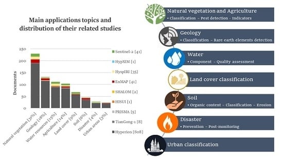
1. Introduction
Hyper- and multi-spectral technologies have both assisted remote sensing Earth Observation (EO) to stride forward in the past few decades. They developed gradually from meteorological projects to a multitude of other terrestrial applications [1]. Hyper- and multi-spectral sensors are based on the same physical technology. They both record radiance in the Visible to Near-InfraRed (VNIR) and Short-Wave InfraRed (SWIR) of the spectrum, VNIR spanning 400–1000 nm and SWIR 1000–2400 nm. Unlike multispectral sensors, such as Landsat-8 (11 bands), recording in a fairly limited number of discrete spectral bands (4–20 bands), hyperspectral sensors include a very large number of contiguous and narrow spectral bands of 5–15 nm [2]. Airborne hyperspectral sensors provide promising results for many applications as they combine a high spectral resolution with a high spatial resolution and are not so affected by atmospheric perturbation [3,4,5,6]. These platforms have played a key role in the development of hyperspectral science and applications [7,8,9]. Thanks to emblematic sensors such as HyMAP, Compact Airborne Spectrographic Imager (CASI), Airborne Visible/InfraRed Imaging Spectrometer (AVIRIS) , Digital Airborne Imaging Spectrometer (DAIS), Reflective Optics System Imaging Spectrometer (ROSIS), Airborne Imaging Spectrometer for Applications (AISA), Hyperspectral Digital Imagery Collection Experiment (HYDICE), Multispectral Infrared Visible Imaging Spectrometer (MIVIS), etc., hyperspectral research quickly expanded the number of hyperspectral applications in vegetation monitoring, water resources management, geology and land cover [9,10,11,12]. However, they do not allow regular and synoptic coverages over large areas as spaceborne sensors. Moreover, spaceborne sensors produce images with lower angular effects due to their much smaller field of view.
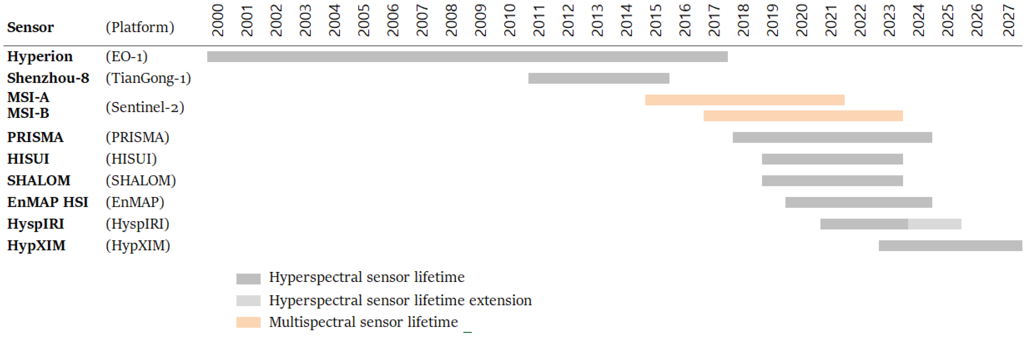
Despite the technological advances, hyperspectral satellites are still poorly represented in the spaceborne missions compared to multispectral ones, even considering forthcoming launches. Two hyperspectral missions for EO started around 2000 and were decisive in the progress of hyperspectral application development and demonstration. Hyperion (EO-1 platform) was first launched in 2000 and recorded data with a 30-m GSD and 400–2500 nm as the spectral range (Figure 1). Compact High Resolution Imaging Spectrometer (CHRIS) is fully programmable (i.e., in spatial resolution, total swath and spectral band settings) and provides five distinct angular views [13]. However, since this sensor does not cover the SWIR range, CHRIS was excluded from this hyperspectral application review. Several hyperspectral missions will shortly be launched, such as the PRISMA (PRecursore IperSpettrale della Missione Applicativa) Italian mission with a 30-m GSD and a wavelength range of 400–2505 nm [14], the EnMAP (Environmental Mapping and Analysis Program of 30-m GSD, 420–2500 nm) German mission [9] and the HISUI (Hyperspectral Imager SUIte of 30-m GSD, 400–2500) Japanese mission [15]. This low number of hyperspectral spaceborne instruments is mainly due to technical and practical constraints including challenging Signal-to-Noise Ratio (SNR) in particular bottom-of-atmosphere reflectance, sensor cost, data volume and associated data processing cost and time [10]. Several studies demonstrated the potential of hyperspectral sensors in a wide range of applications from geology [11], to vegetation [16,17], water resources [10,18] and land cover [19]. Each of these reviews focused on a very limited number of application subjects, missing a more comprehensive overview of hyperspectral remote sensing findings.
Hyperspectral imaging has proven its better discrimination than multispectral instruments thanks to its fine and continuous spectral information [20,21]. Concomitantly, the performance of multispectral technology is increasing gradually with the recent launch of new generation multispectral sensors. As part of the Copernicus program, the European Space Agency (ESA) developed a new EO mission with a high number of spectral bands; i.e., the Sentinel-2 (S2) constellation. Its main applications range from monitoring vegetation, geological component detection, as well as risk and disaster management [22]. Two identical S2 sensors covering the 443–2190-nm spectral range with 13 bands have been launched in 2015 and 2017 in order to provide unique multispectral reflectance time series over land and coastal zones. At least two other S2 sensors are planned to be launched from 2021 [23]. Their spatial and temporal resolutions reach 10, 20 and 60 m and five days of revisit time in the constellation mode. The S2 mission took advantage of previous hyperspectral sensors’ experiment and multispectral missions, such as MODIS (MODerate-resolution Imaging Spectroradiometer), Landsat, ALI (Advanced Land Imager), MERIS (MEdium Resolution Imaging Spectrometer) or SPOT (Satellites Pour l’Observation de la Terre), in order to identify the most suitable wavelengths enabling the observation of various geophysical variables.
In this EO context, this review specifically aims to survey hyperspectral remote sensing applications in order to best target hyperspectral potential and synergies with multispectral sensors, like S2. Therefore, this study encompasses the diversity of hyperspectral applications with a much broader perspective than previous works [10,11,16,17,18,19]. The specific objectives of this literature review of the results obtained based on spaceborne hyperspectral imagery are (i) to identify the main hyperspectral sensors and their applications compared to S2 and (ii) to identify the major limitations and advantages of current and future hyperspectral spaceborne sensors for operational EO.
2. Method
In order to assess the relevance of hyperspectral sensors in the S2 context, this section will first list and describe past and planned hyperspectral sensors for EO in the S2 context. The application literature of these sensors will then be analyzed to point out the most useful wavelengths that are not recorded by S2. This analysis will then help to discuss major current limitations and advantages of the hyperspectral sensors for operational EO applications. It should be noted that all information of this manuscript is adapted to the situation as of December 2017.
2.1. Review of Hyperspectral Sensors
As this study aims to target applications for hyperspectral sensors in the S2 context, this review focuses on EO spaceborne sensors with a ≤60-m resolution with a VNIR and SWIR capacity (i.e., from about 400–2400 nm). In order to select the appropriate sensors for our literature review, an inventory of the main spaceborne hyperspectral instruments has been indexed compiling their major specifications (e.g., satellite, swath width, spectrum range, number of spectral bands, spatial and temporal resolution, SNR, etc.). The information identified in this table is collected from publications, conference proceedings or websites found thanks to the Google and the Google Scholar platforms, using the words “hyperspectral”, the name of the sensor or the project and/or the name of a given specification. Military sensors and instruments with a non-EO objective were excluded from our research. Characteristics of S2 sensors were also added to the table to better compare respective specifications of multi- and hyper-spectral sensors.
2.2. Review of the Applications
After the identification of the main hyperspectral sensors, we extracted publications related to each hyperspectral sensor from the Scopus platform, using structured queries such as “SensorName AND hyperspectral” in titles, abstracts and keywords from January 1999–December 2016. However, because the name of the EnMAP sensor (i.e., Hyperspectral Imager) could be confused with other sensors, the “EnMAP AND hyperspectral” query was conducted instead. We applied the same methodology with S2 using the “Sentinel-2 AND multispectral” query. It is important to note that no further methodology was developed to detect other potential homonyms in our research. We also visualized the evolution of each sensor’s publications over time.
Then, we classified all of the identified articles, reviews and conference proceedings according to their main topic in order to select EO application research, except for the Hyperion sensor. Indeed, due to its very long lifetime, this hyperspectral sensor provided an abundant literature. Therefore, we decided to classify its 600 latest Scopus results only. Studies merely mentioning the sensor’s name in their title, abstract or keyword were also excluded. The analyzed publications have also been classified depending on the quality of their results: (a) results were satisfactory because the objectives were reached; (b) results were moderate at best seeing that the objectives were reached in part; (c) results were not satisfactory because the objectives were not reached.
2.3. Inventory of the Useful Wavelengths
We identified the most useful wavelengths for remote sensing applications mainly based on the studies of Segl et al. [24] and Miglani et al. [25]. Segl et al. [24] discussed the relevance of the multispectral bands of S2, and Miglani et al. [25] focused on the agricultural wavelengths. They were classified depending on their main application topic (vegetation, agriculture, soil, geology, water resources, disasters or land use). Note that vegetation, agriculture and land cover topics were merged, while disaster applications were mainly split into the vegetation applications (vegetation recovery after fire, wildfire assessment, etc.).
3. Results
3.1. Review of the Hyperspectral Sensors
A total of eight spaceborne hyperspectral sensors corresponding to the selected criteria have been identified (Table 1 and Table 2). Most of them are future sensors whose launches are planned after 2017 (i.e., PRISMA, EnMAP HyperSpectral Imager, HISUI, Spaceborne Hyperspectral Applicative Land and Ocean Mission (SHALOM) , Hyperspectral Infrared Imager (HyspIRI) and Hyperspectral X IMagery (HypXIM) (Figure 1). Two of them already have been decommissioned (i.e., Hyperion and TianGong-1 (TG-1)) (Figure 1). Their number of bands is about 200, except TianG-1 (i.e., 128), with a spectral resolution of approximately 10 nm. As a comparison, S2 sensors measure 13 spectral bands’ reflectance of 15–180 nm of spectral resolution depending on the band. It should be noted that several other EO hyperspectral sensors were identified; however, they did not fulfill our criteria or had a too restricted literature (see Appendix, Table A1 for a summary). Some of these sensors are planned to be launched soon and could offer alternative applications to the analyzed sensors.
3.2. Preliminary Analysis of the Literature Database
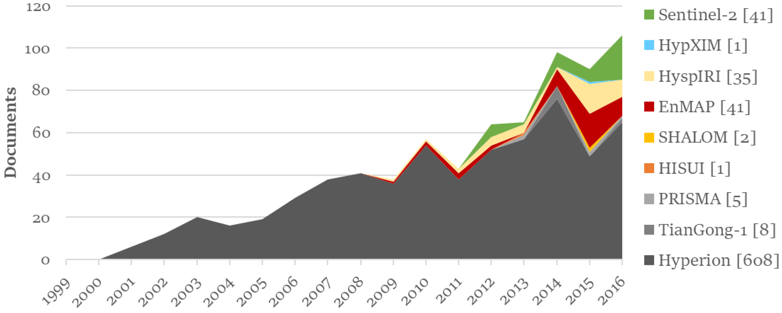
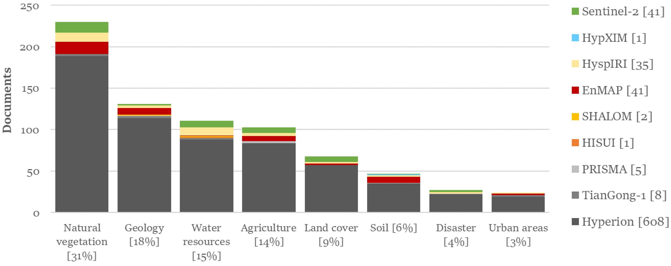
A total of 701 studies published between January 1999 and December 2016 focusing on hyperspectral applications was found for the eight selected sensors. The analysis of each of these hyperspectral sensors’ publications revealed that Hyperion and EnMAP clearly stood out from the crowd with a total of 608 and 41 publications, respectively (Table 1 and Table 2). S2 applications are covered by 41 studies. As shown by Figure 1 and Figure 2, the Hyperion sensor has been recording data for a long time period, leading to a particularly high and increasing number of publications throughout the years compared to the other sensors. In the last few years, the literature about the EnMAP and S2 missions clearly increased each year as their launch dates approached. However, due to the limited access to some of the papers and our restriction of Hyperion studies (i.e., selection of the 600 latest results), we analyzed a total of 175 EO-application publications (i.e., 78 for Hyperion, 2 for TG-1, 6 for PRISMA, 27 for EnMAP, 1 for HISUI, 1 for SHALOM, 32 for HyspIRI, 1 for HypXIM and 27 for S2; Table 3.
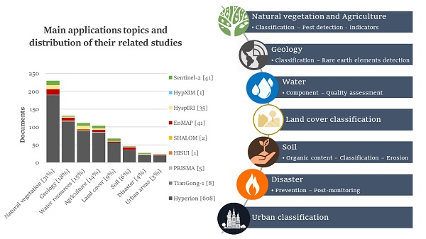
The literature has been classified into eight main topics: agriculture, geology, natural vegetation (not crops or grasslands), water resources, land cover, soil, disaster and urban areas (Figure 3). More than 30% of the total application studies were focused on natural vegetation, while agriculture and water resources represented around 15% of the hyperspectral research topics. Geological applications were the second most important subjects, representing around 18% of the documents. The proportions of publications related to land cover, soil, disaster and urban areas were quite similar (between 3% and 10%).
Table 3 shows the distribution of articles classified depending on the quality of their results. This table exclusively focuses on the analyzed studies and not on the total number of Scopus publications. Most of the S2 and EnMAP studies showed satisfactory results, reaching their objectives, while the Hyperion and HyspIRI results were much more distributed between satisfactory and moderate results. Nonetheless, the reader’s attention should be drawn to a potential bias of this classification. Indeed, we compared actual and simulated sensors results, seeing that some of them have not been launched yet.
3.3. Hyperspectral and Sentinel-2 Application Analysis
3.3.1. Natural and Agricultural Vegetation Applications
Because hyperspectral studies of agricultural and natural vegetation both regard plant analysis, their applications and conclusions are very similar. Three main kinds of vegetation applications have been identified in the literature: vegetation classification, pest detection and biophysical parameter estimation. All of them lead to more specific hyperspectral applications that will be described in this section.
• Vegetation Classification
The use of hyperspectral imagery has been demonstrated to be a cost-effective way for vegetation classification. Hyperspectral imaging allows the distinction of classes for various classification levels such as the forest type (fallow, primary forest, secondary forest, etc.) [36] or tree species [37]. For most of the forest classifications, the results were promising. Studies using simulated HyspIRI images were also able to map dominant species across varied ecosystems with fairly high overall accuracies [38,39] or to distinguish rangeland management practices [40]. The latter study compared the ability of HyspIRI for rangeland management identification with Landsat-8’s and S2’s. It highlighted that despite the better HyspIRI performances, S2 provided close results from the hyperspectral sensor and was identified as the best HyspIRI substitute in light of its characteristics (i.e., high spatial and temporal resolution, freely available data, etc.). Alongside this, Vaglio Laurin et al. [41] showed promising forest type classification results using simulated S2 images and highlighted the interest in LiDAR and optical data combination. However, they obtained better results with higher spatial and spectral resolution airborne hyperspectral images and therefore promoted coupling data from next generation hyperspectral sensors (e.g., EnMAP, HISUI, HyspIRI, PRISMA, etc.) with forest structure information. On the other hand, LiDAR and simulated HyspIRI data fusion provided moderate results for sparse shrub cover mapping, mainly because of the 60-m resolution of the hyperspectral sensor [42].
Hyperion classification could be used in heterogeneous contexts like savannas or mangroves. Discrimination of savanna vegetation physiognomies was achieved through the computation of Photosynthetic Vegetation (PV) fractional cover [37,43]. Such discrimination was possible thanks to differences of reflectance between the Near-InfraRed (NIR), corresponding to green cover fractions of the physiognomies, and the SWIR reflectance, corresponding to physiognomies with more Non-Photosynthetic Vegetation (NPV). On the other hand, the difficulty in distinguishing species belonging to the same family led to contrasted results for mangrove species classifications [44,45]. Corbane et al. [46] also estimated PV cover with various multispectral sensors and showed that S2 provided the best results in Mediterranean habitats, but due to its spatial resolution, highly fragmented patterns were not distinguished well. Analysis of Hyperion hyperspectral data has also been carried out to distinguish environmental gradients like gradual transition in vegetation [47]. They recommended a Support Vector Classification (SVC) model integrating synthetic mixtures with the parametrization to obtain more accurate results with the EnMAP sensor. Leitão et al. [48] performed a similar study and pointed out mapping precision enhancement with EnMAP data compared to Hyperion results. This difference in precision was associated with the better spatial coverage, revisit time, spectral and temporal resolution of EnMAP. Simulated EnMAP data also allowed good prediction of shrub cover showing gradients created by special agricultural management schemes in Portugal [49].
When classifying tropical tree species, care must be taken to select imagery at an appropriate time period. This period mainly depends on the phenological stages and on the species richness [50,51,52]. The necessity of taking the season into account was also noticed for agricultural studies [53]. For instance, Mariotto et al. [54] showed that the performance of hyperspectral data in discriminating crop types varied across the growing season depending on the growth stage of the crops. They obtained good results when discriminating up to five crops (cotton, maize, wheat, rice, alfalfa) taking into account this seasonal variability. They also showed that Hyperion and simulated HyspIRI outperformed multispectral sensors for crop classification and modeling of crop productivity.
Among the most frequent hyperspectral narrow bands used, 74% were located in the SWIR spectral range [54]. The significance of the SWIR in vegetation discrimination was also noticed in the study of Galvao et al. [55]. They used Vegetation Indices (VIs) sensitive to changes in chlorophyll, leaf water and lignin-cellulose content to differentiate five sugarcane varieties. The experiment was then reproduced to distinguish three soybean varieties using Hyperion images acquired from opposite off-nadir viewing directions, but similar solar geometry [56]. This study showed that higher average reflectance of the back scattering image produced better results than with forward scattering.
Reduction of data dimensionality has been demonstrated to also provide good classification results while reducing the processing time [36]. Moreover, the selection of the best Hyperspectral Narrow-Bands (HNBs) allows one to get rid of the Hughes phenomenon in the context of supervised classification using hyperspectral data. For example, Amato et al. [57] obtained close performances with a limited number of spectral bands, mainly spread on the VNIR PRISMA spectrum in order to classify agricultural land use. However, some studies have also demonstrated that SVC can overcome this phenomenon [58,59].
Vegetation classification represents thus a promising application for hyperspectral imaging in order to map simple landscapes (i.e., homogeneous zones, distinct species or legend levels). The higher spectral resolution of hyperspectral sensors compared to multispectral data clearly enhances vegetation application accuracy. For example, Hyperion outperformed Landsat when classifying crops, while they both have a 30-m GSD [60]. Thenkabail et al. [61] also concluded that Hyperion performed more accurate rainforest classification than ALI, IKONOS or ETM+. However, complex agroecosystems are much more challenging to classify for hyperspectral sensors because of their medium spatial resolution. The arrival of new hyperspectral sensors of high technology, such as the 30-m GSD EnMAP and HyspIRI sensors, should probably improve the accuracy of hyperspectral vegetation discrimination compared to Hyperion partly thanks to their higher SNR values and their better radiometric resolutions.
• Pest Detection and Mapping
Detecting agricultural and natural vegetation pests, such as invasive species or diseases, are other promising applications of hyperspectral remote sensing. Like species classification, invasive species detection requires images taken at an appropriate time. In order to distinguish invasive species from their environment, images taken at a contrasted senescence-time [62] should also show a distinct reflectance [63]. Indeed, similar spectral characteristics among the invasive species and their environment could represent a constraint for mapping [64]. Nonetheless, invasive species detection also requires pure pixels [64,65]. Therefore, the medium spatial resolution of Hyperion has been highlighted as a major drawback to detect invasive species organized on small patches or in linear arrangements [64,65].
Hyperspectral technology is also useful in order to detect crop diseases. Apan et al. [66] obtained a good classification accuracy with Hyperion when detecting orange rust disease in sugarcane crops. They underlined that the best indices allowing one to determine the affected sugarcane were those combining the VNIR bands with the 1660-nm band sensitive to moisture. White et al. [67] computed moisture indices derived from Hyperion data in order to detect insect damage. Indices with the largest correlation to the proportion of insect damage were those utilizing the SWIR and NIR regions of the spectrum concurrently. However, results were moderate at best (r = 0.51). Dutta et al. [68], obtained modest results with Hyperion when detecting disease in mustard crop. Samiappan et al. [69] were able to distinguish crop species at different stress levels with simulated HyspIRI data, but their study focused on the recognition of spectral signatures only. Simulated S2 red-edge bands provided good results when identifying coffee leaf rust infection levels in Zimbabwe [70]. Pest identification is thus a particular case of vegetation classification, but at a finer level of detection.
Spatial resolution is therefore the major constraint to overcome with hyperspectral sensors in order to apply pest or stress monitoring, and therefore precision agriculture. Indeed, the Hyperion sensor only outperformed the Landsat quantitative salinity stress estimation in the study of Hamzeh et al. [71], while Landsat outperformed Hyperion in categorical and quantitative estimations. However, at similar GSD, hyperspectral data could enhance invasive species detection compared to the multispectral sensor, e.g., Hyperion did better in detecting tamarisk invasive species compared to Landsat-5 thanks to its better spatial and radiometric resolutions [64]. Improving hyperspectral spatial resolution seems therefore essential to avoid mixed pixels. In order to do so, hyperspectral data in combination with better resolution data or with the use of multi-temporal series could increase the potential of hyperspectral data for pest detection applications.
• Biophysical Parameters’ Estimation
Besides vegetation identification and classification, many hyperspectral applications aimed at monitoring natural and agricultural vegetation through various biophysical parameters. However, seeing its potentialities, S2 has been predicted as an appropriate tool for vegetation parameter estimation [72].
Leaf Area Index (LAI) is one of the most estimated parameters with Hyperion. This sensor outperformed the ALI and ETM+ multispectral sensors for estimating LAI of coniferous forests [73]. EnMAP images resulted in accurate LAI estimations at the regional scale using a PROSAIL model with very close results to those obtained with the HySpex airborne sensor [74,75]. Siegmann et al. [75] pansharpened simulated EnMAP images with high resolution panchromatic imagery and with simulated S2 data. They showed that by reaching a finer spatial resolution, it significantly improved the prediction of wheat LAI. However, pansharpened images showed some artifacts in the resulting image. Moreover, pansharpened EnMAP with airborne aisaEAGLE data and spatially-enhanced EnMAP by fusion with S2 images led to a better LAI estimation. Nonetheless, this processing technique could be more complicated with real data. As a matter of fact, in this case, EnMAP, S2 and airborne images had the same acquisition conditions (i.e., date of acquisition, atmospheric conditions, etc.) because of the data simulation process. Richter et al. [76] also predicted LAI with S2 and EnMAP using radiative transfer models and inversion procedures. They demonstrated that S2 and EnMAP separately performed the best agricultural LAI estimations as compared to RapidEye and Landsat-5 sensors. The SWIR seems to be the best part of the spectrum to retrieve LAI with Hyperion due to spectral absorption features (pigments, water and other biochemicals) [77]. Other studies also pointed out the NIR when estimating LAI through VIs, but with questionable results [78]. Alongside this, red-edge bands (705 and 750 nm) showed promising results to test VIs for the estimation of LAI and also the chlorophyll content [79]. Wu et al. [79] demonstrated that it was possible to analyze the variation of these two parameters for different vegetation covers. However, three main drawbacks were underlined for an operational application. First, mixed pixels may lead to variation in the accuracy of certain indices depending on the species and the stress and nutritional levels. Furthermore, hyperspectral data are very sensitive to disturbances such as those from aerosols, branches and stems. Finally, relationships between spectral indices and biophysical variables are often species-specific, as explained in the Sims and Gamon [80] study.
However, determining the chlorophyll content at a species-specific scale with Hyperion data seems arduous mainly because of its medium spatial resolution [81], while S2 [82] and EnMAP [83] provide quite good results when estimating this parameter. Wu et al. [84] tested four VIs to estimate the canopy chlorophyll content of maize ranging from 100–1000 mg/m using Hyperion and Landsat Thematic Mapper images. They showed that the Green Chlorophyll (GC) index based on the green and the NIR bands was the best parameter for the interpretation of chlorophyll content in dense canopies.
The EnMAP sensor has also proven to assess Photochemical Reflectance Index (PRI) and Normalized Difference Vegetation Index (NDVI) accurately. Spectral and radiometric calibration uncertainties were beneath 1% considering the ±0.5-nm spectral stability of the sensor and were around 10% considering radiometric calibration [85]. Similarly, S2 also obtained encouraging results for estimating NDVI [82]. Huete et al. [86] derived coupled soil-plant biophysical parameters from Hyperion’s data to assess land conversion and degradation of a dryland in Argentina. They concluded that “greenness” measures, such as spectral VIs, were not well adapted to the assessment of land degradation and desertification in the context of the study. This was due to simultaneous changes in soil and vegetation optical properties leading to confusion when assessing the proportion of PV, NPV and of the soil background. They also pointed out that “greenness” was very sensitive to seasonal variations, as well as to species composition shifts.
Like the chlorophyll content, biomass is another challenging biophysical index for Hyperion in heterogeneous environments such as low vegetation cover areas [87,88]. The same observation was made for S2 data [89]. This difficulty was partially attributed to change in substrate reflectance beneath the canopy including soil and litter altering vegetation reflectance particularly for areas with low biomass. On the contrary, Sibanda et al. [40,90,91] were able to estimate biomass of grassland under different management practices with simulated S2 and HyspIRI data. Results with HyspIRI were slightly above those of S2 because of the higher spectral resolution and the narrower bandwidth of the hyperspectral sensor, but they both revealed comparable performances. Nonetheless, Hyperion data provided better results than multispectral sensors for discriminating between NPV and soil (i.e., ETM+ sensor) [88] or for estimating indices capturing the SWIR spectral region (i.e., OLI sensor) [87]. Agricultural studies also pointed out that Hyperion is useful to detect crop residues thanks to the SWIR region that is sensitive to lignin and cellulose [92,93].
Several studies with contrasted results were also dedicated to the mapping of foliar nitrogen content in forest. Despite good results in predicting nitrogen content of canopy based on Hyperion images, Townsend et al. [94] underlined the difficulty in designing a generalized analytical methodology. This was mainly due to substantial spectral variations caused by the canopy structure and species composition between study areas. On the contrary, the same method applied by McNeil et al. [95] was revealed to be inefficient to predict nitrogen content. HyspIRI seems to estimate nitrogen concentrations in cultivated grasslands correctly [38].
Water parameters, such as short- and long-term water stresses on deciduous forest communities, could also be retrieved [96]. Both simulated EnMAP and S2 data allowed a good estimation of drought indicators such as Moisture Stress Index (MSI), Chlorophyll Index (CI) and Simple Ratio (SR). This study highlighted EnMAP’s capacity to estimate the Photochemical Reflectance Index (PRI) despite its medium spatial resolution compared to S2, which could not assess it. However, synergic use of EnMAP and S2 data allowed considering directional effects (i.e., illumination angle). The EnMAP sensor is less sensitive to these effects when not operating in tilted mode in comparison with S2. The capacity of S2 to estimate evapotranspiration has been demonstrated by Ciraolo et al. [97], and it is suggested that precision farming could be an interesting application for the multispectral sensor.
Hyperion data can also be exploited to characterize forest structure such as the age and the height of the trees [98]. Ninck et al. [99] estimated forest spruce timber volumes with EnMAP and S2 images. Landsat-5 and SPOT 4 already allowed this estimation, but their fluctuating data acquisition frequency and data quality could cause a problem in terms of processing. However, results were not significantly different between EnMAP and S2 data, despite the higher spectral resolution of EnMAP. S2 sensor indeed retrieves red-edge spectral bands, which are highly relevant in terms of vegetation applications. The S2 sensor was also considered as more suitable for spectral unmixing forest crown components compared to EnMAP and airborne multispectral data [100]. S2 spectral bands were in fact selected to minimize noise and to focus on spectral bands that are the most useful for discriminating vegetation (i.e., red-edge bands).
Using simulated hyperspectral and thermal infrared HyspIRI data, Meerdink et al. [101] were able to accurately predict cellulose leaf level, lignin, leaf mass per area, nitrogen and water content parameters in Californian ecosystems. Similarly, Roberts et al. [102] predicted dominant plant species thanks to PV covers, and Marshall and Thenkabail [103] exposed encouraging results for crop biomass estimations.
To conclude, many studies demonstrated the hyperspectral sensors’ superiority for estimating vegetation indices (i.e., LAI, biomass, etc.) compared to multispectral data acquired at similar GSDs [40,73,77,87,88,90,91,99]. Moreover, enhanced hyperspectral data with higher spatial resolutions could further improve their estimation, such as the LAI prediction enhancement demonstrated by Siegmann et al. [75].
3.3.2. Geology Applications
The main geological application of hyperspectral sensors is surface composition mapping. The accuracy of geological maps is variable depending on the study and on the SNR quality of the sensor. Due to Hyperion’s low SNRs in the SWIR, Kruse et al. [104] concluded that only basic mineralogical information can be extracted from Hyperion data for a complex geologic system. They showed that the AVIRIS airborne hyperspectral sensor outperformed Hyperion for geological mapping due to SNR differences (approximately 50:1 in the SWIR for Hyperion versus more than 500:1 for AVIRIS). Similarly, ALI+ and ASTER multispectral sensors, used for geological exploration, mapped minerals almost as well as Hyperion as a result of their good SNRs (respectively 140:1–180:1 and 231:1–466:1 for the SWIR bands) [105]. However, none of those sensors were relevant for mapping the diverse range of surface materials exposed in the studied area. Moreover, a comparison of ASTER and Hyperion in a hyperarid desert region showed that both sensors discriminated similar surface types, but that ASTER allowed a more detailed classification of the surface composition [106]. Hyperion’s data were found of greater utility than data from the broad bands Landsat TM to create surface cover abundance maps [107,108]. Some Hyperion studies were able to distinguish green vegetation from talc, dolomite, chlorite and white micas [109], while others differentiated calcite from dolomite [7], detected differences in solid solution of micas [7] or spotted ammonium-bearing minerals with the 1558-nm band characterized by a relatively high SNR [110]. On the other hand, Leverington [107,108] obtained poor to moderate results when using Hyperion to separate several important sedimentary lithological end-members in Texas and Canada. They pointed out the low SNR as a critical factor. Distinguishing calcite from dolomite with TG-1 data was difficult while zoisite, mica, quartz, alunite, cummingtontie , sodalite, dolomite, anorthite and actinolite were successfully discriminated [111].
Geological classification not only depends on the SNR sensor characteristics, but also on the image conditions of acquisition (i.e., sun illumination, concentration levels of minerals, extend of minerals, season, exposition of the geology) [7,112,113]. Hyperion capacity for mine waste monitoring was evaluated by Mielke et al. [114]. They pointed out the critical revisit time of Hyperion and suggested to combine hyperspectral data for mine waste identification with multispectral data such as S2 for repetitive area-wide mapping. The wide spectral range of hyperspectral sensors appeared to be a good advantage for geological applications. However, their medium spatial resolution and the low SNR values in the SWIR made it sometimes difficult.
Mielke et al. [115] compared results of Hyperion, the multispectral Operational Land Imager (OLI) sensor, ALI, ASTER, ETM+, EnMAP and S2 for mine waste monitoring. EnMAP provided the best overall accuracies for mapping gold mining material, pyroxene proxies for platinum and other iron absorption feature of mineral linked to mine waste. S2 was then the second best data for mapping of gold mines. However, S2 could not distinguish surface mineralogy correctly, unlike EnMAP. In another study, Mielke et al. [116] showed that simulated EnMAP data provided better results than Hyperion in order to characterize mineral deposits and to highlight exploration anomalies (i.e., unexpected soil properties, which are indicators of valuable soil elements). They implemented an algorithm and expert system (EnGeoMAP, the EnMAP Geological Mapper ) to detect metal sulfide mineral deposit sites. Instead of EnGeoMAP, Bösche [113] implemented another methodology called Rare Earth Elements MAPping (REEMAP) to detect rare Earth elements and oxides (e.g., erbium, neodymium, dysprosium, holmium, samarium, europium and thulium) with EnMAP. However, like other research, this paper highlighted some limitations such as the inadequate EnMAP spatial resolution to map rare mineral dykes. The combined analysis of remote sensing data with field works is therefore necessary. However, despite medium spatial resolution, discrimination of mafic and ultramafic rock units was feasible at a broad scale with simulated EnMAP images [117].
The coarse resolution of HyspIRI (60-m GSD) was also pointed out as a limitation to detect occurrences and details of surface characteristics [118,119]. However, these studies demonstrated that HyspIRI could accurately map geologic materials associated with hydrothermal systems (e.g., goethite, hematite, jarosite, alunite, kaolinite, dickite, muscovite-illite, montmorillonite, calcite, buddingtonite and hydrothermal silica). Moreover, simulated HyspIRI data were also able to successfully map epidote, muscovite and kaolinite combining SWIR and Thermal InfraRed (TIR) bands [34].
Geological applications are therefore suitable applications for hyperspectral sensors enabling an identical or better discrimination of the potential geological components than multispectral sensors of similar GSD [107,108,120]. However, the SNR value is identified as the hyperspectral critical factor for geological applications, and a higher spatial resolution is required only, but for finer detection (such as mineral dykes detection). This is why Yokoya et al. [121] fused EnMAP and S2 data to enhance the hyperspectral GSD of the sensor and demonstrated the efficiency of their synergistic use.
3.3.3. Soil Applications
Papers dedicated to soils were limited, representing only 6% of all the hyperspectral publications and 2.5% of the S2’s (Figure 3). Most of them focused on the soil chemical properties’ detection, and only moderate results have been reported. For estimating soil salinity content with Hyperion in the Yellow River delta in China, Weng et al. [122] constructed an index based on field spectrometer measurements. The soil salinity index was calculated based on two specific SWIR bands leading to a quantitative salinity map with moderate accuracy. Gomez et al. and Weng et al. [5,122] both mapped the Soil Organic Content (SOC) with Hyperion images and compared the results with field spectrometer measures. Gomez et al. [5] attributed the lower accuracy to two factors: the noise in the Hyperion spectra and the medium spatial resolution concealing the spectral features of soil organic matter. Other studies mapping soil carbon content also obtained contrasted results and attributed the low accuracy prediction to the spatial resolution of Hyperion [3] or EnMAP [6]. Steinberg et al. [6] predicted organic carbon content, but also mapped other soil properties such as clay and iron oxides’ content with simulated EnMAP images. Maps derived from EnMAP data showed a lower accuracy than the better spatial resolution HyMAP hyperspectral images. However, this medium spatial resolution seems to be appropriate for regional-scale soil predictions [6,122]. On the other hand, comparison of soil texture (i.e., clay, sand, silt) and SOC estimations with Hyperion, HyspIRI, EnMAP, PRISMA, Landsat-8, ALI and S2 data showed that forthcoming hyperspectral sensors (i.e., HyspIRI, EnMAP and PRISMA) provided quite similar results [123]. Moreover, these forthcoming sensors presented better overall accuracies than the other sensors (i.e., Hyperion, Landsat-8 and S2) due to their higher number of spectral bands and their narrower bandwidths. Castaldi et al. [124] predicted soil clay content (e.g., kaolinite, montmorillonite, illite) by taking into account soil moisture information based on PRISMA data, but obtained moderate results. Like Steinberg et al. [6], Lu et al. [3] predicted SOC, but also other soil properties, such as total phosphorus content, pH and cation exchange capacity and obtained moderate accuracy. Furthermore, clay content could be accurately predicted with data from 5–30-m spatial resolution, such as SHALOM, PRISMA, EnMAP, HyspIRI and HypXIM images [125].
Hyperspectral sensors have also been used for erosion mapping. However, the spatial resolution of EnMAP was pointed out as a limiting factor in order to map land use cover related to soil erosion (e.g., PV, NPV and bare soils) [126]. Nonetheless, this sensor seemed adequate for regional-scale studies of erosion. The EnMAP capacity of short- and long-term change monitoring also represented an advantage to model erosion caused by seasonal variations, by short- and mid-term decisions, or by climate impacts in the long term.
Spatial resolution seems thus to be once again the Achilles heel of hyperspectral sensors to retrieve soil parameters at a fine scale. However, hyperspectral sensors are still providing more useful information than multispectral data acquired at the same GSD, such as for the soil texture or SOC estimation [123].
3.3.4. Land Cover Applications
Land cover applications showed contrasting results depending on their respective objectives. The monitoring of changes in vegetation is particularly useful for land degradation assessment [86]. Petropolous et al. [127] emphasized the relevance of Hyperion imagery for mapping and monitoring land degradation and desertification. They showed the performance of Hyperion data for land use classification in Mediterranean environments. However, despite a good overall accuracy, some classes were more difficult to identify, such as sparsely-vegetated areas, heterogeneous agricultural areas, burnt areas or transition between land uses. Ben-Arfa et al. [128] used Hyperion imagery for mapping oases dynamics caused by competition for land and water between different user groups in the Gabes area in Tunisia. They emphasized the efficiency of the cellulose index, vegetation mask and water presence index for the discrimination of land use. They also showed that spectral unmixing was sensitive to slight ground changes. Xu and Gong [129] compared the capacity of Hyperion with the multispectral ALI sensor to discriminate different land use and land cover in California. They showed that overall, Hyperion did not produce significantly better results than ALI. However, for various dry grass vegetation classes and impervious land use categories (new residential lots), Hyperion data produced better results than ALI data.
Simulated S2 data provided satisfactory results for land cover mapping using SVC classifier in order to discriminate seven classes with 10 spectral bands [130]. The S2 revisit time, as well as its fine spatial, spectral and radiometric resolutions, was pointed out in the studies of Törmä et al. [131,132] as well-suited for land cover classification. These characteristics could help for example to better distinguish meadows from other agricultural land uses. The multispectral sensor allowed them to improve the CORINE Land Cover classification. Simulated HyspIRI images also improved land cover mapping with its short revisit time and have resulted in a better land cover map than S2, or Landsat-8 data [133,134]. Indeed, this hyperspectral sensor can target key spectral features related to specific physical and chemical characteristics. Hunger et al. [135] combined Sentinel-1 SAR with S2 multispectral bands to classify land cover and showed that this method does not always improve the classification accuracy.
Therefore, while the medium spatial resolution of hyperspectral sensors is here again pointed out, their high number of bands with fine bandwidths are real assets compared to S2 or to multispectral sensors with similar GSD for land cover applications. However, it will still be difficult to classify landscape heterogeneity and complexity at 30-m GSD. Fusing hyperspectral and multispectral data, Hyperion and IKONOS, increases the classification accuracy of scattered and irregular areas [136].
3.3.5. Urban Applications
Regarding urban applications, classification of impervious surface types was one of the major concerns in the hyperspectral literature. Some studies reported successful mapping of urban areas, showing better results with Hyperion images than the ALI multispectral sensor to discern low-albedo surface materials (i.e., asphalt). This was mainly due to its higher number of spectral bands in the mid-infrared region [21]. Others demonstrated better results with Hyperion than with Landsat data in classifying non-impervious material, construction concrete (mainly larger buildings, industrial/commercial areas), asphaltic concrete (mainly parking lots) and paving asphalt (mainly roads) [137]. Furthermore, Hyperion showed better results than the ETM+ and ALI sensors to retrieve complex urban land cover, like in Venice [138]. However, Hyperion was not able to discriminate land cover complexity. Only three main urban covers were indeed identified, including vegetation, paving and roofing, while better results were observed when using MIVIS airborne hyperspectral data of higher spatial resolution.
Okujeni et al. [139] quantified land cover on an urban gradient with simulated EnMAP data. However, its medium spatial resolution was a source of important spatial detail loss and of a significant mixed pixels increase compared with hyperspectral airborne sensors. Therefore, material discrimination was difficult, especially for classes with high spectral similarities. For example, roof detection seemed to be more sensitive to spatial resolution than pavement or trees. This highlights the importance of high spectral resolution data acquired at high spatial resolution in heterogeneous urban areas. Nonetheless, compared to Landsat ETM (30-m GSD), EnMAP (30-m GSD) allowed a better impervious surface mapping [139]. However, compared to the airborne HyMAP (9-m GSD), the EnMAP medium spatial resolution induced a loss of detail and more mixed pixels, reducing the mapping accuracy of heterogeneous and complex areas. On the other hand, Heldens et al. [140] noted that EnMAP could improve the within-class discrimination for impervious surfaces.
A review focusing on hyperspectral urban applications identified four frequently-addressed urban topics (i.e., development and planning, growth assessment, risk and vulnerability assessment and climate) [140]. It emphasized that a large number of studies made a successful use of medium spatial resolution data (≥30 m) in the field of urban planning and development and urban growth assessment. However, for urban climate analysis and structure parameters, they underlined the discrepancy between the average size of urban objects and the EnMAP spatial resolution. They concluded that research is needed to resolve the spectral composition of a pixel in order to fully exploit spectral information content. Moreover, the use of image fusion techniques or the use of complementary information such as thermal properties of the targets could lead to further improvements. To this end, Roberts et al. [141] improved the urban environment discrimination taking advantage of the synergy between Visible to Short Wavelength InfraRed (VSWIR) and TIR HyspIRI data. However, the HyspIRI data are at 60-m GSD, and they noted the poor results for non-extensive material mapping (e.g., industrial rooftops, parks, urban forests, open fields, etc.). The better spatial resolution of the hyperspectral TG-1 sensor (10 m in the VNIR and 20 m in the SWIR) is reported to have a higher classification accuracy in the heterogeneous environment of Beijing than with Hyperion [142].
Same as for land cover applications, the hyperspectral spatial resolution is identified as the main constraint for understanding the urban landscape complexity while their high spectral resolution allows distinguishing various surfaces. While many studies indeed identified hyperspectral sensors as the best data source for urban classification [21,137,138,139], they also highlighted the necessity of higher spatial resolution.
3.3.6. Water Resource Applications
Most of the analyzed studies dealing with water resources focused on quality assessment [18,143] and component classification [144,145,146]. Hyperion coastal water quality assessment emphasized the need for a continuous coverage of an approximately 10–12-nm bandwidth to capture some variables such as the cyano-phycoerythrin, useful for toxic algae detection [18]. Moreover, Giardino et al. [143] obtained moderate results when assessing the water quality with Hyperion of the Garda Lake in Italy. The assessment of colored dissolved organic matter was not achievable due to its low concentration in the lake. Their results were satisfactory for chlorophyll-a, while they were moderate at best for the tripton that sedimented in the lake. The ability of Hyperion, CHRIS/Proba and HyspIRI to detect phycocyanin concentrations through chlorophyll-a content was evaluated in the study of Ogashawara et al. [146]. This study revealed the higher sensitivity of CHRIS to chlorophyll-a concentrations. On the other hand, better results were obtained in classifying seagrass types with Hyperion images than with the ALI and Thematic Mapper sensors [144]. Probably hampered by the high flood period, another study reported only moderate results in modeling water constituents of the Amazon River with Hyperion [147]. This sensor also retrieved better seagrass biometric parameters (i.e., submerged aquatic vegetation cover, LAI and biomass). Studies accurately predicted bathymetry from 1–25 m deep with Hyperion images [148].
Devred et al. [149] reviewed the water resource applications of the HyspIRI sensor, such as water quality, species succession in estuaries, nutrients loads and changes in fisheries. Its spatial and spectral resolutions represent good advantages for water studies. Some studies showed that this sensor is also able to evaluate chlorophyll-a, phycocyanin and to follow giant kelp dynamics or Sargassum macroalgae, while algal bloom dynamics and ecosystem responses analysis are more difficult [150,151,152]. HyspIRI has been shown to be able to map cyanobacterial blooms if the image was taken on the optimal day [149,153]. However, the 19-day revisit time of the forthcoming hyperspectral sensor would probably limit this application. According to Palacios et al. [154], quality calibration, sensor sensitivity and atmospheric correction improvements of HyspIRI are required to detect chlorophyll-a. Turpie et al. [155] introduced this sensor as one of the few missions to observe fine-scale structure in coastal wetlands. This sensor can therefore help to study coastal environment, properties, biochemical cycling and water quality. Moreover, supported by its TIR sensor, HyspIRI would also be able to follow hydrologic and hydrometeorological processes.
Xi et al. [145] concluded that phytoplankton discrimination accuracy with EnMAP was highly variable and influenced by the chlorophyll content in the water. Chlorophyll content estimation depended mainly on pure water absorption for chlorophyll concentrations under 1 mg/m. Phytoplankton monitoring using EnMAP data could thus turn out to be inappropriate. Furthermore, few phytoplankton taxonomic groups were distinguished because of their highly similar reflectances.
After natural vegetation, most of the S2 studies we have analyzed focused on water resources (Figure 3). Some were able to detect cyanobacterial blooms [156,157]; other studies mapped water bodies [158] or estimated chlorophyll-a contents [159]. The latter showed that S2 has the ideal combination of spectral and spatial resolutions for small inland water bodies compared to WorldView-2, Landsat-8, MODIS and Sentinel-3 [159]. Moreover, its frequent revisiting time enabled S2 to describe effectively the dynamics of Planktothrix rubescens contaminated water [160]. A few days (up to a week’s time) between the field work of taking water samples and S2 acquisition of the lake chlorophyll-a content does not affect the accuracy of the chlorophyll map [157]. However, a 30-m GSD was not precise enough to represent the cyanobacterial bloom spatial variability. The study of Hedley et al. [161] indicated that S2 was able to discriminate reef benthic composition thanks to its fine bandwidths, its high spatial resolution and its additional 443-nm band. Nonetheless, it could not differentiate coral mortality or algal cover, unlike HISUI [162]. Moreover, S2 is a land monitoring mission that covers tropical waters within 20 km from coasts, limiting therefore potential coral reef applications.
Hyperspectral spatial and spectral resolutions thus seem to be appropriate for water resources applications. However, their temporal resolution is now their major constraint for water quality monitoring. Seeing that S2 provides a five-day revisit time and due to its medium spectral resolution, the advantage could be to combine both types of sensors.
3.3.7. Disaster Applications
The hyperspectral literature mainly focused on disaster prevention and post-monitoring, while their critical revisit time prevents systematic monitoring, such as volcanic eruption follow-up [163]. Ustin et al. [164], Yoon and Kim [165] and Roberts et al. [166] tried to predict fire danger in California and Korea with Hyperion data. They obtained contradictory results in distinguishing green vegetation from dry plant litter and bare soil. Failures in preventing wildfire were therefore attributed to low Hyperion SNR in the SWIR, reducing its capacity to estimate canopy water content [164]. On the contrary, Roberts et al. [166] and Yoon and Kim [165] underlined the ability of Hyperion to resolve ligno-cellulose bands and thus detect fire danger areas despite its low SNR. Hunt et al. [167] also tried to estimate fuel moisture content with HyspIRI data, but showed that the sensor’s revisit time will not be sufficient to monitor fire. Identification of debris flow areas represents another hyperspectral application. By integrating information on slope, Crowley et al. [168] obtained satisfactory results in detecting hydrothermally-altered rocks contributing to the avalanches and identified the most risky areas. Brown et al. [169] successfully predicted the larval mosquito (Anopheles punctipennis) presence that was positively correlated with the maximum Disease Water Stress Index (DWSI) and negatively correlated with the maximum Carter Miller Stress Index (CMSI), the minimum Normalized Difference Vegetation Index (NDVI) and the maximum Normalized Difference Water Index (NDWI).
Post-disaster applications with Hyperion data showed high overall accuracies when monitoring post-fire vegetation degradation [170] and recovery [171]. S2 red-edge bands also allowed discriminating burn severities in Mediterranean forest ecosystems accurately [172]. A study about the influence of spatial resolution on fire detection showed that the 60-m HyspIRI resolution generally overestimates fire surfaces and underestimates temperatures compared to higher resolution hyperspectral data [173]. Arellano et al. [174] studied the effect of hydrocarbon pollution in the Amazon forest using Hyperion. They concluded that tropical forests exposed to hydrocarbon pollution showed reduced levels of chlorophyll content, higher levels of foliar water content and leaf structural changes that can be stressed by VIs extracted from Hyperion narrow bands. PRISMA is another potential tool for post-disaster management in detecting and identifying natural and anthropic disaster on vegetation [175].
The revisit time of hyperspectral sensors and low SNRs in the SWIR of Hyperion thus mainly limit disaster monitoring and fire prevention applications.
4. Discussion
4.1. Inventory of the Useful Wavelengths
The most useful wavelengths for remote sensing applications were mainly identified based on the publications of Thenkabail et al. [16] and of Segl et al. [24]. Segl et al. [24] discussed the relevance of the S2 bands, while many others reviewed the use of hyperspectral data for agricultural and vegetation applications. Wavelengths were classified depending on their main applications (Figure 4 and Figure 5). No information about useful bands was available for land use applications. Except for water resources, all applications required bands spread on the full 400–2500 nm spectrum. The ranges of the wavelengths used for geology, soil, water resources and agriculture/vegetation/land cover applications were respectively 430–2340 nm, 440–2203 nm, 413–758 nm and 420–2385 nm. The agricultural, vegetation and land cover applications are the ones using the greatest number of wavelengths. Despite its wide spectrum and its high band number, many useful wavebands are not covered by S2, and most of them are dedicated to vegetation applications only.
Regarding geological applications, most bands were located in the SWIR. Some authors indicated the importance of the 2000–2400-nm bands for geological applications to detect components such as clays, calcite, dolomite, quartzite or kaolinite [7,112,113,115]. Bands from 430 nm–900 nm were pointed out as diagnostic for ferric iron [112,115]. Many wavelengths were also identified as useful for vegetation studies. The VNIR wavelengths were mainly used for computing VIs related to biomass or greenness. The wavelengths around 2100–2400 nm were useful for the assessment of lignin, cellulose and water content, while those around 1600 nm were identified as useful for some disease detection [66,68]. Regarding soil applications, bands located in the VNIR were mainly used for organic matter identification, as well as bands located around 1100 nm. Bands around 2000–2200 nm were used for soil salinity assessment. For water applications, most VNIR bands were used to identify vegetation, phytoplankton or algal cells. The 440-nm band was identified as useful to identify dissolved organic matter [143].
Figure 5 depicts the 28 HNBs identified as non-redundant by Thenkabail et al. [16] and the 26 HNBs identified as optimal by Miglani et al. [25] for retrieving crops and vegetation biophysical parameters. Based on one Hyperion scene, Miglani et al. [25] concluded that among the 242 HNBs of Hyperion, 26 were optimal for monitoring wheat, sugarcane, potato, mustard, berseem and sorghum with high accuracy. Sixteen HNBs were located in the VNIR (mainly for detecting chlorophyll, biomass and stressed vegetation), and 10 were located in the SWIR (mainly for LAI, biomass and moisture detection). Based on two Hyperion scenes and other surface hyperspectral data, Thenkabail et al. [176] tried to determine the optimal HNBs for the eight leading worldwide crops (wheat, corn, rice, barley, soybeans, pulses, cotton and alfalfa). They integrated data collected during six distinct growth stages and from multiple study areas in various worldwide agroecosystems of Africa, Middle East, Central Asia and India from over 100 research papers [177] in order to get robust regional results. The eight crops were described and classified using 20 HNBs with a very high accuracy, providing better results than the multispectral ETM+ or ALI sensors. Bands were equally distributed between the VNIR and the SWIR. They also concluded that 33 optimal HNBs and an equal number of hyperspectral VIs were sufficient to model and study specific biophysical and biochemical properties of the main crops of the world. Those biophysical indices were related to biomass, LAI, plant density yield, carotenoids, anthocyanin, chlorophyll, plant stress indices, plant water and moisture indices, light use efficiency or the lignin-cellulose-residue index. Among the best 33 HNBs, 17 were located in the SWIR. These studies therefore illustrate the possibility of using hyperspectral sensors to select an optimal subset of bands according to each application in order to create new multispectral sensors (such as ENVISAT/MERIS and now Sentinel-3/OLCI).
In light of these two figures, many specific bands of hyperspectral applications could not be covered by the S2 sensors, mainly those concerning agriculture and natural vegetation. Indeed, S2 shows an important gap between Band 9 (945 nm; dedicated to water vapor assessment) and Band 10 (1375 nm; dedicated to cirrus assessment). This gap covers wavelengths that are useful for the estimation of water, moisture, biomass, biophysical and biochemical quantities (e.g., plant height, crop type, total chlorophyll, etc.), water sensitivity and LAI [16,25]. The other gap between Bands 11 (1614 nm) and 12 (2202 nm) covers some applications such as cellulose, lignin, starch or biomass detection. Even if S2 estimated biomass quite well [40,89,91], we could expect a better estimation if the multispectral sensor covered these spectral ranges.
4.2. Limitations of the Hyperspectral Sensors Specifications
Table 4 summarizes the requirements of the groups of applications in terms of spatial and temporal resolutions. Hyperion and future sensors such as PRISMA, EnMap, HyspIRI or HISUI have a great potential for applications with a medium spatial resolution and a medium revisit time (Table 1 and Table 2). SHALOM has a medium to high spatial resolution and a high revisit time, while HypXIM has high spatial and temporal resolutions.
4.2.1. Spatial Resolution
The spatial resolution of future spaceborne hyperspectral missions at 30-m GSD has been considered as a major drawback for some applications, while S2 provides images from 10–20-m spatial resolution. This spatial resolution difference between multi- and hyper-spectral images primarily comes from the technical trade-off between spectral and spatial resolutions. A 30-m spatial resolution mainly affected the reviewed literature about vegetation, soil, geology, land use, urban and disaster monitoring topics (Table 4). Several studies for vegetation classification have reported hyperspectral GSD as a major limiting factor [64,65,75,117,126,127,140,178,179]. The medium spatial resolution of these sensors results in images with mixed-pixels, which highly affects classification and detection performances [180]. Eckert and Kneubülher [53] and Okujeni et al. [139] underlined this phenomenon in a small-spaced pattern of many fields in Switzerland and of a complex urban gradient of Germany, causing a decrease of classification accuracy. The mixed surfaces produced by the 30-m spatial resolution of Hyperion were also pointed out to explain the poor results obtained by Gomez et al. [5], Lu et al. [3] and Steinberg et al. [6] when mapping soil organic matter. According to Carter et al. [64], the within-pixel spectral mixing reduces the benefits of its high spectral resolution and leads to a decrease of the classification accuracy. They showed that only ground plots containing 80–100% of invasive species coverage were of sufficient size to yield 30-m GSD reference pixels. Walsh et al. [181] overcame the mixing problem induced by this low GSD by merging Hyperion images with QuickBird multispectral data. This process took advantage of the spatial and spectral resolutions of each data source to differentiate challenging cover classes and enabled good results. Another way of reducing this spatial resolution problem involves a multi-temporal unmixing, such as taking into account spectral features extracted from different seasons [182].
Other studies highlighted that 30 m is larger than some objects of interest such as invasive plants [64,65], rare earth elements [113] or complex land cover [138,140]. However, some authors successfully used image fusion techniques in order to overcome the medium spatial resolution of Hyperion as Walsh et al. [181] mapping invasive species of guava and Siegmann et al. [75] using pansharpened EnMAP images with simulated S2 data to predict LAI. The combined EnMAP and S2 data retrieved better results than using either hyper- or multispectral data separately. Even with a better point spread function (i.e., a lower sensor blur), the 30-m resolution of most hyperspectral sensors (Hyperion, PRISMA, HISUI, EnMAP, HyspIRI) is a limiting factor especially for highly heterogeneous environments (fragmented ecosystem, mosaic of land cover or land use) or for targets with small densities (some vegetation species, arid environment, residues, dry vegetation, etc.). Small targets such as urban areas are also difficult to identify [140], while finer resolution sensors (i.e., TG-1 of 10-m GSD) provided encouraging results for mapping complex urban land cover [142]. For these reasons, the even coarser HyspIRI GSD of 60 m was pointed out by many studies [42,101,118,119,123,125,152,183,184] and was therefore recently reduced to reach 30 m [34,155]. However, this reduction may not be adequate enough to study small and patchy areas such as coastal wetlands [155].
Spatial resolutions of most actual and future hyperspectral sensors result therefore in a significant limitation of the number of applications. On the other hand, some applications require medium spatial resolution. For example, despite its 10-m resolution, fine-scale vegetation patterns were hardly distinguished by S2, while their general organization across habitats was better mapped [185]. Moreover, the modeling of the above-ground carbon stock of mangroves showed low accuracies when using fine spatial resolution images, while the results using Hyperion data were good [186]. The suitable spatial resolution of an hyperspectral image thus depends on the specific application, and therefore on the target. Crop disease detection requires much higher spatial resolution (around 5 m) than crop type mapping (10–30 m) (Table 4). Moreover, it also depends on the specific characteristics of the study area. For example, spatial resolution has to be selected based on the targeted agroecosystem (e.g., U.S. fields are much larger and homogeneous than Madagascar’s), city, etc. No generic spatial resolution suggestion could therefore be proposed, and a baseline field-knowledge seems required to properly select the most suitable sensor.
Two forthcoming hyperspectral sensors, PRISMA and HypXIM, will capture Earth images at the same time with higher resolution panchromatic sensors [14,35]. The resolution of the panchromatic band for PRISMA and HypXIM will be 5 m and 2 m, respectively. They can be used to pansharpen the respective sensor data. Furthermore, S2 provides freely available and global high spatial resolution images with a frequent revisit time. This would probably pave the way toward new hyperspectral-spatially-improved application studies. Indeed, many spatial-enhancement methods have been proposed for hyperspectral data [121,187,188,189]. For example, Yokoya et al. [121] succeeded in improving the GSD of simulated EnMAP images with simulated S2 data. This study fused both data using a matrix factorization method to end up with a 10-m resolution EnMAP image that showed great potential for mineral mapping. Other studies developed a more generic spatial-enhancement method to combine hyperspectral and multispectral data, such as Ghasrodashti et al. [189], who used a new spectral unmixing and a Bayesian sparse representation, to obtain a significant spatial enhancement. The fusion method of Yang et al. [190] also showed encouraging results with a pixel group based the non-local sparse representation method, like the sparse non-negative matrix factorization technique [191]. For further details, see the review of Loncan et al. [187], which compared the main hyperspectral-multispectral pansharpening methods and identified their pros and cons (i.e., fusion performances, computational costs, etc.).
4.2.2. Revisit Time
Revisit time is rarely taken into account in the considered literature. However, it is a crucial parameter to determine potential applications for a sensor. With a revisiting capacity higher than 15 days, except in tilted mode (Table 1 and Table 2) and HypXIM, previous and planned hyperspectral sensors are not designed for applications requiring a high revisit frequency, unless reducing their revisit time by using them in a constellation mode. Moreover, the gap between revisiting capabilities and actual usable data availability also has to be taken into account due to atmospheric and aerosol perturbations. Phenomena with no major variation within 15 days or more could thus represent relevant applications. This excludes crop, vegetation and disaster monitoring or disaster prevention (Table 4). However, post-disaster monitoring such as vegetation recovery after fire or pollution events is possible [170]. In bare areas, this revisit time allows geological applications, as well as applications related to the assessment of soil properties. Vegetation classification, determination of land cover or land use are also possible if images are available every 15 days. Water resources applications are relevant regarding bathymetry, assessment of water quality or classification of coastal ecosystems, but not regarding monitoring of phenomena such as algal bloom or water pollution. Another solution to reduce revisit time is to modify the View Zenith Angle (VZA), like EnMAP and SHALOM. However, this negatively affects the spatial resolution and consequently, the resulting information is probably less consistent due to the variable pixel footprint.
Another way to mitigate the revisit time of forthcoming hyperspectral sensors is to utilize them in a constellation mode. Hyperspectral sensors would then be more relevant for the assessment of wildfire danger or for crop monitoring [78,164]. However, those sensors can be used to prevent other disasters where revisit time is not a limiting factor, such as the identification of areas with a high risk of landslides [168]. Post-disaster assessment also does not require a frequent revisit such as vegetation recovery after fire or pollution events, which can also be characterized based on the hyperspectral sensors [171,174]. Applications in the field of water resources such as bathymetry studies or assessment of water quality seem to be globally relevant, but frequent surveys for water pollution or algal bloom are not possible with only one spacecraft [18,143,148]. Another solution to alleviate the constraint of revisit time could be to combine the high temporal survey capacity of S2 or panchromatic sensors with the high spectral information of the hyperspectral sensors through pansharpening.
4.2.3. Signal-To-Noise Ratios in the SWIR for Hyperion
Because of their narrow bands, hyperspectral sensors measure lower SNRs than multispectral instruments [123]. Moreover, the low solar irradiance in the SWIR significantly reduces the SNR values in this part of the hyperspectral spectrum. A few months after the launch of Hyperion, Pearlman et al. [193] reported SNRs values from 140:1–190:1 in the VNIR, 96:1 in the SWIR around 1225 nm and 38:1 in the SWIR around 2125 nm. Based on Hyperion imagery and three specific targets when mapping hydrothermally-altered rocks, Gersman et al. [110] estimated an SNR of 90:1 for the VIS range, 60:1 for the 1000–1600-nm bands and 35:1 for the 2000–2400-nm bands. Kruse et al. [7] reported SNR values of about 25:1 for the 2000–2400-nm bands for less-than-optimum acquisition conditions (i.e., winter season, dark targets). These Hyperion low SNR values in the SWIR spectral range mainly affect geological and vegetation applications. According to Kruse et al. [194], SNRs of at least 100:1 in the SWIR are required for geological applications. Under this value, low SNRs are critical for applications such as calcite-dolomite discrimination [7], mineral mapping [105,194], soil component discrimination [123] or sediment detection [108]. After recreating EnMAP channels with the worst SNR values (100:1), Nocita et.al. [195] confirmed the problem of low SNR values when estimating SOC in South Africa. They identified this low SNR as the main reason for the insufficient accuracy. Some vegetation applications assessing vegetation water content or components also gave poor results because of these low SNRs in the SWIR [43,164].
By comparison, the SNRs values of the S2 sensor are expected to range from 120:1–170:1 in the VIS, and bands dedicated to vegetation water content (2190 nm), and vegetation components (1610 nm) are expected to have a maximum 100:1 SNR value [26]. On the other hand, forthcoming hyperspectral sensors are expected to have much higher SNR values in the VNIR and the SWIR spectral ranges (i.e., PRISMA, EnMAP, HISUI, SHALOM, HyspIRI and HypXIM). Therefore, we could expect them to retrieve parameters that Hyperion could not, such as the soil clay content, the vegetation water content, etc. However, the measured SNR values will probably be reduced by atmospheric disturbances. Forthcoming SNR values thus still have to be confirmed on real future acquisitions.
5. Conclusions
Twenty years of application studies have been reviewed about past and future hyperspectral sensors (i.e., Hyperion, TianGong-1, PRISMA, HISUI, EnMAP, SHALOM, HyspIRI and HypXIM sensors) in the Sentinel-2 context. This review suggests that synergies between Sentinel-2 and hyperspectral data could broaden the spectrum of their potential applications, taking advantage of their respective spatial, temporal and spectral resolutions. Indeed, Sentinel-2 bands (bandwidth included) cover 59% of the identified useful hyperspectral bands for geology, soil, water resources and vegetation applications. The high band number of hyperspectral sensors could thus deal with Sentinel-2 applications in depth and therefore add some valuable information. On the other hand, the 30-m spatial resolution of most hyperspectral sensors (i.e., Hyperion, PRISMA, HISUI, EnMAP and HyspIRI) is a major drawback for the identification of highly heterogeneous environment, targets of poor densities or small objects. Temporal resolutions of most hyperspectral instruments (i.e., Hyperion, PRISMA, HISUI, EnMAP and HyspIRI) are limiting the monitoring of phenomena with a higher variation than 15 days, such as crop, vegetation and disaster. However, SHALOM and HypXIM are planned to provide respectively 10- and 8-m GSD data with higher application potentials than the 30-m GSD hyperspectral sensors. PRISMA and HypXIM will be launched with high resolution panchromatic sensors that could improve the hyperspectral data by pansharpening. Additionally, HISUI, EnMAP, SHALOM, HyspIRI and HypXIM could acquire data with a higher frequency than 15 days thanks to their specifications or the modification of their VZA. It should be noted that some future commercial hyperspectral sensors could possibly overcome some of these constraints, as well. However, their specifications and their applications may not be available in scientific journals or in publicly available medias, and were thus excluded from this review.
Considering the present-day technology and the available literature, the cornerstone for maximizing the potential use of future hyperspectral data is additional research on spatial and temporal enhancement approaches through synergies with other sensors such as Sentinel-2. Such investigations could help to overcome the expensive acquisition of airborne hyperspectral images, which are spatially and temporally limited. These research works could therefore concern super-resolution reconstruction or image fusion techniques for spatial enhancement; or fusion techniques to improve temporal resolution. Many studies already explored these data combination approaches and demonstrated that multi- and hyper-spectral data fusion can better classify complex and heterogeneous land covers, urban or agroecological landscapes and achieve pest and stress monitoring or mineral detection. Seeing the promising capabilities of Sentinel-2, this multispectral mission should likely play a key role in the enhancement of hyperspectral data and subsequently increase the potential applications, thanks to their complementary spatial, temporal and spectral resolutions.
Acknowledgments
Support for this study was provided by the Service Public de Wallonie (SPW-DGO6) through the “Technologies for Hyperspectral Earth Observation” (THEO) project. We gratefully all anonymous reviewers who enabled a significant improvement of the final version of this manuscript.
Author Contributions
J.T., R.d. and A.M. carried out the study under the supervision of P.D.
Conflicts of Interest
The authors declare no conflict of interest.
Appendix A. Sensors Excluded from This Application Review

Table A1.
Specifications of other EO hyperspectral sensors excluded from this application review due to not matching the defined criteria [196,197,198,199,200,201,202,203,204,205].
| Instrument | CHRIS | HSI | HSI | HSA | DESIS | GISAT | HYSI | FLORIS |
|---|---|---|---|---|---|---|---|---|
| Mission | PROBA-1 | HJ-1 | HICO | Resurs-P | MUSES | GISAT | CartoSat-3 | FLEX |
| Platform | PROBA-1 | HJ-1 | ISS | Resurs-P1 | ISS | CartoSat-3 | TAS Proteus 150 | |
| Swath width (km) | 14 | 50 | 42 | 30 | 30 | <500 | 5 | 150 |
| Spectral range (nm) | 415–1050 | 450–950 | 400–900 | 400–1000 | 400–1000 | 350–2500 | 400–2400 | 500–780 |
| Spectral bands | 19–63 | 115 | 128 | 130 | 235 | 210 | 200 | |
| Resolution | ||||||||
| Spatial (m) | 17-36 | 100 | 90 | 30 | 30 | 500 | 12 | 300 |
| Temporal (day) | 8 | 4–31 | 3 | 3–6 | 3–5 | 10–30 | 19 | |
| Spectral (nm) | 1.3–12 | 2–8 | 5.7 | 4.5–6.5 | 2.55 | <10 | 0.3 | |
| Objective | EO | Disaster, environment monitoring and prediction | Coastal ocean applications | EO | Land use, forestry and aquaculture | EO | Snow cover and vegetation | Vegetation observation |
| Country | UK | China | USA | Russia | Germany-USA | India | India | UK |
| Organization | ESA | CAST | NASA-ONR | Roscosmos | DLR-Teledyne | ISRO | ISRO | ESA |
| Launching date | 2001 | 2008 | 2009 | 2013 | mid 2017 | 2017 | >2018 | 2022 |
References
- European Space Agency (ESA). Earth Observation History on Technology Introduction; Technical Report; ESA: Paris, France, 2017. [Google Scholar]
- Kaufmann, H.; Segl, K.; Guanter, L.; Chabrillat, S.; Hofer, S.; Bach, H.; Hostert, P.; Mueller, A.; Chlebek, C. Review of EnMAP Scientific Potential and Preparation Phase. In Proceedings of the 6th EARSeL SIG IS Workshop, Tel Aviv, Israel, 16–19 March 2009; pp. 1–5. [Google Scholar]
- Lu, P.; Wang, L.; Niu, Z.; Li, L.; Zhang, W. Prediction of Soil Properties Using Laboratory VIS-NIR Spectroscopy and Hyperion Imagery. J. Geochem. Explor. 2013, 132, 26–33. [Google Scholar] [CrossRef]
- Wang, J.; He, T.; Lv, C.; Chen, Y.; Jian, W. Mapping Soil Organic Matter Based on Land Degradation Spectral Response Units Using Hyperion Images. Int. J. Appl. Earth Obs. Geoinform. 2010, 12, S171–S180. [Google Scholar] [CrossRef]
- Gomez, C.; Viscarra Rossel, R.A.; McBratney, A.B. Soil Organic Carbon Prediction by Hyperspectral Remote Sensing and Field VIS-NIR Spectroscopy: An Australian Case Study. Geoderma 2008, 146, 403–411. [Google Scholar] [CrossRef]
- Steinberg, A.; Chabrillat, S.; Stevens, A.; Segl, K.; Foerster, S. Prediction of Common Surface Soil Properties Based on Vis-NIR Airborne and Simulated EnMAP Imaging Spectroscopy Data: Prediction Accuracy and Influence of Spatial Resolution. Remote Sens. 2016, 8, 613. [Google Scholar] [CrossRef]
- Kruse, F.A.; Boardman, J.W.; Huntington, J.F. Comparison of Airborne Hyperspectral Data and EO-1 Hyperion for Mineral Mapping. IEEE Trans. Geosci. Remote Sens. 2003, 41, 1388–1400. [Google Scholar] [CrossRef]
- Kruse, F.A. Comparison of AVIRIS and Hyperion for hyperspectral mineral mapping. In Proceedings of the 11th JPL Airborne Geoscience Workshop, Pasadena, CA, USA, 4–8 March 2002; pp. 4–8. [Google Scholar]
- Guanter, L.; Kaufmann, H.; Foerster, S.; Brosinsky, A.; Wulf, H.; Bochow, M.; Boesche, N.; Brell, M.; Buddenbaum, H.; Chabrillat, S.; et al. EnMAP Science Plan—Environmental Mapping and Analysis Program; Technical Report; GFZ Data Services: Potsdam, Germany, 2016. [Google Scholar]
- Govender, M.; Chetty, K.; Bulcock, H. A Review of Hyperspectral Remote Sensing and its Application in Vegetation and Water Resource Studies. Water SA 2007, 33, 145–151. [Google Scholar] [CrossRef]
- Van der Meer, F.D.; van der Werff, H.M.A.; van Ruitenbeek, F.J.A.; Hecker, C.A.; Bakker, W.H.; Noomen, M.F.; van der Meijde, M.; Carranza, E.J.M.; de Smeth, J.B.; Woldai, T. Multi- and Hyperspectral Geologic Remote Sensing: A Review. Int. J. Appl. Earth Obs. Geoinform. 2012, 14, 112–128. [Google Scholar] [CrossRef]
- Yang, C.C.M. Hyperspectral imagery for mapping yield for precision agriculture. In Hyperspectral Imaging Technology in Food and Agriculture, 1st ed.; Park, B., Lu, R., Eds.; Springer Science & Business Media: London, UK, 2015; Chapter 12; pp. 289–292. [Google Scholar]
- Folkman, M.; Pearlman, J.; Lushalan, L.; Jarecke, P. EO-1/Hyperion hyperspectral imager design, development, characterization, and calibration. Proc. SPIE 2001, 4151, 40–51. [Google Scholar]
- Labate, D.; Ceccherini, M.; Cisbani, A.; De Cosmo, V.; Galeazzi, C.; Giunti, L.; Melozzi, M.; Pieraccini, S.; Stagi, M. The PRISMA Payload Optomechanical Design, a High Performance Instrument for a New Hyperspectral Mission. Acta Astronaut. 2009, 65, 1429–1436. [Google Scholar] [CrossRef]
- Kashimura, O.; Hirose, K.; Tachikawa, T.; Tanii, J. Hyperspectral Space-Borne Sensor HISUI and its Data Application. In Proceedings of the 34th Asian Conference on Remote Sensing, Bali, Indonesia, 20–24 October 2013. [Google Scholar]
- Thenkabail, P.S.; Gumma, M.K.; Teluguntla, P.; Mohammed, I.A. Hyperspectral remote sensing of vegetation and agricultural crops. Photogramm. Eng. Remote Sens. 2014, 80, 697–709. [Google Scholar]
- Adam, E.; Mutanga, O.; Rugege, D. Multispectral and Hyperspectral Remote Sensing for Identification and Mapping of Wetland Vegetation: A Review. Wetl. Ecol. Manag. 2010, 18, 281–296. [Google Scholar] [CrossRef]
- Dekker, A.; Brando, V.; Anstee, J.; Pinnel, N.; Held, A. Preliminary assessment of the performance of Hyperion in coastal waters. Cal/Val activities in Moreton Bay, Queensland, Australia. In Proceedings of the IEEE 2001 International Geoscience and Remote Sensing Symposium (IGARSS), Sydney, Australia, 9–13 July 2001; Volume 6, pp. 2665–2667. [Google Scholar]
- Bioucas-Dias, J.M.; Plaza, A.; Camps-valls, G.; Scheunders, P.; Nasrabadi, N.M.; Chanussot, J. Hyperspectral Remote Sensing Data Analysis and Future Challenges. IEEE Geosci. Remote Sens. Mag. 2013, 1, 6–36. [Google Scholar] [CrossRef]
- Lee, K.S.; Cohen, W.B.; Kennedy, R.E.; Maiersperger, T.K.; Gower, S.T. Hyperspectral versus Multispectral Data for Estimating Leaf Area Index in Four Different Biomes. Remote Sens. Environ. 2004, 91, 508–520. [Google Scholar] [CrossRef]
- Weng, Q.; Hu, X.; Lu, D. Extracting Impervious Surfaces from Medium Spatial Resolution Multispectral and Hyperspectral Imagery: A Comparison. Int. J. Remote Sens. 2008, 29, 3209. [Google Scholar] [CrossRef]
- European Space Agency (ESA). GMES Sentinel-2: Mission Requirements Document; Technical Report; ESA: Paris, France, 2010. [Google Scholar]
- Barensky, S. Contrat Signé Pour Sentinel 2C et 2D. Aerospatium. 2016. Available online: https://www.aerospatium.info/contrat-signe-pour-sentinel-2c-et-2d/ (accessed on 4 January 2018).
- Segl, K.; Richter, R.; Kuster, T.; Kaufmann, H. End-to-End Sensor Simulation for Spectral Band Selection and Optimization with Application to the Sentinel-2 Mission. Appl. Opt. 2012, 51, 439–449. [Google Scholar] [CrossRef] [PubMed]
- Miglani, A.; Ray, S.S.; Pandey, R.; Parihar, J.S. Evaluation of EO-1 Hyperion Data for Agricultural Applications. J. Indian Soc. Remote Sens. 2008, 36, 255–266. [Google Scholar] [CrossRef]
- Drusch, M.; Del Bello, U.; Carlier, S.; Colin, O.; Fernandez, V.; Gascon, F.; Hoersch, B.; Isola, C.; Laberinti, P.; Martimort, P.; et al. Sentinel-2: ESA’s Optical High-Resolution Mission for GMES Operational Services. Remote Sens. Environ. 2012, 120, 25–36. [Google Scholar] [CrossRef]
- Folkman, M.; Pearlman, J.; Liao, L.; Jarecke, P. EO-1/Hyperion Hyperspectral Imager Design, Development, Characterization, and Calibration; Technical Report; TRW Space and Electronics Group: Lyndhurst, OH, USA, 2000. [Google Scholar]
- Li, X.; Wu, T.; Liu, K.; Li, Y.; Zhang, L. Evaluation of the Chinese Fine Spatial Resolution Hyperspectral Satellite TianGong-1 in Urban Land-Cover Classification. Remote Sens. 2016, 8, 438. [Google Scholar] [CrossRef]
- Lopinto, E.; Ananasso, C. The Prisma Hyperspectral Mission. In Proceedings of the 33rd Symposium Towards Horizon 2020, Matera, Italy, 3–6 June 2013. [Google Scholar]
- Matsunaga, T.; Tsuchida, S.; Iwasaki, A.; Tanii, J.; Kahimura, O.; Rokugawa, S. Current Status of Hyperspectal Imager Suite (HISUI). In Proceedings of the Geoscience and Remote Sensing Symposium (IGARSS), Melbourne, Australia, 21–26 July 2013; pp. 1–23. [Google Scholar]
- Feingersh, T.; Dor, E.B. SHALOM—A Commercial Hyperspectral Space Mission. In Optical Payloads for Space Missions, 1st ed.; John Wiley & Sons: Montreal, QC, Canada, 2016; Chapter 11; pp. 247–263. [Google Scholar]
- HyspIRI Mission Concept Team. HyspIRI Comprehensive Development Report; Technical Report; Jet Propulsion Laboratory: Pasadena, CA, USA, 2015.
- EnMAP Ground Segment Team. Spaceborne Imaging Spectroscopy Mission Compilation. 2015, p. 42. Available online: http://docplayer.net/53492560-Spaceborne-imaging-spectroscopy-mission-compilation-the-enmap-ground-segment-team.html (accessed on 4 December 2017).
- Calvin, W.; Pace, E. Utilizing HyspIRI Prototype Data for Geological Exploration Applications: A southern California Case Study. Geosciences 2016, 6, 11. [Google Scholar] [CrossRef]
- Michel, S.; Gamet, P.; Lefevre-Fonollosa, M.J. HYPXIM A hyperspectral satellite defined for science, security and defence users. In Proceedings of the Workshop on Hyperspectral Image and Signal Processing, Evolution in Remote Sensing, Lisbon, Portugal, 6–9 June 2011; ESA: Frascati, Italy; pp. 1–5. [Google Scholar]
- Thenkabail, P.S.; Enclona, E.A.; Ashton, M.S.; Van Der Meer, B. Accuracy Assessments of Hyperspectral Waveband Performance for Vegetation Analysis Applications. Remote Sens. Environ. 2004, 91, 354–376. [Google Scholar] [CrossRef]
- Miura, T.; Huete, A. Discrimination and Biophysical Characterization of Cerrado Physiognomies with EO-1 Hyperspectral Hyperion. In Proceedings of the Simpósio Brasileiro de Sensoriamento Remoto, Belo Horizonte, Brazil, 5–10 April 2003. [Google Scholar]
- Hochberg, E.J.; Roberts, D.A.; Dennison, P.E.; Hulley, G.C. Special issue on the Hyperspectral Infrared Imager (HyspIRI): Emerging science in terrestrial and aquatic ecology, radiation balance and hazards. Remote Sens. Environ. 2015, 167, 1–5. [Google Scholar] [CrossRef]
- Roth, K.L.; Roberts, D.A.; Dennison, P.E.; Alonzo, M.; Peterson, S.H.; Beland, M. Differentiating Plant Species within and across Diverse Ecosystems with Imaging Spectroscopy. Remote Sens. Environ. 2015, 167, 135–151. [Google Scholar] [CrossRef]
- Sibanda, M.; Mutanga, O.; Rouget, M. Comparing the Spectral Settings of the New Generation Broad and Narrow Band Sensors in Estimating Biomass of Native Grasses Grown under Different Management Practices. GISci. Remote Sens. 2016, 53, 614–633. [Google Scholar] [CrossRef]
- Vaglio Laurin, G.; Puletti, N.; Hawthorne, W.; Liesenberg, V.; Corona, P.; Papale, D.; Chen, Q.; Valentini, R. Discrimination of Tropical Forest Types, Dominant Species, and Mapping of Functional Guilds by Hyperspectral and Simulated Multispectral Sentinel-2 Data. Remote Sens. Environ. 2016, 176, 163–176. [Google Scholar] [CrossRef] [Green Version]
- Mitchell, J.J.; Shrestha, R.; Spaete, L.P.; Glenn, N.F. Combining Airborne Hyperspectral and LiDAR Data Across Local Sites for Upscaling Shrubland Structural Information: Lessons for HyspIRI. Remote Sens. Environ. 2015, 167, 98–110. [Google Scholar] [CrossRef]
- Asner, G.P.; Heidebrecht, K.B. Imaging Spectroscopy for Desertification Studies: Comparing AVIRIS and EO-1 Hyperion in Argentina Drylands. IEEE Trans. Geosci. Remote Sens. 2003, 41, 1283–1296. [Google Scholar] [CrossRef]
- Demuro, M.; Chisholm, L. Assessment of Hyperion for Characterizing Mangrove Communities. In Proceedings of the International Conference the AVIRIS 2003 Workshop, Pasadena, CA, USA, 24 February 2003; pp. 18–23. [Google Scholar]
- Koedsin, W.; Vaiphasa, C. Discrimination of Tropical Mangroves at the Species Level with EO-1 Hyperion Data. Remote Sens. 2013, 5, 3562–3582. [Google Scholar] [CrossRef]
- Corbane, C.; Guttler, F.; Alleaume, S.; Ienco, D.; Teisseire, M. Monitoring the Phenology of Mediterranean Natural Habitats with Multispectral Sensors: An Analysis Based on Multiseasonal Field Spectra. In Proceedings of the International Geoscience and Remote Sensing Symposium (IGARSS), Quebec, QC, Canada, 13–18 July 2014; pp. 3934–3937. [Google Scholar]
- Suess, S.; Van Der Linden, S.; Okujeni, A.; Leitão, P.J.; Schwieder, M.; Hostert, P. Using Class Probabilities to Map Gradual Transitions in Shrub Vegetation from Simulated EnMAP Data. Remote Sens. 2015, 7, 10668–10688. [Google Scholar] [CrossRef]
- Leitão, P.J.; Schwieder, M.; Suess, S.; Okujeni, A.; Galvão, L.S.; van der Linden, S.; Hostert, P. Monitoring Natural Ecosystem and Ecological Gradients: Perspectives with EnMAP. Remote Sens. 2015, 7, 13098–13119. [Google Scholar] [CrossRef]
- Schwieder, M.; Leitão, P.J.; Suess, S.; Senf, C.; Hostert, P. Estimating Fractional Shrub Cover Using Simulated EnMAP Data: A Comparison of Three Machine Learning Regression Techniques. Remote Sens. 2014, 6, 3427–3445. [Google Scholar] [CrossRef]
- Saini, M.; Christian, B.; Joshi, N.; Vyas, D.; Marpu, P.; Krishnayya, N. Hyperspectral Data Dimensionality Reduction and the Impact of Multi-seasonal Hyperion EO-1 Imagery on Classification Accuracies of Tropical Forest Species. Photogramm. Eng. Remote Sens. 2014, 80, 773–784. [Google Scholar] [CrossRef]
- Nagendra, H. Using Remote Sensing to Assess Biodiversity. Remote Sens. 2001, 22, 2377–2400. [Google Scholar] [CrossRef]
- Feret, J.B.; Asner, P. Tree Species Discrimination in Tropical Forests Using Airborne Imaging Spectroscopy. IEEE Trans. Geosci. Remote Sens. 2013, 51, 73–84. [Google Scholar] [CrossRef]
- Eckert, S.; Kneubühler, M. Application of Hyperion Data to Agricultural Land Classification and Vegetation Properties Estimation in Switzerland. In Proceedings of the XXth ISPRS Congress, Istanbul, Turkey, 12–23 July 2004; pp. 1–6. [Google Scholar]
- Mariotto, I.; Thenkabail, P.S.; Huete, A.; Slonecker, E.T.; Platonov, A. Hyperspectral versus Multispectral Crop-Productivity Modeling and Type Discrimination for the HyspIRI Mission. Remote Sens. Environ. 2013, 139, 291–305. [Google Scholar] [CrossRef]
- Galvão, L.S.; Formaggio, A.R.; Tisot, D.A. Discrimination of Sugarcane Varieties in Southeastern Brazil with EO-1 Hyperion Data. Remote Sens. Environ. 2005, 94, 523–534. [Google Scholar] [CrossRef]
- Galvão, L.S.; Ponzoni, F.J.; Liesenberg, V.; dos Santos, J.R. Possibilities of Discriminating Tropical Secondary Succession in Amazônia Using Hyperspectral and Multiangular CHRIS/PROBA Data. Int. J. Appl. Earth Obs. Geoinform. 2009, 11, 8–14. [Google Scholar] [CrossRef]
- Amato, U.; Antoniadis, A.; Carfora, M.F.; Colandrea, P.; Cuomo, V.; Franzese, M.; Pignatti, S.; Serio, C. Statistical classification for assessing prisma hyperspectral potential for agricultural land use. IEEE J. Sel. Top. Appl. Earth Obs. Remote Sens. 2013, 6, 615–625. [Google Scholar] [CrossRef]
- Melgani, F.; Bruzzone, L. Classification of Hyperspectral Remote Sensing Images with Support Vector Machines. IEEE Trans. Geosci. Remote Sens. 2004, 42, 1778–1790. [Google Scholar] [CrossRef]
- Pal, M.; Mather, P.M. Assessment of the Effectiveness of Support Vector Machines for Hyperspectral Data. Future Gener. Comput. Syst. 2004, 20, 1215–1225. [Google Scholar] [CrossRef]
- Bostan, S.; Ortak, M.A.; Tuna, C.; Akoguz, A.; Sertel, E.; Ustundag, B.B. Comparison of Classification Accuracy of Co-located Hyperspectral & Multispectral Images for Agricultural Purposes. In Proceedings of the 5th International Conference on Agro-Geoinformatics (Agro-Geoinformatics 2016), Tianjin, China, 18–20 July 2016; pp. 1–4. [Google Scholar]
- Thenkabail, P.S.; Enclona, E.A.; Ashton, M.S.; Legg, C.; De Dieu, M.J. Hyperion, IKONOS, ALI, and ETM+ Sensors in the Study of African Rainforests. Remote Sens. Environ. 2004, 90, 23–43. [Google Scholar] [CrossRef]
- Ramsey III, E.; Rangoonwala, a.; Nelson, G.; Ehrlich, R. Mapping the Invasive Species, Chinese Tallow, with EO1 Satellite Hyperion Hyperspectral Image Data and Relating Tallow Occurrences to a Classified Landsat Thematic Mapper Land Cover Map. Int. J. Remote Sens. 2005, 26, 1637–1657. [Google Scholar] [CrossRef]
- Foster, J.R.; Townsend, P.A.; Zganjar, C.E. Spatial and Temporal Patterns of Gap Dominance by Low-Canopy Lianas Detected Using EO-1 Hyperion and Landsat Thematic Mapper. Remote Sens. Environ. 2008, 112, 2104–2117. [Google Scholar] [CrossRef]
- Carter, G.A.; Lucas, K.L.; Blossom, G.A.; Holiday, C.L.L.; Mooneyhan, D.S.; Fastring, D.R.; Holcombe, T.R.; Griffith, J.A. Remote Sensing and Mapping of Tamarisk along the Colorado River, USA: A Comparative Use of Summer-Acquired Hyperion, Thematic Mapper and Quickbird Data. Remote Sens. 2009, 1, 318–329. [Google Scholar] [CrossRef]
- Pengra, B.W.; Johnston, C.A.; Loveland, T.R. Mapping an Invasive Plant, Phragmites australis, in Coastal Wetlands Using the EO-1 Hyperion Hyperspectral Sensor. Remote Sens. Environ. 2007, 108, 74–81. [Google Scholar] [CrossRef]
- Apan, A.; Held, A.; Phinn, S.; Markley, J. Detecting Sugarcane ”Orange Rust” Disease Using EO-1 Hyperion Hyperspectral Imagery. Int. J. Remote Sens. 2004, 25, 489–498. [Google Scholar] [CrossRef] [Green Version]
- White, J.C.; Coops, N.C.; Hilker, T.; Wulder, M.A.; Carroll, A.L. Detecting Mountain Pine Beetle Red Attack Damage with EO-1 Hyperion Moisture Indices. Int. J. Remote Sens. 2007, 28, 2111–2121. [Google Scholar] [CrossRef]
- Dutta, S.; Bhattacharya, B.K.; Rajak, D.R.; Chattopadhayay, C.; Patel, N.K.; Parihar, J.S. Disease Detection in Mustard Crop using EO-1 Hyperion Satellite Data. J. Indian Soc. Remote Sens. 2006, 34, 325–330. [Google Scholar] [CrossRef]
- Samiappan, S.; Prasad, S.; Bruce, L.M.; Robles, W. NASA’s Upcoming HyspIRI Mission—Precision Vegetation Mapping with Limited Ground Truth. In Proceedings of the International Geoscience and Remote Sensing Symposium (IGARSS), Honolulu, HI, USA, 25–30 July 2010; pp. 3744–3747. [Google Scholar]
- Chemura, A.; Mutanga, O.; Dube, T. Separability of Coffee Leaf Rust Infection Levels with Machine Learning Methods at Sentinel-2 MSI Spectral Resolutions. In Precision Agriculture; Springer: New York, NY, USA, 2016; pp. 1–23. [Google Scholar]
- Hamzeh, S.; Ali, A.; Kazem, S.; Bartholomeus, H.; Herold, M. Assessing the Accuracy of Hyperspectral and Multispectral Satellite Imagery for Categorical and Quantitative Mapping of Salinity Stress in Sugarcane Fields. Int. J. Appl. Earth Obs. Geoinform. 2016, 52, 412–421. [Google Scholar] [CrossRef]
- Bach, H.; Migdall, S.; Spannraft, K.; Hank, T.; Mauser, W. Potential and challenges of using Sentinel-2 for smart farming. In Proceedings of the First Sentinel-2 Preparatory Symposium, Frascati, Italy, 23–27 April 2012; pp. 1–7. [Google Scholar]
- Pu, R.; Yu, Q.; Gong, P.; Biging, G.S. EO-1 Hyperion, ALI and Landsat 7 ETM+ Data Comparison for Estimating Forest Crown Closure and Leaf Area Index. Int. J. Remote Sens. 2005, 26, 457–474. [Google Scholar] [CrossRef]
- Locherer, M.; Hank, T.; Danner, M.; Mauser, W. Retrieval of Seasonal Leaf Area Index from Simulated EnMAP Data through Optimized LUT-based Inversion of the PROSAIL Model. Remote Sens. 2015, 7, 10321–10346. [Google Scholar] [CrossRef]
- Siegmann, B.; Jarmer, T.; Beyer, F.; Ehlers, M. The Potential of Pan-Sharpened EnMAP Data for the Assessment of Wheat LAI. Remote Sens. 2015, 7, 12737–12762. [Google Scholar] [CrossRef]
- Richter, K.; Hank, T.; Mauser, W. Preparatory Analyses and Development of Algorithms for Agricultural Applications in the Context of the EnMAP Hyperspectral Mission. Proceedings of SPIE—The International Society for Optical Engineering, Toulouse, France, 22 October 2010; Volume 7824, pp. 1–11. [Google Scholar]
- Pu, R.; Gong, P.; Yu, Q. Comparative Analysis of EO-1 ALI and Hyperion, and Landsat ETM+ data for Mapping Forest Crown Closure and Leaf Area Index. Sensors 2008, 8, 3744–3766. [Google Scholar] [CrossRef] [PubMed]
- Gong, P.; Pu, R.; Biging, G.S.; Larrieu, M.R. Estimation of Forest Leaf Area Index Using Vegetation Indices Derived from Hyperion Hyperspectral Data. IEEE Trans. Geosci. Remote Sens. 2003, 41, 1355–1362. [Google Scholar] [CrossRef]
- Wu, C.; Han, X.; Niu, Z.; Dong, J. An Evaluation of EO-1 Hyperspectral Hyperion Data for Chlorophyll Content and Leaf Area Index Estimation. Int. J. Remote Sens. 2010, 31, 1079–1086. [Google Scholar] [CrossRef]
- Sims, D.A.; Gamon, J.A. Relationships between Leaf Pigment Content and Spectral Reflectance across a Wide Range of Species, Leaf Structures and Developmental Stages. Remote Sens. Environ. 2002, 81, 337–354. [Google Scholar] [CrossRef]
- Navarro-Cerrillo, R.M.; Trujillo, J.; de la Orden, M.S.; Hernández-Clemente, R. Hyperspectral and Multispectral Satellite Sensors for Mapping Chlorophyll Content in a Mediterranean Pinus sylvestris L. Plantation. Int. J. Appl. Earth Obs. Geoinform. 2014, 26, 88–96. [Google Scholar] [CrossRef]
- Addabbo, P.; Focareta, M.; Marcuccio, S.; Votto, C.; Ullo, S.L. Contribution of Sentinel-2 Data for Applications in Vegetation Monitoring. Acta Imeko 2016, 5, 44–54. [Google Scholar] [CrossRef]
- Lehnert, L.W.; Meyer, H.; Meyer, N.; Reudenbach, C.; Bendix, J. A Hyperspectral Indicator System for Rangeland Degradation on the Tibetan Plateau: A Case Study towards Spaceborne Monitoring. Ecol. Ind. 2014, 39, 54–64. [Google Scholar] [CrossRef]
- Wu, C.; Wang, L.; Niu, Z.; Gao, S.; Wu, M. Nondestructive Estimation of Canopy Chlorophyll Content Using Hyperion and Landsat/TM Images. Int. J. Remote Sens. 2010, 31, 2159–2167. [Google Scholar] [CrossRef]
- Bachmann, M.; Makarau, A.; Segl, K.; Richter, R. Estimating the Influence of Spectral and Radiometric Calibration Uncertainties on EnMAP Data Products-Examples for Ground Reflectance Retrieval and Vegetation Indices. Remote Sens. 2015, 7, 10689–10714. [Google Scholar] [CrossRef] [Green Version]
- Huete, A.R.; Miura, T.; Gao, X. Land Cover Conversion and Degradation Analyses through Coupled Soil-Plant Biophysical Parameters Derived from Hyperspectral EO-1 Hyperion. IEEE Trans. Geosci. Remote Sens. 2003, 41, 1268–1276. [Google Scholar] [CrossRef]
- Zandler, H.; Brenning, A.; Samimi, C. Potential of Space-Borne Hyperspectral Data for Biomass Quantification in an Arid Environment: Advantages and Limitations. Remote Sens. 2015, 7, 4565–4580. [Google Scholar] [CrossRef]
- Numata, I.; Roberts, D.A.; Chadwick, O.A.; Schimel, J.P.; Galvão, L.S.; Soares, J.V. Evaluation of Hyperspectral Data for Pasture Estimate in the Brazilian Amazon Using Field and Imaging Spectrometers. Remote Sens. Environ. 2008, 112, 1569–1583. [Google Scholar] [CrossRef]
- Müller, S.; Büscher, O.; Jandewerth, M. Estimation of Biomass Potential Based on Classification and Height Information. In Proceedings of the International Society for Photogrammetry and Remote Sensing (ISPRS): ISPRS Hannover Workshop 2013, Hannover, Germany, 21–24 May 2013; Volume XL-1/W1, pp. 263–268. [Google Scholar]
- Sibanda, M.; Mutanga, O.; Rouget, M. Discriminating Rangeland Management Practices Using Simulated HyspIRI , Landsat 8 OLI , Sentinel 2 MSI, and VENUS Spectral Data. IEEE J. Sel. Top. Appl. Earth Obs. Remote Sens. 2016, 9, 3957–3969. [Google Scholar] [CrossRef]
- Sibanda, M.; Mutanga, O.; Rouget, M. Examining the Potential of Sentinel-2 MSI Spectral Resolution in Quantifying above Ground Biomass across Different Fertilizer Treatments. ISPRS J. Photogramm. Remote Sens. 2015, 110, 55–65. [Google Scholar] [CrossRef]
- Monty, J.G.; Daughtry, C.S.T.; Crawford, M. Assessing Crop Residue Cover Using Hyperion Data. In Proceedings of the 2008 IEEE International Geoscience and Remote Sensing Symposium, Boston, MA, USA, 6–11 July 2008; pp. 19–21. [Google Scholar]
- Bannari, A.; Staenz, K.; Champagne, C.; Khurshid, K.S. Spatial Variability Mapping of Crop Residue Using Hyperion (EO-1) Hyperspectral Data. Remote Sens. 2015, 7, 8107–8127. [Google Scholar] [CrossRef]
- Townsend, P.A.; Foster, J.R.; Chastian, R.A., Jr.; Currie, W.S. Canopy Nitrogen in the Forests of the Central Appalachian Mountains Using Hyperion and AVIRIS. IEEE Trans. Geosci. Remote Sens. 2003, 41, 1347–1354. [Google Scholar] [CrossRef]
- McNeil, B.E.; de Beurs, K.M.; Eshleman, K.N.; Foster, J.R.; Townsend, P.A. Maintenance of Ecosystem Nitrogen Limitation by Ephemeral Forest Disturbance: An Assessment Using MODIS, Hyperion, and Landsat ETM+. Geophys. Res. Lett. 2007, 34, 1–5. [Google Scholar] [CrossRef]
- Dotzler, S.; Hill, J.; Buddenbaum, H.; Stoffels, J. The Potential of EnMAP and Sentinel-2 Data for Detecting Drought Stress Phenomena in Deciduous Forest Communities. Remote Sens. 2015, 7, 14227–14258. [Google Scholar] [CrossRef]
- Ciraolo, G.; Capodici, F.; D’Urso, G.; Goffredo, L.L.; Antonino, M. Mapping Evapotranspiration on Vineyards: The Sentinel-2 Potentiality. In Proceedings of the First Sentinel-2 Preparatory Symposium, Frascati, Italy, 23–27 April 2012; pp. 1–6. [Google Scholar]
- White, J.C.; Gómez, C.; Wulder, M.A.; Coops, N.C. Characterizing Temperate Forest Structural and Spectral Diversity with Hyperion EO-1 Data. Remote Sens. Environ. 2010, 114, 1576–1589. [Google Scholar] [CrossRef]
- Nink, S.; Hill, J.; Buddenbaum, H.; Stoffels, J.; Sachtleber, T.; Langshausen, J. Assessing the Suitability of Future Multi- and Hyperspectral Satellite Systems for Mapping the Spatial Distribution of Norway Spruce Timber Volume. Remote Sens. 2015, 7, 12009–12040. [Google Scholar] [CrossRef]
- Clasen, A.; Somers, B.; Pipkins, K.; Tits, L.; Segl, K.; Brell, M.; Kleinschmit, B.; Spengler, D.; Lausch, A.; Förster, M. Spectral Unmixing of Forest Crown Components at Close Range, Airborne and Simulated Sentinel-2 and EnMAP Spectral Imaging Scale. Remote Sens. 2015, 7, 15361–15387. [Google Scholar] [CrossRef]
- Meerdink, S.K.; Roberts, D.A.; King, J.Y.; Roth, K.L.; Dennison, P.E.; Amaral, C.H.; Hook, S.J. Linking Seasonal Foliar Traits to VSWIR-TIR Spectroscopy across California Ecosystems. Remote Sens. Environ. 2016, 186, 322–338. [Google Scholar] [CrossRef]
- Roberts, D.A.; Dennison, P.E.; Roth, K.L.; Dudley, K.; Hulley, G. Relationships between Dominant Plant Species, Fractional Cover and Land Surface Temperature in a Mediterranean Ecosystem. Remote Sens. Environ. 2015, 167, 152–167. [Google Scholar] [CrossRef]
- Marshall, M.; Thenkabail, P. Developing in situ non-destructive estimates of crop biomass to address issues of scale in remote sensing. Remote Sens. 2015, 7, 808–835. [Google Scholar] [CrossRef]
- Kruse, F.; Perry, S.; Caballero, A. Integrated Multispectral and Hyperspectral Mineral Mapping, Los Menucos, Rio Negro, Argentina, Part II. EO-1 Hyperion/AVIRIS comparisons and landsat TM. In Proceedings of the 11th JPL Airborne Geoscience Workshop, Pasadena, CA, USA, 4–8 March 2002; pp. 2–6. [Google Scholar]
- Hubbard, B.E.; Crowley, J.K. Mineral Mapping on the Chilean-Bolivian Altiplano Using Co-Orbital ALI, ASTER and Hyperion Imagery: Data Dimensionality Issues and Solutions. Remote Sens. Environ. 2005, 99, 173–186. [Google Scholar] [CrossRef]
- Waldhoff, G.; Bubenzer, O.; Bolten, A.; Koppe, W.; Bareth, G. Spectral Analysis of Aster, Hyperion, and Quickbird Data for Geomorphological and Geological Research in Egypt (Dakhla Oasis, Western Desert). Int. Arch. Photogramm. Remote Sens. Spat. Inf. Sci. 2008, XXXVII, 1201–1206. [Google Scholar]
- Leverington, D.W. Discrimination of Geological End Members Using Hyperion Imagery: Preliminary Results, Big Bend National Park, TEXAS. In Proceedings of the IEEE International Geoscience and Remote Sensing Symposium (IGARSS), Boston, MA, USA, 7–11 July 2008; Volume 2, pp. 40–41. [Google Scholar]
- Leverington, D.W. Discrimination of Sedimentary Lithologies Using Hyperion and Landsat Thematic Mapper Data: A Case Study at Melville Island, Canadian High Arctic. Int. J. Remote Sens. 2010, 31, 233–260. [Google Scholar] [CrossRef]
- Cudahy, T.J.; Hewson, R.; Huntington, J.F.; Quigley, M.A.; Barry, P.S. The Performance of the Satellite-Borne Hyperion Hyperspectral VNIR-SWIR Imaging System for Mineral Mapping at Mount Fitton, South Australia. In Proceedings of the Geoscience and Remote Sensing Symposium (IGARSS 2001), Sydney, Australia, 9–13 July 2001; pp. 314–316. [Google Scholar]
- Gersman, R.; Ben-Dor, E.; Beyth, M.; Avigad, D.; Abraha, M.; Kibreab, A. Mapping of Hydrothermally Altered Rocks by the EO-1 Hyperion Sensor, Northern Danakil Depression, Eritrea. Int. J. Remote Sens. 2008, 29, 3911–3936. [Google Scholar] [CrossRef]
- Ge, W.; Cheng, Q.; Jing, L.; Chen, Y.; Guo, X.; Ding, H.; Liu, Q. Mineral Mapping in the Western Kunlun Mountains Using Tiangong-1 Hyperspectral Imagery. IOP Conf. Ser. Earth Environ. Sci. 2016, 34, 012011. [Google Scholar] [CrossRef]
- Boesche, N.K.; Rogass, C.; Lubitz, C.; Brell, M.; Herrmann, S.; Mielke, C.; Tonn, S.; Appelt, O.; Altenberger, U.; Kaufmann, H. Hyperspectral REE (Rare Earth Element) Mapping of Outcrops-Applications for Neodymium Detection. Remote Sens. 2015, 7, 5160–5186. [Google Scholar] [CrossRef]
- Bösche, N.K. Detection of Rare Earth Elements and Rare Earth Oxides with Hyperspectral Spectroscopy. Ph.D. Thesis, Universität Potsdam, Potsdam, Germany, 2015. [Google Scholar]
- Mielke, C.; Boesche, N.K.; Rogass, C.; Segl, K.; Kaufmann, H. Multi- and Hyperspectral Satellite Sensors for Mineral Exploration, New Applications to the Sentinel-2 and EnMAP Mission. In Proceedings of the 34th EARSeL Symposium, Poland, Warsaw, 16–20 June 2014; pp. 16–20. [Google Scholar]
- Mielke, C.; Boesche, N.K.; Rogass, C.; Kaufmann, H.; Gauert, C.; de Wit, M. Spaceborne Mine Waste Mineralogy Monitoring in South Africa, Applications for Modern Push-Broom Missions: Hyperion OLI and EnMAP/Sentinel-2. Remote Sens. 2014, 6, 6790–6816. [Google Scholar] [CrossRef]
- Mielke, C.; Rogass, C.; Boesche, N.; Segl, K.; Altenberger, U. EnGeoMAP 2.0-Automated hyperspectral mineral identification for the German EnMAP space mission. Remote Sens. 2016, 8, 127. [Google Scholar] [CrossRef]
- Rogge, D.; Rivard, B.; Segl, K.; Grant, B.; Feng, J. Mapping of NiCu-PGE Ore Hosting Ultramafic Rocks Using Airborne and Simulated EnMAP Hyperspectral Imagery, Nunavik, Canada. Remote Sens. Environ. 2014, 152, 302–317. [Google Scholar] [CrossRef]
- Kruse, F.A.; Taranik, J.V.; Calvin, W.M.; Michaels, J.; Littlefield, E.F.; Coolbaugh, M.; Martini, B.A. Characterization of Hydrothermal Systems Using Simulated HyspIRI Data. In Proceedings of the IEEE Aerospace Conference, Big Sky, MT, USA, 5–12 March 2011; pp. 1–13. [Google Scholar]
- Kruse, F.A.; Taranik, J.V.; Coolbaugh, M.; Michaels, J.; Littlefield, E.F.; Calvin, W.M.; Martini, B.A. Effect of Reduced Spatial Resolution on Mineral Mapping Using Imaging Spectrometry-Examples Using Hyperspectral Infrared Imager (HyspIRI)-Simulated Data. Remote Sens. 2011, 3, 1584–1602. [Google Scholar] [CrossRef] [Green Version]
- Ducart, D.F.; Silva, A.M.; Labouré, C.; Toledo, B.; Assis, L.M.D. Mapping Iron Oxides with Landsat-8/OLI and EO-1/Hyperion Imagery from the Serra Norte Iron Deposits in the Carajás Mineral Province, Brazil. Braz. J. Geol. 2016, 46, 331–349. [Google Scholar] [CrossRef]
- Yokoya, N.; Chan, J.C.W.; Segl, K. Potential of Resolution-Enhanced Hyperspectral Data for Mineral Mapping Using Simulated EnMAP and Sentinel-2 Images. Remote Sens. 2016, 8, 172. [Google Scholar] [CrossRef]
- Weng, Y.L.; Gong, P.; Zhu, Z.L. A Spectral Index for Estimating Soil Salinity in the Yellow River Delta Region of China Using EO-1 Hyperion Data. Pedosphere 2010, 20, 378–388. [Google Scholar] [CrossRef]
- Castaldi, F.; Palombo, A.; Santini, F.; Pascucci, S.; Pignatti, S.; Casa, R. Evaluation of the Potential of the Current and Forthcoming Multispectral and Hyperspectral Imagers to Estimate Soil Texture and Organic Carbon. Remote Sens. Environ. 2016, 179, 54–65. [Google Scholar] [CrossRef]
- Castaldi, F.; Palombo, A.; Pascucci, S.; Pignatti, S.; Santini, F.; Casa, R. Reducing the Influence of Soil Moisture on the Estimation of Clay from Hyperspectral Data: A Case Study Using Simulated PRISMA Data. Remote Sens. 2015, 7, 15561–15582. [Google Scholar] [CrossRef]
- Gomez, C.; Oltra-Carrió, R.; Bacha, S.; Lagacherie, P.; Briottet, X. Evaluating the Sensitivity of Clay Content Prediction to Atmospheric Effects and Degradation of Image Spatial Resolution Using Hyperspectral VNIR/SWIR Imagery. Remote Sens. Environ. 2015, 164, 1–15. [Google Scholar] [CrossRef]
- Malec, S.; Rogge, D.; Heiden, U.; Sanchez-Azofeifa, A.; Bachmann, M.; Wegmann, M. Capability of Spaceborne Hyperspectral EnMAP Mission for Mapping Fractional Cover for Soil Erosion Modeling. Remote Sens. 2015, 7, 11776–11800. [Google Scholar] [CrossRef] [Green Version]
- Petropoulos, G.P.; Arvanitis, K.; Sigrimis, N. Hyperion hyperspectral imagery analysis combined with machine learning classifiers for land use/cover mapping. Expert Syst. Appl. 2012, 39, 3800–3809. [Google Scholar] [CrossRef]
- Ben-Arfa, J.; Bergès, J.C.; Beltrando, G.; Rim, K.; Zargouni, F. Mapping the Land Cover in Coastal Gabes Oases Using the EO-1 Hyperion Hyperspectral Sensor. In Proceedings of the EGU General Assembly Conference, Vienna, Austria, 12–17 April 2015; Volume 17, p. 4314. [Google Scholar]
- Xu, B.; Gong, P. Land-use/Land-cover Classification with Multispectral and Hyperspectral EO-1 Data. Photogramm. Eng. Remote Sens. 2007, 73, 955–965. [Google Scholar] [CrossRef]
- Jakovels, D.; Filipovs, J.; Brauns, A.; Taskovs, J.; Erins, G. Land Cover Lapping in Latvia Using Hyperspectral Airborne and Simulated Sentinel-2 Data. In Proceedings of the Fourth International Conference on Remote Sensing and Geoinformation of the Environment, Paphos, Cyprus, 4–8 April 2016; Volume 9688, pp. 1–11. [Google Scholar]
- Törmä, M.; Lewiński, S.; Aleksandrowicz, S.; Esch, T.; Metz, A.; Smith, G.; Lamb, A.; Turlej, K. Seasonality of Land Cover Types as Basis for Improved Land Cover Classification within Pan-European Area Frame Sampling Scheme. In Proceedings of the First Sentinel-2 Preparatory Symposium, Frascati, Italy, 23–27 April 2012; Ouwehand, L., Ed.; ESA: Frascati, Italy, 2012. Number August 2015. p. 900. [Google Scholar]
- Törmä, M.; Hatunen, S.; Härmä, P.; Järvenpää, E. Sentinel-2 Images and Finnish Corine Land Cover Classification. In Proceedings of the First Sentinel-2 Preparatory Symposium, Frascati, Italy, 23–27 April 2012; pp. 1–8. [Google Scholar]
- Clark, M.L.; Kilham, N.E. Mapping of Land Cover in Northern California with Simulated Hyperspectral Satellite Imagery. ISPRS J. Photogramm. Remote Sens. 2016, 119, 228–245. [Google Scholar] [CrossRef]
- Clark, M.L. Mapping Land Cover with Hyperspectral and Multispectral Satellites Using Machine Learning and Spectral Mixture Analysis. In Proceedings of the International Geoscience and Remote Sensing Symposium (IGARSS), Beijing, China, 10–15 July 2016; pp. 513–516. [Google Scholar]
- Hunger, S.; Karrasch, P.; Wessollek, C. Evaluating the Potential of Image Fusion of Multispectral and Radar Remote Sensing Data for the Assessment of Water Body Structure. In Proceedings of the Remote Sensing for Agriculture, Ecosystems, and Hydrology, Edinburgh, UK, 25 October 2016; Volume 9996, pp. 1–11. [Google Scholar]
- Pande, H.; Tiwari, P.S. High-Resolution and Hyperspectral Data Fusion for Classification. New Advances in Image Fusion. Miao, Q., Ed.; 2013. Chapter 4. pp. 57–77. Available online: https://www.intechopen.com/books/new-advances-in-image-fusion/high-resolution-and-hyperspectral-data-fusion-for-classification (accessed on 4 December 2017).
- Falcone, J.A.; Gomez, R. Mapping Impervious Surface Type and Sub-Pixel Abundance Using Hyperion Hyperspectral Imagery. Geocarto Int. 2005, 20, 3–10. [Google Scholar] [CrossRef]
- Cavalli, R.M.; Fusilli, L.; Pascucci, S.; Pignatti, S.; Santini, F. Hyperspectral Sensor Data Capability for Retrieving Complex Urban Land Cover in Comparison with Multispectral Data: Venice City Case Study (Italy). Sensors 2008, 8, 3299–3320. [Google Scholar] [CrossRef] [PubMed]
- Okujeni, A.; van der Linden, S.; Hostert, P. Extending the Vegetation-Impervious-Soil Model Using Simulated EnMAP Data and Machine Learning. Remote Sens. Environ. 2015, 158, 69–80. [Google Scholar] [CrossRef]
- Heldens, W.; Heiden, U.; Esch, T.; Stein, E.; Müller, A. Can the Future EnMAP Mission Contribute to Urban Applications? A Literature Survey. Remote Sens. 2011, 3, 1817–1846. [Google Scholar] [CrossRef]
- Roberts, D.A.; Quattrochi, D.A.; Hulley, G.C.; Hook, S.J.; Green, R.O. Synergies between VSWIR and TIR Data for the Urban Environment: An Evaluation of the Potential for the Hyperspectral Infrared Imager (HyspIRI) Decadal Survey Mission. Remote Sens. Environ. 2012, 117, 83–101. [Google Scholar] [CrossRef]
- Li, F.; Provincial, S.; Alchanatis, V. The Potential of Airborne Hyperspectral Images to Detect Leaf Nitrogen Content in Potato. In Proceedings of the IEEE International Geoscience and Remote Sensing Symposium (IGARSS), Beijing, China, 10–15 July 2016; pp. 5888–5889. [Google Scholar]
- Giardino, C.; Brando, V.E.; Dekker, A.G.; Strömbeck, N.; Candiani, G. Assessment of Water Quality in Lake Garda (Italy) Using Hyperion. Remote Sens. Environ. 2007, 109, 183–195. [Google Scholar] [CrossRef]
- Pu, R.; Bell, S. A Protocol for Improving Mapping and Assessing of Seagrass Abundance along the West Central Coast of Florida Using Landsat TM and EO-1 ALI/Hyperion Images. Proc. ISPRS J. Photogramm. Remote Sens. 2013, 83, 116–129. [Google Scholar] [CrossRef]
- Xi, H.; Hieronymi, M.; Röttgers, R.; Krasemann, H.; Qiu, Z. Hyperspectral Differentiation of Phytoplankton Taxonomic Groups: A Comparison between Using Remote Sensing Reflectance and Absorption Spectra. Remote Sens. 2015, 7, 14781–14805. [Google Scholar] [CrossRef]
- Ogashawara, I.; Mishra, D.R.; Mishra, S.; Curtarelli, M.P.; Stech, J.L. A Performance Review of Reflectance Based Algorithms for Predicting Phycocyanin Concentrations in Inland Waters. Remote Sens. 2013, 5, 4774–4798. [Google Scholar] [CrossRef]
- Rudorff, C.M.; Galvão, L.S.; Novo, E.M.L.M. Reflectance of Floodplain Waterbodies Using EO-1 Hyperion Data from High and Receding Flood Periods of the Amazon River. Int. J. Remote Sens. 2009, 30, 2713–2720. [Google Scholar] [CrossRef]
- Lee, Z.; Casey, B.; Arnone, R.; Weidemann, A.; Parsons, R.; Montes, M.J.; Gao, B.C.; Goode, W.; Davis, C.; Dye, J. Water and Bottom Properties of a Coastal Environment Derived from Hyperion Data Measured from the EO-1 Spacecraft Platform. J. Appl. Remote Sens. 2007, 1, 011502. [Google Scholar]
- Devred, E.; Turpie, K.R.; Moses, W.; Klemas, V.V.; Moisan, T.; Babin, M.; Toro-Farmer, G.; Forget, M.H.; Jo, Y.H. Future Retrievals of Water Column Bio-Optical Properties Using the Hyperspectral Infrared Imager (HyspIRI). Remote Sens. 2013, 5, 6812–6837. [Google Scholar] [CrossRef]
- Hestir, E.L.; Brando, V.E.; Bresciani, M.; Giardino, C.; Matta, E.; Villa, P.; Dekker, A.G. Measuring freshwater aquatic ecosystems: The need for a hyperspectral global mapping satellite mission. Remote Sens. Environ. 2015, 167, 181–195. [Google Scholar] [CrossRef]
- Bell, T.W.; Cavanaugh, K.C.; Siegel, D.A. Remote Monitoring of Giant Kelp Biomass and Physiological Condition: An Evaluation of the Potential for the Hyperspectral Infrared Imager (HyspIRI) Mission. Remote Sens. Environ. 2015, 167, 218–228. [Google Scholar] [CrossRef]
- Hu, C.; Feng, L.; Hardy, R.F.; Hochberg, E.J. Spectral and Spatial Requirements of Remote Measurements of Pelagic Sargassum macroalgae. Remote Sens. Environ. 2015, 167, 229–246. [Google Scholar]
- Kudela, R.M.; Palacios, S.L.; Austerberry, D.C.; Accorsi, E.K.; Guild, L.S.; Torres-Perez, J. Application of hyperspectral remote sensing to cyanobacterial blooms in inland waters. Remote Sens. Environ. 2015, 167, 196–205. [Google Scholar] [CrossRef]
- Palacios, S.L.; Kudela, R.M.; Guild, L.S.; Negrey, K.H.; Torres-Perez, J.; Broughton, J. Remote Sensing of Phytoplankton Functional Types in the Coastal Ocean from the HyspIRI Preparatory Flight Campaign. Remote Sens. Environ. 2015, 167, 269–280. [Google Scholar] [CrossRef]
- Turpie, K.R.; Klemas, V.V.; Byrd, K.; Kelly, M.; Jo, Y.H. Prospective HyspIRI Global Observations of Tidal Wetlands. Remote Sens. Environ. 2015, 167, 206–217. [Google Scholar] [CrossRef]
- Vanhellemont, Q.; Ruddick, K. Acolite for Sentinel-2: Aquatic Applications of MSI Imagery. In Proceedings of the ESA Living Planet Symposium, Prague, Czech, 9–13 May 2016; Volume SP-740, pp. 9–13. [Google Scholar]
- Toming, K.; Kutser, T.; Laas, A.; Sepp, M.; Paavel, B.; Nõges, T. First Experiences in Mapping Lakewater Quality Parameters with Sentinel-2 MSI Imagery. Remote Sens. 2016, 8, 640. [Google Scholar] [CrossRef]
- Du, Y.; Zhang, Y.; Ling, F.; Wang, Q.; Li, W.; Li, X. Water Bodies’ Mapping from Sentinel-2 Imagery with Modified Normalized Difference Water Index at 10-m Spatial Resolution Produced by Sharpening the SWIR Band. Remote Sens. 2016, 8, 354. [Google Scholar] [CrossRef] [Green Version]
- Beck, R.; Zhan, S.; Liu, H.; Tong, S.; Yang, B.; Xu, M.; Ye, Z.; Huang, Y.; Shu, S.; Wu, Q.; et al. Comparison of Satellite Reflectance Algorithms for Estimating Chlorophyll-a in a Temperate Reservoir Using Coincident Hyperspectral Aircraft Imagery and Dense Coincident Surface Observations. Remote Sens. Environ. 2016, 178, 15–30. [Google Scholar] [CrossRef]
- Maltese, A.; Capodici, F.; Ciraolo, G.; Corbari, C.; Granata, A.; La Loggia, G. Planktothrix rubescens in Freshwater Reservoirs: The Sentinel-2 Potentiality for Mapping Phycocyanin Concentration. In Proceedings of the First Sentinel-2 Preparatory Symposium, Frascati, Italy, 23–27 April 2012; pp. 1–5. [Google Scholar]
- Hedley, J.; Roelfsema, C.; Koetz, B.; Phinn, S. Capability of the Sentinel 2 mission for tropical coral reef mapping and coral bleaching detection. Remote Sens. Environ. 2012, 120, 145–155. [Google Scholar] [CrossRef]
- Kakuta, S.; Ariyasu, E.; Asada, N.; Takeda, T.; Matsunaga, T. A Monitoring Method of Coral Bleaching by Using Hyperspectral Sensor. In Proceedings of the International Geoscience and Remote Sensing Symposium (IGARSS), Melbourne, Australia, 21–26 July 2013; pp. 1598–1601. [Google Scholar]
- Abrams, M. Beyond ASTER: Future VNIR-SWIR and TIR Hyperspectral Instruments. In Proceedings of the HyspIRI Science Workshop; Institute of Technology, Pasadena, CA, USA, 15 October 2013. [Google Scholar]
- Ustin, S.; Roberts, D.; Gardner, M.; Dennison, P. Evaluation of the Potential of Hyperion Data to Estimate Wildfire Hazard in the Santa Ynez Front Range, Santa Barbara, California. IEEE Int. Geosci. Remote Sens. Symp. 2002, 2, 7536–7538. [Google Scholar]
- Yoon, Y.; Kim, Y. Application of Hyperion Hyperspectral Remote Sensing Data for Wildfire Fuel Mapping. Korean J. Remote Sens. 2007, 23, 21–32. [Google Scholar]
- Roberts, D.A.; Dennison, P.E.; Gardner, M.E.; Hetzel, Y.; Ustin, S.L.; Lee, C.T. Evaluation of the Potential of Hyperion for Fire Danger Assessment by Comparison to the Airborne Visible/Infrared Imaging Spectrometer. IEEE Trans. Geosci. Remote Sens. 2003, 41, 1297–1310. [Google Scholar] [CrossRef]
- Hunt, E.R.J.; Wang, L.; Qu, J.J.; Hao, X. Remote Sensing of Fuel Moisture Content from Canopy Water Indices and Normalized Dry Matter Index. J. Appl. Remote Sens. 2012, 6, 1–11. [Google Scholar]
- Crowley, J.K.; Hubbard, B.E.; Mars, J.C. Analysis of Potential Debris Flow Source Areas on Mount Shasta, California, by Using Airborne and Satellite Remote Sensing Data. Remote Sens. Environ. 2003, 87, 345–358. [Google Scholar] [CrossRef]
- Brown, H.E.; Diuk-Wasser, M.A.; Guan, Y.; Caskey, S.; Fish, D. Comparison of Three Satellite Sensors at Three Spatial Scales to Predict Larval Mosquito Presence in Connecticut Wetlands. Remote Sens. Environ. 2008, 112, 2301–2308. [Google Scholar] [CrossRef]
- Numata, I.; Cochrane, M.A.; Galvëo, L.S. Analyzing the Impacts of Frequency and Severity of Forest Fire on the Recovery of Disturbed Forest Using Landsat Time Series and EO-1 Hyperion in the Southern Brazilian Amazon. Earth Interact. 2011, 15, 1–17. [Google Scholar] [CrossRef]
- Mitri, G.H.; Gitas, I.Z. Mapping post-fire vegetation regeneration using EO-1 Hyperion. In Proceedings of the 6th Internation Workshop of the EARSeL Special Interest Group on Forest Fires, Thessaloniki, Greece, 27–29 September 2007; pp. 252–255. [Google Scholar]
- Fernández-Manso, A.; Fernández-Manso, O.; Quintano, C. Sentinel-2A Red-Edge Spectral Indices Suitability for Discriminating Burn Severity. Int. J. Appl. Earth Obs. Geoinf. 2016, 50, 170–175. [Google Scholar] [CrossRef]
- Matheson, D.S.; Dennison, P.E. Evaluating the Effects of Spatial Resolution on Hyperspectral Fire Detection and Temperature Retrieval. Remote Sens. Environ. 2012, 124, 780–792. [Google Scholar] [CrossRef]
- Arellano, P.; Tansey, K.; Balzter, H.; Boyd, D.S. Detecting the Effects of Hydrocarbon Pollution in the Amazon Forest Using Hyperspectral Satellite Images. Environ. Pollut. 2015, 205, 225–239. [Google Scholar] [CrossRef] [PubMed]
- De Bonis, R.; Laneve, G.; Palombo, A.; Pascucci, S.; Pignatti, S.; Santini, F.; Ananasso, C. The potential impact of the next hyperspectral PRISMA mission on the natural and anthropogenic hazards management. In Proceedings of the IEEE 15th International Conference on Environment and Electrical Engineering (EEEIC), Rome, Italy, 10–13 June 2015; pp. 1643–1646. [Google Scholar]
- Thenkabail, P.S.; Mariotto, I.; Gumma, M.K.; Middleton, E.M.; Landis, D.R.; Huemmrich, K.F. Selection of Hyperspectral Narrowbands (HNBs) and Composition of Hyperspectral Twoband Vegetation Indices (HVIs) for Biophysical Characterization and Discrimination of Crop Types Using Field Reflectance and Hyperion/EO-1 Data. IEEE J. Sel. Top. Appl. Earth Obs. Remote Sens. 2013, 6, 427–439. [Google Scholar] [CrossRef]
- Thenkabail, P.S.; Lyon, G.J.; Huete, A. Advances in Hyperspectral Remote Sensing of Vegetation and Agricultural Crops. In Hyperspectral Remote Sensing of Vegetation; Thenkabail, P.S., Ed.; CRC Press: New York, NY, USA, 2011; Chapter 1; pp. 3–29. [Google Scholar]
- Christian, B.; Krishnayya, N.S.R. Classification of Tropical Trees Growing in a Sanctuary Using Hyperion (EO-1) and SAM Algorithm. Curr. Sci. 2009, 96, 1601–1607. [Google Scholar]
- Jafari, R.; Lewis, M.M. Arid Land Characterisation with EO-1 Hyperion Hyperspectral Data. Int. J. Appl. Earth Obs. Geoinform. 2012, 19, 298–307. [Google Scholar] [CrossRef]
- Zhao, Y.; Yang, J.; Chan, J.C.W. Hyperspectral Imagery Super-Resolution by Spatial-Spectral Joint Nonlocal Similarity. IEEE J. Sel. Top. Appl. Earth Obs. Remote Sens. 2014, 7, 2671–2679. [Google Scholar] [CrossRef]
- Walsh, S.J.; McCleary, A.L.; Mena, C.F.; Shao, Y.; Tuttle, J.P.; González, A.; Atkinson, R. QuickBird and Hyperion Data Analysis of an Invasive Plant Species in the Galapagos Islands of Ecuador: Implications for Control and Land Use Management. Remote Sens. Environ. 2008, 112, 1927–1941. [Google Scholar] [CrossRef]
- Somers, B.; Asner, G.P. Invasive Species Mapping in Hawaiian Rainforests Using Multi-Temporal Hyperion Spaceborne Imaging Spectroscopy. IEEE J. Sel. Top. Appl. Earth Obs. Remote Sens. 2013, 6, 351–359. [Google Scholar] [CrossRef]
- Yao, W.; Leeuwen, M.V.; Romanczyk, P.; Kelbe, D.; Aardt, J.V. Assessing the Impact of Sub-Pixel Vegetation Structure on Imaging Spectroscopy via Simulation. In Proceedings of the Algorithms and Technologies for Multispectral, Hyperspectral, and Ultraspectral Imagery XXI, Baltimore, MA, USA, 21 May 2015; Volume 9472, pp. 1–7. [Google Scholar]
- Thorp, K.R.; French, A.N.; Rango, A. Effect of Image Spatial and Spectral Characteristics on Mapping Semi-Arid Rangeland Vegetation Using Multiple Endmember Spectral Mixture Analysis (MESMA). Remote Sens. Environ. 2013, 132, 120–130. [Google Scholar] [CrossRef]
- Feilhauer, H.; Dahlke, C.; Doktor, D.; Lausch, A.; Schmidtlein, S.; Schulz, G.; Stenzel, S. Mapping the Local Variability of Natura 2000 Habitats with Remote Sensing. Appl. Veg. Sci. 2014, 17, 765–779. [Google Scholar] [CrossRef]
- Wicaksono, P. Mangrove above-ground carbon stock mapping of multi-resolution passive remote-sensing systems. Int. J. Remote Sens. 2017, 38, 1551–1578. [Google Scholar] [CrossRef]
- Loncan, L.; Almeida, L.B.; Bioucas-dias, M.; Briottet, X.; Chanussot, J.; Dobigeon, N.; Fabre, S.; Liao, W.; Licciardi, G.A.; Sim, M.; et al. Hyperspectral Pansharpening: A Review. IEEE Geosci. Remote Sens. Mag. 2015, 3, 27–46. [Google Scholar] [CrossRef] [Green Version]
- Zhang, L.; Fu, D.; Sun, X.; Chen, H.; She, X. A Spatial-Temporal-Spectral Blending Model Using Satellite Images. In Proceedings of the IOP Conference Series: Earth and Environmental Science, Novokuznetsk, Russian, 7–10 June 2016; Volume 34, pp. 1–7. [Google Scholar]
- Ghasrodashti, E.K.; Karami, A.; Heylen, R.; Scheuders, P. Spatial Resolution Enhancement of Hyperspectral Images Using Spectral Unmixing and Bayesian Sparse Representation. Remote Sens. 2017, 9, 541. [Google Scholar] [CrossRef]
- Yang, J.; Li, Y.; Chan, J.C.W.; Shen, Q. Image Fusion for Spatial Enhancement of Hyperspectral Image via Pixel Group Based Non-Local Sparse Representation. Remote Sens. 2017, 9, 53. [Google Scholar] [CrossRef]
- Song, H.; Huang, B.; Zhang, K.; Zhang, H. Spatio-Spectral Fusion of Satellite Images Based on Dictionary-Pair Learning. Inf. Fusion 2014, 18, 148–160. [Google Scholar] [CrossRef]
- Briottet, X.; Marion, R.; Carrere, V.; Jacquemoud, S.; Chevrel, S.; Prastault, P.; D’Oria, M.; Gilouppe, P.; Hosford, S.; Lubac, B.; et al. HYPXIM: A new hyperspectral sensor combining science/defence applications. In Proceedings of the 3rd Workshop on Hyperspectral Image and Signal Processing: Evolution in Remote Sensing (WHISPERS), Lisbon, Portugal, 6–9 June 2011; pp. 1–4. [Google Scholar]
- Pearlman, J.; Carman, S.; Segal, C.; Jarecke, P.; Clancy, P.; Browne, W. Overview of the Hyperion Imaging Spectrometer for the NASA EO-1 mission. In Proceedings of the Geoscience and Remote Sensing Symposium, Sydney, Australia, 9–13 July 2001; Volume 7, pp. 3036–3038. [Google Scholar]
- Kruse, F.A.; Boardman, J.W.; Huntington, J.F.; Mason, P.; Quigley, M.A. Evaluation and Validation of EO-1 Hyperion for Geologic Mapping. In Proceedings of the Geoscience and Remote Sensing Symposium (IGARSS 2002), Toronto, ON, Canada, 24–28 June 2002; pp. 593–595. [Google Scholar]
- Nocita, M.; Kooistra, L.; Bachmann, M.; Müller, A.; Powell, M.; Weel, S. Predictions of Soil Surface and Topsoil Organic Carbon Content through the Use of Laboratory and Field Spectroscopy in the Albany Thicket Biome of Eastern Cape Province of South Africa. Geoderma 2011, 167–168, 295–302. [Google Scholar] [CrossRef] [Green Version]
- Barnsleu, M.J.; Settle, J.J.; Cutter, M.; Lobb, D.; Teston, F. The PROBA/CHRIS mission: a low-cost smallsat for hyperspectral multiangle observations of the Earth surface and atmosphere. IEEE Geosci. Remote Sens. Soc. 2004, 42, 1512–1520. [Google Scholar] [CrossRef]
- Kramer, H.J. HJ-1 (Huan Jing-1: Environmental Protection & Disaster Monitoring Constellation). Available online: https://directory.eoportal.org/web/eoportal/satellite-missions/h/hj-1 (accessed on 4 January 2018).
- Corson, M.R.; Lucke, R.L.; Davis, O.; Snyder, A.; Korwan, R.; Mcglothlin, R.; Butcher, D.; Wood, L. The Hyperspectral Imager for the Coastal Ocean (HICO) on the International Space Station. In Oceans from Space; Barale, V., Gower, J., Alberotanza, L., Eds.; JRC: Venice, France, 2010; pp. 69–70. [Google Scholar]
- Arkhipov, S.A.; Baklanov, A.I.; Linko, V.M. Hyperspectral shooting apparatus for the Resurs-P spacecraft. Izv. Atmos. Ocean. Phys. 2014, 50, 978–988. [Google Scholar] [CrossRef]
- Müller, R.; Avbelj, J.; Carmona, E.; Eckardt, A.; Gerasch, B.; Graham, L.; Günther, B.; Heiden, U.; Ickes, J.; Kerr, G.; et al. The New Hyperspectral Sensor Desis on the Multi-Payload Platform Muses Installed on the Iss. ISPRS Inter. Arch. Photogramm. Remote Sens. Spat. Inf. Sci. 2016, XLI-B1, 461–467. [Google Scholar]
- Perkins, R.; Müller, R.; Carmona, E. The DESIS Hyperspectral Instrument—A New Space-Based Tool for Coastal Zone Monitoring; DLR: Cologne, Germany, 2017; pp. 1–25. [Google Scholar]
- Keitha, D.J.; Schaeffer, B.A.; Lunetta, R.S.; Gould, R.W.; Rocha, K.; Cobb, D.J. Remote Sensing of Selected Water-Quality Indicators with the Hyperspectral Imager for the Coastal Ocean (HICO) Sensor. Int. J. Remote Sens. 2014, 35, 2927–2962. [Google Scholar] [CrossRef]
- World Meteorological Organization. Instrument: HYSI. Available online: https://www.wmo-sat.info/oscar/instruments/view/1048 (accessed on 4 January 2018).
- Jauffraud, E.; Bassaler, P.; Coppo, P.; Taiti, A.; Battistelli, E.; Rossi, M. FLEX & SENTINEL 3: A TANDEM TO MONITOR VEGETATION. In Proceedings of the Living Planet Symposium, Prague, Czech Republic, 9–13 May 2016; pp. 1–7. [Google Scholar]
- Coppo, P.; Taiti, A.; Pettinato, L.; Francois, M.; Taccola, M.; Drusch, M. Fluorescence Imaging Spectrometer (FLORIS) for ESA FLEX Mission. Remote Sens. 2017, 9, 649. [Google Scholar] [CrossRef]
Figure 1.
Lifetime successions of the MultiSpectral Imagers (MSI) sensors of S2 (orange) and the main past and planned spaceborne hyperspectral EO sensors (grey).
Figure 1.
Lifetime successions of the MultiSpectral Imagers (MSI) sensors of S2 (orange) and the main past and planned spaceborne hyperspectral EO sensors (grey).

Figure 2.
Evolution of the publication number of each selected Earth observation hyperspectral sensor and of the S2 sensors between 1999 and 2016. For each sensor, the total amount of Scopus results appears in brackets.
Figure 2.
Evolution of the publication number of each selected Earth observation hyperspectral sensor and of the S2 sensors between 1999 and 2016. For each sensor, the total amount of Scopus results appears in brackets.

Figure 3.
Distribution of the research publications found with the Scopus platform using hyperspectral and S2 imagery depending on their main applications between 1999 and 2016. The number of publications treating of applications is specified in brackets for each sensor.
Figure 3.
Distribution of the research publications found with the Scopus platform using hyperspectral and S2 imagery depending on their main applications between 1999 and 2016. The number of publications treating of applications is specified in brackets for each sensor.

Figure 4.
Useful wavelengths retrieved from our hyperspectral applications review and from the discussion of Segl et al. [24] about the relevance of the S2 bands compared to S2 center wavelengths (black dots). The bandwidth of the S2 bands are indicated by the bars.
Figure 4.
Useful wavelengths retrieved from our hyperspectral applications review and from the discussion of Segl et al. [24] about the relevance of the S2 bands compared to S2 center wavelengths (black dots). The bandwidth of the S2 bands are indicated by the bars.
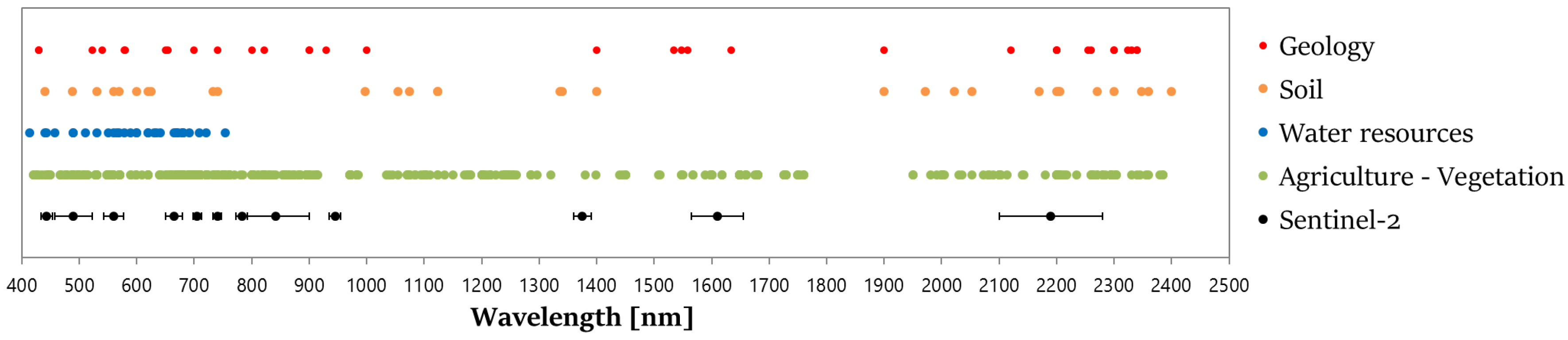
Figure 5.
Optimal (non-redundant) bands to retrieve the vegetation and agricultural crops biophysical parameters according to Thenkabail et al. [16] and Miglani et al. [25] compared to S2 center wavelengths (black dots). The bandwidth of the S2 bands are indicated by the bars.
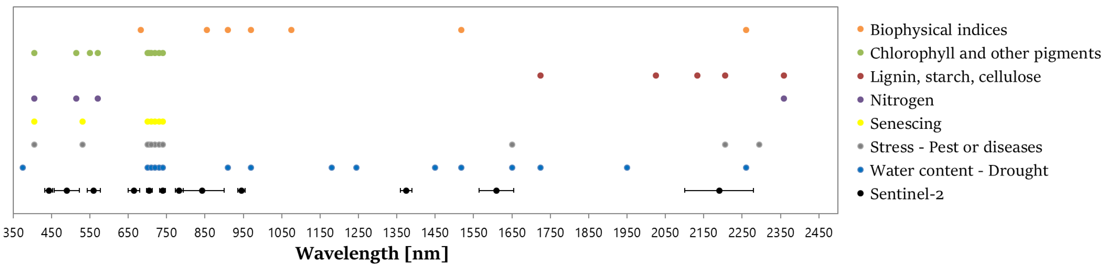
Table 1.
Comparison of the S2 sensors specifications with the Hyperion, TianGong-1 (TG-1), PRISMA and HISUI sensors’ characteristics [26,27,28,29,30].
| Instrument | MSI | Hyperion | TianGong-1 | PRISMA | HISUI |
|---|---|---|---|---|---|
| Platform name | Sentinel-2 | EO-1 | Shenzhou-8 | PRISMA | HISUI |
| Sensor type | Multispectral | Hyperspectral | Hyperspectral | Hyperspectral | Hyperspectral |
| Swath width (km) | 290 | 7.5 | 10 | 30 | 30 |
| Spectral range (nm) | 443–2190 | 357–2576 | 400–2500 | 400–2505 | 400–2500 |
| VNIR | 357–1000 | 400–1000 | 400–1010 | 400–970 | |
| SWIR | 900–2576 | 1000–2500 | 920–2500 | 900–2500 | |
| Spectral bands | 13 | 220 | 128 | 249 | 185 |
| Resolution | |||||
| Spatial (m) | 10–20–60 | 30 | 10 (VNIR) | 30 | 30 |
| 20 (SWIR) | |||||
| Temporal (day) | 5 | 16–30 | 14 to 7 | 2–60 | |
| Spectral (nm) | 15–180 | 10 | 10 (VNIR) | 10 | 10 (VNIR) |
| 23 (SWIR) | 12.5 (SWIR) | ||||
| SNR (30% albedo) | |||||
| VNIR | 89:1 to 168:1 | 144:1 to 161:1 | 200:1 | ≥450 at 620 nm | |
| 600:1 at 650 nm | |||||
| SWIR | 50:1 to 100:1 | 40:1 to 110:1 | 200:1 | ≥300:1 at 2100 nm | |
| 400:1 at 1550 nm | |||||
| 100:1 | |||||
| 200:1 at 2100 nm | |||||
| Objective | Earth observation | Earth observation | Scientific research and land imaging | Natural resources and atmosphere | Energy, vegetation monitoring |
| Country | Europe | USA | China | Italy | Japan |
| Organization | ESA | NASA | Chinese Academy of Science Physics | Agenzia Spaziale Italiana | Japanese Ministry of Economy, Trade, and Industry |
| Number of articles | 41 | 608 | 8 | 5 | 1 |
Table 2.
Comparison of the specifications of the S2 sensors with the EnMAP, SHALOM, HyspIRI and HypXIM sensors’ characteristics [9,15,26,31,32,33,34,35].
| Instrument | MSI | EnMAP HSI | SHALOM | HyspIRI | HypXIM |
|---|---|---|---|---|---|
| Platform name | Sentinel-2 | EnMAP | Improved Multi- | HyspIRI | HypXIM |
| Purpose Satellite-II | |||||
| Sensor type | Multispectral | Hyperspectral | Hyperspectral | Hyperspectral | Hyperspectral |
| Swath width (km) | 290 | 30 | 30 | 145–600 | 15 |
| Spectral range (nm) | 443–2190 | 420–2450 | 400–2500 | 380–2510 | 400–2500 |
| VNIR | 420–1000 | 400–1010 | 380–1400 | 400–1100 | |
| SWIR | 900–2450 | 920–2500 | 1400–2510 | 1100–2500 | |
| Spectral bands | 13 | 244 | 275 | 214 | 210 |
| Resolution | |||||
| Spatial (m) | 10–20–60 | 30 | 10 | 30 (60) | 8 |
| Temporal (day) | 5 | 27 (VZA ≥ 5) | 4 (VZA ≥ 30) | 5–16 | 3–5 |
| 4 (VZA ≥ 30) | |||||
| Spectral (nm) | 15–180 | 6.5 (VNIR) | 10 | 10 | 10 |
| 10 (SWIR) | |||||
| SNR (30% albedo) | |||||
| VNIR | 89:1 to 168:1 | 400:1 | 200:1 | 560:1 at 500 nm | ≥200:1 to 250:1 |
| >400:1 at 495 nm | 600:1 at 650 nm | ||||
| SWIR | 50:1 to 100:1 | 180:1 | 200:1 | 356 at 1500 nm | ≥100:1 |
| >180:1 at 2200 nm | 400:1 at 1550 nm | 236 at 2200 nm | |||
| 100:1 | |||||
| 200:1 at 2100 nm | |||||
| Objective | Earth observation | Earth observation | Land and ocean observation | Volcanic, vegetation, soil, exploration | Soil, urban, coastal, biodiversity |
| Country | Europe | Germany | Italy-Israël | USA | France |
| Organization | ESA | GFZ-DLR | ASI-ISA | JPL-NASA | CNES |
| Number of articles | 41 | 41 | 2 | 35 | 1 |
Table 3.
Article distribution classified according to the accomplishment of their respective objectives (i.e., (a) satisfactory, (b) moderate, (c) not satisfactory).
Table 3.
Article distribution classified according to the accomplishment of their respective objectives (i.e., (a) satisfactory, (b) moderate, (c) not satisfactory).
| Results | S2 | Hyperion | TG-1 | PRISMA | EnMAP | HISUI | SHALOM | HyspIRI | HypXIM |
|---|---|---|---|---|---|---|---|---|---|
| (a) | 77.8% | 57.7% | 50.0% | 50.0% | 63.0% | 100.0% | 100.0% | 40.6% | 100.0% |
| (b) | 22.2% | 30.8% | 50.0% | 50.0% | 29.6% | 0.0% | 0.0% | 46.9% | 0.0% |
| (c) | 0.0% | 11.5% | 0.0% | 0.0% | 7.4% | 0.0% | 0.0% | 12.5% | 0.0% |
| Studies | 27 | 78 | 2 | 6 | 27 | 1 | 1 | 32 | 1 |
Table 4.
Requirements of the main applications in terms of spatial, temporal and spectral resolutions mainly based on the HypXIM preliminary study of Briottet et al. [192] and our hyperspectral application literature. Each type of resolution is described as a high (+++), medium (++) and low (+) resolutions. High, medium and low spatial resolution respectively refer to <10 m, from 10–30 m and >30 m; and refers to ≤10 days, from 10–30 days and >30 days for temporal resolution.
| Main Applications Topics | Applications | Resolutions | |
|---|---|---|---|
| Spatial | Temporal | ||
| Vegetation and Agriculture | Monitoring/Status | +++ | +++ |
| Monitoring/Disease | +++ | +++ | |
| Classification | ++/+++ | +++ | |
| Geology and Soils | Mapping/Properties | ++/+++ | + |
| Exploration | +++ | + | |
| Land use | Classification/Changes | ++ | + |
| Urban | Classification/Changes | +++ | + |
| Water resources | Quality assessment | + | + |
| Bathymetry | + | + | |
| Classification of coastal ecosystems | + | + | |
| Component bloom | ++ | +++ | |
| Disaster | Prevention | ++ | +/+++ |
| Monitoring | ++/+++ | +++ | |
| Post-crisis | ++ | +/++ | |
© 2018 by the authors. Licensee MDPI, Basel, Switzerland. This article is an open access article distributed under the terms and conditions of the Creative Commons Attribution (CC BY) license (http://creativecommons.org/licenses/by/4.0/).
Share and Cite
MDPI and ACS Style
Transon, J.; D’Andrimont, R.; Maugnard, A.; Defourny, P. Survey of Hyperspectral Earth Observation Applications from Space in the Sentinel-2 Context. Remote Sens. 2018, 10, 157. https://doi.org/10.3390/rs10020157
AMA Style
Transon J, D’Andrimont R, Maugnard A, Defourny P. Survey of Hyperspectral Earth Observation Applications from Space in the Sentinel-2 Context. Remote Sensing. 2018; 10(2):157. https://doi.org/10.3390/rs10020157
Chicago/Turabian StyleTranson, Julie, Raphaël D’Andrimont, Alexandre Maugnard, and Pierre Defourny. 2018. "Survey of Hyperspectral Earth Observation Applications from Space in the Sentinel-2 Context" Remote Sensing 10, no. 2: 157. https://doi.org/10.3390/rs10020157
Note that from the first issue of 2016, this journal uses article numbers instead of page numbers. See further details here.