Improved Co-Registration of Sentinel-2 and Landsat-8 Imagery for Earth Surface Motion Measurements


1
École et Observatoire des Sciences de la Terre-EOST/CNRS UMS 830, University of Strasbourg, 67084 Strasbourg, France
2
Laboratoire des Sciences de L’ingénieur, de L’informatique et de L’imagerie, ICube/CNRS UMR 7357, University of Strasbourg, 67412 Illkirch, France
3
Institut de Physique du Globe de Strasbourg-IPGS/CNRS UMR 7516, University of Strasbourg, 67084 Strasbourg, France
*
Author to whom correspondence should be addressed.
Remote Sens. 2018, 10(2), 160; https://doi.org/10.3390/rs10020160
Submission received: 4 December 2017
/
Revised: 2 January 2018
/
Accepted: 9 January 2018
/
Published: 23 January 2018
(This article belongs to the Special Issue Analysis of Multi-temporal Remote Sensing Images)
Abstract
:The constellation of Landsat-8 and Sentinel-2 optical satellites offers opportunities for a wide range of Earth Observation (EO) applications and scientific studies in Earth sciences mainly related to geohazards. The multi-temporal co-registration accuracy of images provided by both missions is, however, currently not fully satisfactory for change detection, time-series analysis and in particular Earth surface motion measurements. The objective of this work is the development, implementation and test of an automatic processing chain for correcting co-registration artefacts targeting accurate alignment of Sentinel-2 and Landsat-8 imagery for time series analysis. The method relies on dense sub-pixel offset measurements and robust statistics to correct for systematic offsets and striping artefacts. Experimental evaluation at sites with diverse environmental settings is conducted to evaluate the efficiency of the processing chain in comparison with previously proposed routines. The experimental evaluation suggests lower residual offsets than existing methods ranging between = 2.30 and 2.91 m remaining stable for longer time series. A first case study demonstrates the utility of the processor for the monitoring of continuously active landslides. A second case study demonstrates the use of the processor for measuring co-seismic surface displacements indicating an accuracy of 1/5 th of a pixel after corrections and 1/10th of a pixel after calibration with ground measurements. The implemented processing chain is available as an open source tool to support a better exploitation of the growing archives of Sentinel-2 and Landsat-8.
1. Introduction
The constellation of Landsat-8 [1] and Sentinel-2 optical satellites [2] have a great potential to be used synergetically for a variety of Earth Observation (EO) applications due to their similar spectral and spatial properties and free and open data access. This comprises the monitoring of land cover changes, agricultural crops, biophysical parameters, continental waters, urban areas geomorphological processes (glaciers, landslides) to name a few. The accurate multitemporal co-registration of optical image time series is an indispensable pre-requisite for many analysis techniques including change detection [3,4], land cover classification [5] and Earth surface motion quantification [6].
At the time of initiating this work, the multi-temporal co-registration accuracies of Sentinel-2 products from the same orbit and ingested after 15 June 2016 is 12 m ([email protected]%). Products before that date were affected by a yaw bias correction anomaly leading to accuracies of up to 18.3 m for products processed before 15 June 2016 including across-track offsets with a stripe-like pattern in the along-track direction [7,8]. These figures are not yet compliant with the mission specifications of 3 m, which are expected to be met only after activation of the nearly completed (end 2017) global reference image [8,9].
As already noted in [10], coregistration residuals are also related to errors in the topographic model used for orthorectification of the Sentinel-2 L1C products and are hence spatially inhomogeneous. The PlanetDEM90 [11] is used for the orthorectification of L1C products and comprises an elevation uncertainties of 16 m (2). These elevation uncertainties affect the geolocation accuracy and, at the border of the swaths where the off-nadir view angle reaches 10.5, translate into offsets of 2.95 m. As a consequence the multi-temporal co-registration accuracy of 12 m ([email protected]%) does not apply for products acquired from neighbouring overlapping swaths where the PlanetDEM90 uncertainty and the maximum convergence angle of 21 translate into additional offsets of up to 5.9 m [8,10].
The geolocation accuracy of Landsat-8 L1T products is currently estimated at 35 m ([email protected]%) due to issues in the reference Global Land Survey. The specified geolocation accuracy of Sentinel-2 is 12.5 m ([email protected]%). This leads to an estimated co-registration error of 38 m ([email protected]%) between Sentinel-2 L1C and Landsat-8 L1T products [12]. Considerable greater offsets among the two products may arise locally due to a combination of different viewing geometries and digital elevation models (DEM) used for orthorectification [10].
In summary, horizontal offsets of approximately one 10 m pixel among Sentinel-2 L1C products of the same orbit, of up to four 10 m pixel among Sentinel-2 L1C and Landsat-8 L1T products must be expected. While both ESA and NASA are working to solve these issues, it is estimated that the reprocessing of Landsat-8 data could take until late 2018, whereas a reprocessing schedule for Sentinel-2 data has not been established yet [8,12]. Given that even sub-pixel offsets have detrimental impact on the accuracy of time-series analyses [3,13,14,15] and in particular surface motion measurements [6,10,16,17], improved geometric pre-processing constitutes an essential step to exploit image time-series. While this applies in general for the analysis of images acquired by different satellite and aerial platforms this study focuses in particular on Sentinel-2 and Landsat-8 which are both freely and globally available with standardized formats and similar spatial and spectral characteristics.
Image co-registration is a classical and well-studied problem. Proposed methodologies differ in particular regarding the employed matching algorithms (e.g., area-based vs. feature-based matching) and the mapping function used to estimate the transformation from one image to another. While comprehensive surveys of proposed algorithms can be found in [18,19,20,21] we focus in the following on recently proposed approaches that target the co-registration of multi-sensor remote sensing images and in particular Sentinel-2 and Landsat-8 imagery.
A complex routine for the co-registration of multi-sensor optical images including Landsat-7, ASTER, SPOT-1 and 5 and RapidEye imagery was recently proposed in [22]. The routine relies on Landsat-7 as reference imagery and uses normalized-cross correlation to sample at most 100 tie points for the estimation of a simple translational transform. A global RMSE after co-registration of 17 m is reported by the authors. The authors of [23] presented the open-source tool AROSICS targeting a robust and fast co-registration of multi-sensor satellite data. The routine relies on a sub-pixel phase correlation algorithm [24] to extract thousands of tie points on regular grids, filtering of outlier matches using Mean Structural Similarity Index [25] and a Random Sampling Consensus (RANSAC, [26]) to estimate an affine image transformation. The authors present a limited set of experiments indicating an RMSE of 4.45 m for the co-registration of Landsat-8 to Sentinel-2, 4.5 m for the co-registration of Landsat-8 to RapidEye-5, and 0.9 m for the co-registration of TerraSAR-X (StripMap mode) images. Similar figures were also reported by [27] for the co-registration of Landsat-8 to Sentinel-2 imagery targeting the harmonization of both datasets at 10 m in the tiling scheme defined by the Landsat Data. The routine comprises feature point detection and least-square matching which are used to parametrize three transformation functions including simple translation, an affine transformation and a second order polynomial. An experimental evaluation with three image pairs suggests the suitability of an affine transformation to reach a residual RMSE of approximately 3 m. The method does, however, not account for along-track striping artefacts and slight offsets among overlapping seams of Landsat-8 images from different paths and rows. More recently [28] proposed and extensively tested a method that relies on a phase-correlation algorithm [29] to extract thousands of tie-points on a regular grid, RANSAC for filtering outliers and different transformation functions including translation, affine transformation, radial basis function, thin plate splines and Random Forest (RF) regression. They report co-registration residuals based on tie points which were not used for the model estimation but pre-filtered using RANSAC. The performance of different transformation functions was similar with the RF regression performing slightly better. The reported RMSEs are in the range of only 1 m for both the co-registration of Landsat-8 to Sentinel-2 and Sentinel-2 to Sentinel-2.
All these approaches target in particular the fast co-registration of Sentinel-2 and Landsat-8 imagery and take advantage of a limited set of automatically detected tie points ranging from a few 100 to a few 1000 points. While this reduces the computation time it does not allow generating and correcting dense offset measurements required for Earth surface motion quantification. Furthermore, along-track striping artefacts are only addressed implicitly by using non-linear models such as RF regression, which however will also model and correct for ground motion. To address those issues, we propose the coregis processor which has been designed to address both highly accurate co-registration of Sentinel-2 and Landsat-8 data and surface motion measurements. The contribution of the study is fourfold:
- Develop a processor that is suitable for both the co-registration of Sentinel-2 and Landsat-8 imagery and the correction of co-registration residuals in dense surface motion measurements;
- Provide a comprehensive experimental evaluation of the processor in comparison with previous studies;
- Present and discuss two operational use cases of surface motion measurements for which coregis is usefull;
- Provide an open source toolbox that implements coregis.
2. Methods and Data
2.1. Image Matching
For the computation of dense surface motion maps, coregis builds on the open-source stereo-photogrammetric library MicMac [30] and in particular on the image-correlation algorithm detailed in [31]. The algorithm has several free parameters including the window size , the correlation threshold , the regularization parameter and the sub-pixel precisions , which in accordance to previous study [17] were set to , , and . Considering the estimated co-registration error of 38 m, the search range was set to 4 pixels (Sentinel-2, 10 m) or 40 m. For the Sentinel-2/Sentinel-2 case, the red band is used for matching since it is also used as the reference for band-to-band co-registration [8]. For the Landsat-8/Sentinel-2 case, a synthetic panchromatic band is generated from the three Sentinel-2 bands in the visible spectra and the Landsat-8 panchromatic band is reprojected to the Sentinel-2 tile layout at 10 m resolution before matching. The reprojection of the Landsat-8 panchromatic band is realized using bicubic resampling.
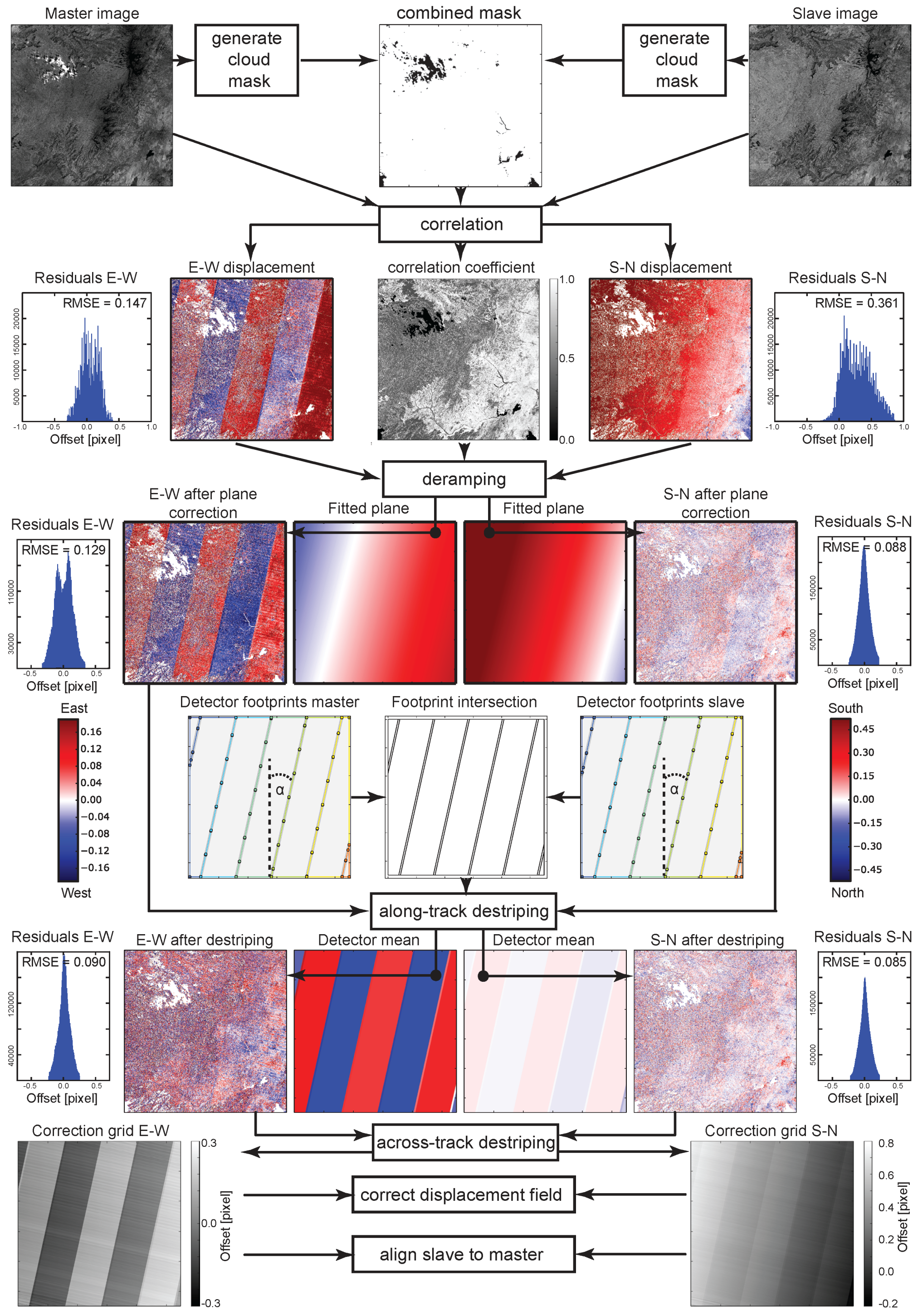
To reduce the computational load and the likelihood of erroneous matches due to clouds, snow cover or surface waters, the F-mask algorithm [32] is used to generate binary masks for each of the two input images. All pixels detected as clouds, snow or water are marked as 0. The combined mask (Figure 1 comprises the union of all pixels, which are marked as 0 and are hence ignored during the matching. The matching yields three output grids (E-W), (N-S) and (correlation coefficient) holding respectively , and for the ith pixel of the slave image relative to the master image.
2.2. De-Ramping
The obtained displacement fields typically comprise systematic offsets resulting mainly from translation and rotation among the input images. Considering an affine transformation the systematic offsets can be modelled with two planes denoted in Equations (1) and (2).
where and are the modelled offsets, and are the spatial coordinates of the ith pixel in the reference image and and are the unknown parameters of a plane. The unknowns are estimated using an iteratively reweighted least square (IRLS) with a bisquare loss function [33] minimizing the residuals between the measured and modelled offsets. Compared to other approaches, IRLS has the advantage of providing robust estimates with up to 50% outlier-contaminated samples. The modelled systematic offsets can be subsequently removed from the initial measurements (Equations (3) and (4)).
where and are the grids holding the offsets of the estimated plane ( and ) and and denote the grids holding the plane-corrected offsets.
2.3. De-Striping
The staggered sensor arrays of pushbroom satellites such as Sentinel-2 and Landsat-8 can lead to small systematic image offsets which manifest as along-track striping artefacts which are particularly visible in the component but can also be observed in the component (Figure 1). For Sentinel-2, this concerns in particular early acquisitions processed before yaw bias correction is applied in the processing baseline 2.04 [8]. For Landsat-8, a similar yaw bias correction is applied since October 2013 [34] including reprocessing of earlier scenes. Stripe-like artefacts can still be encountered in areas which are imaged with different detector elements in the master and slave image, respectively.
To correct these artefacts, the plane-corrected offsets are passed forward to a destriping routine. For the Sentinel-2/Sentinel-2 case both images are provided with metadata detailing the position of the detector footprints on the ground. The polygons delineating the detector footprints are intersected and the mean displacement and for each of the resulting polygons (along-track destriping Figure 1) is computed considering all pixels within the respective polygons. Given that Landsat-8 products are not provided with metadata on the detector footprints, the case of Landsat-8/Sentinel-2 is handled differently. The displacement field is rotated according to the ground track azimuth angle which is derived from the metadata of the master image, and and are computed for each image column. The image holding the column means is subsequently rotated back to the original geometry. An additional step for across-track destriping using the row means is also implemented in coregis but is not used in the presented experiments since analyses did not indicate a statistically significant reduction of the co-registration residuals.
The final correction grids (Figure 1) and are computed as the sum of all correction steps (Equations (5) and (6)). They serve for both purposes: (1) the correction of the initially obtained displacement fields to obtain and (Equations (5) and (6)), and (2) the resampling of the slave image into the geometry of the master using bicubic resampling.
2.4. Experimental Setup and Accuracy Assessment
A total 178 of Sentinel-2 and Landsat-8 images have been processed to assess the coregis processor in terms of co-registration accuracy and regarding its ability to provide the necessary corrections for displacement measurements. To enable comparison with previous studies, we rely partially on the datasets used in [27,28] where all images are co-registered to one master image (Supplementary Material Table S1/S2). This includes test sites in Argentina, Ukraine, USA and South Africa.
A further set of experiments is dedicated to the impact of increasing time lags between the master and slave images on the co-registration accuracy. To this end a dataset of 38 Sentinel-2 images acquired between 5 May 2016 and 21 August 2017 at a test site in the French Alps (tile 31TGK) is used (Supplementary Material Table S3).
Finally, the ability to correct co-registration artefacts for motion measurements is evaluated for two test cases comprising the monitoring of the Harmalière landslide/France (tile 31TGK, Supplementary Material Table S4) and the quantification of co-seismic slip resulting from the Kaikoura earthquake/New Zealand on November 14 2016 (tile 59GQP, Supplementary Material Table S5). The co-registration residuals are generally evaluated by the considering the residual offsets of all pixel (, ) with and n being the total number of pixels (Equation (7)).
To enable comparison with the work presented in [27] at the South African test sites we also compute the mean absolute error (MAE, Equation (8)).
As noted in [27,28], the offset measurements typically comprise gross matching errors which are not representative for co-registration accuracy and impact in particular the RMSE. To reduce the impact of such outliers, [27] used a threshold of approximately three times the RMSE of the matching residuals. In [28], the homologous points were filtered before the accuracy assessment using RANdom Sampling Consensus (RANSAC) with 99% confidence threshold and 100 iterations. This strategy, however, does not take into account the statistical distribution of the offset residuals (typically Gaussian) and removes data points rather aggressively (Supplementary Material, Figure S1). To avoid an underestimation of the co-registration errors, we used a strategy similar to [27] by fitting the and with a Gaussian distribution using a maximum likelihood estimator and removing all values outside the 99% confidence interval of the distribution. While this hinders a direct comparison with the results presented in [28], it yields higher and more realistic error estimates and allows a comparison with the results presented in [27].
3. Results and Discussion
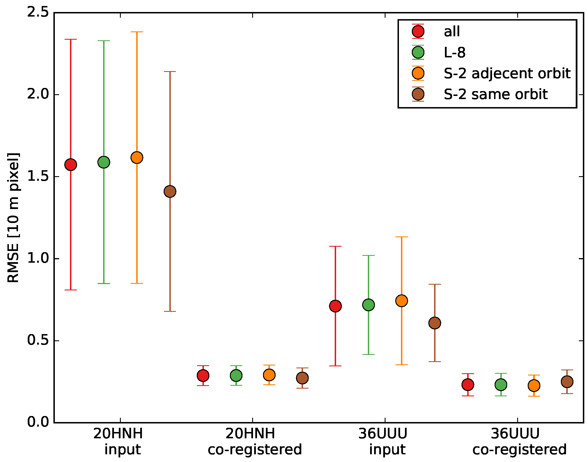
The results obtained for the five study cases suggested in [28] are displayed in Figure 2 and Figure 3. The co-registration errors before the correction vary considerably from site to site and according to the combination of input images; in particular for the tile 20HNH the average amounts to 16.17 7.67 m and 15.98 7.40 m for adjacent Sentinel-2 orbits and Sentinel-2 to Landsat-8 co-registration, respectively. The latter corresponds to a CE95 of 26.42 m which is somewhat lower than the 38 m assumed by the authors [12] which also noted that their estimate may be rather pessimistic since the Landsat-8 reference framework may be more accurate than specified.
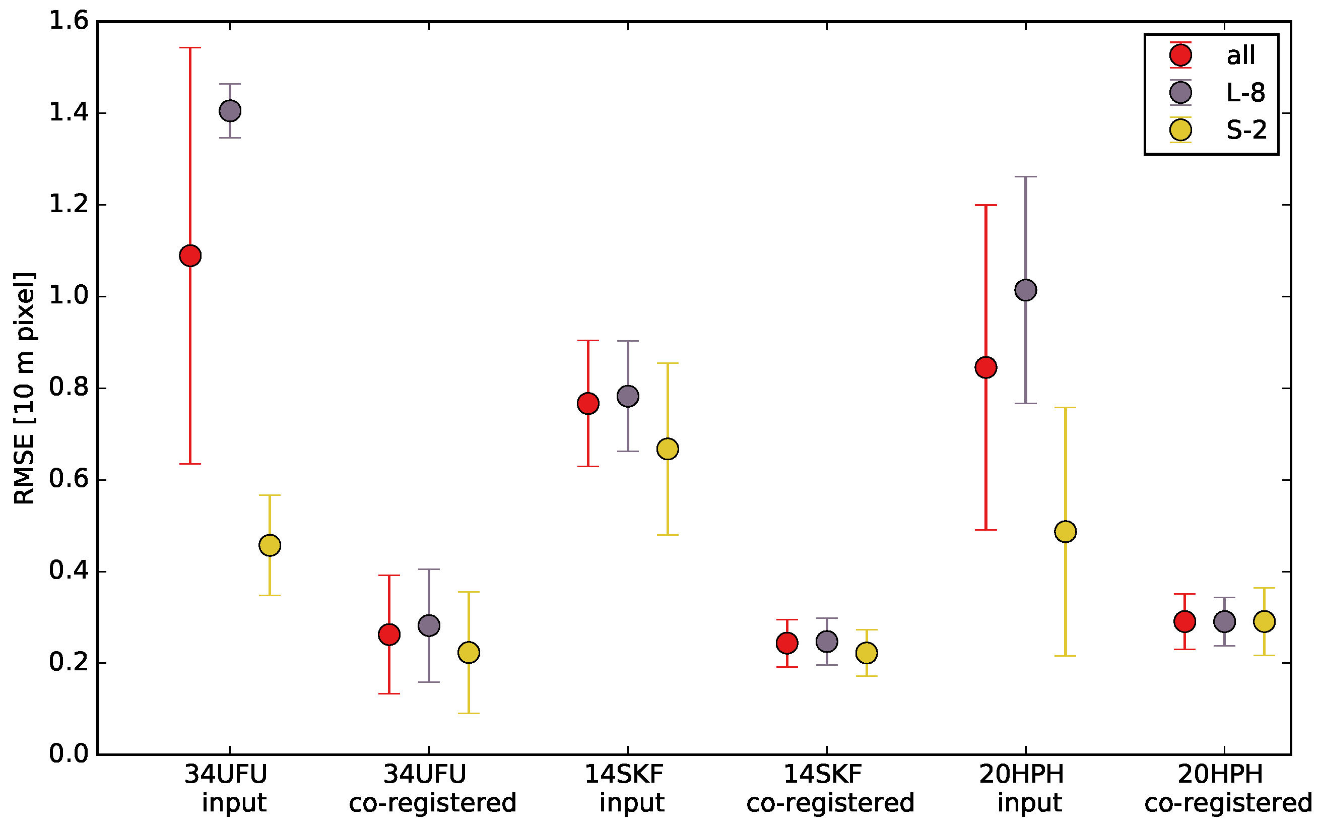
The initial among Sentinel-2 images acquired from the same orbit is generally lower ranging from 4.57 1.10 m for the tile 34UFU to 14.10 7.31 m for the tile 20HNH. For the sites displayed in Figure 3 the initial co-registration among Sentinel-2 and Landsat-8 is generally worth than for the Sentinel-2 to Sentinel-2 case with up to 14.54 0.06 for the tile 34UFU, whereas the same is not true for the two test site displayed in Figure 2. Considering that most Sentinel-2 scenes in these datasets were processed before the yaw bias correction, the initial co-registration errors are consistent with the expected errors (see Section 1).
Despite the great variability of the errors before corrections, the after the co-registration generally decreases below 4.78 m (maximum at the 20HPH test site) with mean of 2.87 0.61 m, 2.32 0.67 m, 2.62 1.29 m, 2.44 0.05 m, and 2.91 0.06 m for the tiles 20HNH, 36UUU, 34UFU, 14SKF, and 20HPH, respectively. The results are equally good for all cases (Sentinel-2 to Sentinel-2 same and adjacent orbits, Landsat-8 to Sentinel-2) suggesting that the coregis processor enables robust and accurate co-registration of Sentinel-2 and Landsat-8 for a wide range of environments.
3.1. Comparison with Previously Proposed Methods
For comparison with the previously proposed methods, coregis was applied to the Sentinel-2 tiles and Landsat-8 scenes suggested in [27]. As shown in Figure 4 the can be reduced to a range between 0.09 0.06 m and 1.13 0.09 m compared to between 2.10 1.70 m and 2.60 1.80 achieved with a 2nd order polynomial transformation used in [27]. We attribute these improvements to several methodological differences.
First, individual Sentinel-2 tiles are used as master and Landsat-8 scenes are co-registered individually avoiding the fusion of multiple Landsat-8 paths and rows before the co-registration. This is in particular important since we observed slight offsets among the images from neighbouring Landsat-8 rows which will lead to inconsistent reference images if both rows are merged beforehand. Second, coregis relies on the Landsat-8 panchromatic band which provides higher spatial resolution (15 m) than the near-infrared (30 m). Third, the destriping step explicitly addresses along-track stripes which are particularly pronounced for the South Africa test case. Fourth, the dense offset measurements computed with coregis provide, while being computationally expensive (see also Section 3.4), a complete sampling of the statistical distribution of the offsets used to estimate the image transformation.
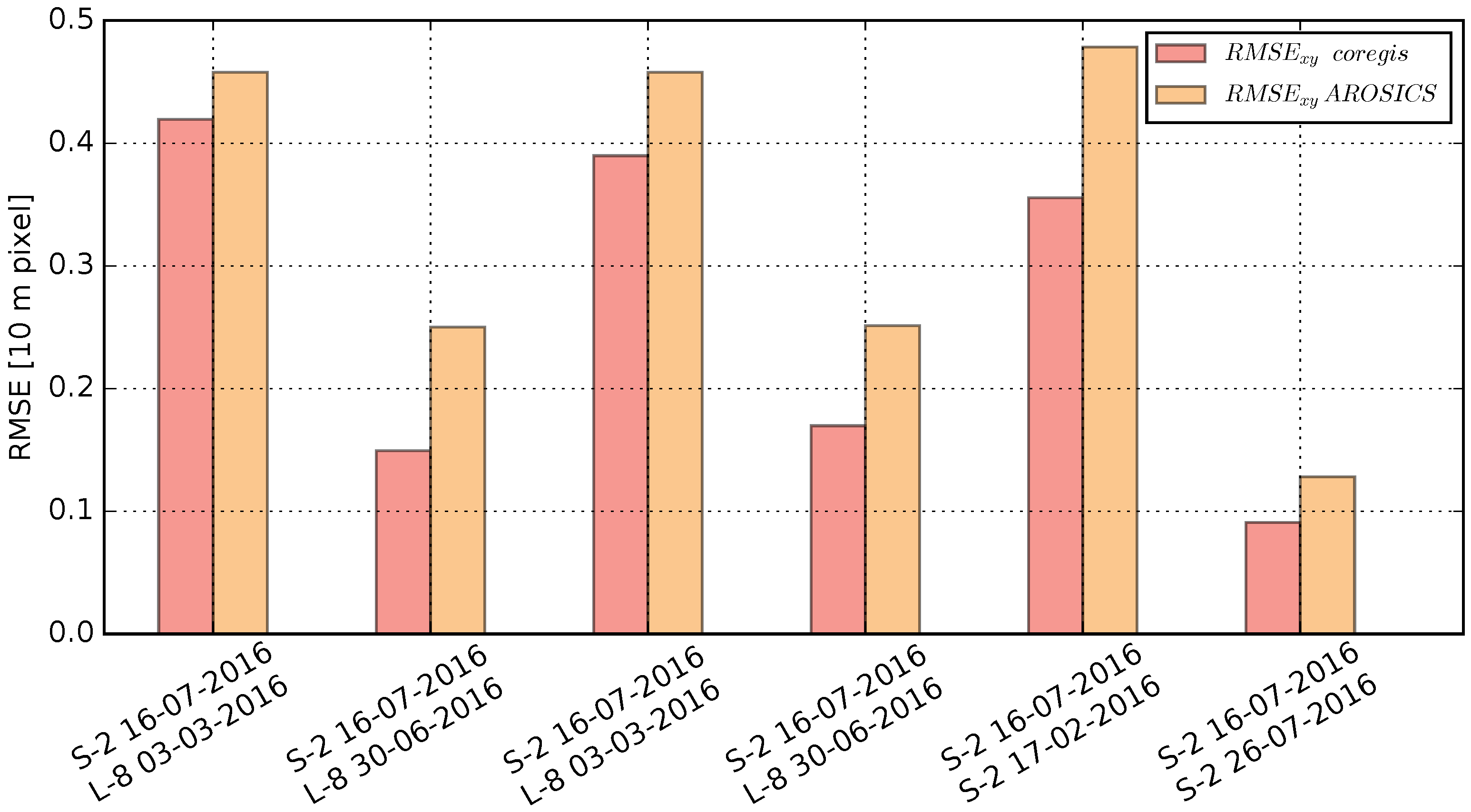
A second comparison with the AROSICS package [23] was performed using the images for the tile 34UFU. AROSICS was used with the recommended default parameters and sub-pixel image correlation was performed on the co-registered images to assess residual offsets. The are compared in Figure 5 showing a mean of 2.7 1.3 m with coregis compared to 3.4 1.3 m with AROSICS. The results suggest a slight but consistently higher accuracy of the coregis processor which can probably be attributed to denser offset measurements and the explicit handling of striping artefacts. It is also interesting to observe that the accuracies of both methods are strongly correlated among different tiles indicating that the image characteristics (e.g., seasonal changes, cloud cover) similarly affect the accuracy of both methods.
3.2. Time-Series Stability
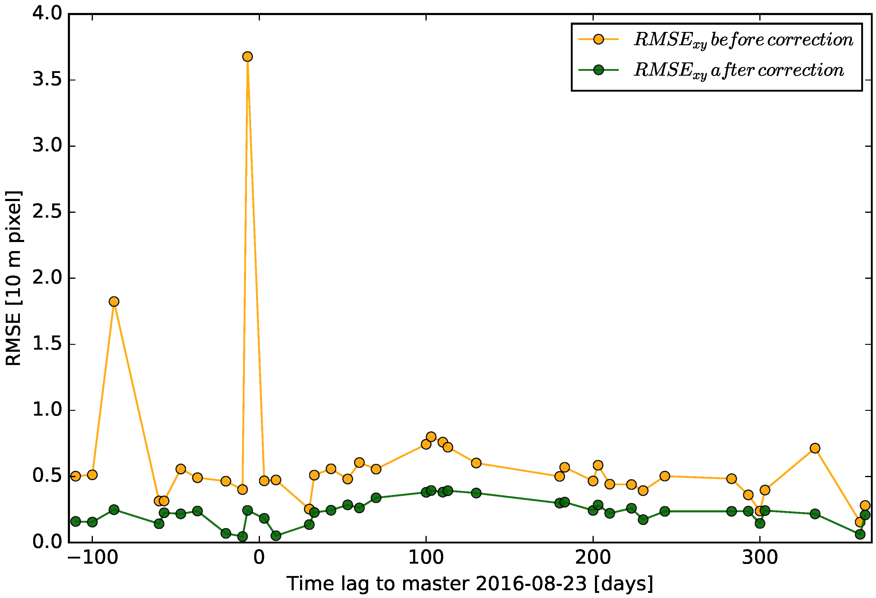
An important aspect for the analysis of image time-series is the temporal stability of the co-registration since surface changes accumulate over time and may deteriorate the co-registration accuracy relative to the defined master. As illustrated in Figure 6 the after the correction does not change significantly with the time lag to the defined master image indicating that the method can be used to co-register large image stacks spanning at least two years. For challenging sites such as mountainous areas or areas with important cloud and snow covers, the is 2.30 0.10 m and generally remains below 4 m. A slight increase can be observed for slave images recorded during December (time lag 100 to 130 days) which can probably be attributed to an increase in cloud and snow cover during the winter season. Of the two outliers with of 18.2 m and 36.8 m before correction only the first was marked for geometric problems in the metadata of the distributed Sentinel-2 L1C product.
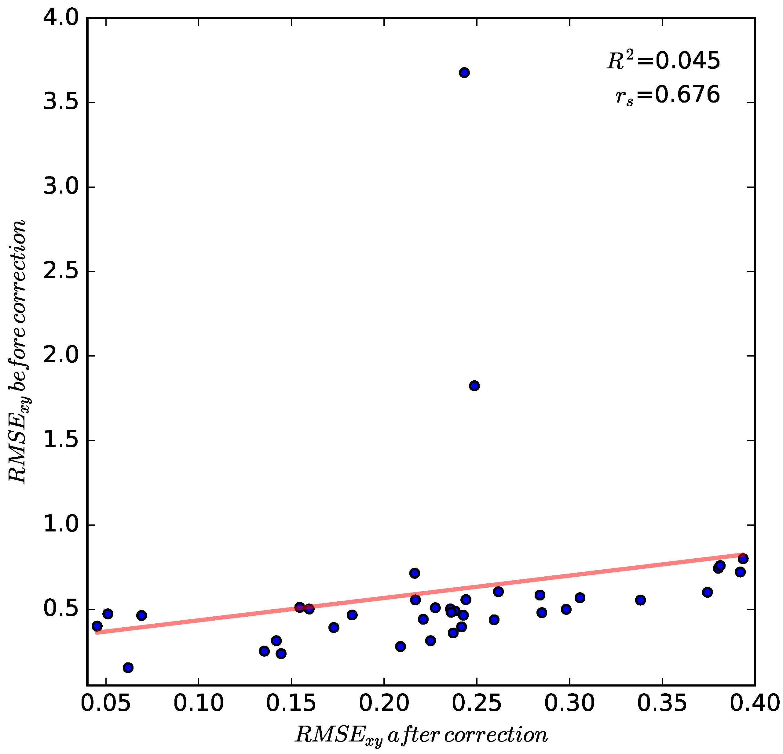
Interestingly, there is also a clear relationship between the magnitude of the residuals before and after the corrections. As shown in Figure 7 the relationship is not linear (low Pearson’s due to outliers) but monotonic (high Spearman rank correlation ). This indicates that Sentinel-2 L1C products with lower initial residuals also tend to display lower residuals after co-registration. This is likely due to the impact of orthorectification artefacts which cannot be corrected with the coregis processor.
3.3. Surface Motion Measurements
The coregis processor is conceived to provide corrections for both image co-registration and Earth surface displacement quantification. To evaluate the accuracy of the processor for motion measurements, two case studies related to the displacement analysis of the Harmalière landslide (Isère, French Alps) during an acceleration period and the measurements of the co-seismic slip associated to the Kaikoura earthquake (New Zealand, 2016) are presented.
3.3.1. Surface Displacement Analysis of a Large Landslide
The Harmalière landslide, located 30 km South of Grenoble in the Trièves region (French Alps) develops in clay-rich glaciolacustrine sediments. It has been particularly active between 1981 and 2003 with an average surface displacement of 10 m year [35,36]. The most active part of the landslide currently measures approximately 1.6 km from the head scarp to the toe with an average slope of around 10. Observations at the neighbouring Avignonet landslide suggest that surface displacement is accommodated at several slip surfaces at depths up to 40 m. Further details on the topographic and geologic controls of the landslide surface kinematics can be found in [37]. The landslide underwent another abrupt acceleration starting 27 June 2016.
To document this period of acceleration, a time-series of 31 Sentinel-2 images and 1 Landsat-8 image spanning the period 5 May 2016 to 21 August 2017 (Supplementary material, Table S4) were processed. To assure that the landslide motion is fully captured was increased to 15 pixels (i.e., 150 m). Each image was correlated with the three previous acquisitions to construct a redundant network of displacement measurements from which the final time-series is constructed by eliminating pairs with higher values while retaining a seamless time-series covering the full study period. In addition, for each pair, the correlation was performed once with the master-slave in temporal order and once in the inverted order. For each pair these measurements are averaged providing further robustness against noise and gross outliers. From the 90 computed displacement maps a total of 22 maps were selected by removing scenes with a co-registration > 3 m and avoiding pairs of neighbouring orbits while retaining sufficient pairs to construct a time-series which provides full coverage of the surface motion.
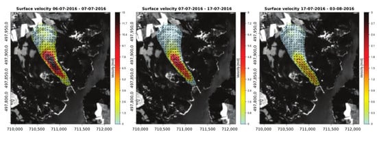
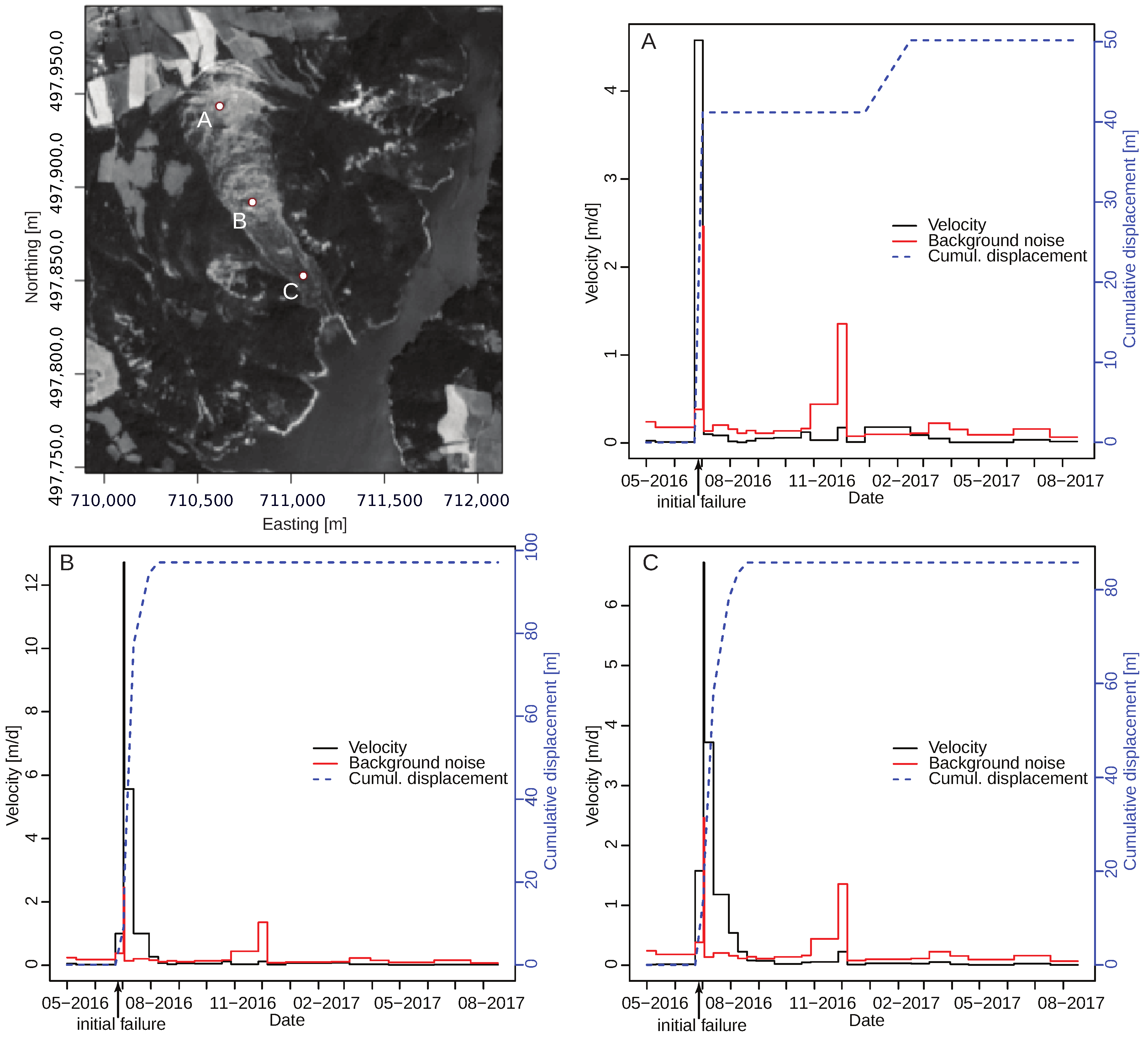
The resulting surface velocity time-series are shown exemplaryly for three points close to the head scarp (A), in the transport zone (B) and close to the toe of the landslide (C) in Figure 8. The background noise after the corrections resulting from orthorectification errors is evaluated considering the 95% quantile of the velocities measured on stable terrain surrounding the landslide.
The maximum velocities exceeding the level of the background noise were measured between 6 July 2016 (Landsat-8) and 7 July 2016 (Sentinel-2) amounting to 13.3 m day (meter per day) demonstrating the value of the combined use of Sentinel-2 and Landsat-8 during periods of fast surface motion. The maximum displacement rate was likely achieved shortly after the initial failure of 27 June 2016 but is not fully captured by the previous image pair (27 June 2016 to 6 July 2016) due to decorrelation induced by strong surface changes. Velocities measured before the initial failure are close to zero and clearly below the noise level indicating that no precursory movement could be detected for this event.
After the initial failure the upper part of landslide decelerated relatively quickly while motion at the toe (Figure 8C) remained above the noise level until 22 September 2016 at 0.32 m day. A further reactivation with velocities of up to 0.40 m day at the head scarp is captured for the period 31 December 2016 till 19 February 2017. The correctness of the detection is supported by field observation of a strong reactivation at the head scarp on 29 January 2017.
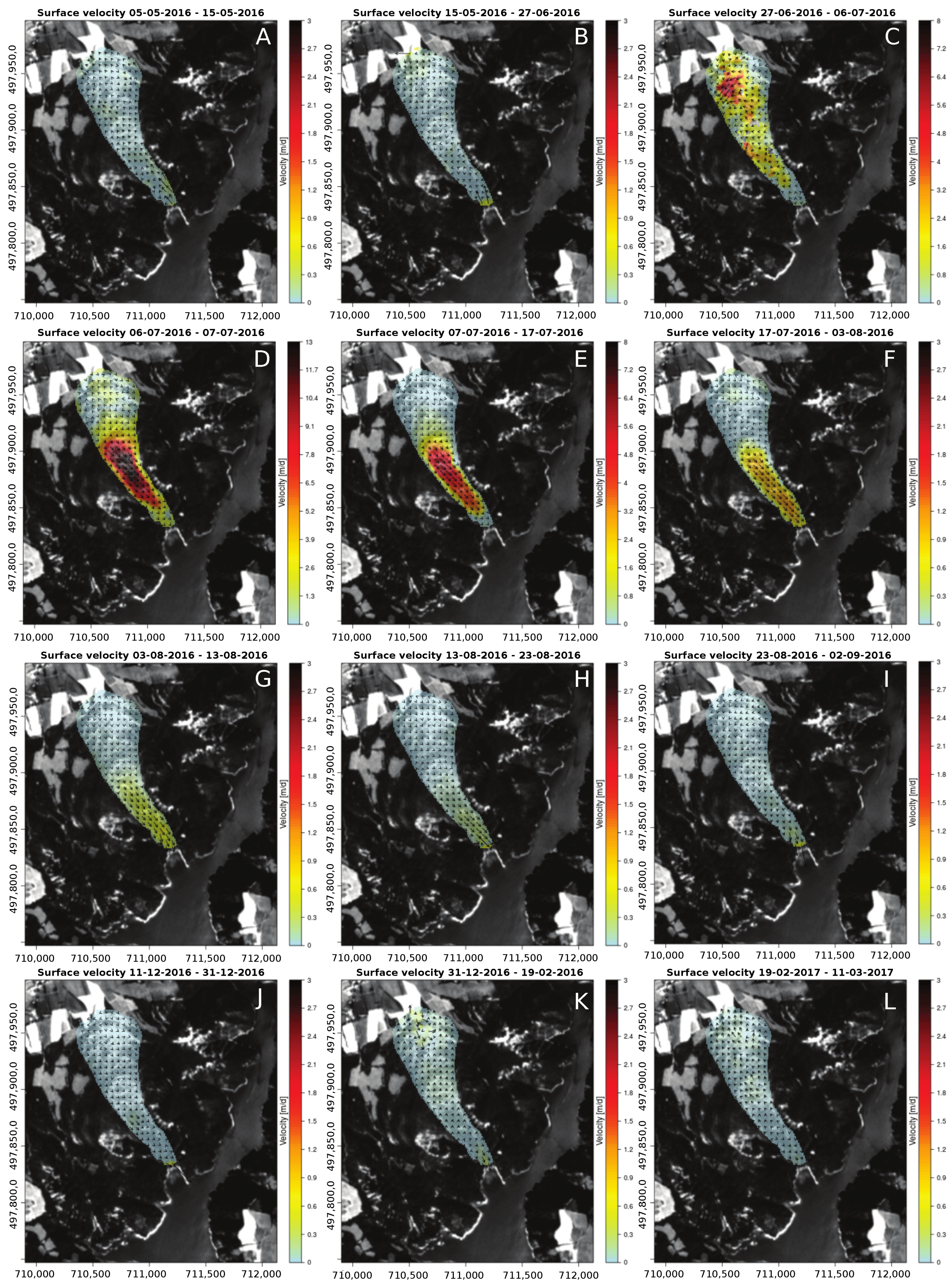
The displacement maps covering the initial activation in 2016 and the reactivation in early 2017 are presented in Figure 9. The evolution of the surface motion pattern shows an acceleration that initiated with retrogressive failures at the head scarp, whereas the toe remained initially stable. Transverse scarps are visible in the images after the reactivation at the upper and central part of the landslide (Figure 8, point A and B). The flow-like motion pattern suggest that strain is mainly accommodated by remoulding of the resulting blocks and deformation of fine grained matrix rather than by the movement of individual coherent blocks. After the initial failure, the largest measured displacements are observed at a secondary scarp at the centre of the landslide Figure 8 and Figure 9, point B). Below this section, the slopes are generally below 10, transverse scarps are absent and the landslide evolves into a mudflow. The propagation of the movement from the head scarp to the toe suggests that the toe constitutes a stabilizing element and that motion at the toe is induced through increased loading with material arriving from upslope. The observed velocities decrease rather abruptly towards the lateral limits of the landslide possibly indicating a stabilizing impact of lateral shear.
3.3.2. Surface Displacement Analysis of Co-Seismic Slips
Kaikoura is located at the north-eastern South Island of New Zealand. The area was struck by a major M 7.8 earthquake on 14 November 2016 (NZDT). Several studies have already documented the rupture mechanism and co-seismic slip with satellite imagery including the use of image correlation with Landsat-8 [38] and cubesat imagery [39], as well as the inversion of 3D displacements from offsets tracking with ascending and descending Sentinel-1 images [40]. The event provides a use case to evaluate the coregis processor capability to quantify surface displacement induced by strong earthquakes. The earliest post-earthquake Landsat-8 and Sentinel-2 images recorded after the event (29 November 2016 for Landsat-8, 22 November 2016 for Sentinel-2) provide only limited coverage due to cloud cover and path geometry, respectively.
To obtain full coverage and obtain redundant measurements that allow a better quantification of the measurement uncertainties, we used 4 Sentinel-2 pre-earthquake and 5 Sentinel-2 post-earthquake images (Supplementary Material Table S5). Given that the post-seismic slip was limited to a maximum of 40 cm [41], we assume that the correlation-based measurements are by far dominated by the co-seismic slip (see also, [40]). We compute a total of 40 displacement maps considering all possible pre-post-earthquake images in forward temporal master-slave order and backward temporal order resulting in two displacement maps per image pairs. The parameters for the sub-pixel image correlation are set to , , , and . After deramping and along-track destriping corrections, the two forward-backward displacement maps for each image pair are averaged; this procedure results in a slight reduction of noise due to mismatches. The final displacement maps are computed by independently stacking the two horizontal components of the 20 displacement maps; a sliding window of the median of all measurements (with a sliding window size of 11 pixel (i.e., 110 m)) is used.
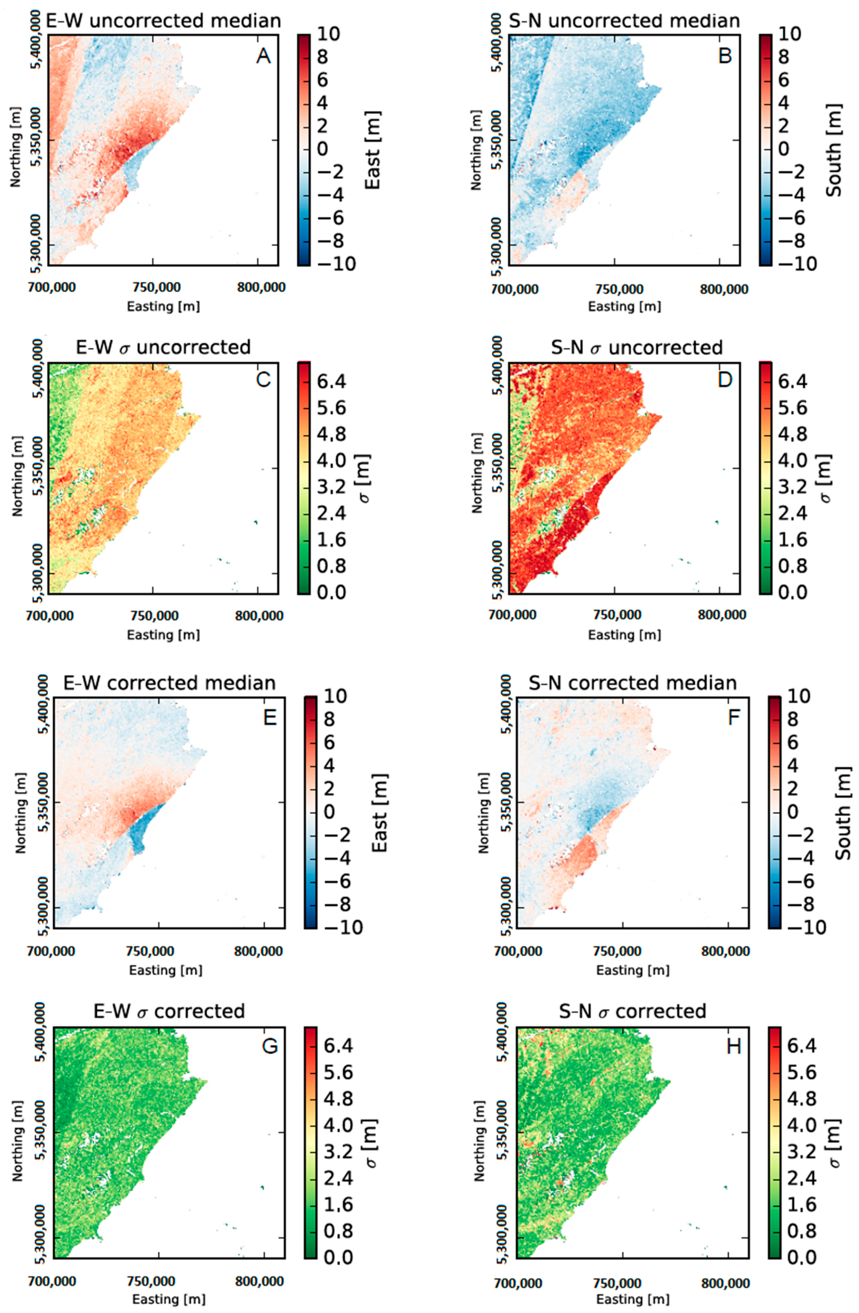
The effect of the corrections is evaluated by comparing the resulting displacement maps and the variance for each pixel among the 20 independent measurements before and after corrections. As shown in Figure 10 the median displacements without corrections are strongly contaminated by offsets due to the orbital errors and the staggered sensor array. This results in average standard deviations of 4.03 1.13 m in the EW-component and 5.23 1.41 m in the NS-component before the corrections.
A visual assessment of the median components after the correction suggests an efficient removal of systematic offsets. The maximum horizontal along-fault slip of up to 10.6 m is observed on the north-eastern segment of the Kekerengu fault (Supplementary material, Figure S2) which is well in line with field observations of 9–11 m [42]. Similarly the fault slip estimated on the northern part of the Papatea fault agrees well with more than 2 m slip in the field, whereas our measurements suggest a horizontal fault slip of not more than 1.8 m on the southern end of this fault, which is clearly lower than 5–6 m estimated in the field.
The average standard deviations () after the corrections (Figure 10) suggest measurements uncertainty of 1.61 0.07 m in the EW-component and 1.67 1.00 m in the NS-component. A comparison with 29 point-wise GPS measurements provided in [40] suggests RMSEs with a similar magnitudes being 1.77 m in the EW-component and 1.47 m in the NS-component. This comparison also shows mean errors of −1.66 m in the EW-component and −0.92 m in the NS-component indicating a deficits of eastward and northward displacements in our measurements. This is likely due to the lack of stable terrain within the scene extent leading to a bias in the statistical plane fitting (see also Section 3.4) towards east and north offsets dominant in north-east of the scene. The problem can be alleviated by using a simple linear regression as a calibration method to scale the image-based measurements against in situ measurements. To this end we run a 10-fold cross-validation which suggests that a calibration against ground measurements further reduces the RMSE to 0.55 m in the EW-component and 1.13 m in the NS-component.
3.4. Current Limitations and Further Directions
The experimental results for the coregistration performance of coregis suggest an which is generally between 2 and 3 m and hardly exceeds 4 m. Experiments indicate that the method is more accurate than previously proposed approaches [23,27] and provides stable results for long time series. Despite those positive characteristics of the processor it also comprises several limitations that users should take into account concerning in particular the elevated computational load, possible statistical bias and the lack of local corrections for orthorectification errors.
Sub-pixel image correlation is generally a computational expensive operation and the matching of two Sentinel-2 scenes (10,980 × 10,980 pixel) generally requires 30–40 min on a work station (e.g., 8 cores at 3 GHz each) depending on the degree of cloud cover and decorrelation within the scene. A significant reduction of the computing time can be achieved by reducing the resolution of the output grids and/or reducing the sub-pixel precision which should enable to adapt coregis also to applications for which processing speed is more important than accuracy. To reduce the computing time for this study all image pairs presented were computed on a dedicated HPC infrastructure. The coregis processor is available as a stand-alone service on the Geohazards Exploitation Platform (GEP) of the European Space Agency geohazards-tep.eo.esa.int. The underlying Python code is also publicly available at github.com/andrestumpf/coregis_public.
As shown in Section 3.3.2, the purely statistical approach of the correction can introduce biases when most of the scene is affected by ground motion. This is a general limitation of statistical correction methods (e.g., [6,23,27,28]) and biases will typically increase if the displacement fields are fitted with higher order functions. Prior knowledge of the spatial distribution might in some cases be useful to mask out areas with significant ground motion and, as demonstrated in Section 3.3.2, in situ measurements can be used for calibration. Further work on coregis will address this issue by enabling the mosaicking of multiple tiles to ensure that sufficient stable terrain supports the statistical corrections.
It should be recalled that currently all corrections are global and cannot address local orthorectification errors. This limits the measurement accuracy particular in mountainous terrain and remains the main source of background noise as presented in Section 3.3.1. For areas with locally homogeneous DEM errors and thus orthorectification errors, supplementary local statistical corrections could be used to address this issue. Furthermore, the residual displacements on stable terrain could also be used to weight individual measurements within the framework of time-series inversion strategies such as presented in [43,44]. Recent works also demonstrate that observations from different orbits can be used to quantify the unknown DEM errors and correct displacement measurements [45]. The applicability of this technique remains, however, limited to displacements in the along-track direction of the satellite.
Finally, image correlation of quasi-simultaneously acquired Sentinel-2 bands can also be used to detect fast moving (>4.7 m s) and high-altitude (e.g., clouds above 500 m) objects due to the time lag and parallax angles among visible Sentinel-2 bands [46]. Given that coregis’s image correlation algorithm provides dense displacement fields and can, due to regularization, operate with small window sizes, it could be easily deployed for such applications.
4. Conclusions
This work targeted the development, implementation and testing of a fully automated processing chain to improve the co-registration accuracy of Sentinel-2 and Landsat-8 images with a particular focus on time series analyses for Earth surface motion measurements. The implemented coregis processor relies on sub-pixel image correlation to retrieve dense displacement measurements and their statistical correction through robust least-square and destriping methods. The set of experiments indicates that the processor provides a co-registration accuracy between between 2.32 0.67 m and 2.91 0.06 m, outperforming previously proposed solutions in all tested use cases. Experiments on the stability of the co-registration over time suggest stable accuracies of 2.30 0.10 m which renders the approach suitable for pre-processing of image stacks preceding time-series analysis. The improved accuracy can be attributed mainly to a denser sampling of the displacement field and the explicit use of metadata on the footprints of individual detectors. The incurred additional computation time is addressed through the use of an HPC infrastructure and the coregis package provides functionalities to interact with commonly used HPC job managers.
Two use cases demonstrate the application of the processor for measuring surface motion of landslides and co-seimic surface slip. The processing of a combined time-series of Sentinel-2 and Landsat-8 images allowed to document the evolution of the Harmalière landslide and enable to monitor surface displacement rates ranging over two orders of magnitude from 0.32–13.30 m day. The combination of corrections and multiple-pairwaise image correlation allowed accurate measurements and uncertainty estimates of the surface slip resulting from the 2016 Kaikoura earthquake. Both the measurements uncertainty and comparisons with ground measurements suggest accuracies of better than 1/5 th of a pixel. These figures include residual biases which can be compensated through calibration against ground measurements to achieve accuracies in the range of 1/9th to 1/20th of a pixel.
The presented processing chain is fully automatic and can hence be employed for continuous monitoring of earth surface displacements and a wide range of change detection and time-series analysis applications for which a high geometric co-registration accuracy is essential. Further research and development on the coregis processor will aim to integrate additional functionalities for better local corrections and global corrections (image mosaicking), time-series inversion and the ingestion of diverse types of optical satellite and aerial imagery.
Supplementary Materials
The following are available online at https://www.mdpi.com/2072-4292/10/2/160/s1, Figure S1: Comparison of removing outliers from (a) corrected displacement measurements. Using (b) a Gaussian fit with 99% confidence leads to (c) a much more conservative distribution than when using RANSAC (d) with 99% confidence interval and 100 iterations which removes the upper and lower tails drastically, Figure S2: Horizontal surface slip along the Kekerengu and Papatae faults derived from the projection of the measured displacements along the bearing of the faults. The total slip is computed as the difference of the medians on both sides of the fault, Table S1: List of Sentinel-2 and Landsat-8 scenes used for the evaluation of the co-registration precision with the master images in bold font, Table S2: List of Sentinel-2 and Landsat-8 scenes used for the evaluation of the co-registration precision with the master images in bold font, Table S3: List of Sentinel-2 images used to evaluate the stability of the co-registration accuracy over time with the master images in bold font, Table S4: List of Sentinel-2 images used for the analysis of the surface displacement of the Harmalière landslide/French Alps, Table S5: List of Sentinel-2 images used to assess the surface displacement linked to the co-seismic slip of the Kaikoura earthquake/New Zealand.
Acknowledgments
This work has been supported by the European Space Agency through the project “Geohazards Exploitation Platform” (ESA/ESRIN 4000115208/15/I-NB), and the project Alcantara “Automated monitoring of geohazards using Sentinel-2 time series in mountainous regions” (ESA 15-P26), and by the Council of Europe/Major Hazards Agreement through the project “Cost-effective ground-based and remote monitoring systems for detecting landslide initiation”. We further thank the (Alsace Aval Sentinelle) research programme of University of Strasbourg and the Mésocentre of University of Strasbourg for additional support and the access to computational resources.
Author Contributions
D.M. supported the debugging of the code, data acquisition and management of the HPC infrastructure. J.-P.M. supervised the study and supported the interpretation of the Harmalière landslide kinematics. D.M. and J.-P.M. revised the final draft of the manuscript. A.S. implemented the presented methods, designed the experiments, carried out the data analysis and wrote the manuscript.
Conflicts of Interest
The authors declare no conflict of interest.
References
- Roy, D.P.; Wulder, M.; Loveland, T.R.; Woodcock, C.; Allen, R.; Anderson, M.; Helder, D.; Irons, J.; Johnson, D.; Kennedy, R.; et al. Landsat-8: Science and product vision for terrestrial global change research. Remote Sens. Environ. 2014, 145, 154–172. [Google Scholar] [CrossRef]
- Drusch, M.; Del Bello, U.; Carlier, S.; Colin, O.; Fernandez, V.; Gascon, F.; Hoersch, B.; Isola, C.; Laberinti, P.; Martimort, P.; et al. Sentinel-2: ESA’s optical high-resolution mission for GMES operational services. Remote Sens. Environ. 2012, 120, 25–36. [Google Scholar] [CrossRef]
- Dai, X.; Khorram, S. The effects of image misregistration on the accuracy of remotely sensed change detection. IEEE Trans. Geosci. Remote Sens. 1998, 36, 1566–1577. [Google Scholar]
- Verbesselt, J.; Hyndman, R.; Newnham, G.; Culvenor, D. Detecting trend and seasonal changes in satellite image time series. Remote Sens. Environ. 2010, 114, 106–115. [Google Scholar] [CrossRef]
- Gómez, C.; White, J.C.; Wulder, M.A. Optical remotely sensed time series data for land cover classification: A review. ISPRS J. Photogramm. Remote Sens. 2016, 116, 55–72. [Google Scholar] [CrossRef]
- Leprince, S.; Barbot, S.; Ayoub, F.; Avouac, J.P. Automatic and precise orthorectification, coregistration, and subpixel correlation of satellite images, application to ground deformation measurements. IEEE Trans. Geosci. Remote Sens. 2007, 45, 1529–1558. [Google Scholar] [CrossRef]
- Clerc, S.; MPC Team. Sentinel-2 Data Quality Report, Technical Report 23, S2-PDGS-MPC-DQR; ESA-CS, France. Available online: https://earth.esa.int/documents/247904/685211/Sentinel-2-Data-Quality-Report (accessed on 18 January 2018).
- Gascon, F.; Bouzinac, C.; Thépaut, O.; Jung, M.; Francesconi, B.; Louis, J.; Lonjou, V.; Lafrance, B.; Massera, S.; Gaudel-Vacaresse, A.; et al. Copernicus Sentinel-2A Calibration and Products Validation Status. Remote Sens. 2017, 9, 584. [Google Scholar] [CrossRef]
- Gaudel, A.; Languille, F.; Delvit, J.; Michel, J.; Cournet, M.; Poulain, V.; Youssefi, D. Sentinel-2: Global Reference Image Validation and Aapplication to Multitemporal Performances and high Latitude Digital Surface Model. Int. Arch. Photogramm. Remote Sens. Spat. Inf. Sci. 2017, 42, 447–454. [Google Scholar] [CrossRef]
- Kääb, A.; Winsvold, S.H.; Altena, B.; Nuth, C.; Nagler, T.; Wuite, J. Glacier Remote Sensing Using Sentinel-2. Part I: Radiometric and Geometric Performance, and Application to Ice Velocity. Remote Sens. 2016, 8, 598. [Google Scholar] [CrossRef]
- PlanetObserver. White Paper-PlanetDEM90. 2014. Available online: http://www.planetobserver.fr/wp-content/uploads/2015/04/PlanetDEM90_White_Paper_PlanetObserver_201114.pdf (accessed on 6 October 2017).
- Storey, J.; Roy, D.P.; Masek, J.; Gascon, F.; Dwyer, J.; Choate, M. A note on the temporary misregistration of Landsat-8 Operational Land Imager (OLI) and Sentinel-2 Multi Spectral Instrument (MSI) imagery. Remote Sens. Environ. 2016, 186, 121–122. [Google Scholar] [CrossRef]
- Townshend, J.R.; Justice, C.O.; Gurney, C.; McManus, J. The impact of misregistration on change detection. IEEE Trans. Geosci. Remote Sens. 1992, 30, 1054–1060. [Google Scholar] [CrossRef]
- Sundaresan, A.; Varshney, P.K.; Arora, M.K. Robustness of change detection algorithms in the presence of registration errors. Photogramm. Eng. Remote Sens. 2007, 73, 375–383. [Google Scholar] [CrossRef]
- Bovolo, F.; Bruzzone, L.; Marchesi, S. Analysis and adaptive estimation of the registration noise distribution in multitemporal VHR images. IEEE Trans. Geosci. Remote Sens. 2009, 47, 2658–2671. [Google Scholar] [CrossRef]
- Stumpf, A.; Malet, J.P.; Allemand, P.; Ulrich, P. Surface reconstruction and landslide displacement measurements with Pléiades satellite images. ISPRS J. Photogramm. Remote Sens. 2014, 95, 1–12. [Google Scholar] [CrossRef]
- Stumpf, A.; Malet, J.P.; Delacourt, C. Correlation of satellite image time-series for the detection and monitoring of slow-moving landslides. Remote Sens. Environ. 2017, 189, 40–55. [Google Scholar] [CrossRef]
- Brown, L.G. A survey of image registration techniques. ACM Comput. Surv. (CSUR) 1992, 24, 325–376. [Google Scholar] [CrossRef]
- Fonseca, L.M.; Manjunath, B. Registration techniques for multisensor remotely sensed imagery. Photogramm. Eng. Remote Sens. 1996, 62, 1049–1056. [Google Scholar]
- Zitova, B.; Flusser, J. Image registration methods: A survey. Image Vis. Comput. 2003, 21, 977–1000. [Google Scholar] [CrossRef]
- Le Moigne, J.; Netanyahu, N.S.; Eastman, R.D. Image Registration for Remote Sensing; Cambridge University Press: Cambridge, UK, 2011. [Google Scholar]
- Behling, R.; Roessner, S.; Segl, K.; Kleinschmit, B.; Kaufmann, H. Robust automated image co-registration of optical multi-sensor time series data: Database generation for multi-temporal landslide detection. Remote Sens. 2014, 6, 2572–2600. [Google Scholar] [CrossRef]
- Scheffler, D.; Hollstein, A.; Diedrich, H.; Segl, K.; Hostert, P. AROSICS: An Automated and Robust Open-Source Image Co-Registration Software for Multi-Sensor Satellite Data. Remote Sens. 2017, 9, 676. [Google Scholar] [CrossRef]
- Foroosh, H.; Zerubia, J.B.; Berthod, M. Extension of phase correlation to subpixel registration. IEEE Trans. Image Process. 2002, 11, 188–200. [Google Scholar] [CrossRef] [PubMed]
- Wang, Z.; Bovik, A.C.; Sheikh, H.R.; Simoncelli, E.P. Image quality assessment: From error visibility to structural similarity. IEEE Trans. Image Process. 2004, 13, 600–612. [Google Scholar] [CrossRef] [PubMed]
- Fischler, M.A.; Bolles, R.C. Random sample consensus: A paradigm for model fitting with applications to image analysis and automated cartography. Commun. ACM 1981, 24, 381–395. [Google Scholar] [CrossRef]
- Yan, L.; Roy, D.P.; Zhang, H.; Li, J.; Huang, H. An automated approach for sub-pixel registration of Landsat-8 Operational Land Imager (OLI) and Sentinel-2 Multi Spectral Instrument (MSI) imagery. Remote Sens. 2016, 8, 520. [Google Scholar] [CrossRef]
- Skakun, S.; Roger, J.C.; Vermote, E.F.; Masek, J.G.; Justice, C.O. Automatic sub-pixel co-registration of Landsat-8 Operational Land Imager and Sentinel-2A Multi-Spectral Instrument images using phase correlation and machine learning based mapping. Int. J. Digit. Earth 2017, 1–17. [Google Scholar] [CrossRef]
- Guizar-Sicairos, M.; Thurman, S.T.; Fienup, J.R. Efficient subpixel image registration algorithms. Opt. Lett. 2008, 33, 156–158. [Google Scholar] [CrossRef] [PubMed]
- Pierrot-Deseilligny, M.; Jouin, D.; Belvaux, J.; Maillet, G.; Girod, L.; Rupnik, E.; Muller, J.; Daakir, M.; Choqueux, G.; Deveau, M. MicMac: Apero, Pastis and Other Beverages in a Nutshell! Available online: https://github.com/micmacIGN/Documentation/blob/master/DocMicMac.pdf (accessed on 30 March 2017).
- Rosu, A.M.; Pierrot-Deseilligny, M.; Delorme, A.; Binet, R.; Klinger, Y. Measurement of ground displacement from optical satellite image correlation using the free open-source software MicMac. ISPRS J. Photogramm. Remote Sens. 2015, 100, 48–59. [Google Scholar] [CrossRef]
- Zhu, Z.; Wang, S.; Woodcock, C.E. Improvement and expansion of the Fmask algorithm: Cloud, cloud shadow, and snow detection for Landsats 4–7, 8, and Sentinel 2 images. Remote Sens. Environ. 2015, 159, 269–277. [Google Scholar] [CrossRef]
- Holland, P.W.; Welsch, R.E. Robust regression using iteratively reweighted least-squares. Commun. Stat.-Theory Methods 1977, 6, 813–827. [Google Scholar] [CrossRef]
- Storey, J.; Choate, M.; Lee, K. Landsat 8 Operational Land Imager on-orbit geometric calibration and performance. Remote Sens. 2014, 6, 11127–11152. [Google Scholar] [CrossRef]
- Kniess, U. Quantification of Clayey Landslide Evolution by Remote Sensing Techniques. Application to the Trièves Area (Western French Alps). Ph.D. Thesis, Université de Grenoble, Grenoble, France, 2011. [Google Scholar]
- Blanchet, F. Etude Géomécanique de Glissements de Terrain Dans les Argiles Glacio-Lacustres de la Vallée du Drac. (Alpes Françaises). Ph.D. Thesis, Université Scientifique et Médicale de Grenoble, Grenoble, France, 1988. [Google Scholar]
- Bièvre, G.; Kniess, U.; Jongmans, D.; Pathier, E.; Schwartz, S.; van Westen, C.J.; Villemin, T.; Zumbo, V. Paleotopographic control of landslides in lacustrine deposits (Trièves plateau, French western Alps). Geomorphology 2011, 125, 214–224. [Google Scholar] [CrossRef] [Green Version]
- Hollingsworth, J.; Ye, L.; Avouac, J.P. Dynamically triggered slip on a splay fault in the Mw 7.8, 2016 Kaikoura (New Zealand) earthquake. Geophys. Res. Lett. 2017, 44, 3517–3525. [Google Scholar] [CrossRef]
- Kääb, A.; Altena, B.; Mascaro, J. Coseismic displacements of the 14 November 2016 M w 7.8 Kaikoura, New Zealand, earthquake using the Planet optical cubesat constellation. Nat. Hazards Earth Syst. Sci. 2017, 17, 627. [Google Scholar] [CrossRef]
- Hamling, I.J.; Hreinsdóttir, S.; Clark, K.; Elliott, J.; Liang, C.; Fielding, E.; Litchfield, N.; Villamor, P.; Wallace, L.; Wright, T.J.; et al. Complex multifault rupture during the 2016 Mw 7.8 Kaikōura earthquake, New Zealand. Science 2017, 356, eaam7194. [Google Scholar] [CrossRef] [PubMed]
- Witze, A. ripple effects of New Zealand earthquake continue to this day. Nature 2017, 544, 402–403. [Google Scholar] [CrossRef] [PubMed]
- Litchfield, N.; Benson, A.; Bischoff, A.; Hatem, A.; Barrier, A.; Nicol, A.; Wandres, A.; Lukovic, B.; Hall, B.; Gasston, C. 14th November 2016 M7.8 Kaikoura Earthquake. Summary surface fault rupture traces and displacement measurements. GNS Sci. 2017. [Google Scholar] [CrossRef]
- Casu, F.; Manconi, A.; Pepe, A.; Lanari, R. Deformation time-series generation in areas characterized by large displacement dynamics: The SAR amplitude pixel-offset SBAS technique. IEEE Trans. Geosci. Remote Sens. 2011, 49, 2752–2763. [Google Scholar] [CrossRef]
- Doin, M.P.; Lodge, F.; Guillaso, S.; Jolivet, R.; Lasserre, C.; Ducret, G.; Grandin, R.; Pathier, E.; Pinel, V. Presentation of the small baseline NSBAS processing chain on a case example: The Etna deformation monitoring from 2003 to 2010 using Envisat data. In Proceedings of the European Space Agency Symposium “Fringe”, Frascati, Italy, 19–23 September 2011; pp. 303–304. [Google Scholar]
- Altena, B.; Kääb, A. Elevation Change and Improved Velocity Retrieval Using Orthorectified Optical Satellite Data from Different Orbits. Remote Sens. 2017, 9, 300. [Google Scholar] [CrossRef]
- Skakun, S.; Vermote, E.; Roger, J.C.; Justice, C. Multispectral Misregistration of Sentinel-2A Images: Analysis and Implications for Potential Applications. IEEE Geosci. Remote Sens. Lett. 2017, 14, 2408–2412. [Google Scholar] [CrossRef]
Figure 1.
coregis processing chain illustrated for two Sentinel-2 scenes (T37PEL 28 January 2016 and 19 January 2017). For the case of Landsat-8 to Sentinel-2 co-registration, the ground track azimuth is computed from detector footprint of the respective Sentinel-2 master image.
Figure 1.
coregis processing chain illustrated for two Sentinel-2 scenes (T37PEL 28 January 2016 and 19 January 2017). For the case of Landsat-8 to Sentinel-2 co-registration, the ground track azimuth is computed from detector footprint of the respective Sentinel-2 master image.

Figure 2.
RMSEs before and after co-registration at two test sites in Argentina (20HNH) and Ukraine (36UUU). (note, L-8: Landsat-8; S-2: Sentinel-2).
Figure 2.
RMSEs before and after co-registration at two test sites in Argentina (20HNH) and Ukraine (36UUU). (note, L-8: Landsat-8; S-2: Sentinel-2).

Figure 3.
RMSEs before and after co-registration at three test sites in Ukraine (34UFU), USA (14SKF) and Argentina (20HPH). (note, L-8: Landsat-8; S-2: Sentinel-2).
Figure 3.
RMSEs before and after co-registration at three test sites in Ukraine (34UFU), USA (14SKF) and Argentina (20HPH). (note, L-8: Landsat-8; S-2: Sentinel-2).

Figure 4.
Comparison with MAEs and standard deviation after co-registration reported by [27] for the South Africa test site. (note, L-8: Landsat-8; S-2: Sentinel-2).
Figure 4.
Comparison with MAEs and standard deviation after co-registration reported by [27] for the South Africa test site. (note, L-8: Landsat-8; S-2: Sentinel-2).
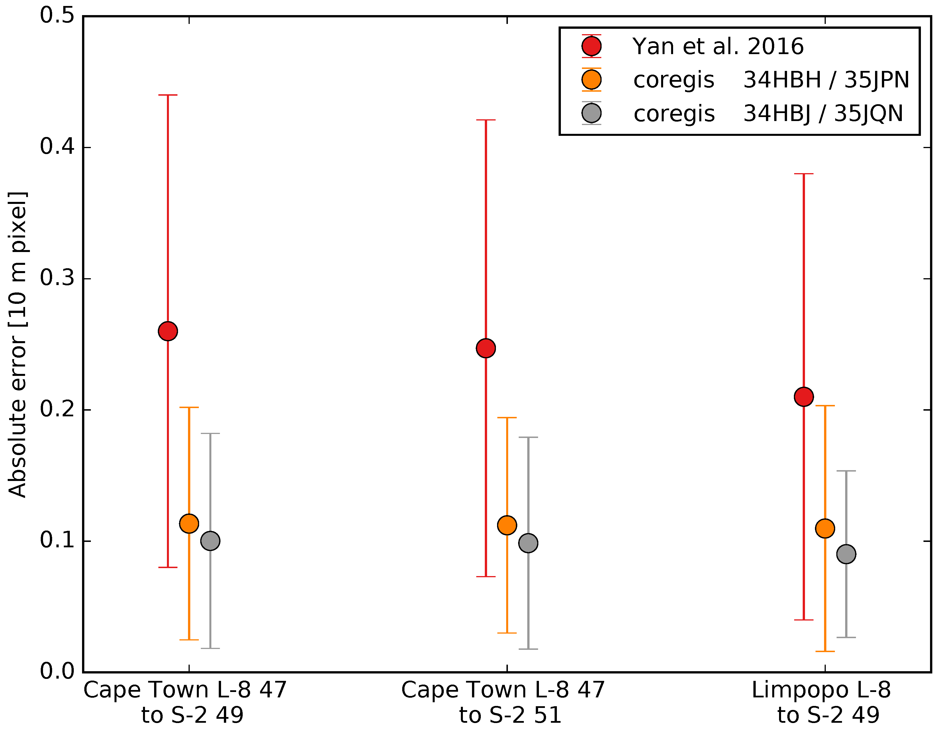
Figure 5.
Comparison of the co-registration RMSEs obtained after geometrical corrections with AROSICS and coregis for one of the Ukrainian test site (34UFU). (note, L-8: Landsat-8; S-2: Sentinel-2).
Figure 5.
Comparison of the co-registration RMSEs obtained after geometrical corrections with AROSICS and coregis for one of the Ukrainian test site (34UFU). (note, L-8: Landsat-8; S-2: Sentinel-2).

Figure 6.
Co-registration before and after corrections as a function of the time lag between the master image (31TGK, 23 August 2016) and the slave images.
Figure 6.
Co-registration before and after corrections as a function of the time lag between the master image (31TGK, 23 August 2016) and the slave images.

Figure 7.
Relationship between the before and after correction for the time-series (31TGK, master 23 August 2016). Due to two outliers the relationship is characterized by a low Pearson’s but shows a monotonic behaviour indicated by a high Spearman rank correlation .
Figure 7.
Relationship between the before and after correction for the time-series (31TGK, master 23 August 2016). Due to two outliers the relationship is characterized by a low Pearson’s but shows a monotonic behaviour indicated by a high Spearman rank correlation .

Figure 8.
Surface motion time-series for the Harmalière landslide from 5 May 2016 to 21 August 2017 at three selected points at (A) the head scarp, (B) the transport zone and (C) the toe. The figures show the measured velocities in relation to the background noise (95% quantile). Only measurements exceeding the respective background noise are taken into account to compute the cumulative displacement.

Figure 9.
Subset of the time-series of horizontal surface displacement fields for the Harmalière landslide from 5 May 2016 to 2 September 2019 and 11 December 2016 to 11 March 2017. The plots A to I show the acceleration and deceleration associated to the main reactivation end of June 2016. The plots J to K depict the period 11 December 2016 to 11 March 2017 with a further activation of the head scarp on 29 January 2017.

Figure 10.
Median and standard deviation of surface displacement fields for the Kaikoura earthquake (14 November 2016) computed from 4 pre-earthquake and 5 post-earthquake Sentinel-2 images (30 May 2016 to 4 May 2017). The plots A-D show the results without correction and the the plots E-G show the results after the correction illustrating that the striping artefacts are removed and that the measurement’s standard deviation is significantly reduced.

© 2018 by the authors. Licensee MDPI, Basel, Switzerland. This article is an open access article distributed under the terms and conditions of the Creative Commons Attribution (CC BY) license (http://creativecommons.org/licenses/by/4.0/).
Share and Cite
MDPI and ACS Style
Stumpf, A.; Michéa, D.; Malet, J.-P. Improved Co-Registration of Sentinel-2 and Landsat-8 Imagery for Earth Surface Motion Measurements. Remote Sens. 2018, 10, 160. https://doi.org/10.3390/rs10020160
AMA Style
Stumpf A, Michéa D, Malet J-P. Improved Co-Registration of Sentinel-2 and Landsat-8 Imagery for Earth Surface Motion Measurements. Remote Sensing. 2018; 10(2):160. https://doi.org/10.3390/rs10020160
Chicago/Turabian StyleStumpf, André, David Michéa, and Jean-Philippe Malet. 2018. "Improved Co-Registration of Sentinel-2 and Landsat-8 Imagery for Earth Surface Motion Measurements" Remote Sensing 10, no. 2: 160. https://doi.org/10.3390/rs10020160
Note that from the first issue of 2016, this journal uses article numbers instead of page numbers. See further details here.