Fusion of NASA Airborne Snow Observatory (ASO) Lidar Time Series over Mountain Forest Landscapes


Jet Propulsion Laboratory, California Institute of Technology, Pasadena, CA 91109, USA
*
Author to whom correspondence should be addressed.
Remote Sens. 2018, 10(2), 164; https://doi.org/10.3390/rs10020164
Submission received: 13 November 2017
/
Revised: 18 January 2018
/
Accepted: 22 January 2018
/
Published: 24 January 2018
(This article belongs to the Special Issue Mountain Remote Sensing)
Abstract
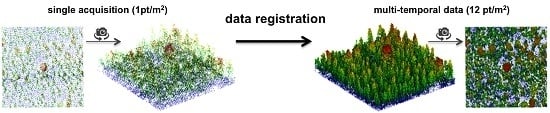
:Mountain ecosystems are among the most fragile environments on Earth. The availability of timely updated information on forest 3D structure would improve our understanding of the dynamic and impact of recent disturbance and regeneration events including fire, insect damage, and drought. Airborne lidar is a critical tool for monitoring forest change at high resolution but it has been little used for this purpose due to the scarcity of long-term time-series of measurements over a common region. Here, we investigate the reliability of on-going, multi-year lidar observations from the NASA-JPL Airborne Snow Observatory (ASO) to characterize forest 3D structure at a fine spatial scale. In this study, weekly ASO measurements collected at ~1 pt/m2, primarily acquired to quantify snow volume and dynamics, are coherently merged to produce high-resolution point clouds (12 pt/m2) that better describe forest structure. The merging methodology addresses the spatial bias in multi-temporal data due to uncertainties in platform trajectory and motion by collecting tie objects from isolated tree crown apexes in the lidar data. The tie objects locations are assigned to the centroid of multi-temporal lidar points to fuse and optimize the location of multiple measurements without the need for ancillary data or GPS control points. We apply the methodology to ASO lidar acquisitions over the Tuolumne River Basin in the Sierra Nevada, California, during the 2014 snow monitoring campaign and provide assessment of the fidelity of the fused point clouds for forest mountain ecosystem studies. The availability of ASO measurements that currently span 2013–2017 enable annual forest monitoring of important vegetated ecosystems that currently face ecological threads of great significance such as the Sierra Nevada (California) and Olympic National Forest (Washington).
1. Introduction
In the western US, snowmelt from mountains is the main source of water within a complex ecosystem that is rapidly changing due to frequent natural and socio-economic pressures over the past few decades [1,2]. In particular, mountainous ecosystems in the Sierra Nevada (California) are currently experiencing drastic disturbance and regeneration events such as tree mortality, fire, insect damage, disease, and drought [3]. The dynamic impacts of these processes are still not well known mainly due to the lack of long-term forest measurements characterizing 3D forest structure (e.g., forest height, vegetation vertical profile) changes over time and space. For instance, the uncertainty associated with the poor understanding of forest dynamics in terms of carbon fluxes in North America is nearly 50% [4].
Field inventory techniques are constrained by the spatial and temporal frequency of sampling and are not optimal for characterizing disturbance and regeneration processes, namely over mountain environments where the complex topography enhances heterogeneity on forest structure and creates access difficulties. Remote sensing techniques have been used to produce time-series of maps at regional- and landscape-level using medium- and high-resolution products such as Landsat and QuickBird (e.g., [5,6,7]). However, they are not adapted to characterize forest with the detail required to study many ecological processes such as shrubby vegetation fuel loads estimation, forest vertical profile characterization, and tree recruitment. Airborne lidar is the best tool to measure large swaths of forest structure at high spatial resolution in both vertical and horizontal dimensions. Its ability to characterize fine scale features such as tree counting or low vegetation density have been demonstrated over different ecosystems [8,9]. However, the high cost of airborne lidar acquisition has been a limitation to surveying large areas with reasonable temporal resolution in order to study forest disturbance and regeneration [10,11,12,13,14,15,16].
In this work, we investigate the reliability of fusing lower resolution but frequent lidar datasets acquired by the NASA-JPL Airborne Snow Observatory (ASO) to characterize the forest 3D structure at a fine scale. The ASO focus is the mountain snowpack and as such does not require high point densities that are needed to characterize forest canopies [17]. Instead, ASO offers multiple acquisitions over mountain systems each winter and spring in, at present, 12 mountain watersheds (Figure 1a) that are populated by vegetated areas of great ecological interest over the Sierra Nevada (California, since 2013), the Rocky Mountains (Colorado, since 2013), Mount Jefferson (Oregon, since 2016), and Mount Olympus (Washington, since 2014). With the multiple acquisitions each year, temporal sampling may be converted to an effective higher point density by the fusion of point clouds. Indeed, these datasets have the potential to be an important asset for the forest community in addition to its main purpose of mapping snowpack and snow melting.
Low point cloud densities (~1 pt/m2) have been successfully used in the framework of many applications (e.g., biomass estimates), but they require extensive field work to calibrate the signal [18,19]. On the contrary, high density point clouds (>8 pt/m2) allow direct extraction of forest metrics alleviating the need for costly and time-consuming field work [20,21], reduce uncertainty in forest metrics estimation (e.g., maximum and mean height of canopy) [22], and better represent understory and near-surface vegetation [23]. Therefore, we have the opportunity to markedly improve the forest structure characterization by coherently fusing the weekly ASO measurements (~1 pt/m2) in order to significantly increase the point density (up to ~12 pt/m2) and provide a multi-year dataset that is then optimal for any type of lidar-based assessment of vegetation. The multi-year ASO datasets can be readily compared and fused with other airborne and satellite datasets (e.g., hyperspectral imagery) in the framework of many applications such as species mapping or canopy water loss studies. Below, we present the methodology to compute a spatially coherent high-resolution point cloud from multiple lower-resolution surveys. We assess the spatial geolocation accuracy of individual lidar acquisitions in order to compensate for systematic bias to provide a final point cloud that meets the requirements in term of both geometry coherence and geolocation accuracy for fine-scale forestry studies.
Registering Lidar 3D Point Clouds
Lidar systems provide 3D point clouds with increasing accuracy and reliability. When the same area is measured multiple times, those point clouds can be fused to increase effective point density. However, the individual lidar point clouds must be co-registered to compensate for 3D shifts between the different acquisitions. Although ASO acquisition parameters do not change appreciably for a given study basin (e.g., flight lines path and flight altitude), lidar datasets can have planimetric shifts due to inaccuracies in platform trajectory estimation introduced by the GPS (Global Position System) receiver and drifts of the IMU (Inertial Measurement Unit) that are coupled to the lidar sensor.
Most registration methods for converting misaligned 3D point clouds to a single spatial geometry consist of two main steps: (1) the identification of corresponding objects in the different datasets, called “tie objects”, to calculate the spatial shift between point clouds, and (2) the establishment of a coordinate transformation model composed by a translation, a rotation, or by a combination of both to adjust the coordinates of the datasets according to the estimated spatial shift. Registration methods can be divided into four main families based on the approach used to identify tie objects: artificial reflective targets-based, features-based, surface-based, and point-based approaches. The first is the least sophisticated and involves artificial reflective targets that are placed along the study site. These targets are regarded as tie objects in two different datasets to calculate the transformation model parameters [24]. In the features-based approach, a collection of tie objects is first identified in each point cloud using automatic or semi-automatic methods. They rely heavily on the ability of the extraction method to accurately identify tie objects, which can be defined as (a) key points (e.g., electric poles location, [25]), (b) building corners [26], or specific patterns such as (c) spheres and cylinders [27] or even (d) segments and curves [28]. The surface-based methods extract tie objects using surface models (typically a mesh or a grid raster product such as a Delaunay Triangulation or a DTM, respectively) instead of using the original 3D point cloud. They usually focus on objects easily recognized such as depressions or cliff edges [29]. Finally, the point-based method does not rely on the extraction of tie objects. Instead, the parameters of the transformation model are calculated from the original point cloud. The most common approach for conducting this transformation is the Iterative Closest Point (ICP) algorithm that aligns two lidar point clouds by minimizing the distance between the corresponding closest neighborhoods [30].
Unfortunately, these existing registration methods are not immediately adaptable to fusing the ASO data due to three main reasons: (1) the lower spatial resolution of single ASO acquisitions, (2) the fact that the ASO covers natural environments where tie objects are difficult to extract, and (3) the dynamics of the landscape that change with snowfall, snow melt, and occurrence of ice at the surface. The lower point density of the ASO data limits the identification of well-defined key points that could be used as tie objects (e.g., top of the crowns or artificial reflecting targets) and limits the ICP method because the probability of a laser pulse hitting the same object (e.g., a tree crown apex or edge) over every acquisition is significantly low. In addition, the fact that we are working in a natural environment with very few human structures prevents us from applying feature-based approaches that use standard patterns (e.g., building corners) as tie points. Finally, the surface-based methods are not appropriate because distinctive landscape features may not be visible depending on snow and ice occurrence (such as terrain depressions, road intersections, and river outlines).
In this work, we (1) assess the quality of ASO lidar data in terms of geolocation accuracy, and (2) demonstrate a new method to register low-resolution point cloud data in order to calculate a spatially coherent, high-resolution point cloud. We implement the end-to-end processing approach on ASO acquisitions over a sample area in the Tuolumne River Basin, Sierra Nevada (California) and provide assessments of the performance of the approach for 3D characteristics of forest structure.
2. Material
2.1. Study Site
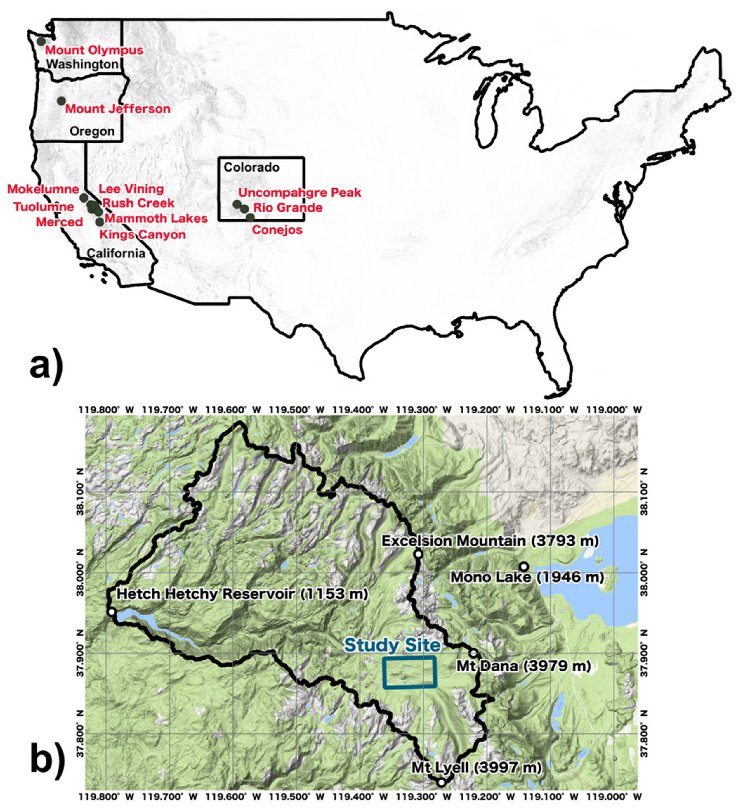
We use ASO data acquired over the Tuolumne River Basin on the west side of the Sierra Nevada, California, USA (Figure 1b). The Tuolumne Basin above the O’Shaughnessy Dam has ~1170 km2 area, of which ~60% is covered by forests of California red fir, Jeffrey pine, and Douglas fir. Elevations range from 1190 m at the dam up to 4000 m at the summit of Mt Lyell, the highest point in Yosemite National Park, which is situated at the southern end of the basin. The Tuolumne River Basin has been the site of numerous hydrological studies because it is one of the main sources of water supply for the state, in particular for the city of San Francisco [31,32].
California has a Mediterranean climate, where most precipitation falls between November and March, and approximately 75% of California’s annual precipitation comes from the high-elevation snowpack of the Sierra Nevada. The large climate variability in the maritime region impacts the precipitation and runoff fluctuations from year to year, which deviate from under 50% to over 200% of climatological averages [33]. The study area has been monitored by the ASO routinely since 2013 to capture these fluctuations in snow cover and runoff. This study is focused on a 7 km × 4 km site with significant vegetation cover located in the Tuolumne Meadows (blue rectangle in Figure 1b).
2.2. Lidar Data
In the following, we briefly describe the processing chain used by ASO to produce classified lidar point clouds (ground/off-ground points) that are georeferenced according to a global coordinate system [17]. We use data collected on 12 different dates in 2014 using the ASO Riegl Q1560 scanning lidar system in full-waveform mode. Eleven of the 12 datasets were acquired in snow-on conditions between March 23rd and June 5th and the last acquisition was during the summer (27 August) to map the surface elevation during snow-off conditions. The Q1560 uses dual 1064 nm wavelength lasers, with a scan angle of , and with a angle relative to the cross-track axis. The flight altitude was nominally 6550 m (21,500 ft MSL) with individual swath widths of ~4.3 km and a nominal pulse footprint size of 0.75 m at the high elevations to 1.5 m in the valleys and at low elevations. Full coverage of the Tuolumne river watershed requires 28 flight lines, and the study area (Figure 1b) requires only six flight lines. The position and orientation of the instrument platform on the aircraft are given by onboard GPS/IMU measurements. In addition, the onboard GPS measurements are calibrated using the Trimble RTX real-time differential position correction using a network of GPS base stations. The digitized waveforms are converted into lidar point clouds, with each laser pulse giving rise to 1–7 lidar returns [34]. The resulting point cloud is then converted into the WGS84/UTM zone 11N global coordinate system.
The data processing chain includes the identification of ground and off-ground points using the Multiscale Curvature Classification (MCC) algorithm [35]. Note that, within the lidar datasets acquired in snow-on condition, points classified as ground may correspond to the snowpack surface rather than the bare soil over snow-covered areas.
3. Methods
We developed a method to compute a normalized high-density point cloud data by coherently merging multiple lower-density lidar acquisitions. The method workflow is composed of three major processing steps, namely (1) point cloud registration, (2) snow surface points removal and GDT (Ground Delaunay Triangulation) recalculation, and (3) point cloud normalization (Figure 2). In the first step, we develop a new registration method to coherently merge individual point clouds. The method estimates both planimetric and altimetric discrepancies between individual acquisitions in order to establish a set of coordinate transformation models that are then applied to each point cloud to adjust their location. The registration method is explained in detail in Section 3.1.
The purpose of the second step is to iteratively produce a robust GDT to characterize the complex topography of the mountainous environment. To do this, we remove low lidar points from the snow-on acquisitions because they might correspond to the snowpack surface and would be confused with vegetation because they show higher elevation compared with the true GDT. First, we compute a GDT using the points classified as ground within the snow-off dataset. Then, we examine each of the snow-on acquisitions to remove points corresponding to the snowpack surface. In practice, we iteratively consider each triangle of the reference GDT in order to select the lidar points classified as ground which planimetric coordinates are located within the boundaries the triangle. Those points are removed from the dataset if their averaged vertical distance to the GDT is greater than 5 cm as this suggests that the area of the triangle is covered by snow. The remaining points are merged to the former point cloud and its GDT recalculated using the MCC algorithm [35]. We start this process with the lidar acquisitions that are more likely to contain the largest number of points representing the bare soil (e.g., 5 June 2014, Figure 2) in order to produce a denser and more accurate GDT in the earlier iterations. Note that we consider the existence of ground points within the datasets collected during snow-on conditions because the snowpack does not melt uniformly throughout the study site, leaving exposed patches with valid ground points. Finally, we remove the effect of topography from the high-resolution lidar data by interpolating each lidar point in the GDT in order to calculate its distance to the ground and calculate a normalized point cloud (Point cloud normalization step, Figure 2). The latter is a standard product in the framework of vegetation analysis because it allows direct retrieval of the height of vegetation from the point cloud.
3.1. Point Cloud Registration
The registration method is a feature-based approach that uses coniferous tree apexes as tie objects, as they are the most constant feature in the study area across time due to their conical shape and lack of snow accumulation. The tie objects are then used to establish a set of coordinate transformation models that apply to individual point clouds in order to compensate for geolocation inaccuracies between acquisitions. This allows us to coherently merge the individual acquisitions to create a high-density point cloud with a single geometry (Point cloud registration step, Figure 2). The transformation models follow
where and are the coordinates of the original and adjusted lidar point clouds, respectively; and where is the number of points in a given point cloud and is the number of lidar acquisitions; is a translation vector and a 3D rotation matrix defined by the axis angles . Our method is composed of three main steps: (1) definition of a set of tie objects (Figure 3a), (2) adjustment of the location of tie objects (Figure 3b), and (3) calculation of transformation models for each lidar acquisition (Equation (1)).
In the first step, we manually define a dataset of tie objects by identifying isolated tree crowns with well-defined apexes. To do this, we generate a 1 m resolution Digital Surface Model (DSM) by selecting the highest lidar point within each pixel from a point cloud composite computed by merging the lidar individual acquisitions before registration. This preliminary DSM identifies isolated tree crowns with reasonable accuracy despite the fact that it may have spatial inaccuracies due to misalignments between lidar acquisitions. Then, we define a circular neighborhood located over each tie object to select the corresponding highest lidar point from each acquisition. The later points are hereafter called vertices and they are defined by with , where s is the number of tie objects for a given study site. In Figure 3a, we show a dummy example of three lidar acquisitions and two tie objects (i.e., j = 1, 2, 3 and k = 1, 2; respectively). We set the maximum radius of the circular neighborhood to 5 m, as the spatial misalignment between acquisitions is expected to be less than 5 m. Furthermore, the use of a maximum 5 m neighborhood over isolated trees avoids the risk of selecting vertices that correspond to different tree crowns. Due to the lower density of ASO single acquisitions, it is likely that none of the vertices would correspond to the actual apex of the tie objects. Indeed, when considering lower density lidar acquisitions, we expect errors on the estimation of important forest metrics such as the location of trees and their maximum height (orange, cyan, and blue trees in Figure 3a).
In the second step, we adjust the location of the tie objects by assigning their positions to the centroid of the corresponding vertices. The tie objects location is here defined by , which is represented in Figure 3b the red cross. This allows us to calculate the locations of the adjusted tie objects as a function of each acquisition in order to ensure that the removal of outliers introduced by misalignment between flight lines are performed automatically without user decision in selecting the locations.
In the third step, we estimate a transformation model for each lidar acquisition defined as a function of the corresponding vertices () and centroids (). To do this, we set and in Equation (1) to estimate both the translation vector () and the rotation matrix () using a commonly used least-square fitting approach based on the singular value decomposition [36]. Note that we need at least four tie objects, i.e., , to solve the three-dimensional rigid model shown in Equation (1). However, a higher number of tie points would produce more robust transformation models.
Finally, we use and calculated for each lidar acquisition () in the previous step to compensate for location inaccuracies and calculate the adjusted point cloud coordinates as a function of the original coordinates (Equation (1)). Then, we merge the individual lidar acquisitions to obtain a high-density point cloud that contains points from all available acquisitions.
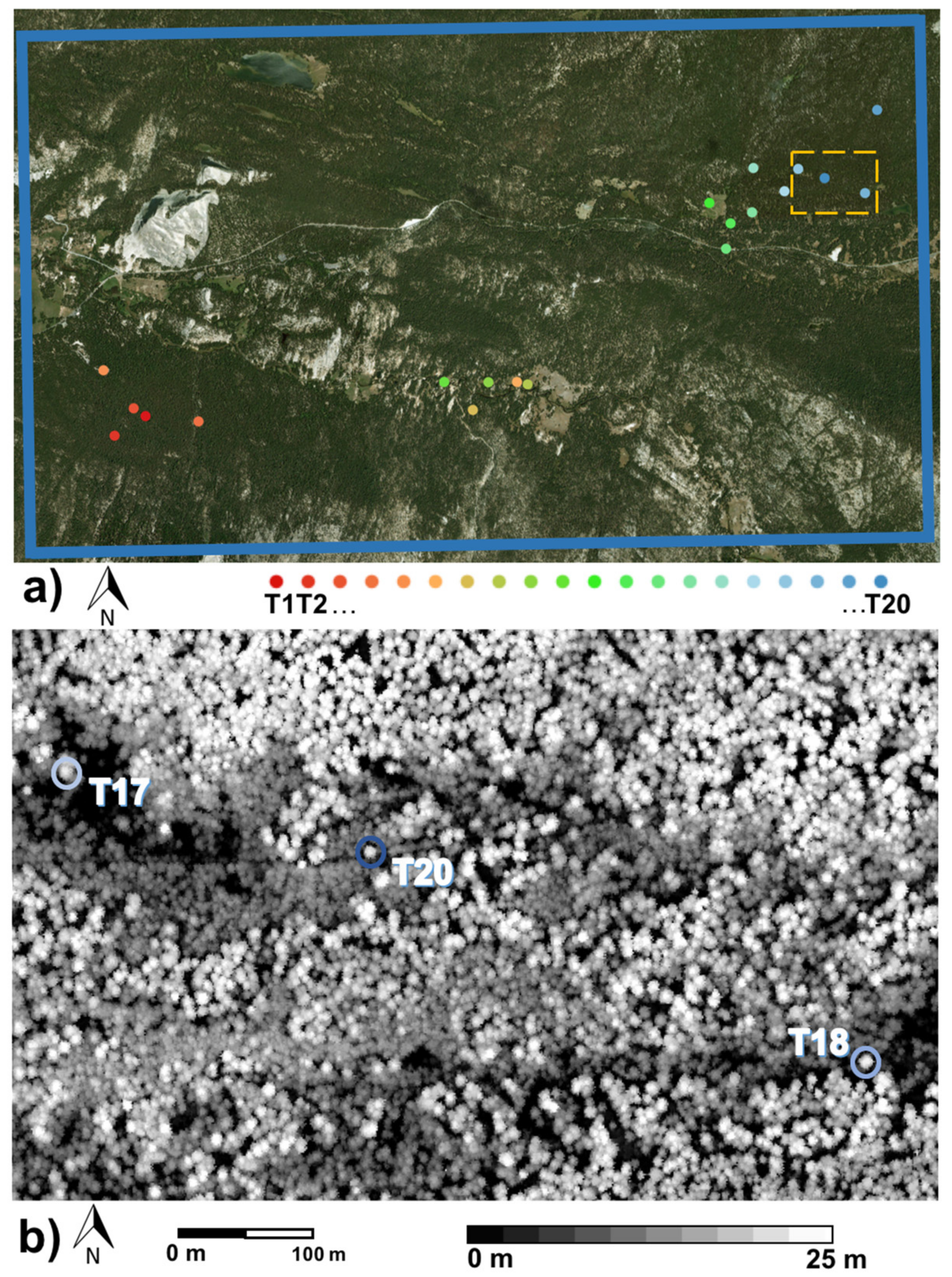
In this work, we selected twenty isolated trees for use as tie objects using a preliminary DSM distributed over the Tuolumne River basin study site (Figure 4).
3.2. Accuracy Assessment
The nature of the translation vectors () and rotation matrices () calculated for each lidar acquisition are indicators of the magnitude and direction of the misalignment between point clouds in terms of their geolocation. For a more intuitive comparison, we normalize the coordinates of the vertices as a function of the corresponding tie objects to compute scatter plots that provide visual and quantitative measures of systematic bias for each acquisition date (Figure 3c).
We start with that are the locations of the adjusted vertices calculated by applying Equation (1) on the original vertices () using the corresponding and . Then, we define and to reduce the differences in coordinates of the vertices (for both original and adjusted point clouds, respectively) by using the coordinates of the corresponding tie object. Finally, we calculate the centroid of the adjusted vertices to estimate the magnitude of the bias of each lidar acquisition. Figure 3c provides schematics that allow identification and quantification of systematic bias by comparing different lidar acquisitions. The magnitude of the bias can be interpreted directly from the coordinates of the centroids of the vertices as the coordinates of the corresponding tie objects have been transformed to match the origin of the graph (Figure 3c shows and not the original ).
4. Results and Discussion
Figure 5a shows the multiple lidar point clouds in the surroundings of tie object T1 (Figure 4a) before registration. In general, the point clouds from individual acquisitions are spatially consistent but as expected some forest features (e.g., the tree apexes) are not well defined in single acquisitions due to geolocation issues and low-density characteristics of the surveys that make the point cloud blurred. A demonstration of the adjustment method on the 3D point cloud composite is shown in Figure 5b when compared to Figure 5a, which shows the data after applying our registration approach. The improvements in terms of geometrical consistency are clear, particularly regarding the lidar acquisition that showed the largest bias (red dots). In addition, the main forest features such as the tree apexes are also markedly better defined in Figure 5b, suggesting that the location of remaining acquisitions have also been appropriately adjusted.
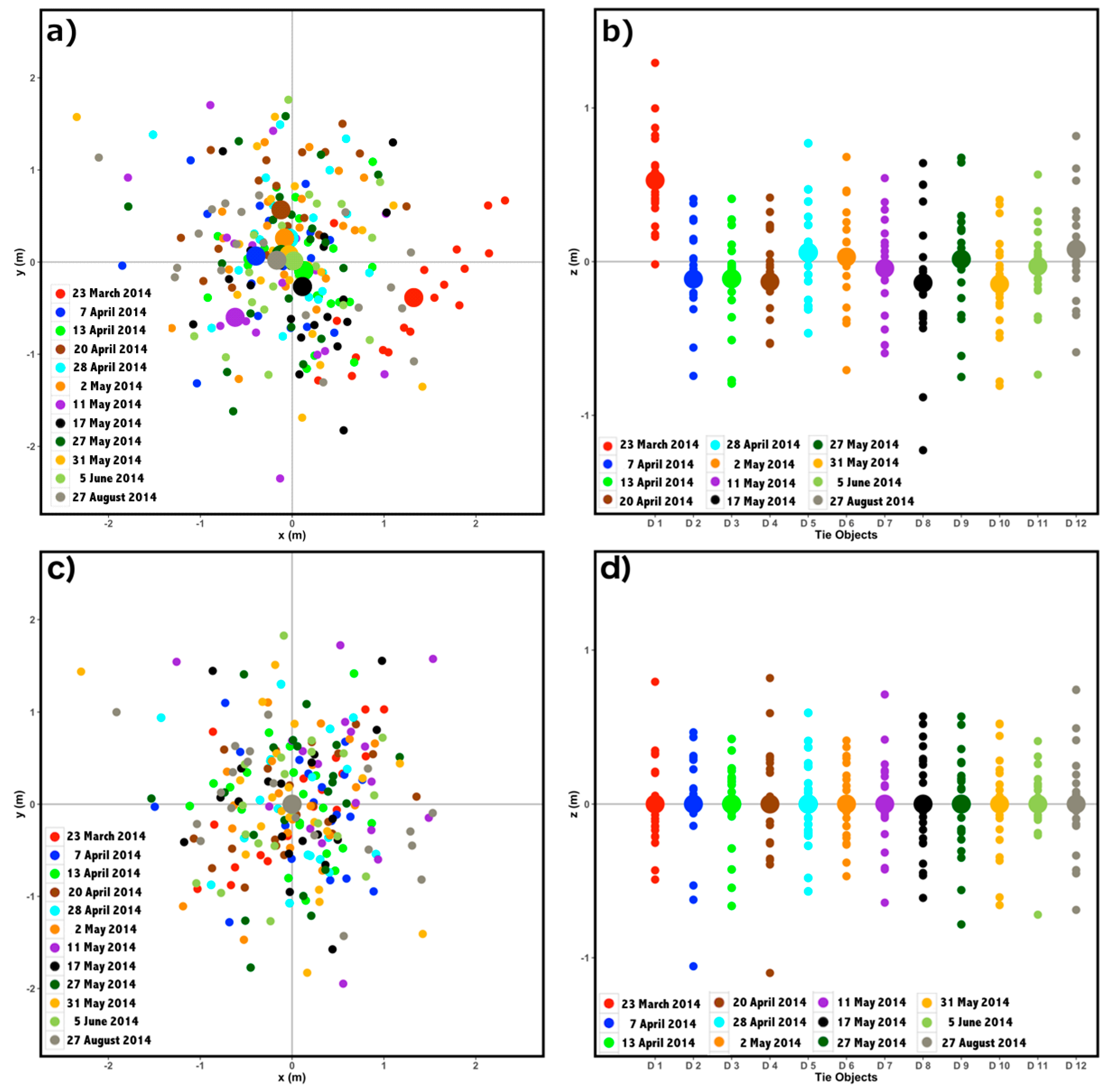
To quantify the misalignment between the lidar acquisitions and identify systematic bias, we normalize the multiple vertices using the corresponding tie object coordinates to draw a scatter plot similar to the one shown in Figure 3c. Results are show in Figure 6a,b, and supporting main statistics are summarized in Table 1. The distances between the vertices and the tie objects range between 0.02 m and 2.24 m with an average of 0.97 m in planimetry (horizontal displacement), whereas with respect to the altimetry (vertical displacement), they are within a smaller interval (0.00–1.52 m) and have a lower average (0.28 m). The accuracy of the original location of vertex-based metrics is not expected to be higher than these values due to the nature of the point cloud accumulation from lower density discrete returns that is subject to a low probability of the laser beam intersecting exactly the same feature of trees (e.g., tree apex). Despite the fact that the tree growth is small in severe climate conditions, the vertical errors might also be associated with the tree growth during Spring.
As discussed in the methods, the main goal of this work is not to compensate for local bias at the vertex level, which is not possible due to the lower resolution of the data. Instead, we aim to compensate for systematic biases at the individual acquisition level by means of the centroids locations calculated from the vertices (larger dots in Figure 6) and create an effective high-density characterization of the forest canopy. Figure 6a,b shows that the lidar acquisition on 23 March (represented by the red dots) has a larger geolocation systematic bias compared with the remaining ones in both horizontal and vertical dimensions (~1.3 m and ~0.53 m, respectively). The misalignment of the red dots corresponding to that particular acquisition is clearly visible in Figure 5a. The acquisition of May 11th (purple dots in Figure 6) has a moderate bias of 0.8 m in the horizontal dimension. The remaining centroids are relatively close to the origin of the graph even if the spread of the vertices is large (Figure 6a,b). Indeed, the average distance between the vertices and the tie objects (0.97 m and 0.28 m in the horizontal and vertical dimension, respectively) is larger than the average distance of the centroids (0.38 m and 0.12 m, respectively; Table 1). This means that although the mean distance between the vertices and the tie objects is high due to the fact the laser beam most likely missed the treetops, the centroid of the vertices is a reliable unbiased estimate of the tie object locations.
Figure 5c,d as well as Table 1 quantifies the improvements introduced by our method in terms of spatial consistency. As expected, all centroids overlap at the origin of the reference plane and confirm that our method is successful in removing the bias visible in the original measurements, which was of 0.38 m and 0.12 m in the horizontal and vertical domain, respectively (“centroid-based” columns in Table 1). While the centroid of the point cloud was modified, the spread of vertices changed little with respect to the original data. The average horizontal distance between the vertices and the corresponding tie objects decreased only from 0.97 m to 0.88 m when we compared the original and adjusted point clouds, (“vertex-based” columns in Table 1). Similarly, the averaged vertical distance decreased from 0.28 m to 0.25 m. Therefore, our approach does not force the vertices to individually converge toward the tie objects. Instead, it seeks a global solution that minimizes the distance between the entire number of vertices for a given acquisition—i.e., its centroid—and the corresponding tie object locations and, as such, preserves the original relative spatial geometry.
Figure 7a,b provide a perspective view of a single acquisition dataset and the high-density point cloud calculated by merging the registered individual acquisitions, respectively. The latter represents the forest structure at a finer resolution in both horizontal and vertical dimensions and enables the lidar forest inventory at the individual tree level, which is crucial for the monitoring of tree mortality as well as for tree biomass estimates over areas with non-existent field sampling [20,21]. Furthermore, the merging of multiple acquisitions improves mapping of the surface vegetation characteristics that highly impact the wildfire hazard and behavior [37,38].
Our methodology for the removal of snow points may eliminate some low vegetation points due to the fact that it is a conservative approach which is based only on the geometric and topological relationship between the lidar points and the reference ground Delaunay triangulation. We had considered to use additional information such as the lidar intensity to differentiate snowpack from low vegetation points [39]. However, it is difficult to isolate and normalize the energy reflected by the vegetation and the snow (or ground) in laser beams that give rise to multiple returns [40]. Moreover, the lidar intensity reflected by the snowpack is driven by many factors (e.g., content in impurities and liquid water) that change significantly across space and time [41] and, the incidence angle of the laser beam on the snowpack changes significantly that also introduces randomness in the lidar return intensity. Finally, the intensity would need to be calibrated for each lidar acquisition (e.g., using reflective reference targets) taking into account many factors such as the atmospheric conditions. On the one hand, our approach is readily transferable to different locations experiencing different weather conditions. On the other hand, the high temporal resolution of the ASO lidar measurements ensures that there are enough points to characterize the low vegetation properly, namely over areas of lower altitude where the snow melts earlier in spring and the shrubby vegetation is more luxurious due to milder climate conditions.
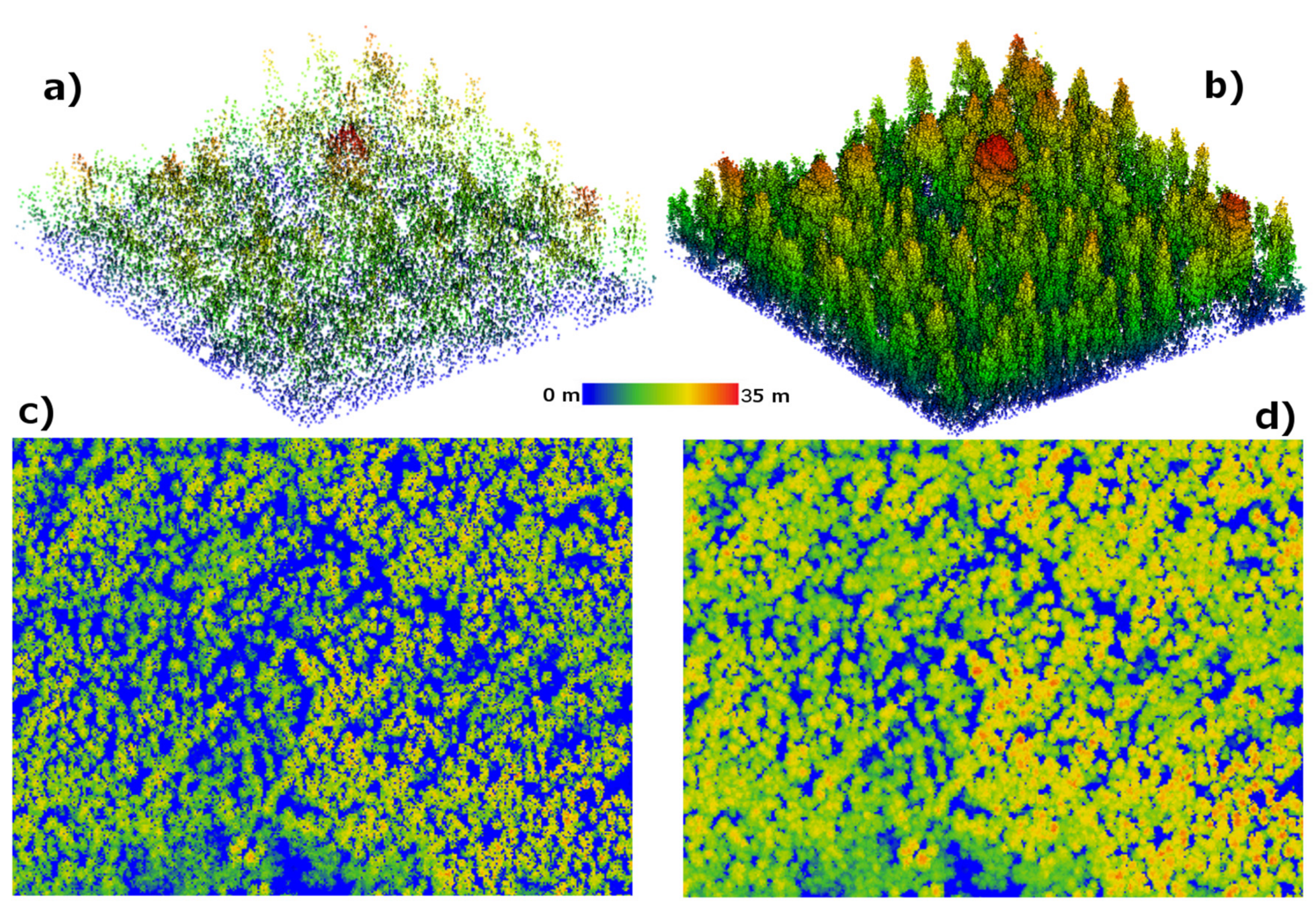
The improvements of the ASO multi-temporal data over single acquisitions can be readily shown in the calculation of the most commonly used product in forestry studies that is the canopy height model (CHM). In Figure 7, we show two CHM products derived from the ASO point cloud data with different point densities, providing clear distinctions in how the forest canopy is characterized with high point density data acquired from multiple acquisitions (Figure 7b,d) compared to a lower point density data from a single acquisition (Figure 7a,c). The results show that the successive ASO lidar acquisitions provide spatially consistent CHM to improve the characterization of the forest structure at fine resolution.
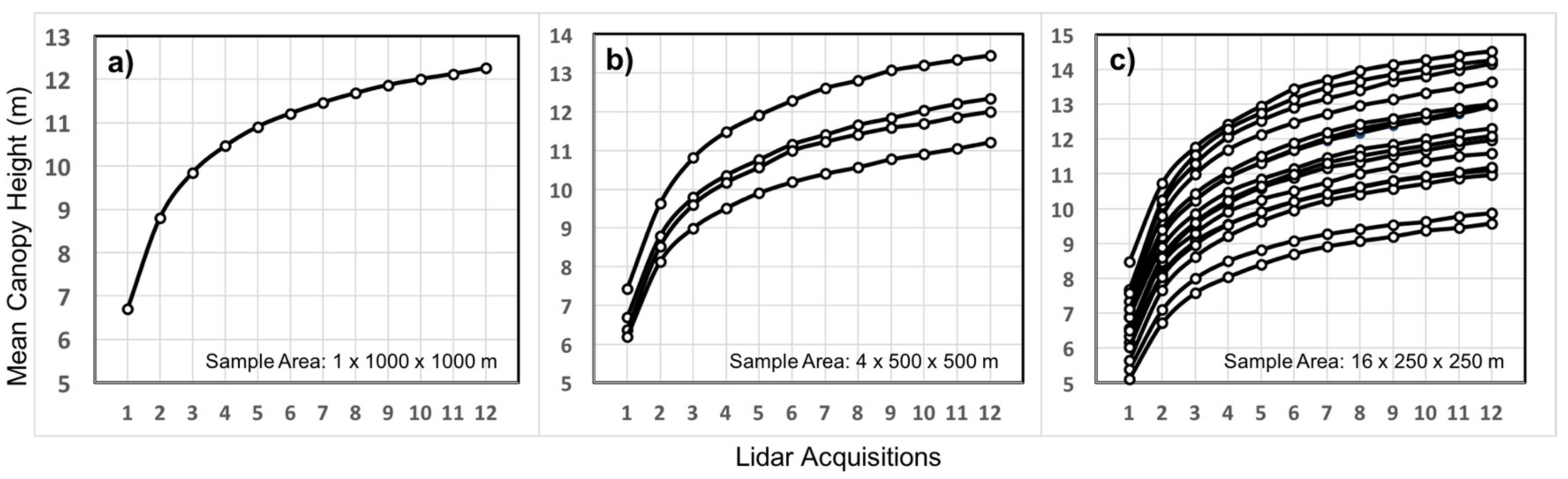
The impact of point density on the mean canopy height (MCH) was calculated using the CHM over an area of 1 km2 (1000 m × 1000 m, Figure 8a). On average at the 1 km2 scale, the mean canopy height increases by approximately a factor of 2 by adding 3–4 lidar acquisitions (Figure 8a: 1–5). Merging more acquisitions continues to improve MCH asymptotically with approximately 1 m increase by adding 6 more acquisitions (Figure 8a: 6–12). The results also suggest that the difference in point density introduces a significant bias (about 6 m) in height estimation that can be asymptotically reduced by adding more acquisitions. The bias in MCH can introduce a much larger bias when used in lidar-biomass allometric relations [42]. The improvement of MCH will also depend on the scale of analysis and may not follow the same asymptotic model as in Figure 8. To examine this, we performed the analysis at finer scales by dividing the 1 km2 sample area into four 500 m × 500 m (Figure 8b) and 16 250 m × 250 m subsample areas (Figure 8c). The results suggest that, depending on the landscape variations of forest structure and surface topography, the magnitude of bias and the asymptotic improvement with increasing point density may vary significantly.
Further detailed studies in mountain forest ecosystems with sparse vegetation are required to understand and quantify the impacts of point density and the number of acquisitions required to reach asymptotic improvements on forest structure and aboveground biomass estimation. However, our methodology for merging point density from different airborne lidar acquisitions has the potential to improve forest characteristics at scales of a single tree to landscape scales [21] and leverage the snowpack-motivated acquisitions to create an effective higher point density acquisition that can be used for analysis between actual higher density single acquisitions.
5. Conclusions
We provide a novel approach to combine a time series of snowpack-focused ASO lidar surveys to improve the characterization of ground surface and forest 3D structure. The nominal flights of the ASO for snowpack monitoring provide lower resolution datasets with limited capabilities for vegetation sampling, but its high temporal resolution (through multiple overpasses) enables the calculation of high-resolution point clouds by merging individual acquisitions annually. Our methodology first provides an assessment of the ASO lidar system reliability in terms of geolocation because it directly impacts the consistency of the high-density products. By combining 12 lidar acquisitions over a 7 × 4 km area in the Tuolumne River basin, we concluded that the ASO lidar system procedure that is used to georeference the data produces point clouds with reasonable geolocation accuracy. On average, we found an estimated bias of 0.38 m and 0.12 m with respect to the horizontal and vertical dimensions, respectively. However, certain single acquisitions show a systematic bias up to 1.38 m in planimetry (horizontal) and 0.53 m in altimetry (vertical). We show that our registration method is capable of identifying and compensating for systematic errors in order to improve the geometrical coherence of the point clouds composites.
Our point cloud registration method improved the location accuracy significantly by compensating for erroneous GPS/IMU measurements by averaging geolocation estimates of 12 lidar acquisitions. Our method was designed for application in dynamic natural landscapes with frequent snowfalls that make the selection of tie points very limited and is a unique aspect of the study. The most stable features in these landscapes are the top of tree crowns that play the role of tie objects in the methodology. Unlike former methods that offer a pair-wise solution (e.g., keeping one point cloud fixed as the reference geolocation data and the remaining point clouds are transformed to best match the reference), our approach uses tie objects that are calculated as the centroid using the multi-temporal data.
As a result, we register the point clouds as a function of an averaged location that can be used as a better proxy for the tree apex true location than a single GPS/IMU measurement. As such, our method applies an absolute registration (best compromise between a collection of objects and its UTM/WGS84 coordinates) rather than a relative registration (best match between corresponding points of two datasets). Therefore, the absolute co-registration has a clear advantage for analyzing multi-year point clouds because they can be directly compared. Moreover, our datasets can be directly compared with other sources of information such as aerial or satellite imagery. For instance, the merging of the ASO 3D forest characterization with airborne and satellite multispectral imagery enable the mapping of species, estimation of canopy water loss, and tree stress [43,44]. ASO offers a unique high-resolution lidar dataset to monitor forest and surface change over mountain ecosystems with complex ecological and hydrological processes while attending to its primary focus of characterizing mountain snowpack across large mountain basins.
Acknowledgments
We acknowledge support from the NASA Terrestrial Hydrology Program, NASA Applied Sciences, and the California Department of Water Resources. This work was performed at the Jet Propulsion Laboratory, California Institute of Technology under a contract with NASA.
Author Contributions
T.H.P. and K.J.B. as part of the ASO team designed and collected the lidar data; A.F., S.S., T.H.P., and K.J.B. conceived the idea of fusion the ASO data, and A.F. developed and implemented the methodology; A.F. wrote the paper; T.H.P., K.J.B., and S.S. participated in the editing of the writing.
Conflicts of Interest
The authors declare no conflict of interest.
References
- McIntyre, P.; Thorne, J.; Dolanc, C.; Flint, A.; Flint, L.; Kelly, M.; Ackerly, D. Twentieth-century shifts in forest structure in California: Denser forests, smaller trees, and increased dominance of oaks. Proc. Natl. Acad. Sci. USA 2015, 112, 1458–1463. [Google Scholar] [CrossRef] [PubMed]
- Meng, R.; Dennison, P.E.; Huang, C.; Moritz, M.A.; D’Antonio, C. Effects of fire severity and post-fire climate on short-term vegetation recovery of mixed-conifer and red fir forests in the Sierra Nevada Mountains of California. Remote Sens. Environ. 2015, 171, 311–325. [Google Scholar] [CrossRef]
- Potter, C.S. Satellite Image Mapping of Tree Mortality in the Sierra Nevada Region of California from 2013 to 2016. J. Biodivers. Manag. For. 2017, 6. [Google Scholar] [CrossRef]
- Thomas, N.E.; Huang, C.; Goward, S.N.; Powell, S.; Rishmawi, K.; Schleeweis, K.; Hinds, A. Validation of North American Forest Disturbance dynamics derived from Landsat time series stacks. Remote Sens. Environ. 2011, 115, 19–32. [Google Scholar] [CrossRef]
- Goward, S.N.; Masek, J.G.; Cohen, W.; Moisen, G.; Collatz, G.J.; Healey, S.; Houghton, R.A.; Huang, C.; Kennedy, R.; Law, B.; et al. Forest disturbance and North American carbon flux. EOS 2008, 89, 105–106. [Google Scholar] [CrossRef]
- Powell, S.L.; Cohen, W.B.; Kennedy, R.E.; Healey, S.P.; Huang, C. Observation of Trends in Biomass Loss as a Result of Disturbance in the Conterminous U.S.: 1986–2004. Ecosystems 2014, 17, 142–157. [Google Scholar] [CrossRef]
- Wang, X.; Huang, H.; Gong, P.; Biging, G.S.; Xin, Q.; Chen, Y.; Yang, J.; Liu, C. Quantifying multi-decadal change of planted forest cover using airborne LiDAR and Landsat imagery. Remote Sens. 2016, 8. [Google Scholar] [CrossRef]
- Morsdorf, F.; Marell, A.; Koetz, B.; Cassagne, N.; Pimont, F.; Rigolot, E.; Allgöwer, B. Discrimination of vegetation strata in a multi-layered Mediterranean forest ecosystem using height and intensity information derived from airborne laser scanning. Remote Sens. Environ. 2010, 114, 1403–1415. [Google Scholar] [CrossRef] [Green Version]
- Ferraz, A.; Mallet, C.; Jacquemoud, S.; Gonçalves, G.R.; Tomé, M.; Soares, P.; Pereira, L.G.; Bretar, F. Canopy Density Model: A New ALS-Derived Product to Generate Multilayer Crown Cover Maps. IEEE Trans. Geosci. Remote Sens. 2015, 53, 6776–6790. [Google Scholar] [CrossRef]
- Boehm, H.D.V.; Liesenberg, V.; Limin, S.H. Multi-temporal airborne LiDAR-survey and field measurements of tropical peat swamp forest to monitor changes. IEEE J. Sel. Top. Appl. Earth Obs. Remote Sens. 2013, 6, 1524–1530. [Google Scholar] [CrossRef]
- Kellner, J.R.; Asner, G.P. Winners and losers in the competition for space in tropical forest canopies. Ecol. Lett. 2014, 17, 556–562. [Google Scholar] [CrossRef] [PubMed]
- Meyer, V.; Saatchi, S.; Chave, J.; Dalling, J.; Bohlman, S.; Fricker, G.; Robinson, C.; Neumann, M.; Hubbell, S. Detecting tropical forest biomass dynamics from repeated airborne lidar measurements. Biogeosciences 2013, 10, 5421–5438. [Google Scholar] [CrossRef]
- Réjou-Méchain, M.; Tymen, B.; Blanc, L.; Fauset, S.; Feldpausch, T.R.; Monteagudo, A.; Phillips, O.L.; Richard, H.; Chave, J. Using repeated small-footprint LiDAR acquisitions to infer spatial and temporal variations of a high-biomass Neotropical forest. Remote Sens. Environ. 2015, 169, 93–101. [Google Scholar] [CrossRef] [Green Version]
- Blackburn, G.; Abd Latif, Z.; Boyd, D. Forest disturbance and regeneration: A mosaic of discrete gap dynamics and open matrix regimes? J. Veg. Sci. 2014, 25, 1341–1354. [Google Scholar] [CrossRef]
- Simonson, W.; Ruiz-Benito, P.; Valladares, F.; Coomes, D. Modelling above-ground carbon dynamics using multi-temporal airborne lidar: Insights from a Mediterranean woodland. Biogeosciences 2016, 13, 961–973. [Google Scholar] [CrossRef]
- Vepakomma, U.; St-Onge, B.; Kneeshaw, D. Response of a boreal forest to canopy gap openings—Assessing vertical and horizontal tree growth with multi-temporal lidar data. Ecol. Appl. 2011, 21, 99–121. [Google Scholar] [CrossRef] [PubMed]
- Painter, T.H.; Berisford, D.F.; Boardman, J.W.; Bormann, K.J.; Deems, J.S.; Gehrke, F.; Hedrick, A.; Joyce, M.; Laidlaw, R.; Marks, D.; et al. The Airborne Snow Observatory: Fusion of scanning lidar, imaging spectrometer, and physically-based modeling for mapping snow water equivalent and snow albedo. Remote Sens. Environ. 2016, 184, 139–152. [Google Scholar] [CrossRef]
- Jakubowski, M.K.; Guo, Q.; Kelly, M. Tradeoffs between lidar pulse density and forest measurement accuracy. Remote Sens. Environ. 2013, 130, 245–253. [Google Scholar] [CrossRef]
- Garcia, M.; Saatchi, S.; Ferraz, A.; Silva, C.; Ustin, S.; Koltunov, A.; Balzter, H. Impact of data model and point density on aboveground forest biomass estimation from airborne LiDAR. Carbon Balance Manag. 2017, 12. [Google Scholar] [CrossRef] [PubMed]
- Ferraz, A.; Saatchi, S.; Mallet, C.; Jacquemoud, S.; Gonçalves, G.; Silva, C.; Soares, P.; Tomé, M.; Pereira, L. Airborne Lidar Estimation of Aboveground Forest Biomass in the Absence of Field Inventory. Remote Sens. 2016, 8, 653. [Google Scholar] [CrossRef]
- Kandare, K.; Ørka, H.O.; Chan, J.C.; Dalponte, M. Effects of forest structure and airborne laser scanning point cloud density on 3D delineation of individual tree crowns. Eur. J. Remote Sens. 2016, 49, 1–23. [Google Scholar] [CrossRef]
- Roussel, J.-R.; Caspersen, J.; Béland, M.; Thomas, S.; Achim, A. Removing bias from LiDAR-based estimates of canopy height: Accounting for the effects of pulse density and footprint size. Remote Sens. Environ. 2017, 198, 1–16. [Google Scholar] [CrossRef]
- Ferraz, A.; Bretar, F.; Jacquemoud, S.; Gonçalves, G.; Pereira, L.; Tomé, M.; Soares, P. 3-D mapping of a multi-layered Mediterranean forest using ALS data. Remote Sens. Environ. 2012, 121, 210–223. [Google Scholar] [CrossRef]
- Bienert, A.; Maas, H. Methods for the Automatic Geometric Registration of Terrestrial Laser Scanner Point Clouds in Forest Stands. ISPRS Int. Arch. Photogramm. Rem. Sens. Spat. Inf. Sci. 2009, XXXVIII-3/W8, 93–98. [Google Scholar]
- Weinmann, M.; Weinmann, M.; Hinz, S.; Jutzi, B. Fast and automatic image-based registration of TLS data. ISPRS J. Photogramm. Remote Sens. 2011, 66, S62–S70. [Google Scholar] [CrossRef]
- Thirion, J.-P. New feature points based on geometric invariants for 3D image registration. Int. J. Comput. Vis. 1996, 18, 121–137. [Google Scholar] [CrossRef]
- Frome, A.; Huber, D.; Kolluri, R.; Bülow, T.; Malik, J. Recognizing Objects in Range Data Using Regional Point Descriptors. In Proceedings of the 8th European Conference on Computer Vision—ECCV 2004, Prague, Czech, 11–14 May 2004. [Google Scholar]
- Stein, F.; Medioni, G. Structural indexing: Efficient 3-D object recognition. IEEE Trans. Pattern Anal. Mach. Intell. 1992, 14, 125–145. [Google Scholar] [CrossRef]
- Chui, H.; Rangarajan, A.; Zhang, J.; Leonard, C. Unsupervised learning of an Atlas from unlabeled point-sets. IEEE Trans. Pattern Anal. Mach. Intell. 2004, 26, 160–172. [Google Scholar] [CrossRef] [PubMed]
- Gressin, A.; Mallet, C.; Demantké, J.; David, N. Towards 3D lidar point cloud registration improvement using optimal neighborhood knowledge. ISPRS J. Photogramm. Remote Sens. 2013, 79, 240–251. [Google Scholar] [CrossRef]
- Henn, B.; Clark, M.P.; Kavetski, D.; McGurk, B.; Painter, T.H.; Lundquist, J.D. Combining snow, streamflow, and precipitation gauge observations to infer basin-mean precipitation. Water Resour. Res. 2016, 52, 8700–8723. [Google Scholar] [CrossRef]
- Bair, E.H.; Rittger, K.; Davis, R.E.; Painter, T.H.; Dozier, J. Validating reconstruction of snow water equivalent in California’s Sierra Nevada using measurements from the NASAAirborne Snow Observatory. Water Resour. Res. 2016, 52, 8437–8460. [Google Scholar] [CrossRef]
- Lundquist, J.D.; Dettinger, M.D.; Cayan, D.R. Snow-fed streamflow timing at different basin scales: Case study of the Tuolumne River above Hetch Hetchy, Yosemite, California. Water Resour. Res. 2005, 41, 1–14. [Google Scholar] [CrossRef]
- RiANALYZE. Available online: http://www.riegl.com/products/software-packages/rianalyze/ (accessed on 8 July 2017).
- Evans, J.S.; Hudak, A.T. A multiscale curvature algorithm for classifying discrete return LiDAR in forested environments. IEEE Trans. Geosci. Remote Sens. 2007, 45, 1029–1038. [Google Scholar] [CrossRef]
- Arun, K.; Huang, T.; Blostein, S. Least-Squares Fitting of Two 3-D Point Sets. IEEE Trans. Pattern Anal. Mach. Intell. 1987, PAMI-9, 698–700. [Google Scholar] [CrossRef] [PubMed]
- Finney, M. FARSITE: Fire Area Simulator-Model Development and Evaluation; Department of Agriculture, Forest Service, Rocky Mountain Research Station: Ogden, UT, USA, 2004. [Google Scholar]
- Andrews, P.L. Current status and future needs of the BehavePlus Fire Modeling System. Int. J. Wildl. Fire 2014, 23, 21–33. [Google Scholar] [CrossRef]
- Wagner, W.; Hollaus, M.; Briese, C.; Ducic, V. 3D vegetation mapping using small-footprint full-waveform airborne laser scanners. Int. J. Remote Sens. 2008, 29, 1433–1452. [Google Scholar] [CrossRef]
- Yan, W.; Shaker, A.; Habib, A.; Kersting, A. Improving classification accuracy of airborne LiDAR intensity data by geometric calibration and radiometric correction. ISPRS J. Photogramm. Remote Sens. 2012, 67, 35–44. [Google Scholar] [CrossRef]
- Deems, J.S.; Painter, T.H.; Finnegan, D.C. Lidar measurement of snow depth: A review. J. Glaciol. 2013, 59, 467–479. [Google Scholar] [CrossRef]
- Lefsky, M.; Harding, D.; Keller, M.; Cohen, W.; Carabajal, C.; Del Bom Espirito-Santo, F.; Hunter, M.; de Oliveira, R. Estimates of forest canopy height and aboveground biomass using ICESat. Geophys. Res. Lett. 2005, 32, L22S02. [Google Scholar] [CrossRef]
- Swatantran, A.; Dubayah, R.; Roberts, D.; Hofton, M.; Blair, J.B. Mapping biomass and stress in the Sierra Nevada using lidar and hyperspectral data fusion. Remote Sens. Environ. 2011, 115, 2917–2930. [Google Scholar] [CrossRef]
- Asner, G.P.; Brodrick, P.G.; Anderson, C.B.; Vaughn, N.; Knapp, D.E.; Martin, R.E. Progressive forest canopy water loss during the 2012–2015 California drought. Proc. Natl. Acad. Sci. USA 2015, 2015, 201523397. [Google Scholar] [CrossRef] [PubMed]
Figure 1.
(a) Airborne Snow Observatory (ASO) coverage sites (black dots) across the US overlapped to a ASTER SRTM hillshade map. In (b) we focus on the Tuolumne River basin (Sierra Nevada, Central California) study site (the black polygon), which is overlapping a 10 m resolution DEM from the USGS National Elevation Dataset (NED) provided by Google Earth (Tuolumne River basin, 37°52′32.16″N, 119°20′08.85″W, http://www.earth.google.com (26 May 2014)). Well known locations such as Mono Lake, Mount Dana, and Excelsior Mountain are provided for better location. The study site (7 km × 4 km) is represented by the blue rectangle.

Figure 2.
Method workflow to calculate the normalized high-density point cloud from multi-temporal low-resolution data. GDT stand for Ground Delaunay Triangulation. Method steps are represented by the gray rectangles.
Figure 2.
Method workflow to calculate the normalized high-density point cloud from multi-temporal low-resolution data. GDT stand for Ground Delaunay Triangulation. Method steps are represented by the gray rectangles.
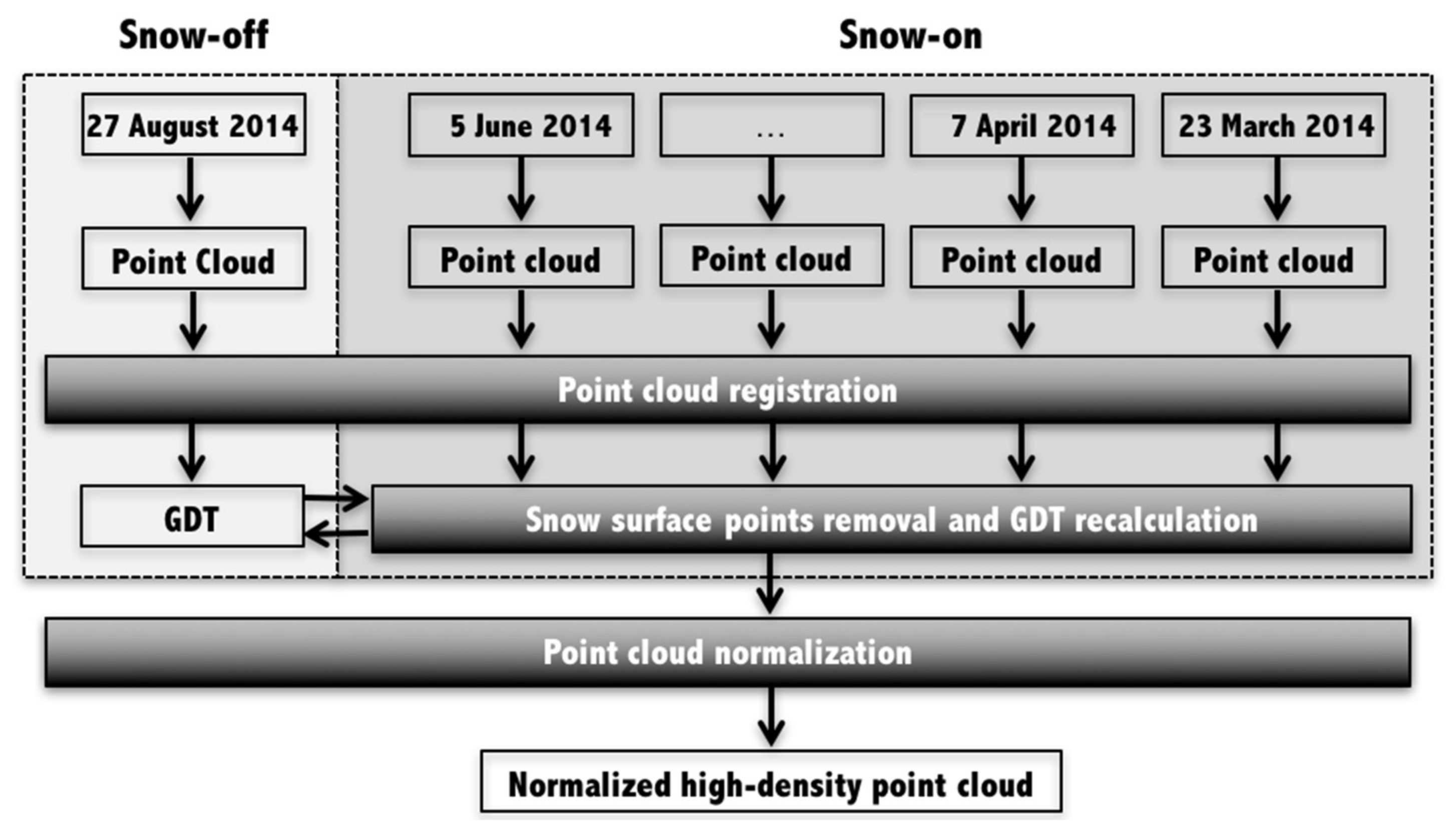
Figure 3.
Schematic of the lidar registration methodology showing (a) two isolated trees selected as tie objects (green trees referred as T1 and T2) and the highest lidar points (called vertices) from three different lidar acquisitions (referred as A1, A2, and A3) that define the location of the corresponding trees (orange, cyan and blue trees), which are offset from the apex of the tie object, (i.e., the green tree in the foreground). In (b), we represent the location of the original vertices and corresponding centroids (red cross) that are used to calculated the adjusted (or registered) vertices. The colored large semi-transparent circles follow the colors in (a) and represent the trees from an aerial view. The diameter of the circles is figurative and has no physical meaning. In (c), we show the coordinates of the adjusted vertices and corresponding centroids that are reduced to a local referential (with origin in (0,0)). The coordinates of the centroid give us an estimation of the magnitude and direction of the misalignment for each lidar acquisition (please refer to Section 3.2 for details regarding (c).
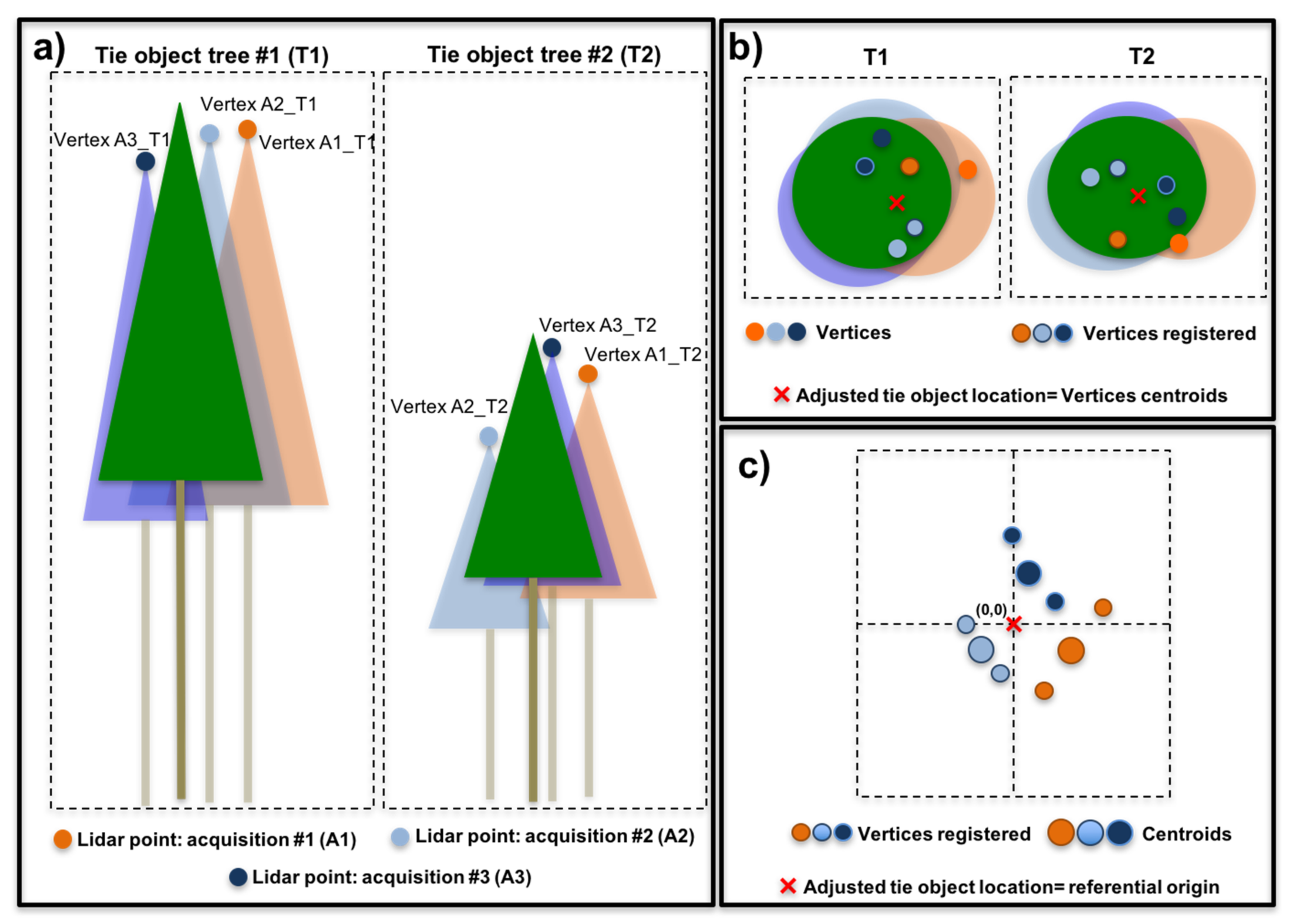
Figure 4.
Tuolumne River basin (a) study site (7 km × 4 km) that corresponds to the blue polygon in Figure 1b and the 20 tie objects trees (T1, T2, …, T20) selected for point cloud registration purposes represented by the colored dots and, (b) focus on the orange rectangle in (a) to show three tie object examples over a canopy height model. The colorbar in panel (b) corresponds to the vegetation height.

Figure 5.
Point cloud composites around tie object T1 (Figure 4a) (a) before and (b) after the registration of the individual datasets. Colors correspond to acquisition dates. The x and y axis correspond to the UTM coordinates and ellipsoidal altitude, respectively.
Figure 5.
Point cloud composites around tie object T1 (Figure 4a) (a) before and (b) after the registration of the individual datasets. Colors correspond to acquisition dates. The x and y axis correspond to the UTM coordinates and ellipsoidal altitude, respectively.
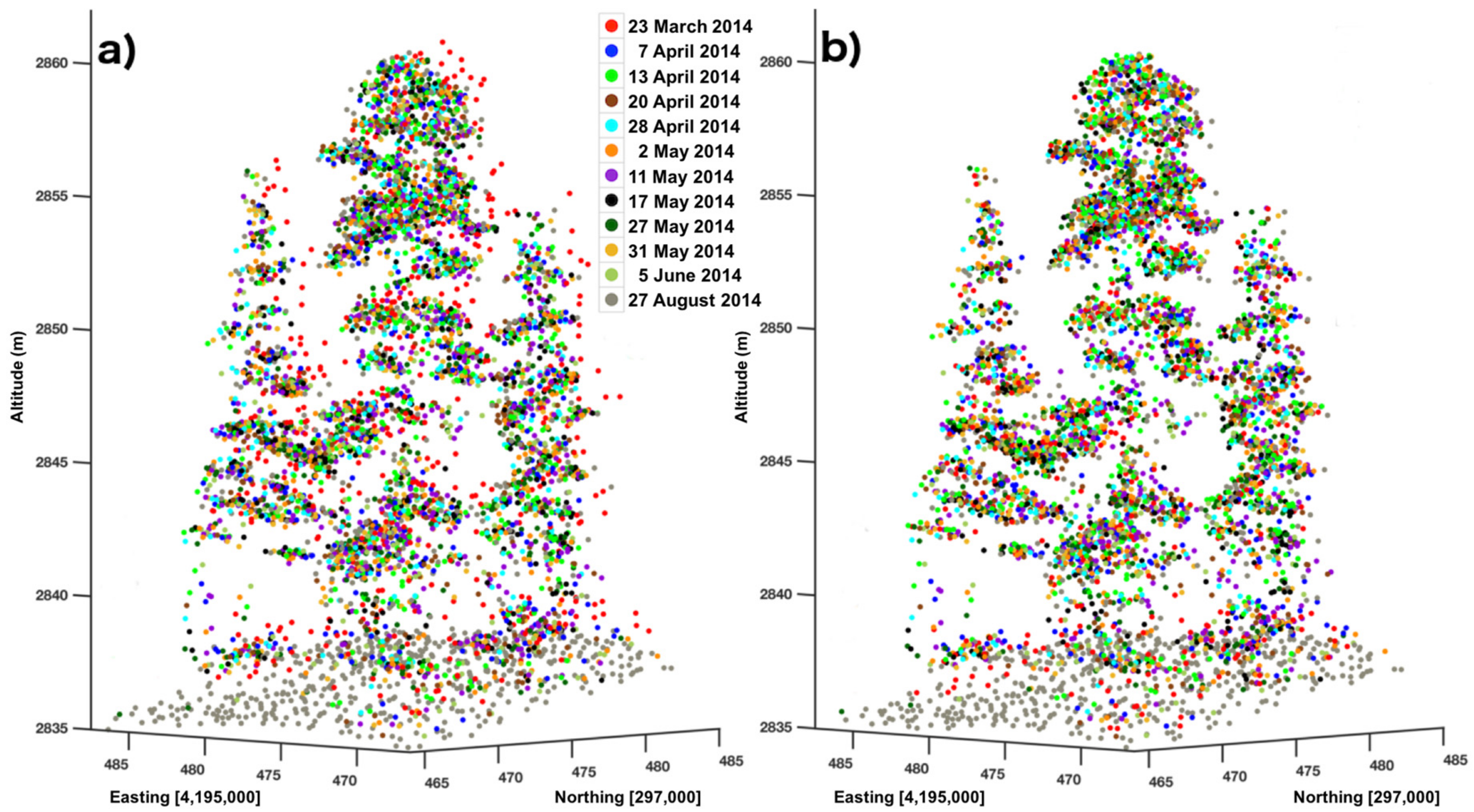
Figure 6.
Vertices grouped by acquisition date (small dots) and corresponding centroids (large dots) before (a,b) and after (c,d) registering the point clouds in the horizontal (a,c) and vertical (b,d) dimensions. The coordinates of the vertices represent the distance and direction with respect to the corresponding tie object in planimetry and altimetry (refer to Figure 3c). The centroids correspond to the average distance values for each lidar acquisition and are indicators of their systematic bias. Due to the fact that the bias has been removed by our co-registration method, the centroids of the vertices in (c,d) are located over the origin of the corresponding reference (0,0).

Figure 7.
Point cloud calculated (100 m × 100 m) using (a) lower-density single acquisition and (b) a high-density multi-temporal point cloud after co-registration. The canopy height models (1 m resolution, 350 m × 250 m) have been calculated using (c) one and (d) 12 lidar acquisitions.
Figure 7.
Point cloud calculated (100 m × 100 m) using (a) lower-density single acquisition and (b) a high-density multi-temporal point cloud after co-registration. The canopy height models (1 m resolution, 350 m × 250 m) have been calculated using (c) one and (d) 12 lidar acquisitions.

Figure 8.
Mean canopy height (MCH) calculated using a canopy height model (CHM) derived from increasing lidar acquisitions over area of 1000 m × 1000 m, showing (a) differences over the entire area, (b) when divided into four subsamples (at 500 m × 500 m), and (c) when divided further in 16 subsamples (at 250 × 250 m). The graphs shown are computed by averaging the values calculated by shuffling the order of lidar acquisitions (1–12) five times to remove the impact of eventual bias (e.g., tree growth).

Table 1.
Main statistics to summarize the graphs show in Figure 6a,b (original point cloud), c, and d (adjusted point cloud). The “vertex-based” columns refer to the distance between the vertices and the corresponding tie objects. The “centroid-based” columns refer to the distance between the centroids and the tie objects. All rows of the last two columns equal zero because the tie object location overlaps the centroid of the vertices. P and A stand for Planimetric and Altimetric dimensions.
| Original Point Cloud | Adjusted Point Cloud | |||||||
|---|---|---|---|---|---|---|---|---|
| Vertex-Based | Centroid-Based | Vertex-Based | Centroid-Based | |||||
| P | A | P | A | P | A | P | A | |
| mean (m) | 0.97 | 0.28 | 0.38 | 0.12 | 0.88 | 0.25 | 0.00 | 0.00 |
| max (m) | 2.24 | 1.52 | 1.38 | 0.53 | 2.10 | 1.10 | 0.00 | 0.00 |
| min (m) | 0.02 | 0.00 | 0.02 | 0.02 | 0.02 | 0.00 | 0.00 | 0.00 |
| sd (m) | 0.94 | 0.26 | 0.39 | 0.14 | 0.87 | 0.20 | 0.00 | 0.00 |
© 2018 by the authors. Licensee MDPI, Basel, Switzerland. This article is an open access article distributed under the terms and conditions of the Creative Commons Attribution (CC BY) license (http://creativecommons.org/licenses/by/4.0/).
Share and Cite
MDPI and ACS Style
Ferraz, A.; Saatchi, S.; Bormann, K.J.; Painter, T.H. Fusion of NASA Airborne Snow Observatory (ASO) Lidar Time Series over Mountain Forest Landscapes. Remote Sens. 2018, 10, 164. https://doi.org/10.3390/rs10020164
AMA Style
Ferraz A, Saatchi S, Bormann KJ, Painter TH. Fusion of NASA Airborne Snow Observatory (ASO) Lidar Time Series over Mountain Forest Landscapes. Remote Sensing. 2018; 10(2):164. https://doi.org/10.3390/rs10020164
Chicago/Turabian StyleFerraz, António, Sassan Saatchi, Kat J. Bormann, and Thomas H. Painter. 2018. "Fusion of NASA Airborne Snow Observatory (ASO) Lidar Time Series over Mountain Forest Landscapes" Remote Sensing 10, no. 2: 164. https://doi.org/10.3390/rs10020164
Note that from the first issue of 2016, this journal uses article numbers instead of page numbers. See further details here.