Sea Surface Current Estimation Using Airborne Circular Scanning SAR with a Medium Grazing Angle


1
National Laboratory of Radar Signal Processing, Xidian University, Xi’an 710071, China
2
Academy of Space Electronic Information Technology, Xi’an 710100, China
*
Author to whom correspondence should be addressed.
Remote Sens. 2018, 10(2), 178; https://doi.org/10.3390/rs10020178
Submission received: 19 November 2017
/
Revised: 15 January 2018
/
Accepted: 15 January 2018
/
Published: 26 January 2018
(This article belongs to the Special Issue Ocean Surface Currents: Progress in Remote Sensing and Validation)
Abstract
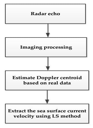
:Circular scanning synthetic aperture radar (SAR) is a novel imaging mode wherein the radar antenna rotates from 0 degrees to 360 degrees along the platform flight direction, providing us with a potentially effective technique to estimate the sea surface current velocity. In this paper, we propose a novel method to estimate the sea surface current velocity utilizing the Doppler centroid shifts of different scan angles over 360 degrees after the airborne platform motion compensation. In this method, the Doppler centroid shifts of the sea clutter at different scan angles are first extracted, and the corresponding compensation errors caused by the azimuth pointing and the incidence angle of the radar beam are considered. Finally, the least squares (LS) technique is applied to estimate the along-track velocity component and the cross-track velocity component of the sea surface current. The effectiveness of the proposed method is verified by the real data recorded by an airborne circular scanning SAR system.
1. Introduction
As an all-time and all-weather advanced modern sensing technique, the microwave remote sensing of the sea surface plays a very important role in the monitoring of the ocean environment because of its high spatial resolution and has drawn much attention in recent years. In the open sea, the sea surface current is an important factor for practical applications, such as climate forecasting, ocean environment surveillance, vessel navigation, etc. [1]. Therefore, the capability to precisely measure the sea surface current velocity would be a very useful and desired development.
The sea surface velocity consists of the sea surface current velocity, the phase velocity of the Bragg resonant waves, and the orbital velocity of the long waves [2,3,4]. The sea surface current can flow stably along a fixed direction over a certain scope of the sea surface. The spatial scale of the sea surface current varies from 1 km to 100 km, and can even reach several thousand kilometers. To date, some radar techniques have been utilized to measure the sea surface current velocity. The Bragg scattering theory specifies that the radar is primarily sensitive to radially-traveling waves that satisfy the Bragg resonant condition, and the phase velocity of the Bragg resonant waves is also stable. Therefore, the high-frequency (HF) ocean surface current radar can measure the sea surface current velocity utilizing the Bragg scattering theory of the sea surface [5,6,7,8] and can be applied to estimate the sea surface current velocity of large areas; for example, the shore-based HF ocean surface current radar of the University of Miami has been used to measure the 2-D offshore surface current vectors from 1.2 km to approximately 45 km resolutions [5].
For a spaceborne or airborne radar system, the radial velocity of the sea surface projection to the radar line-of-sight direction is measured by the Doppler shift caused by the movement of the sea surface obtained by the difference between the estimated Doppler centroid shift of the real data and the predicted Doppler centroid shift [9,10,11,12,13]. ENVISAT’s Advanced SAR has been used to estimate the sea surface current velocities with different resolutions by applying the median Doppler shift of radar echoes [9]. However, only the radial velocity of the sea surface is measured, and the three velocity components of the sea surface cannot be well distinguished such that the sea surface current velocity cannot be effectively extracted. Today, a well-established technology for the sea surface current estimation is represented by the X-band marine radar, both coherent [14,15] and non-coherent [16,17,18].
Recently, along-track interferometric (ATI) SAR has been widely applied to estimate the sea surface speed [19,20,21,22], which is measured by the phase difference of two antennas installed along the aircraft flight track (along-track) direction. However, ATI SAR can only extract the line-of-sight velocity of the sea surface and cannot effectively obtain the sea surface current velocity. Since the ATI SAR can only measure the overlapping area of the two SAR images, to overcome this limitation, the dual-beam ATI SAR has been developed. The dual-beam radar system employs an along-track pair of dual-beam antennas, and each antenna produces a forward beam and an aft beam [23,24] so that the along-track velocity component and the cross-track velocity component of the sea surface can be measured. Meanwhile, to distinguish the sea surface current velocity and the phase velocity of the Bragg resonant waves, multiple-frequency (L- and C-Band) ATI SAR [25] has been explored to estimate the sea surface current velocity, but the SAR system and the signal processing are more complicated. In addition, the microwave scatterometer has been used to monitor the sea surface current. The pencil-beam rotating scatterometer has been used to measure the sea surface current velocity [26], and the along-track velocity component and the cross-track velocity component of the sea surface current have been measured by the interferometric phases of the successive echoes of the two observational azimuths. However, the system requires a large antenna and a high pulse repetition frequency (PRF).
In this paper, we mainly explore the estimation method of the sea surface current velocity utilizing the circular scanning SAR technique based on the conical rotating microwave scatterometer. For the airborne circular scanning SAR, the platform flight height reaches several kilometers at the median grazing angles, and the measured range of the sea surface current extends from several kilometers to a few tens of kilometers. First, the algorithm extracts the Doppler centroid shifts of the different scan angles over 360 degrees, and the azimuth pointing error and the incidence angle error of radar system are considered to precisely estimate the sea surface current velocity. Then, the along-track and cross-track velocities of the sea surface current can be estimated by the LS method. The effectiveness of the proposed method has been evaluated by comparing it with a method presented in Toporkov et al. [23]. As a result, the proposed method allows us to improve the estimation precision of the sea surface current velocity.
The remainder of the paper is organized as follows: Section 2 analyzes the operational mode of the airborne circular scanning SAR. In Section 3, we present the analysis of the Doppler error caused by the platform motion and the estimation method of the sea surface current velocity. In Section 4, the estimation method is verified using real data from the airborne circular scanning SAR with different scan angles. In Section 5, the relevant conclusions are given.
2. Operational Mode of Airborne Circular Scanning SAR
In this section, we mainly analyze the operational mode of the airborne circular scanning SAR [27], and the scanning geometry of the airborne circular scanning SAR system is depicted schematically in Figure 1. As shown in Figure 1, the airborne platform flies along the horizontal plane x axis (along-track direction); the y axis (cross-track direction) is perpendicular to the x axis at the sea surface, and the aircraft is moving at a constant speed in a straight line. The antenna beam is, successively, in anticlockwise or clockwise rotation with a constant speed along the flight direction of the airborne platform using the mechanical rotating antenna or the phase control array antenna. is the incidence angle of the central slant range and is always kept at a constant value. The variable represents the azimuth angle. is denoted as the scan angle with reference to the right side-looking direction or the cross-track direction and ranges from −90 degrees to 270 degrees in this paper. H is the height of the airborne flight, vp is the velocity of the airborne platform, and is the projection of the slant range R at the sea surface.
The azimuth resolution varies with the rotation of the scanning beam and is related to the azimuth angle and flight parameters; it is expressed as:
where represents the radar wavelength, the angle is the projection of the azimuth beam at the sea surface, and . is the accumulative time and is denoted as:
where is the rotating angular velocity of the circular scanning antenna.
The range resolution of the circular scanning SAR is expressed as:
where c is the speed of light, and B is the bandwidth of the radar signal. As B and are fixed during scanning, the range resolution remains constant.
The recorded data were preprocessed by the range compression and the azimuth compression before the estimation of the sea surface current velocity. The platform motion is compensated according to the central slant range of a beam patch during the imaging processing, and the data are transformed into the range Doppler domain. As shown in Equation (1), if the scan angle is near 90 degrees (forward-looking direction) or 270 degrees (back-looking direction), , resulting in the fact that the Doppler has no resolution ability, as shown in Figure 2. For this reason, the data near the forward-looking and back-looking directions are not used for estimating the sea surface current velocity.
3. Estimation of the Sea Surface Current Velocity
3.1. Ideal Model of the Doppler Shift
Due to the movement of the sea surface and the platform motion, the ideal model of the Doppler centroid shift can be divided into four components and expressed as:
where , and represent the Doppler shift of the sea surface current velocity, the Doppler shift of the phase velocity of the Bragg resonant waves, the Doppler shift induced by the orbital motions of the long waves, and the Doppler shift caused by the platform motion, respectively.
3.1.1. Doppler Shift of the Sea Surface Current
The sea surface current velocity can be decomposed into two components: the along-track velocity component , and the cross-track velocity component at the sea surface. The axis z is perpendicular to the sea surface, as shown in Figure 3. The sea surface current velocity is represented as .
As the sea surface current velocity is steady at the scanning scopes of radar beams and is independent of radar frequency, and is the function of the azimuth angle , which varies with the rotation of the antenna beam. As shown in Figure 3, the Doppler shift caused by the sea surface current can be calculated by:
3.1.2. Doppler Shift of Phase Velocity of Bragg Resonant Waves
In terms of the two-scale model, the Bragg scattering is mainly from small-scale waves, and the Bragg resonance is the primary mechanism of SAR ocean surface imaging for the moderate grazing angles varying from 20 degree to 60 degree. The Bragg resonant occurrence needs to satisfy:
where represents the ocean wavenumber, and is the radar wavenumber. The phase velocity of the Bragg resonant waves [28] is given by:
where g is the gravitational acceleration, τ is the surface tension of the water, and is the density of the water. The Bragg frequency is the intrinsic frequency of the Bragg resonant waves and is related to the radar frequency and the grazing angle [28,29,30]. For a given incidence angle, the Bragg frequency is considered as a constant value for different scan angles.
3.1.3. Doppler Shift of the Orbital Motions of the Long Waves
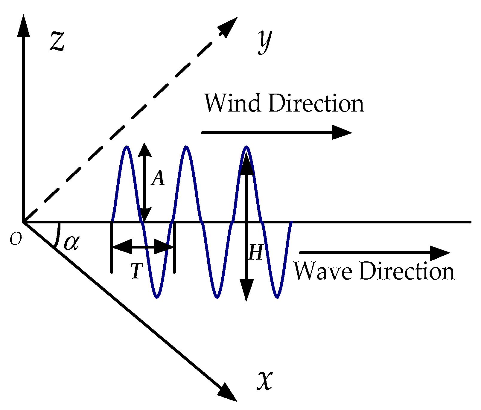
The sea surface motion is a random and time-varying process and is assumed to consist of the random waves with the various heights, lengths, and directions. The random phase or amplitude model is the basic model for describing the moving sea surface elevation [31,32]. The sea surface wave is considered to be the sum of a large number of harmonic waves, and each of these waves can be represented with a sinusoidal long-crested progressive wave, as shown in Figure 4.
As shown in Figure 4, the orbital velocity of the long waves is time-varying and space-varying, the wave profile is the linear superposition of sinusoidal waves, and the orbital velocity of the long waves possesses the periodicity shown in Figure 4 [3,33]. The orbital velocity of the long waves is modeled as the function of time t and slant range r and can be written as Xin et al. [3]:
where is the number of harmonic waves, is the amplitude of the ith harmonic sinusoidal wave, is the angular velocity of the ith sinusoidal wave and is the wavenumber of the ith wave. , and g is the acceleration due to gravity. is the random phase and is uniformly distributed. is the propagation direction of the long orbital wave. Therefore, can be written as:
The two-scale model [34] is widely used to describe the SAR imaging mechanism of ocean waves, and for sea surface imaging, the cross-section modulation consists of three components: tilt modulation, hydrodynamic modulation, and orbital motion modulation [32]. Since the three mechanisms interact, the sea surface wave is no longer described by the simple linear superposition of sinusoidal waves, as shown in Figure 5.
As illustrated above, the SAR imaging of ocean waves has an additional source of modulation due to the effect of orbital motions. This effect is often the dominant imaging mechanism for waves propagating in the azimuthal direction. The range-to-platform velocity ratio R/V is the key parameter for the sea surface waves of SAR. When R/V < 50 s, the variation of the sea surface is so small that the azimuthal offset can be neglected. In addition, at a moderate sea state or wind speed, the contribution of wave modulations is very small at moderate grazing angles and, thus, the long orbital waves can be modeled as the linear superposition of sinusoidal waves.
In this paper, our work considers the aforementioned general case. Therefore, the Doppler shift caused by the orbital velocity of the long waves can be neglected by averaging over a large area greater than the length of the long sea surface wave. After averaging over the certain spatial scales, the additional residual orbital velocity is usually small, so the orbital velocity can be approximated as zero.
3.1.4. Doppler Shift of the Platform Motion
The Doppler shift caused by the platform motion changes with the rotation of the antenna scanning beam at a fixed incidence angle [10]. For convenience, the Doppler shift for the varying azimuth angles can be written as:
3.2. Practical Model of the Doppler Centroid Shift
In the practical model of the Doppler centroid shift, after compensating for the aircraft platform motion based on the high-precision inertial measurement unit (IMU) and Global Position System (GPS), which record the antenna position parameters, there remain some errors, as follows:
- (1)
- When estimating the Doppler centroid shift by applying the clutter lock method based on the energy gravity center of the Doppler spectrum of the real data [35], there exists an estimation error of the Doppler centroid shift, and the estimated Doppler centroid shift can be represented as .
- (2)
- When compensating the platform motion according to Equation (10) for all slant range cells in the same wave beam, there will exist a compensation error which contains the compensation error of the incidence angle departing from the central slant range and the residual compensation error induced by the azimuth pointing error .
Therefore, after compensating the airborne platform motion and averaging the certain slant range cells near the central slant range within the same wave beam to eliminate the effect of the orbital velocity of the long waves, the practical mean Doppler model for each scan angle can be represented as:
where is the estimated mean Doppler centroid shift, and represents the mean operator, .
3.2.1. Compensation Error of the Incidence Angle
For all range cells in the same wave beam, the Doppler shift caused by the platform motion is compensated based on Equation (10). As a consequence, the Doppler shift includes a deviation from the incidence angle departing from the central slant range after the motion compensation.
The residual Doppler shift for the slant range greater than the central slant range can be written as:
where is the angle between the greater-than-central slant range and the central slant range. As shown in Figure 1, we can obtain:
where is the range resolution and n is the number of range resolution cells departing from the central slant range.
The residual Doppler shift for the slant range less than the central slant range can be written as:
where is the angle between the less-than-central slant range and central slant range. Meanwhile, we can obtain:
when , the compensation error caused by the incidence angle can be neglected. However, when the aforementioned condition is not satisfied, the compensation error cannot be neglected and needs to be considered.
3.2.2. Doppler Shift of Azimuth Pointing Error
In fact, as the airborne platform undergoes deviations from the ideal straight trajectory, the motion compensation is based on the high-precision IMU and GPS data and is implemented during the imaging processing stage. However, for a SAR system, the radar beam possesses a fixed azimuth pointing error. Therefore, after the motion compensation of the airborne platform, the residual Doppler shift caused by the azimuth pointing error can be calculated by:
where represents the azimuth pointing error. The aforementioned equation uses the Taylor series expansion, and can be rewritten as:
3.3. Estimation of Sea Surface Current Velocity
Above all, after compensating the airborne platform motion and the Doppler shift caused by the incidence angle, averaging the spatial scales for removing the orbital motions of the long waves, substituting Equations (5) and (17) into Equation (11), and considering the azimuth pointing error for the Doppler shift of the sea surface current velocity which uses the Taylor series expansion, the estimated Doppler centroid shift for each range cell can be rewritten as:
where the range of m is from 1 to L, and L is the number of range cells.
Therefore, the estimated mean Doppler centroid shifts of the L range cells for N different scan angles can be expressed in a matrix form and can be written as:
where:
For the estimation of the unknown vector of the Equation (19), we apply the LS method. We can obtain the LS solution of , which is expressed as:
By combining Equations (21) and (23), the azimuth pointing error, the along-track velocity component, and the cross-track velocity component can be written as:
when neglecting the azimuth pointing error of the radar system, Equations (20) and (21) can be written as:
Similarly, by the LS method, we can obtain:
| Algorithm: The sea surface current estimation. |
| Input: Radar echo data Output: Ux, Uy, Δθ. For n = 1: N Process imaging and transform the data into the range Doppler domain. for m = 1:L Compute the Doppler centroid shift of every range cell |
| after the motion compensation. end for Compute the mean Doppler shift as follows: |
| end for Calculate Ux, Uy, Δθ according to the LS method as follows: |
4. Experimental Results and Analyses
4.1. Circular Scanning SAR Data
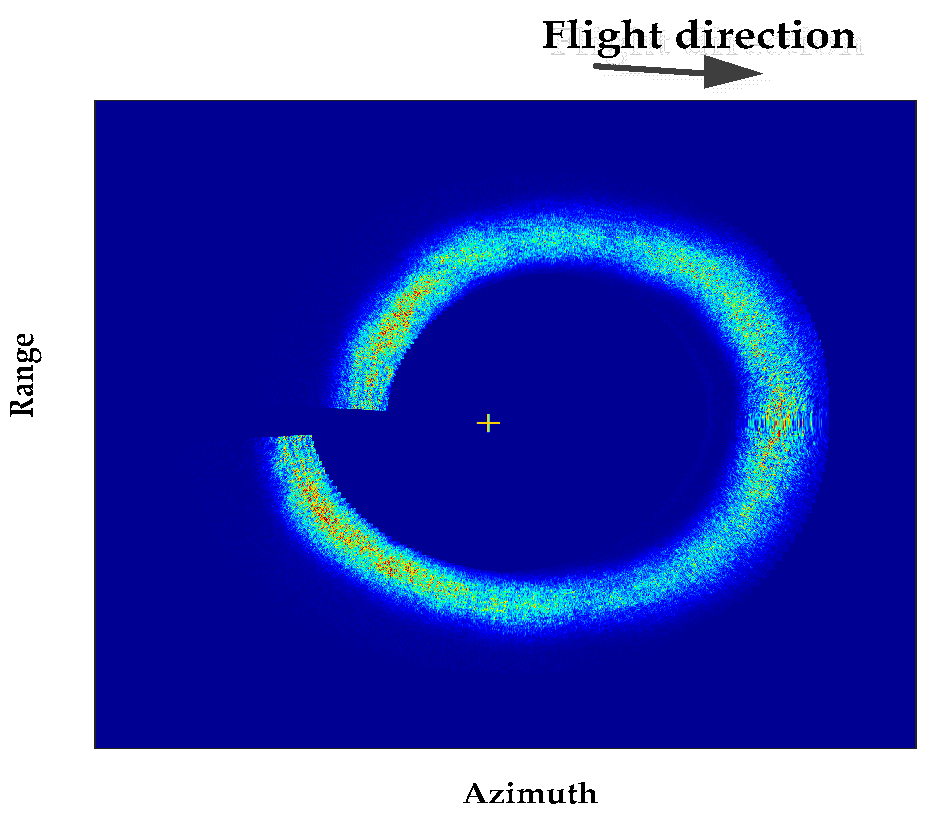
The datasets used herein were recorded by an airborne circular scanning SAR and collected on 11 January 2016 at 13:00 UTC in the Bohai Sea of China. The antenna of the system rotates at a scanning rate of 30 degrees/s around the flight direction, as introduced in Section 2, and the key parameters of the circular scanning SAR system are listed in Table 1. We selected 131 consecutive scan angles for every 2.7 degree beam scan angle. Figure 6 shows the image for the radar beams over 360 degrees and the two-dimensional swath approximates 12 km × 12 km (range × azimuth). It is clearly seen that the imaging region is close to a circle, as shown in Figure 1.
The sea surface parameters of the region of interest with 25 m water depth were measured via a marine buoy system. The measured sea surface current velocity is 0.56 m·s−1, and the velocity field is homogeneous. The key parameters of the sea surface measured by the buoy system are listed in Table 1, and the sea state is calculated by Watts [36]:
where , , and represent the wind speed, the sea state, and the significant wave height, respectively.
Figure 7a,c,e show the range Doppler images from 1.03 degree, 43.35 degree, and 89.91 degree scan angles, respectively, and Figure 7b,d,f are the normalized Doppler spectra in the central slant ranges corresponding to Figure 7a,c,e, respectively. If the sea surface is motionless, the Doppler centroid shifts should be zero for different scan angles after compensating for the airborne platform motion. However, as shown in Figure 7, it is clearly indicated that the Doppler centroid shifts are nonzero. For the range Doppler images, the motion compensation is based on the central slant range, and because the slant range cells departing from the central slant range include the compensation error, the Doppler centroid shifts are not in accordance with the central slant range as indicated in Equations (13) and (15). Only when the scan angle is 0 degrees or 180 degrees is the Doppler centroid shift consistent. Therefore, the Doppler shift induced by the incidence angle needs to be considered.
4.2. Analyses of the Sea Surface Current Velocity Estimation
In this subsection, we mainly focus on verifying the effectiveness of the proposed estimation method for the sea surface current velocity using real data from the airborne circular scanning SAR. The data are range Doppler images over scopes of 360 degrees after compensating for the platform motion. The actual sea surface current velocity is measured by the buoy during the collecting of the data of the sea surface in the same region, and the measured sea surface velocity is 0.56 m·s−1, which is used to evaluate the validity and the estimation accuracy of the proposed method for estimating the sea surface current velocity.
First, we process the imaging operation and obtain range Doppler data. We then calculate the mean Doppler centroid shifts for different scan angles, as shown in Figure 8. The estimation accuracy of the Doppler centroid shift is affected by the Doppler interval, which is calculated by the coherent processing interval (CPI). The designed PRF of the radar system is greater than the Doppler bandwidth, and the PRF satisfies the Nyquist sampling theorem. The Doppler interval is calculated by:
where M is the Doppler sampling number, . In the aforementioned equation, if M is too small, the Doppler sampling interval is quite large, resulting in a severe estimation error of the Doppler centroid shift. Therefore, when designing the system, the sampling number should not be too small to guarantee the estimation precision of the sea surface current velocity. The PRF of the data used above is 3000 Hz, and the Doppler sampling number is 2048. In this case, the Doppler sampling interval is 1.46 Hz.
To verify the effectiveness of the proposed method, Figure 9 gives the curves of the estimated line-of-sight velocities based on real data and the estimated line-of-sight velocities of the proposed method considering and neglecting the azimuth pointing error by averaging seven range resolution cells to eliminate the effect of the orbital velocity of the long waves. Note that the curve of the estimated line-of-sight velocities considering the azimuth pointing error almost coincides with the curve of the estimated line-of-sight velocities neglecting the azimuth pointing error in Figure 9. For a single azimuth angle, only the line-of-sight velocity can be estimated. However, by utilizing different scan angles, the sea surface current velocity can be extracted by the proposed method. When neglecting the azimuth pointing error, the estimated along-track velocity of the sea surface current velocity is −0.25 m·s−1, the estimated cross-track velocity is 0.78 m·s−1, and the sea surface current velocity is 0.81 m·s−1 (). When considering the azimuth pointing error, the estimated along-track velocity of the sea surface current is −0.23 m·s−1, the estimated cross-track velocity is 0.53 m·s−1, and the sea surface current velocity is 0.58 m·s−1. The estimated azimuth pointing error is 0.0036 rad. Compared with the measured sea surface current velocity of 0.56 m·s−1 from the buoy, when neglecting the azimuth pointing error, the estimation value has a considerable deviation; but when considering the effect of the azimuth pointing error, the estimated sea surface current velocity can be effectively improved and is close to the real sea surface current velocity. Therefore, the azimuth pointing error should be considered in order to acquire the highest possible estimation accuracy of the sea surface current velocity.
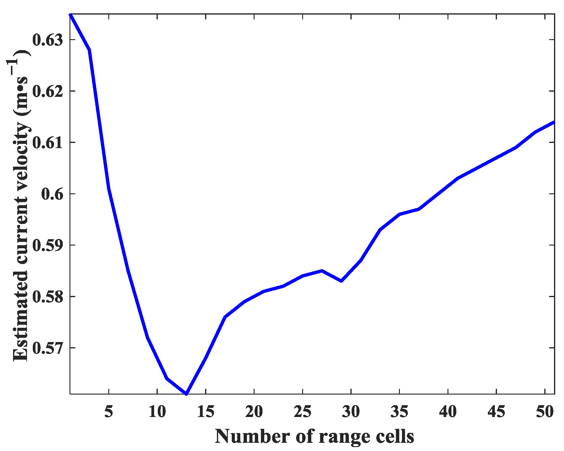
The spatial averaging processing is carried out to remove the orbital velocity of the long waves, but the choice of spatial scale will affect the estimation precision. Figure 10 shows the estimated sea surface current velocities for averaging different spatial scales, and it is clearly demonstrated that if the proposed method does not consider the spatial averaging processing, the estimated sea surface current velocity has a larger error; if averaging over an appropriate spatial scale, the estimation error can be minimized. Averaging 13 range cells, in this case, produces the minimum estimation error. Although the estimation value still contains the additional residual velocity components induced by the orbital motions of the long waves, the proposed method is practical. By the experimental analyses, we can obtain the number of range cells by choosing the minimum estimation value for averaging different range cells.
In addition, for the two-scale model, the sea backscattering coefficient is related to the radar frequency, incidence angle, wind speed, etc. Although the sea backscattering coefficient increases as the frequency increases, the three responses have the same trends [37]. For moderate wind speeds, the backscattering coefficients of the C-band, X-band, and Ku-band are similar [38]. As shown in Figure 9, at the moderate sea state, the orbital velocity of the long waves can be approximated as zero in Ku-band, which is close to that of the X-band.
Compared with the estimated sea surface velocity of the dual beam [23,24], the velocity can be written as:
As shown by the two equations above, the dual-beam technique only estimates the along-track velocity and the cross-track velocity of the sea surface. We chose the two azimuth angles in the near side-looking direction, and we can estimate the along-track velocity to be −0.97 m·s−1 and the cross-track velocity to be 0.43 m·s−1. When choosing the maximum and minimum Doppler centroid shifts to estimate the sea surface current velocity [28], the sea surface current velocity is 0.82 m·s−1, which is considerably different from the real sea surface current velocity. Therefore, according to the comparison results, the proposed method can effectively improve the estimation accuracy.
5. Conclusions
In this work, we have proposed an effective technique to estimate the sea surface current velocity in an airborne circular scanning SAR system. The effectiveness of the proposed algorithm has been verified by the processing results of real data from the airborne circular scanning SAR. Compared with the estimation method neglecting the compensation errors, because the compensation errors of the Doppler shift caused by the azimuth pointing and the incidence angle are considered, the estimation precision of the sea surface current velocity can be significantly improved. Meanwhile, compared with the conventional method, which only applies two azimuth angles, the proposed method can obtain a higher estimation precision.
Considering that the experimental analyses were performed at a moderate sea state and wind speed, the proposed approach may not always be effective for all conditions. The effect of the orbital motions of the long waves may not be averaged in the case of high sea states, strong current gradients, or internal waves. Despite these limitations, the proposed method of the sea surface current velocity estimation is valid and practical for use. How to estimate the sea surface current velocity in the case of a high sea state will be studied in our future investigations.
Acknowledgments
The authors offer significant acknowledgement to the Academy of Space Electronic Information Technology for providing the experimental sea clutter data. This work was supported, in part, by the National Natural Science Foundation of China under grants 61621005 and 61671352, the Innovational Foundation of Shanghai Academy of Space Technology under grants SAST2016027 and SAST2016033 and the Key Laboratory of Cognitive Radio and Information Processing, Ministry of Education (Guilin University of Electronic Technology) under grant CRKL160206.
Author Contributions
Guisheng Liao and Zhiwei Yang introduced this topic to Xueli Pan, and provided the technical guidance throughout the research. Xueli Pan performed the literature review and the study of the sea surface velocity estimation, and wrote the manuscript. Hongxing Dang provided the airborne circular scanning SAR data. Xueli Pan provided a full review and revision of the final manuscript.
Conflicts of Interest
The authors declare no conflict of interest.
References
- Chen, C.; Shiotani, S.; Sasa, K. Effect of ocean currents on ship navigation in the East China Sea. Ocean Eng. 2015, 104, 283–293. [Google Scholar] [CrossRef]
- Trizna, D. A model for Doppler peak spectral shift for low grazing angle sea scatter. IEEE J. Ocean. Eng. 1985, 10, 368–375. [Google Scholar] [CrossRef]
- Xin, Z.; Liao, G.; Yang, Z.; Zhang, Y.; Dang, H. A deterministic sea clutter space time model based on physical sea surface. IEEE Trans. Geosci. Remote Sens. 2016, 54, 6659–6673. [Google Scholar] [CrossRef]
- Kim, D.; Moon, W.M.; Imel, D.A.; Moller, D. Remote sensing of ocean waves and currents using NASA (JPL) AIRSAR Along-Track Interferometry (ATI). In Proceedings of the IEEE International Geoscience and Remote Sensing Symposium (IGARSS), Toronto, ON, Canada, 24–28 June 2002; pp. 931–933. [Google Scholar] [CrossRef]
- Thompson, D.R.; Graber, H.C.; Carande, R.E. Measurements of ocean currents with SAR Interferometry and HF Radar. In Proceedings of the IEEE International Geoscience and Remote Sensing Symposium (IGARSS), Pasadena, CA, USA, 8–12 August 1994; pp. 2020–2022. [Google Scholar] [CrossRef]
- Martin, R.J.; Kearney, M.J. Remote sea current sensing using HF Radar: An autoregressive approach. IEEE J. Ocean. Eng. 1997, 22, 151–155. [Google Scholar] [CrossRef]
- Zhang, J.; Walsh, J.; Gill, E.W. Inherent limitations in high-frequency radar remote sensing based on Bragg scattering from the ocean surface. IEEE J. Ocean. Eng. 2012, 37, 395–405. [Google Scholar] [CrossRef]
- Chang, G.; Li, M.; Xie, J.; Zhang, L.; Yu, C.; Ji, Y. Ocean surface current measurement using shipborne HF radar: Model and analysis. IEEE J. Ocean. Eng. 2016, 41, 970–981. [Google Scholar] [CrossRef]
- Chapron, B.; Collard, F.; Ardhuin, F. Direct measurements of ocean surface velocity from space: Interpretation and validation. J. Geophys. Res. Oceans 2005, 110, 691–706. [Google Scholar] [CrossRef]
- Braun, N.; Ziemer, F.; Bezuglov, A.; Cysewski, M.; Schymura, G. Sea surface current features observed by Doppler radar. IEEE Trans. Geosci. Remote Sens. 2008, 46, 1125–1133. [Google Scholar] [CrossRef]
- Rossi, R.; Runge, H.; Breit, H.; Fritz, T. Surface current retrieval from Terrasar-X data using Doppler measurements. In Proceedings of the IEEE 5th Asia-Pacific Conference on Synthetic Aperture Radar (APSAR), Honolulu, HI, USA, 25–30 July 2010; pp. 3055–3058. [Google Scholar] [CrossRef]
- Hansen, M.W.; Collard, F.; Dagestad, K.F.; Johannessen, J.A.; Fabry, P.; Chapron, B. Retrieval of sea surface range velocities from Envisat ASAR Doppler centroid measurements. IEEE Trans. Geosci. Remote Sens. 2011, 49, 3582–3591. [Google Scholar] [CrossRef]
- Kang, K.; Kim, D. Retrieval of sea surface velocity during tropical cyclones from RADARSAT-1 ScanSAR Doppler centroid measurement. In Proceedings of the IEEE 5th Asia-Pacific Conference on Synthetic Aperture Radar (APSAR), Singapore, 1–4 September 2015; pp. 610–613. [Google Scholar] [CrossRef]
- Trizna, D.B. Coherent marine radar measurements of ocean surface currents and directional wave spectra. In Proceedings of the 2011 IEEE Oceans, Santander, Spain, 6–9 June 2011; pp. 1–5. [Google Scholar] [CrossRef]
- Carrasco, R.; Horstmann, J.; Seemann, J. Significant wave height measured by coherent x-band radar. IEEE Trans. Geosci. Remote Sens. 2017, 55, 5355–5365. [Google Scholar] [CrossRef]
- Senet, C.; Seemann, M.J.; Flampouris, S.; Ziemer, F. Determination of bathymetric and current maps by the method DiSC based on the analysis of nautical X-band radar image sequences of the sea surface. IEEE Trans. Geosci. Remote Sens. 2007, 46, 2267–2279. [Google Scholar] [CrossRef]
- Ludeno, G.; Reale, F.; Dentale, F.; Carratelli, P.E.; Natale, A.; Soldovieri, F.; Serafino, F. An X-Band radar system for bathymetry and wave field analysis in harbor area. Sensors 2015, 15, 1691–1707. [Google Scholar] [CrossRef] [PubMed]
- Shen, C.X.; Huang, W.M.; Gill, E.W. An alternative method for surface current extraction from X-band marine radar images. In Proceedings of the IEEE International Geoscience and Remote Sensing Symposium (IGARSS), Quebec City, QC, Canada, 13–18 July 2014; pp. 4370–4373. [Google Scholar] [CrossRef]
- Romeiser, R.; Thompson, D.R. Numerical study on the along-track interferometric radar imaging mechanism of oceanic surface currents. IEEE Trans. Geosci. Remote Sens. 2000, 38, 446–458. [Google Scholar] [CrossRef]
- Suchandt, S.; Runge, H. Ocean surface observations using the TanDEM-X satellite formation. IEEE J. Sel. Top. Appl. Earth Obs. Remote Sens. 2015, 8, 5096–5105. [Google Scholar] [CrossRef]
- Kim, D.; Moon, W.M. Investigation of ocean waves and currents with PacRim along-track interferometry (ATI). In Proceedings of the IEEE International Geoscience and Remote Sensing Symposium (IGARSS), Sydney, Australia, 9–13 July 2001; pp. 1415–1417. [Google Scholar] [CrossRef]
- Romeiser, R.; Runge, H.; Suchandt, S.; Kahle, R.; Rossi, C.; Bell, P.S. Quality assessment of surface current fields from TerraSAR-X and TanDEM-X along-track interferometry and Doppler centroid analysis. IEEE Trans. Geosci. Remote Sens. 2014, 52, 2759–2772. [Google Scholar] [CrossRef]
- Toporkov, J.V.; Perkovic, D.; Farquharson, G.; Sletten, M.A.; Frasier, S.J. Sea surface velocity vector retrieval using dual-beam interferometry: First demonstration. IEEE Trans. Geosci. Remote Sens. 2005, 43, 2494–2502. [Google Scholar] [CrossRef]
- Frasier, S.J.; Camps, A.J. Dual-beam interferometry for ocean surface current vector mapping. IEEE Trans. Geosci. Remote Sens. 2001, 39, 401–414. [Google Scholar] [CrossRef]
- Kim, D.; Moon, W.M.; Moller, D.; Imel, D.A. Measurements of ocean surface waves and currents using L- and C-Band along-track interferometric SAR. IEEE Trans. Geosci. Remote Sens. 2003, 41, 2821–2832. [Google Scholar] [CrossRef]
- Bao, Q.; Dong, X.; Zhu, D.; Lang, S.; Xu, X. The feasibility of ocean surface current measurement using pencil-beam rotating scatterometer. IEEE J. Sel. Top. Appl. Earth Obs. Remote Sens. 2015, 8, 3441–3451. [Google Scholar] [CrossRef]
- An, C.; He, X.; Chen, Z. Theoretical Analysis of circular-scanning SAR based on resolution and imaging efficiency comparison. In Proceedings of the 2010 2nd International Workshop on Intelligent Systems and Applications (ISA), Wuhan, China, 22–23 May 2010; pp. 1–4. [Google Scholar] [CrossRef]
- Xin, Z.; Liao, G.; Yang, Z. Estimation of current velocity using circular SAR data. Electron. Lett. 2016, 52, 1482–1484. [Google Scholar] [CrossRef]
- Plant, W.J.; Keller, W.C. Evidence of Bragg scattering in microwave Doppler spectra of sea return. J. Geophys. Res. Oceans 1990, 95, 16299–16310. [Google Scholar] [CrossRef]
- Zapevalov, A.S. Bragg scattering of centimeter electromagnetic radiation from the sea surface: The effect of waves longer than Bragg components. Izv. Atmos. Ocean. Phys. 2009, 45, 253–261. [Google Scholar] [CrossRef]
- Holthuijsen, L.H. Waves in Ocean and Coastal Waters; Cambridge University Press: Cambridge, UK, 2007. [Google Scholar]
- Li, X. Ocean Surface Wave Measurement Using SAR Wave Mode Data. Ph.D. Thesis, University Hamburg, Hamburg, Germany, 2010. [Google Scholar]
- Rheem, C.K. Measurement of directional spectrum of sea surface waves by using a microwave pulse Doppler radar with two fixed antennas. In Proceedings of the 2011 Oceans, Waikoloa, HI, USA, 19–22 September 2011; pp. 1–6. [Google Scholar] [CrossRef]
- Durden, S.; Vesescky, J. A physical radar cross-section model for a wind driven sea with swell. IEEE J. Ocean. Eng. 1985, 10, 445–451. [Google Scholar] [CrossRef]
- Wang, Y.L.; Yan, L.; Wang, Y.K. Improved Algorithm of Doppler centroid estimation for air-borne synthetic aperture radar. Acta Geod. Cartogr. Sin. 2010, 39, 271–275. [Google Scholar]
- Watts, S.; Rosenberg, L.; Bocquet, S.; Ritchie, M. Doppler spectra of medium grazing angle sea clutter part 2: Model assessment and simulation. IET Radar Sonar Navig. 2016, 10, 32–42. [Google Scholar] [CrossRef]
- Polverari, F.; Mori, S.; Pierdicca, N.; Marzano, F.S. Precipitation signature on side-looking aperture radar imaging: Sensitivity analysis to surface effects at C, X and Ku band. In Proceedings of the European Radar Conference (EuRAD), Rome, Italy, 8–10 October 2014; pp. 197–200. [Google Scholar] [CrossRef]
- Song, D.; Shang, S.; Luo, X. The study of microwave scattering of anisotropic sea surface with the corrected two-scale model. In Proceedings of the European Radar Conference (EuRAD), Paris, France, 9–11 September 2015; pp. 545–547. [Google Scholar] [CrossRef]
Figure 1.
Schematic geometry of the airborne circular scanning SAR.
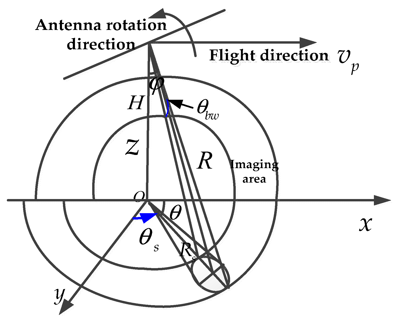
Figure 2.
Variation of the azimuth resolution with the scan angle.
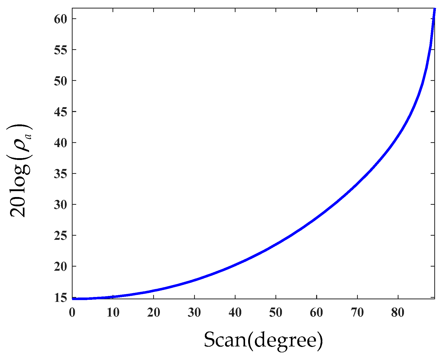
Figure 3.
Schematic diagram of the decomposition of the sea surface current velocity.
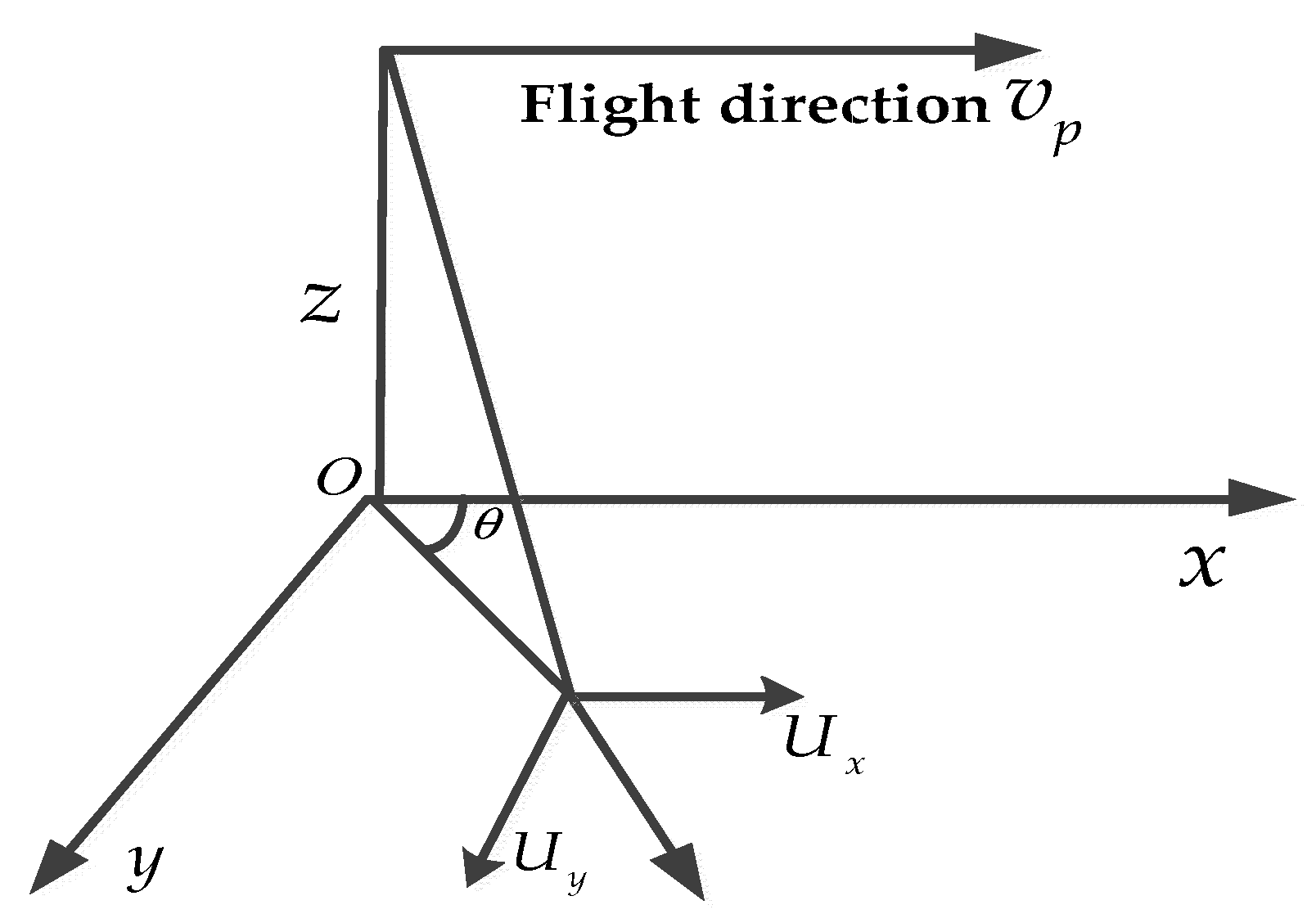
Figure 4.
Schematic diagram of a long wave.

Figure 5.
Scattering mechanism of the two-scale model.
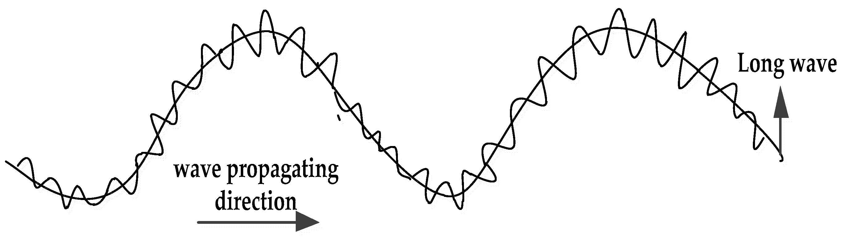
Figure 6.
SAR image of the antenna rotating a circuit.

Figure 7.
Range Doppler images and normalized Doppler spectra in different scan angles: (a) Original image at the 1.03 degree scan angle; (b) normalized Doppler spectrum for (a) in the central slant range; (c) original image at the 43.35 degree scan angle; (d) normalized Doppler spectrum for (c) in the central slant range; (e) original image at the 89.91 degree scan angle; and (f) normalized Doppler spectrum for (e) in the central slant range.
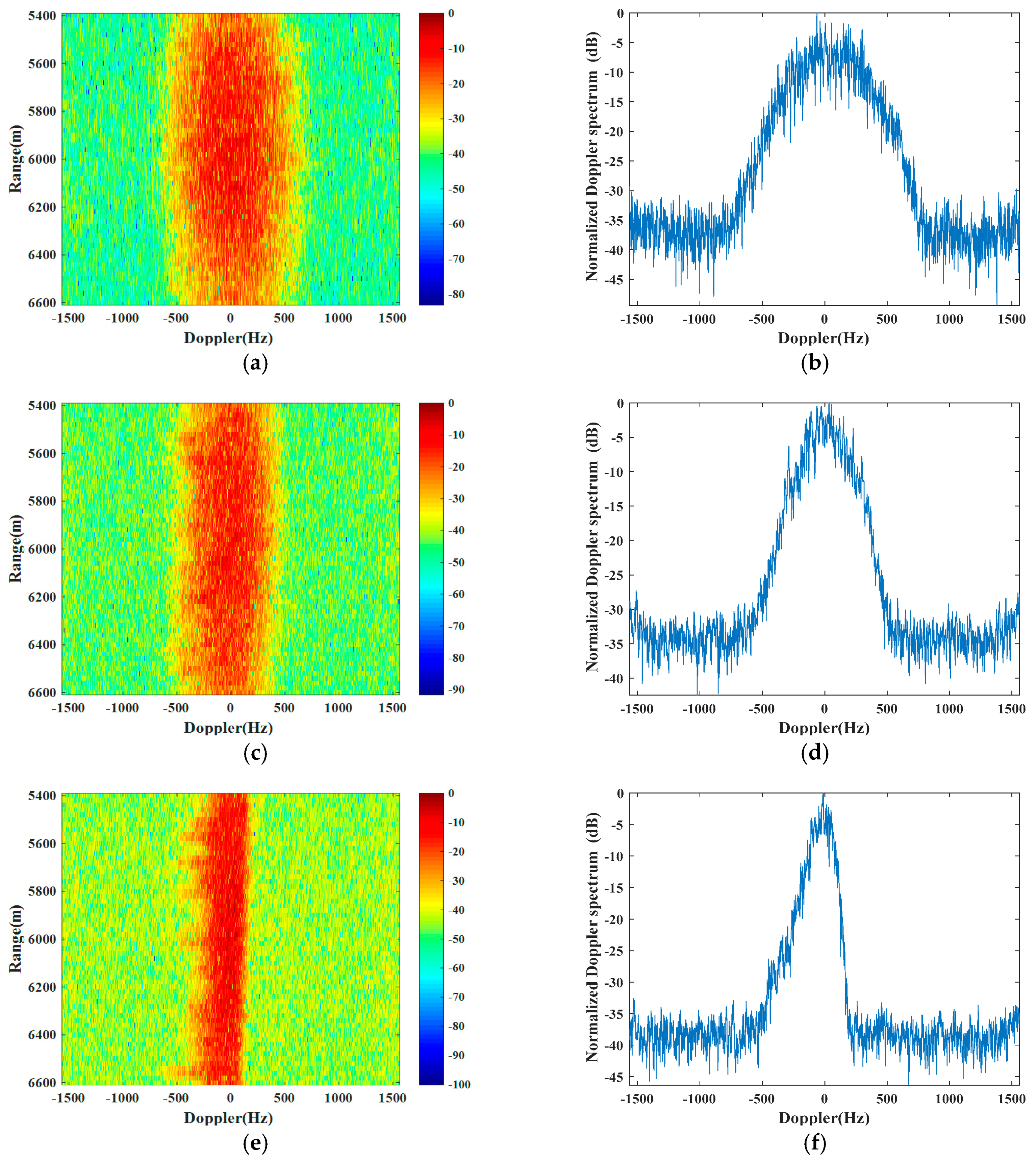
Figure 8.
Estimated Doppler centroid shifts.
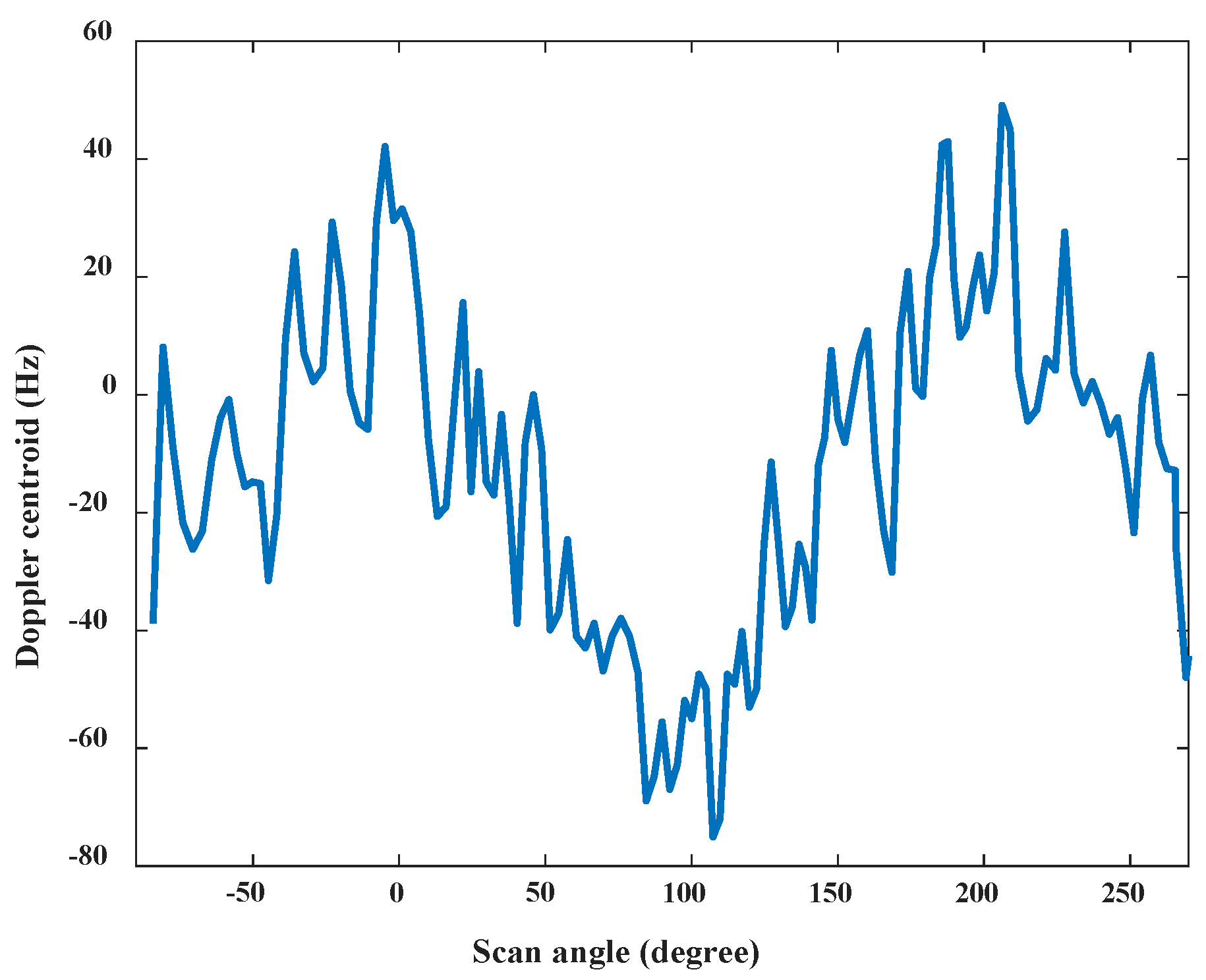
Figure 9.
Curves of estimated line-of-sight velocities.
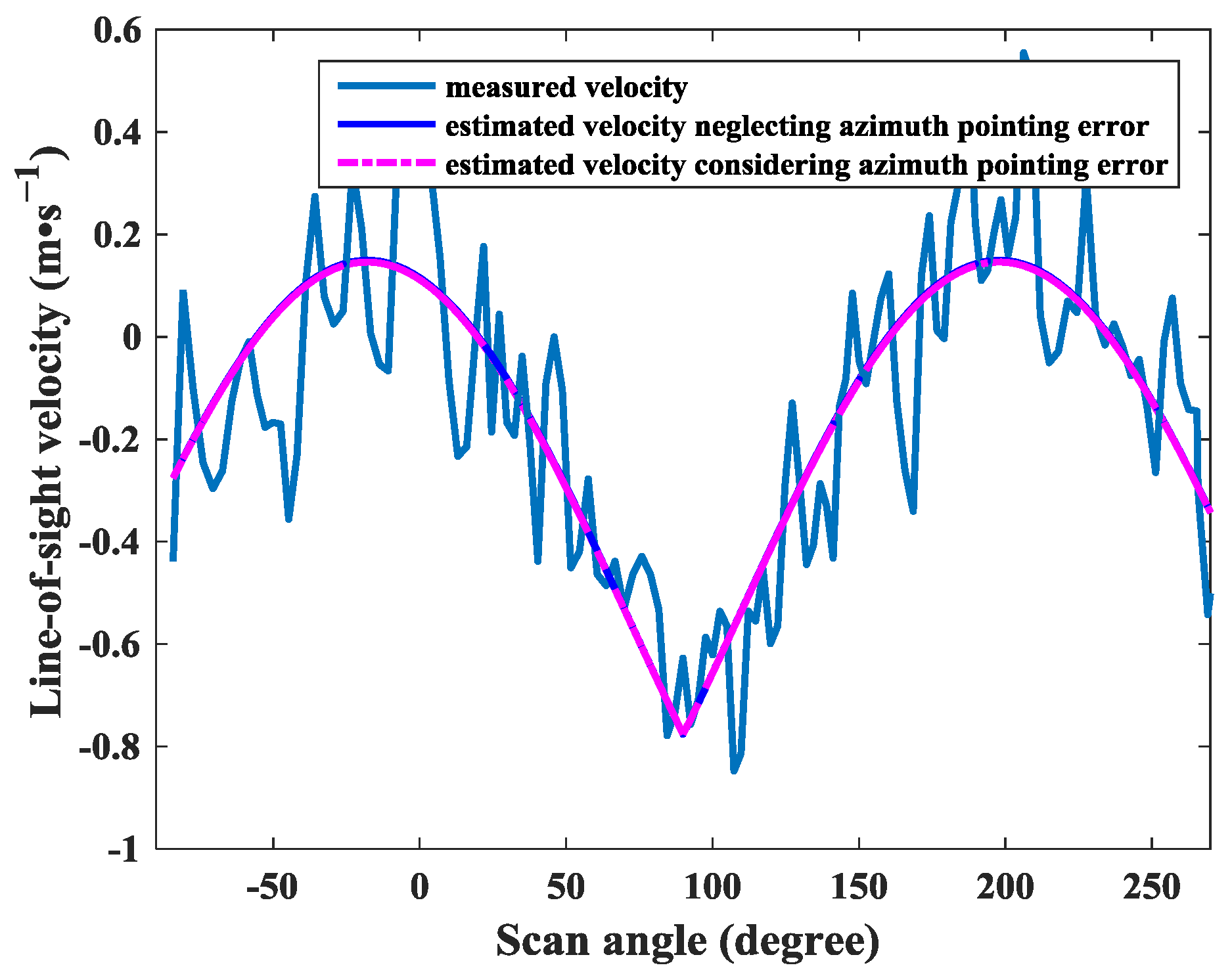
Figure 10.
Curve of the estimated sea surface current velocities for averaging different spatial scales.
Figure 10.
Curve of the estimated sea surface current velocities for averaging different spatial scales.


Table 1.
Key parameters of the circular scanning SAR and sea surface.
| Parameters | Values |
|---|---|
| Antenna beam width(azimuth/pitch) | 6.2/6.4 degree |
| Rader frequency | 13 GHz |
| Range resolution | 20 m |
| Platform speed | 130 m·s−1 |
| Platform flight height | 3000 m |
| Antenna scanning rate | 30 degrees·s−1 |
| Pulse repetition frequency (PRF) | 3000 Hz |
| Grazing angle of beam center | 35 degree |
| Wind speed | 7.8 m·s−1 |
| Sea state | 3 level |
| Significant wave height | 2.0 m |
| Polarization | HH |
© 2018 by the authors. Licensee MDPI, Basel, Switzerland. This article is an open access article distributed under the terms and conditions of the Creative Commons Attribution (CC BY) license (http://creativecommons.org/licenses/by/4.0/).
Share and Cite
MDPI and ACS Style
Pan, X.; Liao, G.; Yang, Z.; Dang, H. Sea Surface Current Estimation Using Airborne Circular Scanning SAR with a Medium Grazing Angle. Remote Sens. 2018, 10, 178. https://doi.org/10.3390/rs10020178
AMA Style
Pan X, Liao G, Yang Z, Dang H. Sea Surface Current Estimation Using Airborne Circular Scanning SAR with a Medium Grazing Angle. Remote Sensing. 2018; 10(2):178. https://doi.org/10.3390/rs10020178
Chicago/Turabian StylePan, Xueli, Guisheng Liao, Zhiwei Yang, and Hongxing Dang. 2018. "Sea Surface Current Estimation Using Airborne Circular Scanning SAR with a Medium Grazing Angle" Remote Sensing 10, no. 2: 178. https://doi.org/10.3390/rs10020178
Note that from the first issue of 2016, this journal uses article numbers instead of page numbers. See further details here.